1 Motivation

Survey data are foundational to empirical research in political science, yet rising nonresponse and selection bias threaten the validity of the inferences drawn from them (Cavari and Freedman Reference Cavari and Freedman2023; Jackman and Spahn Reference Jackman and Spahn2019; Meng Reference Meng2018). Widely used adjustments such as post-stratification or raking can align respondents with population margins on observed demographics, but they can remain biased when respondents differ systematically from nonrespondents on the outcome itself (Bailey Reference Bailey2024, Reference Bailey2025).

The core problem is nonignorable nonresponse: the likelihood of responding depends on the unobserved outcome itself. While several frameworks address this issue,Footnote ¹ the variable-response-propensity (VRP) estimator proposed by Peress (Reference Peress2010) remains distinctive. Building on “continuum of resistance” logic, VRP leverages a response-propensity proxy observed among respondents (e.g., interviewer-coded cooperativeness, a respondent’s rating of the interview or related paradata) to extrapolate from low-propensity respondents toward nonrespondents, while directly integrating observable covariates into the correction framework and retaining the benefits of post-stratification with known population shares.

However, the original VRP estimator is framed for binary outcomes, while many key survey measures in political science, such as trust, satisfaction and economic evaluations, rely on ordinal scales. Collapsing ordinal outcomes to binary discards information and can change substantive conclusions, especially if selection operates differently across the response scale (Lauderdale, Hanretty, and Vivyan Reference Lauderdale, Hanretty and Vivyan2018; Stromberg Reference Stromberg1996).

This letter provides a practical method for correcting nonignorable nonresponse in ordinal survey data when a response-propensity proxy is available, generalizing VRP beyond binary outcomes. The estimator is computed via maximum likelihood and implemented in a compact R routine covering both ordinal and binary outcomes, extending the original binary-only C++ implementation of Peress (Reference Peress2010). Our method complements recent experimental approaches to nonignorable nonresponse correction (Bailey Reference Bailey2025), as it can be applied to observational surveys without requiring randomized instruments. It further complements the semiparametric approach of Li et al. (Reference Li, Ying, Li, Shi and Miao2026), which leverages callback data (outcome variation across successive survey contact stages) to achieve identification without distributional assumptions for binary outcomes, while our method can be applied to ordinal outcomes in surveys without a multi-stage callback design.

An illustration of our approach using the 2024 American National Election Study (ANES) shows that accounting for nonignorable nonresponse can produce meaningful shifts for some outcomes (e.g., life satisfaction) but small or negligible changes for others (e.g., views on the death penalty), underscoring that the value of nonresponse correction is outcome-specific and empirically testable.

2 Problem formulation

We now generalize the VRP framework (Peress Reference Peress2010) for ordinal outcomes. Let $y_n \in \{1,2,\dots ,Y\}$ denote an ordinal outcome of interest for unit n and let $r_n$ denote an ordinal response-propensity proxy recorded among respondents, taking values in $\{1,2,\dots ,R\}$ and ordered so that smaller values indicate higher propensity to respond. We embed unit nonresponse as an additional category $R{+}1$ in the response equation: $r_n=R{+}1$ corresponds to unit nonresponse, in which case $y_n$ is missing. The key parameter is $\rho $ , the correlation between latent errors in the outcome and response equations, which captures nonignorable selection on the (unobserved) outcome after conditioning on covariates.

Operationally, we observe $(y_n,r_n,x_n,z_n)$ 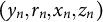only for respondents ( $r_n\le R$ ). Unit nonresponse enters through the number of missing units $N_{\text {miss}}$ (known when the sampling-frame response rate is available, or treated as a sensitivity parameter in public releases) and through population shares of strata defined by z: we partition the population into K strata indexed by k with covariate profile $z_k$ and population share $p_k^{z}$ (with $\sum _{k=1}^K p_k^{z}=1$ ).

We model the joint outcome and response processes using correlated latent-variable ordered probit models:

(1) $$ \begin{align} \begin{array}{c@{\hskip 1cm}c} \textit{Outcome model} & \textit{Response model} \\[0.8em] \begin{array}{l} y_n \in \{1,2,3,\ldots,Y\} \\[0.5em] y_n^* = \alpha^T x_n + \epsilon_n \\[0.5em] y_n = \begin{cases} 1 & \text{if } y_n^* \le \lambda_1 \\ 2 & \text{if } y_n^* \in (\lambda_1,\lambda_2] \\ 3 & \text{if } y_n^* \in (\lambda_2,\lambda_3] \\ \vdots \\ Y & \text{if } y_n^*> \lambda_{Y-1} \end{cases} \end{array} & \begin{array}{l} r_n \in \{1,2,3,\ldots,R, R+1\} \\[0.5em] r_n^* = \beta^T z_n + \eta_n \\[0.5em] r_n = \begin{cases} 1 & \text{if } r_n^* \le \theta_1 \\ 2 & \text{if } r_n^* \in (\theta_1,\theta_2] \\ 3 & \text{if } r_n^* \in (\theta_2,\theta_3] \\ \vdots \\ R & \text{if } r_n^* \in (\theta_{R-1},\theta_R] \\ R+1 & \text{if } r_n^* > \theta_R \end{cases} \end{array} \\[2em] { \displaystyle \text{corr}(\epsilon_n,\eta_n) = \rho. } \end{array} \end{align} $$

Errors $(\epsilon _n,\eta _n)$ are assumed to be jointly normally distributed with unit variancesFootnote ² and parameters $(\alpha , \beta , \lambda , \theta ,\rho )$ of model (1) are estimated via maximum likelihood, while parameters $\lambda _{Y-1}$ and $\theta _R$ are normalized to be equal to zero. The log-likelihood function takes the following form:

$$\begin{align*}\begin{aligned} \log L(\alpha,\beta,\lambda,\theta,\rho \mid y_n,r_n,x_n,z_n) &= \sum_{n=1}^N \sum_{r=1}^R \sum_{y=1}^Y \mathbf{1}\{r_n = r,\, y_n = y\} \\ &\quad \times \log \int \mathbf{1}\{\lambda_{y-1} \leq \alpha^T x_n + \epsilon \leq \lambda_{y},\, \theta_{r-1} \leq \beta^T z_n + \eta \leq \theta_{r}\} \\ &\quad \times \phi(\epsilon,\eta)\, d\epsilon\, d\eta \\[0.5em] &\quad + N_{\text{miss}} \cdot \log \sum_{k=1}^K p_k^z \int \mathbf{1}\{\beta^T z_k + \eta \geq \theta_R\}\, \phi(\eta)\, d\eta. \end{aligned} \end{align*}$$

Standard errors are derived using the delta method with numerical Jacobian matrix. This method essentially uses a parametric model to extrapolate from low-probability responders into nonresponders. While relying on a parametric model may seem restrictive, as Peress (Reference Peress2010) noted, some amount of extrapolation is necessary regardless of its technical form. Simulations in Peress (Reference Peress2010) documented meaningful gains in the case of a binary outcome. In Appendix C of the Supplementary Material, we show that the proposed estimator improves over a naïve ordinal probit model (which assumes MAR) and over the binarized version of the binary VRP approach of Peress (Reference Peress2010) across a range of scenarios.

3 Empirical illustration

We illustrate the proposed method using the Preliminary Release of the 2024 ANES (dated February 19, 2025) (American National Election Studies 2025). The dataset contains approximately 3,000 respondents. The 2024 ANES Time Series Study reports AAPOR RR1 response rates of 33.4% (in-person) and 37.7% (web) (American National Election Studies 2025), corresponding to nonresponse rates of roughly 67% and 62%. We therefore use 65% nonresponse rate for the headline results.

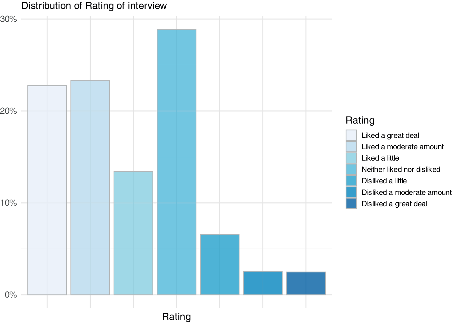
As a response-propensity proxy, we use the respondent’s own rating of the interview with seven levels and Figure 1 captures its distribution. Other potential candidates for response variables such as rating of the interviewer or do you take survey seriously were not used due to their limited variability (see Appendix A of the Supplementary Material). The covariates consist of marital status, spouse’s gender (three categories: male, female or inapplicable), race and education (five levels), which together define 60 strata.

Figure 1.

Distribution of the response variable Rating of interview.

Figure 1. Long description

The vertical y-axis represents percentage from 0 percent to 30 percent in increments of 10. The horizontal x-axis is labeled Rating and contains seven vertical bars. From left to right, the bars represent a gradient from light blue to dark blue.

* The first bar, Liked a great deal, reaches approximately 23 percent.

* The second bar, Liked a moderate amount, reaches approximately 24 percent.

* The third bar, Liked a little, reaches approximately 14 percent.

* The fourth bar, Neither liked nor disliked, is the highest peak at approximately 29 percent.

* The fifth bar, Disliked a little, drops significantly to approximately 6 percent.

* The sixth bar, Disliked a moderate amount, is approximately 3 percent.

* The seventh bar, Disliked a great deal, is approximately 3 percent.

A legend on the right side maps the color gradient to the specific rating labels in the same order as the x-axis.

Following Peress (Reference Peress2010), we set $z_n=x_n$ in the main specification. This preserves the comparison with the original binary VRP estimator and avoids restricting the analysis to subsamples defined by mode-specific paradata; Appendix D of the Supplementary Material reports a robustness check that adds a candidate exclusion-restriction variable to $z_n$ and shows the conclusions are unchanged.

We use the respondent’s self-reported rating of the interview as the VRP proxy for response propensity. In the same spirit, Peress (Reference Peress2010) uses an interviewer-coded measure of cooperativeness for this role; a respondent’s own rating of the interview plays the same part, ordering respondents by willingness to cooperate and providing leverage for extrapolating from low-propensity respondents toward nonrespondents. In our application, the proxy displays substantial dispersion (Figure 1), and we assess the implied monotonic relationship by examining outcome distributions across proxy categories (upper panels of Figures 2 and 3).

Figure 2.

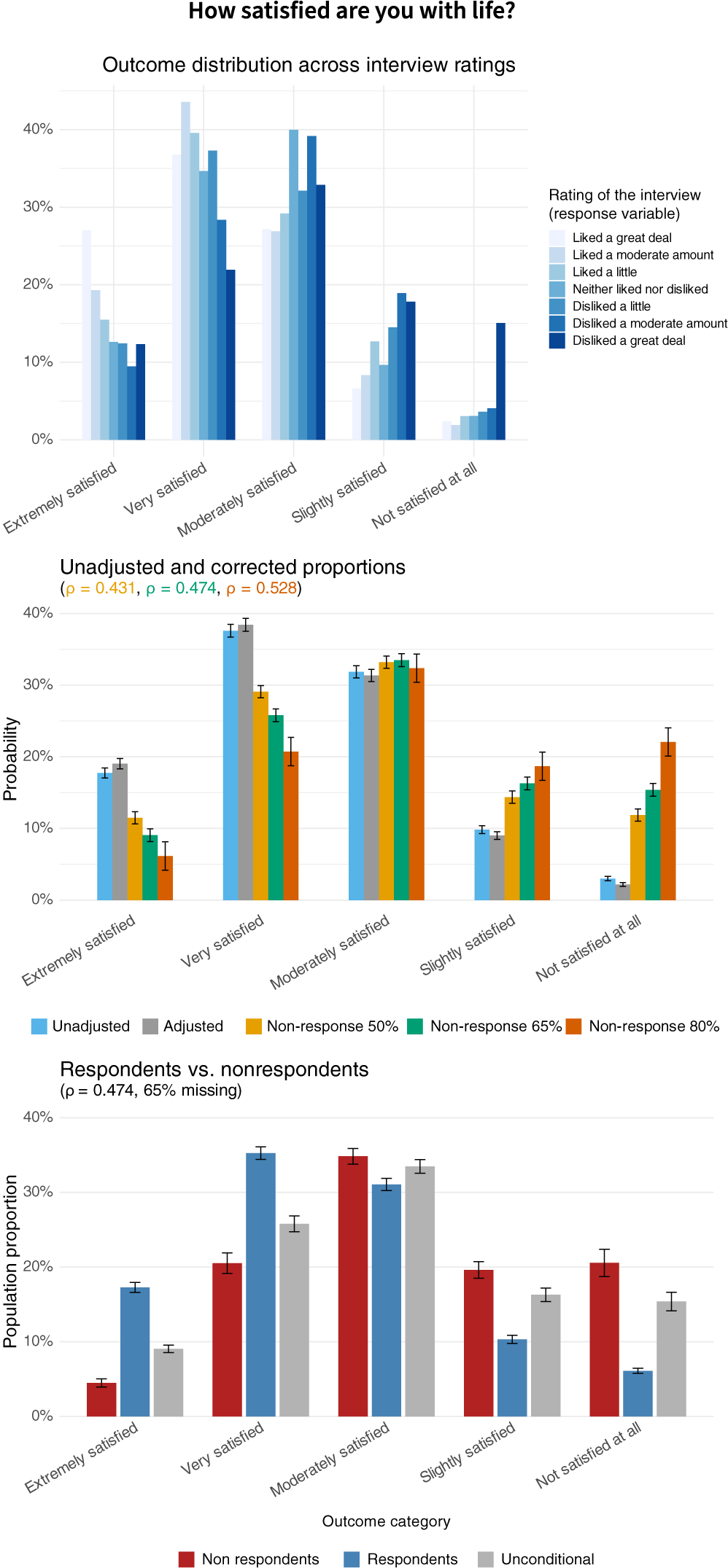
Question How satisfied are you with life? The upper panel shows the distribution of the response to this question across different ratings of the interview. The middle panel shows the unadjusted raw proportions, survey-weighted proportions and proportions estimated with the method proposed in this letter for different nonresponse rates: 50%, 65% and 80%. The lower panel shows the comparison of the estimated distributions for the overall population, nonrespondents and respondents with 65% nonresponse rate.

Figure 2. Long description

The multi-panel bar chart is organized vertically into three sections.

Top Panel: Outcome distribution across interview ratings. The Y axis shows percentages from 0% to 40%. The X axis lists five categories: Extremely satisfied, Very satisfied, Moderately satisfied, Slightly satisfied, and Not satisfied at all. Each category contains seven bars representing interview ratings from ‘Liked a great deal’ (lightest blue) to ‘Disliked a great deal’ (darkest blue). A clear trend shows that those who liked the interview more report higher life satisfaction, while those who disliked it report lower satisfaction.

Middle Panel: Unadjusted and corrected proportions. The Y axis measures Probability from 0% to 40%. It compares five data series: Unadjusted (light blue), Adjusted (grey), and three nonresponse scenarios: 50% (yellow), 65% (green), and 80% (orange). As nonresponse rates increase, the probability of ‘Extremely satisfied’ and ‘Very satisfied’ decreases, while ‘Slightly satisfied’ and ‘Not satisfied at all’ increase.

Bottom Panel: Respondents versus nonrespondents at a 65% missing rate. The Y axis shows Population proportion from 0% to 40%. It compares three groups: Non respondents (red), Respondents (blue), and Unconditional (grey). Nonrespondents show significantly higher proportions in the ‘Not satisfied at all’ and ‘Slightly satisfied’ categories compared to respondents, who are more concentrated in the ‘Very satisfied’ and ‘Moderately satisfied’ categories.

Figure 3.

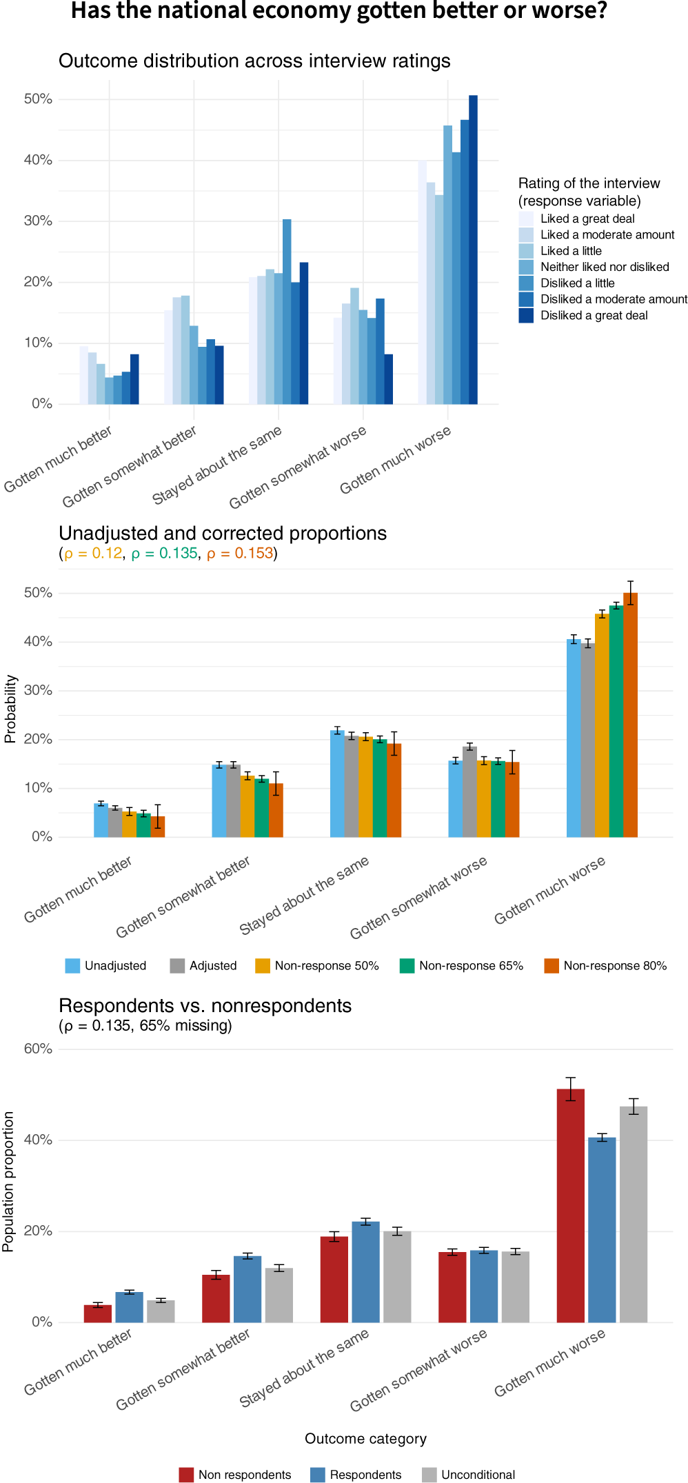
Question Has national economy gotten better or worse? The upper panel shows the distribution of the response to this question across different ratings of the interview. The middle panel shows the unadjusted raw proportions, survey-weighted proportions and proportions estimated with the method proposed in this letter for different nonresponse rates: 50%, 65% and 80%. The lower panel shows the comparison of the estimated distributions for the overall population, nonrespondents and respondents with a 65% nonresponse rate.

Figure 3. Long description

The figure consists of three vertically stacked bar charts sharing a common X axis of five categories: Gotten much better, Gotten somewhat better, Stayed about the same, Gotten somewhat worse, and Gotten much worse.

* Top Panel: Outcome distribution across interview ratings. The Y axis shows percentage from 0 to 50. Seven bars per category represent interview ratings from Liked a great deal (lightest blue) to Disliked a great deal (darkest blue). The Gotten much worse category shows a clear trend where those who disliked the interview were more likely to report the economy got much worse, peaking at over 50 percent.

* Middle Panel: Unadjusted and corrected proportions. The Y axis shows probability from 0 to 50 percent. Five bars per category compare Unadjusted (light blue), Adjusted (gray), and three nonresponse rates: 50 percent (yellow), 65 percent (green), and 80 percent (orange). Error bars are present. As the nonresponse rate increases, the probability for Gotten much worse increases from approximately 40 percent to 50 percent.

* Bottom Panel: Respondents versus nonrespondents at a 65 percent missing rate. The Y axis shows population proportion from 0 to 60 percent. Three bars per category compare Non respondents (red), Respondents (blue), and Unconditional (gray). In the Gotten much worse category, nonrespondents show a significantly higher proportion (over 50 percent) compared to respondents (approximately 40 percent).

Here, we present two different survey questions from ANES, the relationship between the outcome and response measures and then the distribution of the responses with varying degree of nonresponse together with estimated correlation coefficients.

• • Question 1: “How satisfied are you with life?”

• • Question 2: “Has national economy gotten better or worse?”

In the first question, we observe that respondents not satisfied with their life disliked the interview more (upper panel of Figure 2). This is reflected in the fact that estimates with high nonresponse assign a much larger proportion to the Slightly satisfied or Not satisfied at all categories with estimated correlation coefficients around $0.47$ . We see a mirror image on the other side of the distribution of life satisfaction. Also, we note that the proportion of respondents in the Moderately satisfied is barely affected. The model also allows us to estimate the outcome distribution separately for respondents and nonrespondents by conditioning on the latent response propensity (see Appendix B of the Supplementary Material). We observe a large difference between the nonrespondents and respondents. In this scenario, adjustment plays an important role. The life-satisfaction correction illustrates a pattern flagged by prior work on nonresponse in subjective well-being surveys: Heffetz and Rabin (Reference Heffetz and Rabin2013) show that conclusions drawn from well-being data are sensitive to the difficulty of reaching respondents, and Hudomiet, Hurd, and Rohwedder (Reference Hudomiet, Hurd and Rohwedder2021) document that differential nonresponse biases the age profile of life satisfaction upward in the Health and Retirement Study. We present this result as an illustration of sensitivity to nonignorable nonresponse rather than a definitive reassessment, and further investigation is warranted.

Figure 3 shows the results for the question on perception of the national economy. Despite variability in the response–outcome relationship (upper panel), the nonresponse-adjusted proportions shift only modestly toward the gotten worse end, with an estimated correlation around $0.14$ . The adjustment is far smaller than for life satisfaction, illustrating that the magnitude of the correction is outcome-specific.

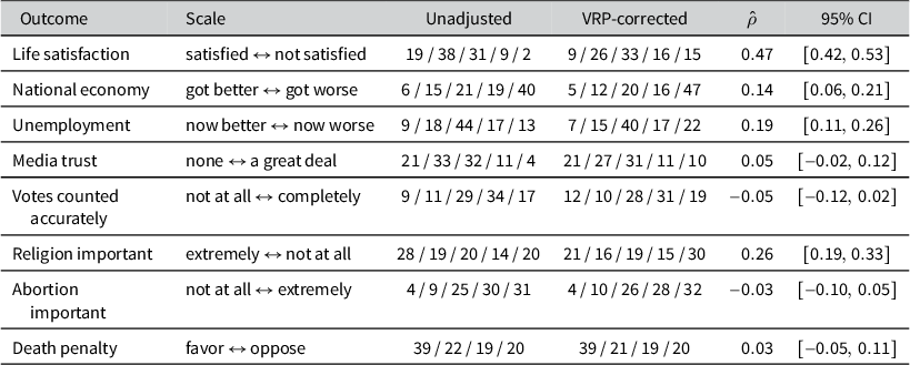
Table 1 summarizes the adjustment across all eight outcomes, adding questions on unemployment, media, elections, religion, abortion and the death penalty to the two discussed above; these are illustrated graphically in Appendix A of the Supplementary Material. The estimated selection correlation $\widehat \rho $ ranges from essentially zero to about $0.5$ . It is largest for life satisfaction ( $0.47$ ) and the importance of religion ( $0.26$ ): for these outcomes, the corrected distribution shifts toward less satisfaction with life and lower religious importance, reflecting that more reluctant respondents, and by extrapolation nonrespondents, differ systematically from eager respondents. The adjustment is moderate for unemployment ( $0.19$ ) and the national economy ( $0.14$ ), and statistically indistinguishable from zero for media trust, vote-count accuracy, abortion importance and the death penalty, where the corrected and survey-weighted distributions nearly coincide. The sign of $\widehat \rho $ records the direction of selection: a positive value indicates that respondents who were more reluctant tend toward higher outcome categories. These patterns mirror the outcome-by-proxy relationships in Appendix A of the Supplementary Material and make clear that the value of correcting for nonignorable nonresponse is outcome-specific: substantial for a few attitudinal measures and negligible for most.

Table 1

Summary of survey-weighted unadjusted and VRP-corrected population shares (percentage points, rounded) for all eight outcomes, assuming 65% nonresponse

Table 1 Long description

The table contains six columns and eight rows of data.

* Life satisfaction (satisfied to not satisfied): Unadjusted 19 / 38 / 31 / 9 / 2; V R P-corrected 9 / 26 / 33 / 16 / 15; rho-hat 0.47; 95% C I [0.42, 0.53].

* National economy (got better to got worse): Unadjusted 6 / 15 / 21 / 19 / 40; V R P-corrected 5 / 12 / 20 / 16 / 47; rho-hat 0.14; 95% C I [0.06, 0.21].

* Unemployment (now better to now worse): Unadjusted 9 / 18 / 44 / 17 / 13; V R P-corrected 7 / 15 / 40 / 17 / 22; rho-hat 0.19; 95% C I [0.11, 0.26].

* Media trust (none to a great deal): Unadjusted 21 / 33 / 32 / 11 / 4; V R P-corrected 21 / 27 / 31 / 11 / 10; rho-hat 0.05; 95% C I [minus 0.02, 0.12].

* Votes counted accurately (not at all to completely): Unadjusted 9 / 11 / 29 / 34 / 17; V R P-corrected 12 / 10 / 28 / 31 / 19; rho-hat minus 0.05; 95% C I [minus 0.12, 0.02].

* Religion important (extremely to not at all): Unadjusted 28 / 19 / 20 / 14 / 20; V R P-corrected 21 / 16 / 19 / 15 / 30; rho-hat 0.26; 95% C I [0.19, 0.33].

* Abortion important (not at all to extremely): Unadjusted 4 / 9 / 25 / 30 / 31; V R P-corrected 4 / 10 / 26 / 28 / 32; rho-hat minus 0.03; 95% C I [minus 0.10, 0.05].

* Death penalty (favor to oppose): Unadjusted 39 / 22 / 19 / 20; V R P-corrected 39 / 21 / 19 / 20; rho-hat 0.03; 95% C I [minus 0.05, 0.11].

Note: $\hat \rho $ estimates the latent selection correlation; 95% confidence intervals in brackets.