1. Introduction
In a large variety of experimental scientific domains where measurements are performed, a major challenge has to be faced: no matter the type of data acquisition, the measured quantities are only a very sparse representation of the real, and therefore inaccessible, field. This sparsity can manifest itself in several forms depending on the specific circumstances. For example, in fluid mechanics, measurements are often under-resolved in time or space, or only contain partial information about the total state. The measured field can be thought of as a low-order representation of the real field. Moreover, the measured fields are commonly contaminated by noise and thus deviate from the true values. Techniques that aim at a full reconstruction of the state vector from available (limited) data are referred to as inverse methods. The data-assimilation approach took its roots in the domain of weather forecasting where predicting the future evolution of both atmospheric and oceanic flows is based on the space–time extrapolation of unequally distributed data of different types measured at weather stations all around the world.
Several types of estimation problems can be distinguished. For example, the full state (for instance, pressure, velocity, temperature, etc.) can be estimated at a fixed time everywhere in space, or the future state-vector trajectory can also be predicted. Mathematically, both of these cases fall into the same category of inverse problems, where full information is retrieved from low-order, limited measurements. Many different methods have been developed to achieve accurate data reconstruction, ranging from simple interpolation techniques to more sophisticated approaches which take advantage of the underlying governing equations of the system. The formulation of such a problem using a variational formulation has been thoroughly studied in the meteorological community (Le Dimet & Talagrand Reference Le Dimet and Talagrand1986; Courtier Reference Courtier1997; Mohammadi & Pironneau Reference Mohammadi and Pironneau2004). A review of various data-assimilation techniques used in meteorology is given in Ghil & Malanotte-Rizzoli (Reference Ghil and Malanotte-Rizzoli1991). Recently, the interest in data-assimilation has reached fluid experimentalists, who wish to extract a maximum amount of information from their measurements. This method can therefore be applied to improve the quality of a particle image velocimetry (PIV) or magnetic resonance imaging (MRI) acquisition. This includes spatial refinement, extension of the measured fields beyond their domain of acquisition, and the reconstruction of unmeasured flow field quantities from measured ones. In this context, it is worth mentioning the ‘gappy POD’ method proposed by Everson & Sirovich (Reference Everson and Sirovich1995), based on incomplete proper orthogonal decomposition, which has been used successfully to reconstruct missing PIV snapshots (see Gunes, Sirisup & Karniadakis Reference Gunes, Sirisup and Karniadakis2006).
This paper focuses on data-assimilation using variational methods and the enforcement of the governing equations with Lagrange multipliers (or adjoint variables). This approach is widely used in the flow optimization community for finding optimal perturbations, forcings or control strategies, to cite but a few applications (Hill Reference Hill1995; Gunzburger Reference Gunzburger2000; Luchini & Bottaro Reference Luchini and Bottaro2001; Schmid Reference Schmid2007; Sipp et al. Reference Sipp, Marquet, Meliga and Barbagallo2010). The adjoint variables can be interpreted as sensitivities and therefore yield valuable information on the impact of any kind of changes in the constraints that apply to the system. A variable then has to be chosen as a design parameter (or control parameter) which will be optimized in order to identify an extremum of a cost functional measuring the deviation from the simulated state vector to the dataset of measurements. The control parameters can be of various kinds, e.g. an initial condition (Lundvall, Kozlov & Weinerfelt Reference Lundvall, Kozlov and Weinerfelt2006), a physical parameter, or a material characteristic (Avril et al. Reference Avril, Bonnet, Bretelle, Grédiac, Hild, Ienny, Latourte, Lemosse, Pagano, Pagnacco and Pierron2008). The outcome of such data-assimilation techniques is twofold: both the state and the design parameter are identified optimally, as the error between the model-based solution and the true measurements reaches a minimum. Beyond reconstructing the state vector, the application of such a methodology leads to an improvement of the model through the identification of the optimal control variable.
Variational techniques for fluid flow estimation from image sequences have been introduced recently to consistently combine image measurements with constraints expressing that the fluid behaves as a continuum material (Heitz, Mémin & Schnorr Reference Heitz, Mémin and Schnorr2010). The objective is to add physical constraints to the measurements (here snapshots of optical intensity) to improve the quality of the flow reconstruction in terms of velocity components. Classical PIV algorithms rely on correlation techniques to extract the velocity fields. More physical constraints have already been considered: optical flow model (Ruhnau et al. Reference Ruhnau, Kohlberger, Nobach and Schnorr2005), Stokes equations (Ruhnau & Schnorr Reference Ruhnau and Schnorr2007) and even time-dependent vorticity transport equations (Ruhnau, Stahl & Schnorr Reference Ruhnau, Stahl and Schnorr2007).
In the present paper, contrary to these authors, we directly consider snapshots with velocity components (for example, obtained with a PIV technique). Also, we do not aim at reconstructing a series of flow snapshots obtained at successive times but rather the time-average of these snapshots, the mean flow, and their second-order statistics, the Reynolds stresses. For this, we will use as a regularization the full Reynolds-averaged Navier–Stokes (RANS) equations. It is important to note that this choice of regularization operator (or kernel) is not unique. However, we choose the RANS equations as we believe they describe the physics of the problem accurately. The computational cost should therefore remain reasonable, even in three-dimensional configurations, since only steady-state solutions of the RANS equations and adjoint solutions, which do not involve time, need to be evaluated numerically. The approach employed in this paper can be applied to any unsteady (not necessarily turbulent) flow. Such a flow can, in a first instance, be described by its first statistical moment, the mean flow. Even if the original flow can only be fully understood using both the mean and the unsteady components, we can gain some information about the flow by replacing the full unsteady terms by the second-order momentum, i.e. the Reynolds stress tensor. The goal of the present study is to investigate the possibilities of state-vector reconstruction from sparse mean flow measurements. We presume that the mean (or time-averaged) flow satisfies the RANS equations. In this set of equations, the Reynolds stress tensor appears as an additional unknown, and its definition in terms of the mean quantities is known as the closure problem. However, in our case, this unknown is chosen as a design variable (sometimes referred to as the control parameter) in an optimization process and will be considered as an unknown forcing term in the standard, steady Navier–Stokes equations. We thus identify the full mean flow from sparse data measurements (taken from a direct numerical simulation (DNS)), together with the corresponding optimal forcing, that ensures the averaged flow to be a solution of the RANS equations.
This article presents the mathematical framework of variational data assimilation and applies it to the specific case of time-averaged quantities of unsteady flows. We present, in § 2, the governing equations of the problem as well as the theory for the data-assimilation procedure. Once the optimization algorithm has been derived, we define the test case in § 3. The geometry is presented as well as the base and mean flows around a cylinder at a Reynolds number of
 $\mathit{Re}=150$
. We then present, in § 4, the results in terms of interpolation and extrapolation of data measurements. In the same section, a more realistic case is considered where the magnitude of the velocity field is measured and the full state vector is retrieved. The ability of the developed optimization algorithm to filter out measurement noise is also investigated. The identified forcing is used in order to characterize the unsteadiness of the flow in § 5. Finally we stress the versatility as well as the many possible improvements of the presented method in § 6 and draw our conclusions.
2. Data assimilation of flow measurements
The presented technique aims at finding a solution of a parameterized model equation, that optimally matches the data measurements. The section starts by introducing the considered model and the type of measure performed. The optimization procedure is then developed in a further section. Finally, uniqueness and other properties of the optimal solution will be briefly discussed.
2.1. Mean flow considerations
Any unsteady (laminar or turbulent) flow can be described following the Reynolds decomposition, where the total flow
 $(u,v,w,p)^{\top }$
is taken as a sum of a steady term
 $(\overline{u},\overline{v},\overline{w},\overline{p})^{\top }$
(the time average) and an unsteady term
 $(u^{\prime },v^{\prime },w^{\prime },p^{\prime })^{\top }$
(the fluctuations around the mean); the
 $\bar{\ \cdot \ }$
operation denotes the average in time. Any fluctuation term
 $q^{\prime }$
naturally satisfies the property
 $\overline{q^{\prime }}=0$
, and we furthermore have
 $\partial _{t}\overline{q}=0$
. By time averaging the Navier–Stokes equations for the total flow, we obtain the so-called steady RANS equations, which read
 $$\begin{eqnarray}\displaystyle & \overline{\boldsymbol{u}}\boldsymbol{\cdot }\boldsymbol{{\rm\nabla}}\overline{\boldsymbol{u}}+\boldsymbol{{\rm\nabla}}\overline{p}-\mathit{Re}^{-1}{\rm\nabla}^{2}\overline{\boldsymbol{u}}=\boldsymbol{f}^{\ast }, & \displaystyle\end{eqnarray}$$
 $$\begin{eqnarray}\displaystyle & \boldsymbol{{\rm\nabla}}\boldsymbol{\cdot }\overline{\boldsymbol{u}}=0. & \displaystyle\end{eqnarray}$$
 $$\begin{eqnarray}\boldsymbol{f}^{\ast }=-\boldsymbol{{\rm\nabla}}\boldsymbol{\cdot }\unicode[STIX]{x1D64D},\quad \text{with}\ R_{ij}=\overline{\boldsymbol{u}_{i}^{\prime }\boldsymbol{u}_{j}^{\prime }}\end{eqnarray}$$
with
 $\unicode[STIX]{x1D64D}$
being the Reynolds stress tensor, which represents the flow unsteadiness.
By using the incompressibility condition
 $\partial _{i}\boldsymbol{u}_{i}^{\prime }=0$
, we can write
 $f_{i}^{\ast }=\overline{\boldsymbol{u}_{j}^{\prime }\partial _{j}\boldsymbol{u}_{i}^{\prime }}$
. This expression shows that the forcing has to vanish
 $\boldsymbol{f}^{\ast }=0$
on solid walls, where no-slip boundary conditions apply. Also, we note that
 $\boldsymbol{{\rm\nabla}}\boldsymbol{\cdot }\boldsymbol{f}^{\ast }\neq 0$
in the bulk of the flow.
A challenge in turbulence research (and, more generally, in any investigation of unsteady flow behaviour) is to model this second-order moment of the velocity field by linking it to the mean flow. This issue is often referred to as the closure problem. This tensor, however, does not explicitly depend on the mean flow, and
 $-\boldsymbol{{\rm\nabla}}\boldsymbol{\cdot }\unicode[STIX]{x1D64D}$
can therefore be considered as an independent volumetric forcing term
 $\boldsymbol{f}^{\ast }$
applied to the standard, steady Navier–Stokes equations, as written in (2.1). This forcing term will be considered as a design variable in the following optimization procedure.
2.2. Data-assimilation and error measure
The starting point of our reconstruction algorithm is the measured quantity which will be later on referred to as the target field and denoted
 $\overline{\boldsymbol{m}}$
. Motivated by PIV/MRI flow reconstruction, we choose not to consider measurements of the pressure field and only focus on field reconstruction based on velocity-only measurements. The measured field is obtained by the application of a low-rank projection operator
 $\mathscr{M}:V\rightarrow M$
which maps the velocity vectorial field onto a finite-dimensional vector. We denote by
 $V$
the space of vectorial fields and by
 $M$
the measure space. This mapping, or measure, can be expressed as
 $$\begin{eqnarray}\overline{\boldsymbol{m}}=\mathscr{M}\left(\overline{\boldsymbol{u}}\right),\end{eqnarray}$$
where
 $\overline{\boldsymbol{u}}=(\overline{u},\overline{v},\overline{w})^{\top }$
is the mean-velocity vector. This operator
 $\mathscr{M}$
defines the type of data acquisition performed. This measure corresponds to a discrete, low-order representation of the real solution
 $\overline{\boldsymbol{u}}$
. The operator
 $\mathscr{M}$
also defines the type of quantity observed, and accounts for the spatial quality and location of the measure.
We consider a flow field
 $({\tilde{u}},\tilde{v},\tilde{w},\tilde{p})^{\top }$
to be a solution of the steady, forced Navier–Stokes equations, without any assumption on the forcing term
 $\boldsymbol{f}$
,
 $$\begin{eqnarray}\displaystyle & \tilde{\boldsymbol{u}}\boldsymbol{\cdot }\boldsymbol{{\rm\nabla}}\tilde{\boldsymbol{u}}+\boldsymbol{{\rm\nabla}}\tilde{p}-\mathit{Re}^{-1}{\rm\nabla}^{2}\tilde{\boldsymbol{u}}=\boldsymbol{f}, & \displaystyle\end{eqnarray}$$
 $$\begin{eqnarray}\displaystyle & \boldsymbol{{\rm\nabla}}\boldsymbol{\cdot }\tilde{\boldsymbol{u}}=0. & \displaystyle\end{eqnarray}$$
 $\boldsymbol{f}$
appropriately, we seek the flow
 $(\tilde{\boldsymbol{u}},\tilde{p})^{\top }$
that will best match the measurements
 $\overline{\boldsymbol{m}}$
. The solution of (2.4) with
 $\boldsymbol{f}=0$
will be classically referred to as the base-flow solution.
The true mean flow is assumed to satisfy (2.1), with
 $\boldsymbol{f}^{\ast }$
as the true forcing (which is directly derived from the true Reynolds stress tensor). The goal is to find the optimal forcing
 $\boldsymbol{f}_{opt}$
such that the corresponding velocity field
 $\tilde{\boldsymbol{u}}_{opt}$
is compatible with the measured quantity
 $\overline{\boldsymbol{m}}$
. To find this optimal forcing, we have to define the distance (error) between the observed quantity
 $\overline{\boldsymbol{m}}$
and the corresponding measure
 $\tilde{\boldsymbol{m}}$
of the reconstructed field
 $\mathscr{M}(\tilde{\boldsymbol{u}})$
. The error is thus defined as
 $$\begin{eqnarray}\mathscr{E}\left(\tilde{\boldsymbol{u}}\right)={\textstyle \frac{1}{2}}\left\Vert \overline{\boldsymbol{m}}-\mathscr{M}\left(\tilde{\boldsymbol{u}}\right)\right\Vert _{M}^{2}={\textstyle \frac{1}{2}}\left\Vert {\rm\Delta}\boldsymbol{m}\right\Vert _{M}^{2}={\textstyle \frac{1}{2}}\left\langle {\rm\Delta}\boldsymbol{m},{\rm\Delta}\boldsymbol{m}\right\rangle _{M},\end{eqnarray}$$
where
 $\Vert \cdot \Vert _{M}$
is the norm associated with the scalar product
 $\langle \cdot ,\cdot \rangle _{M}$
which acts on the measure space. Moreover, we implicitly defined in this expression
 ${\rm\Delta}\boldsymbol{m}$
as the error field between the real and simulated measure evaluated at each measurement location. The goal is to reduce the error functional
 $\mathscr{E}$
as much as possible by adjusting the forcing
 $\boldsymbol{f}$
, until a minimum value is reached, at which the optimal forcing
 $\boldsymbol{f}_{opt}$
emerges.
In this article, the reference velocity field
 $\overline{\boldsymbol{u}}$
and the measurements are obtained by DNS, thus allowing us to consider the full velocity error field:
 $$\begin{eqnarray}{\rm\Delta}\boldsymbol{u}=\overline{\boldsymbol{u}}-\tilde{\boldsymbol{u}}.\end{eqnarray}$$
The field
 ${\rm\Delta}\boldsymbol{u}$
is a vector field. In a real experimental situation, such an error field cannot be evaluated since the flow
 $\overline{\boldsymbol{u}}$
is by definition not accessible. By minimizing the error on the measure
 $\mathscr{E}$
, we expect to also decrease the norm of the true error
 ${\rm\Delta}\boldsymbol{u}$
and thus reconstruct the field
 $\overline{\boldsymbol{u}}$
.
Note finally that the problem of identifying the optimal forcing
 $\boldsymbol{f}_{opt}$
is not yet a well-posed problem; in fact, inspection of (2.4) shows that infinitely many solutions exist at this stage. More specifically, starting with a forcing term
 $\boldsymbol{f}$
, a modified forcing
 $\boldsymbol{f}^{\prime }=\boldsymbol{f}+\boldsymbol{{\rm\nabla}}{\it\phi}$
will lead to the same solution
 $\tilde{\boldsymbol{u}}$
with the appropriate modification in the pressure term (
 $\tilde{p}^{\prime }=\tilde{p}+{\it\phi}$
), ensuring the incompressibility of the velocity field. In compact form, we can write
 $$\begin{eqnarray}\tilde{\boldsymbol{u}}\left(\,\boldsymbol{f},\tilde{p}\right)=\tilde{\boldsymbol{u}}\left(\,\boldsymbol{f}+\boldsymbol{{\rm\nabla}}{\it\phi},\tilde{p}+{\it\phi}\right).\end{eqnarray}$$
In the next section, we will add constraints on
 $\boldsymbol{f}$
so as to define properly the minimization problem.
2.3. Comments on the choice of the reconstruction operator
In the previous section, we chose the forced Navier–Stokes equations (as presented in (2.4)) as the underlying governing equations for the data-assimilation procedure. However, it is legitimate to ask whether another, simpler kernel (modelling equation) could be used in order to reconstruct the field. An obvious simplification would be to consider the following Stokes operator:
 $$\begin{eqnarray}\displaystyle & \boldsymbol{{\rm\nabla}}\tilde{p}-\mathit{Re}^{-1}{\rm\nabla}^{2}\tilde{\boldsymbol{u}}=\boldsymbol{g}, & \displaystyle\end{eqnarray}$$
 $$\begin{eqnarray}\displaystyle & \boldsymbol{{\rm\nabla}}\boldsymbol{\cdot }\tilde{\boldsymbol{u}}=0. & \displaystyle\end{eqnarray}$$
 $\boldsymbol{g}_{opt}$
would contain all nonlinear properties of the reconstructed flow. Indeed, if the same minimum of the error functional
 $\mathscr{E}$
is reached using both methods (Navier–Stokes and Stokes), we can write
 $$\begin{eqnarray}\boldsymbol{g}_{opt}=\boldsymbol{f}_{opt}-\boldsymbol{u}_{opt}\boldsymbol{\cdot }\boldsymbol{{\rm\nabla}}\boldsymbol{u}_{opt}.\end{eqnarray}$$
It thus seems possible to obtain the same solution with the simpler Stokes kernel. Yet, we verified that the optimization procedure is not well-posed in such a case and that the descent algorithm has difficulties decreasing the objective functional despite numerous iterations (we found that
 $\mathscr{E}$
decreased by one order of magnitude using 6000 iterations with the Stokes kernel while a decrease by 7 orders of magnitude using 2000 iterations was achieved with the Navier–Stokes kernel, see figure 3 below). We conclude that the optimization space corresponding to
 $\boldsymbol{f}$
appears to be more convex than the optimization space of
 $\boldsymbol{g}$
. Hence, based on our experiment, for the descent algorithm to be efficient, it is advantageous to treat the convective phenomena by the Navier–Stokes kernel while having the optimization procedure search for the Reynolds stress term
 $\boldsymbol{f}$
.
We conclude that choosing a kernel for the optimization procedure that accurately captures the underlying physics leads to a well-posed optimization problem.
2.4. Variational formulation
An optimal forcing
 $\boldsymbol{f}$
is sought such that the error
 $\mathscr{E}$
reaches a minimum. The chosen functional
 $\mathscr{E}$
, however, does not explicitly depend on
 $\boldsymbol{f}$
; rather, the dependence on
 $\boldsymbol{f}$
arises implicitly as
 $\tilde{\boldsymbol{u}}$
is a solution of (2.4). Therefore, in order to account for this constraint in the optimization, we have to define an augmented functional which not only measures the error
 $\mathscr{E}$
but also ensures that the flow equations are satisfied. This new functional is called the Lagrangian functional
 $\mathscr{L}$
and can be formulated as
 $$\begin{eqnarray}\mathscr{L}(\,\boldsymbol{f},\tilde{\boldsymbol{u}},\tilde{p},\tilde{\boldsymbol{u}}^{\dagger },\tilde{p}^{\dagger })=\mathscr{E}\left(\tilde{\boldsymbol{u}}\right)-\left\langle \tilde{\boldsymbol{u}}^{\dagger },\tilde{\boldsymbol{u}}\boldsymbol{\cdot }\boldsymbol{{\rm\nabla}}\tilde{\boldsymbol{u}}+\boldsymbol{{\rm\nabla}}\tilde{p}-\mathit{Re}^{-1}{\rm\nabla}^{2}\tilde{\boldsymbol{u}}-\boldsymbol{f}\right\rangle -\left\langle \tilde{p}^{\dagger },\boldsymbol{{\rm\nabla}}\boldsymbol{\cdot }\tilde{\boldsymbol{u}}\right\rangle ,\end{eqnarray}$$
where
 $\langle \cdot ,\cdot \rangle$
represents the spatial scalar product
 $$\begin{eqnarray}\left\langle \boldsymbol{a},\boldsymbol{b}\right\rangle =\int _{{\it\Omega}}\boldsymbol{a}\boldsymbol{\cdot }\boldsymbol{b}\,\text{d}{\it\Omega},\end{eqnarray}$$
with
 $\boldsymbol{a}$
and
 $\boldsymbol{b}$
denoting arbitrary (possibly vectorial) functions of space. To this scalar product is associated the
 $L^{2}$
-norm defined as
 $$\begin{eqnarray}\left\Vert \boldsymbol{c}\right\Vert _{2}=\sqrt{\left\langle \boldsymbol{c },\boldsymbol{ c }\right\rangle },\end{eqnarray}$$
with
 $\boldsymbol{c}$
denoting again an arbitrary function of space. Now that we have embedded the constraint in the Lagrangian functional, the forcing appears explicitly in the functional to optimize. However, unconstraining the problem comes at the expense of introducing new (a priori unknown) variables, the adjoint state variables
 $({\tilde{u}}^{\dagger },\tilde{v}^{\dagger },\tilde{w}^{\dagger },\tilde{p}^{\dagger })^{\top }$
which are the Lagrange multipliers enforcing the incompressible Navier–Stokes equations.
We are looking for a minimum of the cost functional
 $\mathscr{L}$
, which means that all of the partial functional derivatives of
 $\mathscr{L}$
have to vanish. We note that enforcing a vanishing first variation with respect to adjoint variables is equivalent to the constraint (2.4). Enforcing the variation with respect to direct variables to be zero yields the adjoint Navier–Stokes equations
 $$\begin{eqnarray}\displaystyle & \displaystyle -\tilde{\boldsymbol{u}}\boldsymbol{\cdot }\boldsymbol{{\rm\nabla}}\tilde{\boldsymbol{u}}^{\dagger }+\tilde{\boldsymbol{u}}^{\dagger }\boldsymbol{\cdot }\boldsymbol{{\rm\nabla}}\tilde{\boldsymbol{u}}^{\top }-\boldsymbol{{\rm\nabla}}\tilde{p}^{\dagger }-\mathit{Re}^{-1}{\rm\nabla}^{2}\tilde{\boldsymbol{u}}^{\dagger }={\displaystyle \frac{{\it\delta}\mathscr{E}}{{\it\delta}\tilde{\boldsymbol{u}}}}, & \displaystyle\end{eqnarray}$$
 $$\begin{eqnarray}\displaystyle & \boldsymbol{{\rm\nabla}}\boldsymbol{\cdot }\tilde{\boldsymbol{u}}^{\dagger }=0 & \displaystyle\end{eqnarray}$$
 $\text{}^{\top }$
denotes the transpose operation, in the above expression applied to the gradient of the adjoint velocity field
 $\tilde{\boldsymbol{u}}$
.
We observe that the adjoint equations are forced by the functional derivative of the error functional
 $\mathscr{E}$
with respect to
 $\tilde{\boldsymbol{u}}$
. The forcing will therefore depend on the type of the selected physical measure
 $\mathscr{M}$
, as well as the associated scalar product used to define the error. We can derive the formal expression for the forcing by using the definition of the adjoint of an operator with respect to a scalar product. For example, for any
 $\boldsymbol{v}\in V$
(
 $V$
being the space of the velocity vectors),
 $\boldsymbol{n}\in M$
(
 $M$
being the space of the measure) and any operator
 $\mathscr{N}:V\rightarrow M$
we can write
 $$\begin{eqnarray}\left\langle \mathscr{N}\left(\boldsymbol{v}\right),\boldsymbol{n}\right\rangle _{M}=\left\langle \boldsymbol{v},\mathscr{N}^{\dagger }\left(\boldsymbol{n}\right)\right\rangle ,\end{eqnarray}$$
where the scalar product on the right-hand side is a scalar product on the space of velocity fields
 $V$
, and
 $\mathscr{N}^{\dagger }:M\rightarrow V$
denotes the adjoint operator of
 $\mathscr{N}$
with respect to these scalar products. With this property, we can derive the following expression for the forcing term in the adjoint equation
 $$\begin{eqnarray}{\displaystyle \frac{{\it\delta}\mathscr{E}}{{\it\delta}\tilde{\boldsymbol{u}}}}=-{\displaystyle \frac{{\it\delta}\mathscr{M}}{{\it\delta}\tilde{\boldsymbol{u}}}}^{\dagger }{\rm\Delta}\boldsymbol{m}.\end{eqnarray}$$
At this stage, the operator
 $(({\it\delta}\mathscr{M})/({\it\delta}\tilde{\boldsymbol{u}}))^{\dagger }$
has yet to be defined; the dependence of the forcing term on the error
 ${\rm\Delta}\boldsymbol{m}$
is nonetheless evident: the adjoint momentum equation is linearly forced by the error measure
 ${\rm\Delta}\boldsymbol{m}$
.
The derivation of the gradient with respect to the forcing
 $\boldsymbol{f}$
is straightforward. By noting that the partial derivative of
 $\mathscr{L}$
with respect to
 $\boldsymbol{f}$
is indeed the total derivative of
 $\mathscr{E}$
, the gradient of the error functional with respect to the forcing can be expressed as
 $$\begin{eqnarray}\boldsymbol{{\rm\nabla}}_{\boldsymbol{f}}\mathscr{E}=\tilde{\boldsymbol{u}}^{\dagger },\end{eqnarray}$$
where
 $\boldsymbol{u}^{\dagger }$
is solution of (2.13) with appropriate boundary conditions and
 $\boldsymbol{u}$
is solution of (2.4) with the specified boundary conditions and the considered
 $\boldsymbol{f}$
.
With the gradient of the error with respect to the forcing known, we need to employ a descent algorithm to minimize the error and identify both the optimal forcing
 $\boldsymbol{f}_{opt}$
and the associated recovered field
 $\tilde{\boldsymbol{u}}_{opt}$
. We will use a conjugate-gradient descent method along with a line-search algorithm. We also need to choose an initial guess
 $\boldsymbol{f}_{g}$
in order to start the optimization procedure. We decide to start from a forcing
 $\boldsymbol{f}_{g}$
that is divergence-free (
 $\boldsymbol{{\rm\nabla}}\boldsymbol{\cdot }\boldsymbol{f}_{g}=0$
) and zero at the no-slip walls (
 $\boldsymbol{f}_{g}=0$
). For example,
 $\boldsymbol{f}_{g}=0$
verifies these conditions.
In the following, we will use
 $\boldsymbol{f}_{opt}$
to denote the solution that is obtained at the end of the minimization process. It is worth noting that, using a gradient-based approach, this forcing can be expressed as a linear combination of gradients (evaluated at different locations in the optimization space). Therefore, the identified forcing will naturally satisfy
 $\boldsymbol{{\rm\nabla}}\boldsymbol{\cdot }\boldsymbol{f}_{opt}=0$
and
 $\boldsymbol{f}_{opt}=0$
on solid boundaries (because
 $\tilde{\boldsymbol{u}}^{\dagger }$
and the initial guess
 $\boldsymbol{f}_{g}$
satisfy these conditions). Therefore, the use of the present iterative gradient-based method combined with the above-mentioned choice of the initial condition implicitly imposes additional constraints on the choice of the forcing
 $\boldsymbol{f}$
that minimizes the cost-functional
 $\mathscr{E}$
. Uniqueness of the resulting solution
 $\boldsymbol{f}_{opt}$
and its relation to the true forcing
 $\boldsymbol{f}^{\ast }$
will be discussed in § 2.6. Finally, the flow field
 $(\tilde{\boldsymbol{u}}_{opt},\tilde{p}_{opt})$
will refer in the following to the solution of (2.4) with the forcing
 $\boldsymbol{f}_{opt}$
.
2.5. Type of measure
As detailed in the previous section, the error functional
 $\mathscr{E}$
is entirely defined by the operator
 $\mathscr{M}$
which is at the heart of the data-assimilation technique. Here, we will consider operators that can be decomposed into two operators
 $\mathscr{P}$
and
 $\mathscr{Q}$
, respectively, describing the projection from the true solution (having an infinite number of degrees of freedom, space
 $V$
) to a low-rank representation of the field, i.e. the sampled data points (with, in practice, a finite number of degrees of freedom, space
 $M$
), and the projection from the vector of velocities to whatever quantity is indeed observed. According to this definition, we can write
 $$\begin{eqnarray}\mathscr{M}\left(\boldsymbol{u}\right)=\mathscr{P}\left(\mathscr{Q}\left(\boldsymbol{u}\right)\right).\end{eqnarray}$$
The simplest operator
 $\mathscr{Q}$
one can imagine is the identity, indicating that the measure is performed on all of the components of the velocity field, such as for PIV measurements. However, many other measures are possible, for example observation of a single component of the velocity field. In this case, we would have
 $\mathscr{Q}(\boldsymbol{u})=u$
which would be a scalar field containing the streamwise velocity only. In any case, for vectorial or scalar measured quantities alike, we will use
 $$\begin{eqnarray}\mathscr{Q}\left(\boldsymbol{u}\right)=\boldsymbol{q}.\end{eqnarray}$$
At this stage, the vector
 $\boldsymbol{q}$
still belongs to an infinite-dimensional space. The operator
 $\mathscr{P}$
, acting on
 $\boldsymbol{q}$
, describes the ‘geometrical’ features of the measure. This operator is responsible for the discretization of the continuous field
 $\boldsymbol{q}$
onto a finite-dimensional vector containing all of the data points; the projection operator
 $\mathscr{P}$
defines the spatial sampling quality and the spatial extent of the measure. The measure can, for instance, be the evaluation of
 $\boldsymbol{q}$
at a finite number
 $N$
of locations in the domain
 $$\begin{eqnarray}\left[\mathscr{P}\left(\boldsymbol{q}\right)\right]_{i}=\boldsymbol{q}(\boldsymbol{x}_{i})=\int _{{\it\Omega}}\boldsymbol{q}(\boldsymbol{x}){\it\delta}(\boldsymbol{x}-\boldsymbol{x}_{i})\,\text{d}{\it\Omega},\end{eqnarray}$$
where
 ${\it\delta}(\boldsymbol{x}_{i})$
is the delta function centred on the coordinate points
 $\boldsymbol{x}_{i}=(x_{i},y_{i},z_{i})^{\top }$
.
However, a more general type of measure would be a weighted, local average of the real field over small elements of the domain
 ${\it\Omega}_{i}$
such as
 $$\begin{eqnarray}\left[\mathscr{P}\left(\boldsymbol{q}\right)\right]_{i}=\int _{{\it\Omega}}\boldsymbol{q}(\boldsymbol{x})b_{i}(\boldsymbol{x})\,\text{d}{\it\Omega},\end{eqnarray}$$
where
 $b_{i}$
is the weight function associated with element
 ${\it\Omega}_{i}$
. The above-mentioned case with point-wise measure would correspond to
 $b_{i}={\it\delta}(\boldsymbol{x}_{i})$
. An average over each measurement cell
 ${\it\Omega}_{i}$
can be described by the weight function
 $b_{i}(\boldsymbol{x})=H({\it\Omega}_{i})$
, where
 $H({\it\Omega}_{i})$
is equal to
 $1/V_{{\it\Omega}_{i}}$
(
 $V_{{\it\Omega}_{i}}$
being the volume of the element
 ${\it\Omega}_{i}$
,
 $V_{{\it\Omega}_{i}}=\int _{{\it\Omega}_{i}}\,\text{d}{\it\Omega}_{i}$
) for
 $\boldsymbol{x}\in {\it\Omega}_{i}$
and zero everywhere else. At this point, we decide to stay as general as possible by not specifying the basis functions
 $b_{i}$
. The measurement mesh, and therefore the projection operator
 $\mathscr{P}$
is entirely defined by the basis functions
 $(b_{i})_{i\in \unicode[STIX]{x27E6}1,N\unicode[STIX]{x27E7}}$
.
In the case of a discrete measure operator
 $\mathscr{P}$
, the space
 $M$
is a finite-dimensional space. In this case, the scalar product on the space
 $M$
will be defined as the classical vectorial dot product (the sum of the component-wise products). According to the previous definition, and using the usual vectorial scalar product for
 $\langle \cdot ,\cdot \rangle _{M}$
, we can express the error defined in (2.5) as
 $$\begin{eqnarray}\mathscr{E}(\tilde{\boldsymbol{u}}(\,\boldsymbol{f}))={\displaystyle \frac{1}{2}}\mathop{\sum }\limits_{i=0}^{N}{\rm\Delta}m_{i}^{2},\quad \text{with}\ {\rm\Delta}m_{i}=\overline{m}_{i}-\int _{{\it\Omega}}\boldsymbol{q}b_{i}\,\text{d}{\it\Omega},\end{eqnarray}$$
and then compute its derivative as
 $$\begin{eqnarray}\left\langle {\displaystyle \frac{{\it\delta}\mathscr{E}}{{\it\delta}\tilde{\boldsymbol{u}}}},{\it\delta}\tilde{\boldsymbol{u}}\right\rangle =-\mathop{\sum }\limits_{i=0}^{N}{\rm\Delta}m_{i}\int _{{\it\Omega}}{\displaystyle \frac{{\it\delta}\mathscr{Q}}{{\it\delta}\tilde{\boldsymbol{u}}}}{\it\delta}\tilde{\boldsymbol{u}}b_{i}\,\text{d}{\it\Omega}.\end{eqnarray}$$
After rearranging the integral and the sum, we find
 $$\begin{eqnarray}{\displaystyle \frac{{\it\delta}\mathscr{E}}{{\it\delta}\tilde{\boldsymbol{u}}}}=-\mathop{\sum }\limits_{i=0}^{N}{\displaystyle \frac{{\it\delta}\mathscr{Q}}{{\it\delta}\tilde{\boldsymbol{u}}}}b_{i}{\rm\Delta}m_{i}.\end{eqnarray}$$
This expression is in the space of velocities
 $V$
and corresponds to the forcing term in the adjoint equations; it is proportional to the error made at each measure location (over the domain
 ${\it\Omega}_{i}$
in the case of averaged measures). If the point-wise measurement had been used instead, we would have a sum of Dirac distributions centred on each measurement point. We see that the averaged evaluation (2.21) is more regular than the discrete one because the field
 ${\it\delta}\mathscr{E}/{\it\delta}\tilde{\boldsymbol{u}}$
is piecewise continuous. Moreover, it is mathematically closer to a real physical measure.
Moreover, from (2.16) and (2.24), we identify
 $$\begin{eqnarray}{\displaystyle \frac{{\it\delta}\mathscr{M}}{{\it\delta}\tilde{\boldsymbol{u}}}}^{\dagger }{\rm\Delta}\boldsymbol{m}=\mathop{\sum }\limits_{i=0}^{N}{\displaystyle \frac{{\it\delta}\mathscr{Q}}{{\it\delta}\tilde{\boldsymbol{u}}}}b_{i}{\rm\Delta}m_{i}.\end{eqnarray}$$
2.6. Relation between
 $\boldsymbol{f}_{opt}$
and
$\boldsymbol{f}^{\ast }$


The link between the optimal solution
 $\boldsymbol{f}_{opt}$
with the true forcing
 $\boldsymbol{f}^{\ast }$
is an important issue to be discussed. We start by recalling that on the one hand we have
 $\boldsymbol{{\rm\nabla}}\boldsymbol{\cdot }\boldsymbol{f}_{opt}=0$
with
 $\boldsymbol{f}_{opt}=0$
on solid-wall boundaries (see § 2.4), while on the other hand we have
 $\boldsymbol{{\rm\nabla}}\boldsymbol{\cdot }\boldsymbol{f}^{\ast }\neq 0$
with
 $\boldsymbol{f}^{\ast }=0$
on the walls (see § 2.1). It is therefore tempting to compare
 $\boldsymbol{f}_{opt}$
with the divergence-free part of
 $\boldsymbol{f}^{\ast }$
and discuss their relation.
The real forcing
 $\boldsymbol{f}^{\ast }$
(as expressed in (2.2)) can be decomposed into
 $$\begin{eqnarray}\boldsymbol{f}^{\ast }=\boldsymbol{f}_{s}^{\ast }+\boldsymbol{{\rm\nabla}}{\it\phi},\end{eqnarray}$$
where
 $\boldsymbol{f}_{s}^{\ast }$
is a divergence-free part of
 $\boldsymbol{f}^{\ast }$
and
 $\boldsymbol{{\rm\nabla}}{\it\phi}$
a potential component. By taking the divergence of this equation and setting
 $\boldsymbol{{\rm\nabla}}\boldsymbol{\cdot }\boldsymbol{f}_{s}^{\ast }=0$
, we find
 $$\begin{eqnarray}\boldsymbol{{\rm\nabla}}\boldsymbol{\cdot }\boldsymbol{f}^{\ast }={\rm\nabla}^{2}{\it\phi}.\end{eqnarray}$$
In order to uniquely define the above decomposition, boundary conditions have to be chosen for
 ${\it\phi}$
on the solid walls. In order for
 $\boldsymbol{f}_{s}^{\ast }$
to be closest to the identified forcing
 $\boldsymbol{f}_{opt}$
, we would like to set
 $\boldsymbol{{\rm\nabla}}{\it\phi}=0$
at the no-slip walls. Yet, for a Poisson equation, we cannot prescribe simultaneously the tangential and normal components of
 $\boldsymbol{{\rm\nabla}}{\it\phi}$
to be zero on the no-slip walls and it is only possible to impose the normal component to zero:
 $$\begin{eqnarray}\partial _{n}{\it\phi}=\boldsymbol{{\rm\nabla}}{\it\phi}\boldsymbol{\cdot }\boldsymbol{n}=0,\end{eqnarray}$$
with
 $\boldsymbol{n}$
as the outward normal to the domain. Solving (2.27) with this homogeneous Neumann condition then allows us to find
 ${\it\phi}$
and therefore to fully identify the projected forcing
 $\boldsymbol{f}_{s}^{\ast }$
from (2.26). The normal (with respect to the no-slip boundary) component of
 $\boldsymbol{f}_{s}^{\ast }$
therefore vanishes on the no-slip walls, but its tangential component does not. Hence, the divergence-free part of
 $\boldsymbol{f}^{\ast }$
, i.e.
 $\boldsymbol{f}_{s}^{\ast }$
, is not expected to be exactly equal to
 $\boldsymbol{f}_{opt}$
, since on the no-slip walls their tangential component is not equal. Yet, we will see below (see § 4.1 in the case of full-state information identification) that these fields are nearly identical in the whole space except in the vicinity of the solid walls. Also, we will check that the iterative process converges toward a very small value of
 $\mathscr{E}(\tilde{\boldsymbol{u}}_{opt})$
.
The reconstructed pressure will also be different from the real pressure
 $\overline{p}$
. In fact, since
 $\boldsymbol{f}_{opt}\simeq \boldsymbol{f}^{\ast }-\boldsymbol{{\rm\nabla}}{\it\phi}$
, it is seen that
 $$\begin{eqnarray}\tilde{p}_{opt}\simeq \overline{p}-{\it\phi},\end{eqnarray}$$
where
 $\tilde{p}_{opt}$
is the pressure recovered by our algorithm and
 $\overline{p}$
is the true pressure as defined in (2.1). The reconstructed pressure
 $\tilde{p}_{opt}$
is therefore an augmented pressure which includes the potential part of the forcing
 ${\it\phi}$
. We will discuss the possibilities of pressure reconstruction in § 5.3.
It may appear striking to the reader to look for an optimal solution
 $\boldsymbol{f}_{opt}$
in a space which, by definition, does not contain the true forcing
 $\boldsymbol{f}^{\ast }$
. However, in the case of a kernel based on incompressible equations, the sole knowledge of velocity measurements automatically induces that the gradient of the error
 $\mathscr{E}$
with respect to the forcing
 $\boldsymbol{f}$
is divergence-free. Therefore, an optimization procedure based on a gradient with an incompressibility constraint can only find an optimal solution in the space of the divergence-free functions.
In order to obtain some gradient information in a wider space (containing non-divergence-free functions), we can, along with velocity data, consider pressure measurements as input variables to the data-assimilation algorithm. In that case, the adjoint field is no longer incompressible, since the cost functional now depends also on
 $\tilde{p}$
; we then have
 $$\begin{eqnarray}\boldsymbol{{\rm\nabla}}\boldsymbol{\cdot }\tilde{\boldsymbol{u}}^{\dagger }=-{\displaystyle \frac{{\it\delta}\mathscr{E}}{{\it\delta}\tilde{p}}}.\end{eqnarray}$$
The gradient
 $\boldsymbol{{\rm\nabla}}_{\boldsymbol{f}}\mathscr{E}$
(see (2.17)) and consequently the identified forcing are no longer divergence-free, and therefore matching both the solenoidal and irrotational components of the forcing becomes possible.
In this study, we restrict ourselves to a target field exclusively composed of velocity variables, as it is of both experimental and theoretical interest.
2.7. Comments on uniqueness and regularization issues
Reconstructing a steady flow field from only limited velocity measurements poses mathematical and algorithmic difficulties which originate from the chosen measurement norm
 $\Vert \cdot \Vert _{M}=\sqrt{\langle \cdot ,\cdot \rangle _{M}}$
. This (semi-)norm describes the error and thus the cost functional of our variational principle and is based on evaluating the velocity field at only a few available measurement points. Therefore, it is conceivable that flow fields could be recovered that accurately reproduce the measurement values (with a vanishing error
 $\mathscr{E}$
) but yield unphysical behaviour in the rest of the domain. In fact, an infinite number of recovered flow fields with
 $\mathscr{E}=0$
are feasible. One has to keep in mind, however, that the augmented Lagrangian
 $\mathscr{L}$
enforces the governing model equations over the entire computational domain, as reflected in the use of the scalar product
 $\langle \cdot ,\cdot \rangle$
to incorporate the physics-based constraints given by the RANS model. Even though the descent algorithm aims to minimize the error
 $\mathscr{E}$
(given in the
 $\text{}_{M}$
-norm), during each iterative step the candidate solutions for the recovered flow field
 $\tilde{\boldsymbol{u}}$
are subjected to adjustments, stemming from the adjoint solution
 $\tilde{\boldsymbol{u}}^{\dagger }$
, to conform to the driven RANS equations (and boundary conditions) within the entire computational domain. The complete descent algorithm applied to this mixed-norm optimization problem is hence imposing a regularization component to the space of all possible flow-field solutions, which penalizes flow fields that may match the measurement values, but are not solutions of the driven RANS model. Despite this positive influence, uniqueness of the converged solution can neither be guaranteed nor assumed. This is to be expected from an iterative descent algorithm searching for a minimum of a nonlinear cost functional. A rigorous analysis concerning convergence to a global minimum, uniqueness of the converged solution or the regularizing influence of the governing and adjoint equations is beyond the scope of this study. Despite these open questions, we will show in the next sections that physically relevant flow fields can be recovered successfully from only few (and limited) measurements; in this respect, the presented technique should prove helpful and valuable in extracting flow information that goes beyond available measurements.
3. Flow around a cylinder
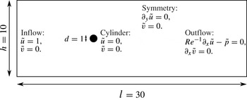
We apply the data-assimilation method described above to a simple test case: the two-dimensional flow around an infinite circular cylinder. Even though the theory was presented for a general three-dimensional flow, it applies straightforwardly to a two-dimensional case. The geometry, as well as the corresponding boundary conditions are presented in figure 1. We restate the boundary conditions of the direct system (2.4) for clarity:
 $$\begin{eqnarray}\left.\begin{array}{@{}l@{}}{\tilde{u}}=1,\quad \tilde{v}=0\quad \text{at the inlet},\\ {\tilde{u}}=0,\quad \tilde{v}=0\quad \text{on the cylinder's surface},\\ \partial _{y}{\tilde{u}}=0,\quad \tilde{v}=0\quad \text{on symmetry boundaries},\\ \mathit{Re}^{-1}\partial _{x}{\tilde{u}}-\tilde{p}=0,\quad \partial _{x}\tilde{v}=0\quad \text{at the outlet}.\end{array}\right\}\end{eqnarray}$$
The boundary conditions of the adjoint system (2.13) are obtained via the integration-by-parts step as explained in § 2.4. These conditions read
 $$\begin{eqnarray}\left.\begin{array}{@{}l@{}}{\tilde{u}}^{\dagger }=0,\quad \tilde{v}^{\dagger }=0\quad \text{at the inlet},\\ {\tilde{u}}^{\dagger }=0,\quad \tilde{v}^{\dagger }=0\quad \text{on the cylinder's surface},\\ \partial _{y}{\tilde{u}}^{\dagger }=0,\quad \tilde{v}^{\dagger }=0\quad \text{on symmetry boundaries},\\ \mathit{Re}^{-1}\partial _{x}{\tilde{u}}^{\dagger }+\tilde{p}^{\dagger }=-{\tilde{u}}{\tilde{u}}^{\dagger },\quad \mathit{Re}^{-1}\partial _{x}\tilde{v}^{\dagger }=-{\tilde{u}}\tilde{v}^{\dagger }\quad \text{at the outlet}.\end{array}\right\}\end{eqnarray}$$
Sketch of the geometry of two-dimensional flow around an infinite cylinder. The full computational domain, the characteristic lengths and the applied boundary conditions are shown. The cylinder’s diameter, the height and length of the domain
 $d$
,
 $h$
and
 $l$
are given in non-dimensional units.

This flow has been shown (see Jackson Reference Jackson1987) to undergo a first transition (more precisely, a supercritical Hopf bifurcation) at a critical Reynolds number of
 $\mathit{Re}_{c}\simeq 46$
, above which the base flow (solution of the system (2.4) with
 $\boldsymbol{f}=0$
) is no longer stable. Beyond this threshold, the flow becomes time periodic, and vortices are shed from the back of the cylinder. After this transition, we can define any mean quantity by averaging its instantaneous value over a finite number of periods in. By doing so, we can compute the mean-velocity field
 $\overline{\boldsymbol{u}}$
as well as the different components of the Reynolds stress tensor
 $\overline{\boldsymbol{u}_{i}^{\prime }\boldsymbol{u}_{j}^{\prime }}$
, defined in (2.2).
As we mentioned earlier, the optimization method employed in the remainder of this article requires the definition of an initial guess
 $\boldsymbol{f}_{g}$
for the forcing. We choose
 $\boldsymbol{f}_{g}=0$
, which means that the first computed flow
 $\tilde{\boldsymbol{u}}$
is the base flow
 $\boldsymbol{u}_{b}$
.
For our simulations, we choose a Reynolds number of
 $\mathit{Re}=150$
and compute the base flow
 $\boldsymbol{u}_{b}$
(using a classical Newton method), the mean flow
 $\overline{\boldsymbol{u}}$
(using time averaging) and the various components of the Reynolds stress tensor. These fields are computed with high accuracy using a finite-element method, using FreeFem
 $++$
software (see www.freefem.org), on a mesh of
 $N\simeq 1.7\times 10^{5}$
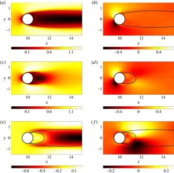
degrees of freedom. The base flow is represented in figure 2(a,b); the mean flow is displayed in figure 2(c,d) and finally the initial error is plotted in figure 2(e, f).
Flow around an infinite cylinder at
 $\mathit{Re}=150$
. (a) and (b) Base flow
 $\boldsymbol{u}_{b}$
; (c) and (d) time-averaged flow
 $\overline{\boldsymbol{u}}$
; (e) and ( f) Difference (evaluated on both components)
 ${\rm\Delta}\boldsymbol{u}$
, measuring the error committed when approximating the mean flow by the base flow. The left column represents the
 $x$
-component of the corresponding vector field, while the right column displays the
 $y$
-component. The dashed-lines refer for each vector-field to the extent of the recirculation bubble. The dashed lines of (a–d) have been reproduced in (e) and ( f) for comparison.

4. Navier–Stokes-driven field reconstruction
To validate the presented data-assimilation method, several measure operators
 $\mathscr{M}$
are considered, each of them chosen to demonstrate the efficacy of the method in various reconstruction scenarios. In the two following sections the considered measure is the full velocity vector and the error on both components of the velocity is estimated. Spatial interpolation and extrapolation are investigated. In a further section, we consider a more challenging and realistic case where only the velocity magnitude is measured, on a relatively coarse mesh. We demonstrate the ability of the method to not only reconstruct the measured quantity but also to identify the full velocity vector. The robustness of the identification algorithm when the measure is corrupted by noise is also assessed.
4.1. Full-state information identification
As a starting point, we will choose the operator
 $\mathscr{M}$
to be the identity operator on
 $V$
, such that the assimilated field is the full, continuous velocity field (in practice, it is a discrete field, evaluated on the finite-element grid). In this case, we choose
 $\langle \cdot ,\cdot \rangle _{M}\equiv \langle \cdot ,\cdot \rangle$
and
 $\Vert \cdot \Vert _{M}\equiv \Vert \cdot \Vert _{2}$
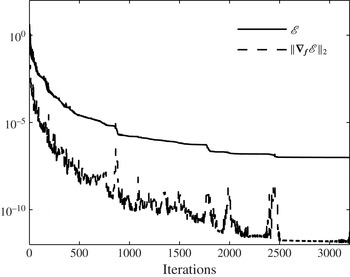
. We present the convergence curves for the case
 $\mathscr{M}=\mathscr{I}$
for both the cost functional
 $\mathscr{E}$
and the norm of the gradient
 $\boldsymbol{{\rm\nabla}}_{\boldsymbol{f}}\mathscr{E}$
in figure 3. It is seen that both quantities decrease by several orders of magnitude, indicating that the error
 $\mathscr{E}$
becomes extremely weak in the case of full-state information identification.
Convergence curves for full-identification case (
 $\mathscr{M}=\mathscr{I}$
). The solid line represents
 $\mathscr{E}$
,and the dashed line represents
 $\Vert \boldsymbol{{\rm\nabla}}_{\boldsymbol{f}}\mathscr{E}\Vert _{2}$
.

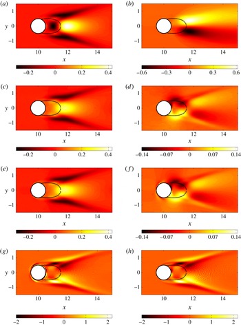
We plot in figure 4(a,b) both components of the true forcing
 $\boldsymbol{f}^{\ast }$
(computed via a DNS) and in figure 4(e, f) those related to the identified forcing
 $\boldsymbol{f}_{opt}$
. There exists a strong correlation for the streamwise component, but no similarity can be found for the cross-stream component. This was expected because the identification algorithm yields a forcing
 $\boldsymbol{f}_{opt}$
which is divergence-free while
 $\boldsymbol{f}^{\ast }$
is not. The divergence-free component of the latter forcing,
 $\boldsymbol{f}_{s}^{\ast }$
, is computed following the procedure explained in § 2.6 and we plot the results in figure 4(c,d). We can see that the identified forcing
 $\boldsymbol{f}_{opt}$
is indeed matching the projected forcing
 $\boldsymbol{f}_{s}^{\ast }$
. However, some discrepancies appear on the cylinder’s surface, which are due to the different tangential values of these two fields on the cylinder surface.
Averaged forcing term
 $\boldsymbol{f}^{\ast }$
displaying the
 $x$
and
 $y$
components, respectively, in (a) and (b). Projected forcing
 $\boldsymbol{f}_{s}^{\ast }$
(see § 2.6 for its definition) for both components, in (c) and (d). Optimally identified forcing
 $\boldsymbol{f}_{opt}$
for both components, in (e) and ( f). Note that the colour scales are identical for all streamwise components, but vary for the cross-stream components. However, (d) and ( f) have the same colour scale to allow comparison. Parts (g) and (h) represent the
 $z$
-component of
 $\boldsymbol{{\rm\nabla}}\times \boldsymbol{f}^{\ast }$
and
 $\boldsymbol{{\rm\nabla}}\times \boldsymbol{f}_{opt}$
, respectively. The difference is mainly located close to the cylinder’s surface. The dashed lines refer for each vector field to the extent of the recirculation bubble.

Differences between
 $\boldsymbol{f}_{opt}$
and the projection of
 $\boldsymbol{f}^{\ast }$
over the space of divergence-free fields are best analysed by comparing the curl of these two fields, since the curl of a potential field is zero. We can observe in figure 4(g,h) that the
 $z$
-component of these fields is nearly the same everywhere except in the vicinity of the cylinder boundary. We therefore have
 $\boldsymbol{f}_{opt}=\boldsymbol{f}_{s}^{\ast }$
almost everywhere, which validates our optimization procedure.
4.2. Partial-state information identification
In the case of a partial-state information identification, we still minimize
 $\mathscr{E}$
as defined in (2.5), expecting that this minimization results in a decrease of the real error
 ${\rm\Delta}\boldsymbol{u}$
(see (2.6)). We therefore need to decide how to measure the real error
 ${\rm\Delta}\boldsymbol{u}$
. We choose to use two norms: the
 $L^{2}$
-norm (normalized by
 $\sqrt{V_{{\it\Omega}}}$
to remove any dependence on the chosen area of integration) and the
 $L^{\infty }$
-norm. The first will give information about the average error while the second will yield the error at the worst reconstructed location. We therefore define the following residuals (measuring the real errors):
 $$\begin{eqnarray}\left.\begin{array}{@{}l@{}}r_{2}={\displaystyle \frac{1}{\sqrt{V_{{\it\Omega}}}}}\left\Vert {\rm\Delta}\boldsymbol{u}\right\Vert _{2}=\sqrt{{\displaystyle \frac{1}{V_{{\it\Omega}}}}\displaystyle \int _{{\it\Omega}}\left|{\rm\Delta}\boldsymbol{u}\right|^{2}\,\text{d}{\it\Omega}},\vspace{3.0pt}\\ r_{\infty }=\left\Vert {\rm\Delta}\boldsymbol{u}\right\Vert _{\infty }=\lim _{p\rightarrow +\infty }\displaystyle \left(\int _{{\it\Omega}}\left|{\rm\Delta}\boldsymbol{u}\right|^{p}\,\text{d}{\it\Omega}\right)^{1/p}.\end{array}\right\}\end{eqnarray}$$
4.2.1. Interpolation
Interpolation consists of reconstructing the field in between the available, measured data points. In what follows, the measure (as defined in (2.21)) is an average over each element of a rectangular mesh (called measurement mesh) and is reconstructed on the computational mesh which has a very high resolution. Here,
 $\mathscr{Q}$
is the identity operator, i.e. the two components of the velocity vector are measured:
 $$\begin{eqnarray}\mathscr{Q}\left(\tilde{\boldsymbol{u}}\right)=\tilde{\boldsymbol{u}}.\end{eqnarray}$$
In order to characterize the efficacy of the field reconstruction method, the discretization projection operator
 $\mathscr{P}$
defined in (2.21) is considered, with the
 $b_{i}$
being the basis functions of a mesh composed of squares paving the whole computational domain. The different measurement meshes have different line density (density per unit length) of points
 $n\in [2,20]$
. For instance, the case
 $n=2$
corresponds to
 $60\times 20$
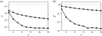
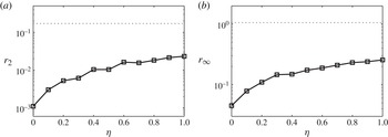
measurements meshes. An integrated measure is performed on each of the elements composing the measurement mesh, according to the expression (2.21). The identification algorithm is applied to all of the above measurement meshes and, for each optimum found, the errors
 $r_{2}$
and
 $r_{\infty }$
as defined in (4.1) are plotted against the line-density of points
 $n$
in figure 5.
Results for the interpolation case: (a)
 $r_{2}$
error; (b)
 $r_{\infty }$
error as defined in (4.1). The norm of the error is plotted against the line density of nodes
 $n$
. Circle symbols represent the spline interpolation case (naïve approach) and square symbols represent the data-assimilation results. The error of approximating the mean flow by the base flow is represented with a dashed line. For
 $n\simeq 10$
, the reconstruction of the field is efficient and a further increase of resolution yields only little improvement.

First, it is encouraging that even for the worst case considered (
 $n=2$
), the reconstructed mean flow corresponds to a relatively low error. The measure
 $\mathscr{M}(\overline{\boldsymbol{u}})$
performed in a particularly under-resolved case (
 $n=2$
) as well as the corresponding reconstructed field
 $\tilde{\boldsymbol{u}}_{opt}$
and error
 ${\rm\Delta}\boldsymbol{u}$
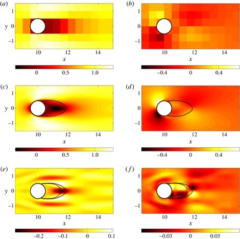
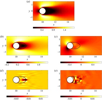
are plotted in figure 6. From this figure, we can confirm that the data-assimilation algorithm successfully identifies the mean field. Indeed, for this extremely coarse case, the
 $L^{2}$
error is
 $r_{2}=0.012$
, which is very small considering the amount of information initially given. However, the maximum error is
 $r_{\infty }=0.297$
. We have found an average error of 1.2 %, and of 29.7 % at the worst reconstructed location. Both of these errors are relative to the unit inflow velocity. We see in figure 6(e, f) that the error is mainly located in the near-wake of the cylinder. The worst-reconstructed area corresponds to the end of the recirculation bubble whose reattachment point location does not exactly match the real one (extracted from the mean flow
 $\overline{\boldsymbol{u}}$
); its length is underestimated by the identification algorithm. For more accurate measures (increasing
 $n$
), the error decreases: the more information is available initially, the more accurately the field is reconstructed. For the finest meshes, we can reduce the errors to
 $6.36\times 10^{-3}\%$
in
 $L^{2}$
-norm and 0.17 % in
 $L^{\infty }$
-norm.
Measures of the two velocity components: (a)
 $\mathscr{M}(\overline{u})$
; (b)
 $\mathscr{M}(\overline{v})$
. The measurement corresponds to a rectangular mesh of line density of points
 $n=2$
, and the measurement window is the full flow field. Reconstructed fields: (c)
 ${\tilde{u}}$
; (d)
 $\tilde{v}$
. Error fields: (e)
 ${\rm\Delta}u$
; ( f)
 ${\rm\Delta}v$
. The dashed lines in (c) and (d) refer to the extent of the recirculation bubble of the reconstructed field. These dashed lines have been reproduced in (e) and ( f), along with those of the true mean flow.

Spline interpolation is a non-physical, but common way to obtain highly refined fields from measurements on a coarse grid. To assess the improved quality of data-assimilation interpolation, figure 5 also presents the interpolation error for a classical spline interpolation reconstruction. We note that this simple interpolation technique is producing better results than a base-flow approximation, but is far from being as accurate as the presented algorithm. The data-assimilation method always outperforms spline interpolation and can lead to more accurate results by two orders of magnitude.
4.2.2. Extrapolation
In this section, the operator defining the measured quantity is still the identity (
 $\mathscr{Q}=\mathscr{I}$
), i.e. the full velocity vector is assimilated on a given measurement mesh. However, the projection operator
 $\mathscr{P}$
is now designed to investigate the extrapolation capabilities of the method. The used mesh is the finer one from the previous section (the line density of points is
 $n=20$
), but locations, where measurements are performed, are limited in space. More precisely, the assimilation (or identification) window has the height of the computational domain but varies in length. For a given abscissa
 $x_{0}$
, we consider two different identification windows: the first starting at
 $x=5$
and ending at
 $x=x_{0}$
, and the second starting at
 $x=x_{0}$
and ending at
 $x=25$
. The two identification windows are thus
 $W_{1}=[5,x_{0}]$
and
 $W_{2}=[x_{0},25]$
.
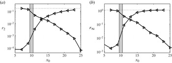
The results are presented in figure 7. The first series of simulations for the identification window
 $W_{1}=[5,x_{0}]$
shows that the error is decreasing with the length of the identification window. The algorithm starts to produce accurate results as soon as the zone around the cylinder is included in the assimilation window (from
 $x_{0}=11$
). In particular, if the data assimilated does not contain any measures where the mean flow and base flow are different (unsteady zones), the identification will not be able to match the mean flow, since hardly any information is provided. However, as soon as some unsteady zones are assimilated, the algorithm is able to reconstruct not only the identified zone, but the full flow field. This demonstrates that extrapolation is a true capability of the presented data-assimilation method. The second series of simulations corresponds to the identification window
 $W_{2}=[x_{0},25]$
. In this case, even for small identification windows (starting from
 $x_{0}=23$
), the mean and base flows are different in the considered zone. Therefore, the extrapolation is relatively effective, even with little information, as we can see by considering the
 $L^{2}$
-norm plot of the error (figure 7
a). However, the
 $L^{\infty }$
residual
 $r_{\infty }$
remains rather large (see figure 7
b).
Results for the extrapolation case: (a)
 $r_{2}$
error; (b)
 $r_{\infty }$
error as defined in (4.1). The error
 $\Vert {\rm\Delta}\boldsymbol{u}\Vert$
is plotted against the streamwise coordinate
 $x_{0}$
defining the extent of the identification window. Right-oriented triangles are associated with the measurement window
 $W_{1}=[5,x_{0}]$
, while the left-oriented triangles correspond to the identification window
 $W_{2}=[x_{0},25]$
. The error of approximating the mean flow by the base flow is represented by a dashed line. The grey rectangle represents the location of the cylinder.

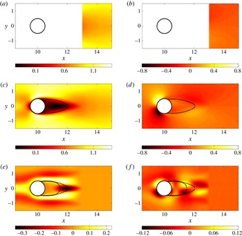
Measures of the two velocity components: (a)
 $\mathscr{M}(\overline{u})$
; (b)
 $\mathscr{M}(\overline{v})$
. The measurement corresponds to a rectangular mesh of line density of points
 $n=20$
and the measurement window is
 $W_{2}=[13,25]$
(
 $x_{0}=13$
). Reconstructed fields: (c)
 ${\tilde{u}}$
; (d)
 $\tilde{v}$
. Error fields: (e)
 ${\rm\Delta}u$
; ( f)
 ${\rm\Delta}v$
. The dashed lines in (c) and (d) refer to the extent of the recirculation bubble of the reconstructed field. These dashed lines have been reproduced in (e) and ( f), along with those of the true mean flow.

The results of the extrapolation for the identification window
 $W_{2}=[13,25]$
(corresponding to
 $x_{0}=13$
) are presented in figure 8. We can see that only limited information is available downstream of the cylinder; in particular, the location of the reattachment point of the recirculation bubble is outside the identification window. Despite this lack of information, the reconstructed field
 $\tilde{\boldsymbol{u}}$
is very similar to the mean flow
 $\overline{\boldsymbol{u}}$
. However, some non-negligible errors in the reconstruction appear immediately upstream of the identification window (nearly no error can be found within the identification window). Interestingly, the incoming flow field has been modified from a uniform flow to a
 $y$
-dependent flow field (the uniform inflow boundary condition is still satisfied further upstream), as we can see in figure 8(c), illustrating that several types of solutions can be found depending on the quality of the measure. In fact, it is likely that the cost functional is multimodal (several local minima may exist), associated with different flow fields, one of which is the physical solution of the problem. There is however no guarantee, as demonstrated here, of finding this physical solution. Nevertheless, even if the mean flow is not exactly matched, the reconstructed field yields far more information about the nature of the flow than is contained in the initial information we measured.
The results of the extrapolation procedure indicate that the field is best reconstructed as long as the recirculation bubble is part of the measurement window. This finding is reminiscent of the results by Marquet, Sipp & Jacquin (Reference Marquet, Sipp and Jacquin2008) and Pralits, Brandt & Giannetti (Reference Pralits, Brandt and Giannetti2010) who showed that the recirculation bubble is the most sensitive region regarding the overall dynamics of the flow field.
4.2.3. State vector reconstruction
In order to approach real cases for which this method is likely to be employed, we proceed from the full two-component velocity matching to a scalar-field matching based on the velocity magnitude. The operator defining the measured quantity is therefore
 $$\begin{eqnarray}\mathscr{Q}(\boldsymbol{u})={\textstyle \frac{1}{2}}\left|\boldsymbol{u}\right|^{2}={\textstyle \frac{1}{2}}\left(u^{2}+v^{2}\right).\end{eqnarray}$$
The projection operator
 $\mathscr{P}$
is chosen such that the measure domain is the entire domain and the line density of points of the measures is
 $n=6$
. The measured field
 $\tilde{\boldsymbol{m}}$
is plotted in figure 9(a). The reconstructed field from data assimilation of the measurements is presented in figure 9(b,c).
(a) Velocity magnitude measures on a mesh corresponding to
 $n=6$
. (b) and (c) Reconstructed field
 $\boldsymbol{u}_{opt}$
. (d) and (e) Two components of the error
 ${\rm\Delta}\boldsymbol{u}$
. The dashed lines in (b) and (c) represent the extent of the recirculation bubble for the reconstructed field. These lines have been reproduced in (d) and (e), along with those of the true recirculation bubble.

We observe that even though only velocity magnitude on a rather coarse mesh has been used as an input to our data-assimilation algorithm, it is possible to retrieve a good approximation of the full component-wise mean-velocity field. Both the streamwise and normal velocity components have been recovered accurately, with a small error concentrated around the recirculation zone in the near-wake of the cylinder.
4.3. Noise reduction
Experimental measurements are often contaminated by noise, and for an application of data assimilation to experimental data the ability of the technique to deal with measurement noise must be studied. We consider the same measure operator
 $\mathscr{M}$
as presented in the previous section: velocity magnitude measured on a mesh of line density
 $n=6$
. We thus have
 $\boldsymbol{m}^{\ast }=\mathscr{M}(\overline{\boldsymbol{u}})$
where the asterisk indicates a noiseless quantity. We add to this measure a noise component
 $$\begin{eqnarray}\overline{\boldsymbol{m}}=\boldsymbol{m}^{\ast }+{\it\eta}{\it\xi},\end{eqnarray}$$
with
 ${\it\xi}$
a random
 $N$
-dimensional vector and
 ${\it\eta}$
a real number controlling the amplitude of the added noise. The vector
 ${\it\xi}$
is constructed with a uniform distribution chosen such that
 $|{\it\xi}_{i}|<\sqrt{\Vert \boldsymbol{m }^{\ast }\Vert _{M}^{2}/N}$
. The level of noise is governed by the real number
 ${\it\eta}$
; for example,
 ${\it\eta}=0.1$
corresponds to a noise-to-signal ratio of 10 %, while for
 ${\it\eta}=1$
we have a 100 % noise-to-signal ratio. These ratios depend on the norm used to define the noise, in our case, the
 $L^{2}$
-norm. We present in figure 10 the results of data assimilation as a function of the noise level
 ${\it\eta}$
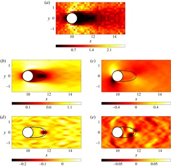
. The error is, as expected, an increasing function of the noise level. The algorithm however captures the flow features very well, even for large noise amplitudes. The measure, the reconstructed field and the error are plotted in figure 11 for
 ${\it\eta}=1$
. The identified field
 $\tilde{\boldsymbol{u}}$
is also relatively noisy, but the flow has been remarkably reconstructed from a low-resolution, scalar and noisy measure. Moreover, the recirculation bubble is accurately reconstructed, together with the main features of the flow.
Results for the noise reduction case: (a)
 $r_{2}$
error; (b)
 $r_{\infty }$
error as defined in (4.1). The error (measured relative to the base flow error)
 $\Vert {\rm\Delta}\boldsymbol{u}\Vert$
is plotted (square symbols) against the noise strength
 ${\it\eta}$
in the measured signal. The error made by approximating the mean flow by the base flow is represented with a dashed line.

(a) Velocity magnitude measures on a mesh corresponding to
 $n=6$
. The noise level has been set to
 ${\it\eta}=1$
, i.e. we have a 100 % noise-to-signal ratio according to our definition. (b) and (c) Reconstructed field
 $\boldsymbol{u}_{opt}$
. (d) and (e) Two components of the error
 ${\rm\Delta}\boldsymbol{u}$
. The dashed lines in (b) and (c) refer to the extent of the recirculation bubble of the reconstructed field. These dashed lines have been reproduced in (d) and (e), along with those of the true mean flow.

The evolution, during the iterative process, of both the cost functional
 $\mathscr{E}$
and the real
 $L^{2}$
residual
 $r_{2}$
for the two cases,
 ${\it\eta}=0$
(no noise) and
 ${\it\eta}=1$
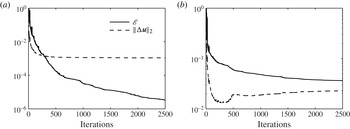
(noise level of 100 %), are plotted in figure 12. We can see that for both cases, the cost functional
 $\mathscr{E}$
decreases monotonically (due to the gradient descent), but reaches an asymptote at a higher value for the noisy case, confirming that it is not possible to match the measurement noise with a solution of the Navier–Stokes equations. The Navier–Stokes operator thus acts as a filter and cannot provide a fit matching the noise-corrupted measurement. Analysing the evolution of
 $r_{2}$
, we see that in the noiseless case the real error monotonically decreases, while it starts to decrease and then increases again, after approximately 200 iterations, for the noisy measurements case. This means that after the turning point, the algorithm tries to match the measurement noise, which drives the solution away from the physical solution
 $\overline{\boldsymbol{u}}$
. In a real situation, this convergence curve is not accessible, and we therefore cannot terminate the iterative identification when the error is lowest. It is however useful to evaluate when to stop the reconstruction based on a comparison between the norm of the gradient of the cost functional and an estimation of the measurement noise level.
(a) Convergence curves for the noiseless case (
 ${\it\eta}=0$
) and (b) for the noisiest case (
 ${\it\eta}=1$
). We note that for the case without noise, both the cost functional
 $\mathscr{E}$
and the real residual
 $r_{2}$
are monotonically decreasing. For the noisy case, however, even though
 $\mathscr{E}$
decreases as a result of the optimization, around the 200th iteration, the real residual
 $r_{2}$
starts to increase again, signifying that from this point forward the optimization actually leads to a deterioration of the identified optimal mean flow
 $\tilde{\boldsymbol{u}}$
.

5. Additional flow reconstruction
5.1. Drag evaluation
Another way to assess the quality of the reconstructed fields is to compare the cylinder drag of the mean field with the drag of the reconstructed field. The drag coefficient
 $C_{D}$
induced by a field
 $(\boldsymbol{u},p)^{\top }$
on the cylinder is defined as
 $$\begin{eqnarray}C_{D}=\underbrace{2\int _{\mathscr{C}}\mathit{Re}^{-1}\left(\boldsymbol{{\rm\nabla}}\boldsymbol{u}+\boldsymbol{{\rm\nabla}}\boldsymbol{u}^{\top }\right)\boldsymbol{n}\boldsymbol{\cdot }\boldsymbol{e}_{x}\,\text{d}l}_{C_{V}}+\underbrace{2\int _{\mathscr{C}}-p\boldsymbol{n}\boldsymbol{\cdot }\boldsymbol{e}_{x}\,\text{d}l}_{C_{P}},\end{eqnarray}$$
where
 $\mathscr{C}$
represents the cylinder’s surface and
 $\text{d}l$
the integration element along this contour. The factors 2 stem from the normalization by the dynamic pressure
 ${\textstyle \frac{1}{2}}{\it\rho}U^{2}$
, which simplifies to
 ${\textstyle \frac{1}{2}}$
in the non-dimensional variables. As seen in (5.1), we can divide the drag force into two components: the viscous drag
 $C_{V}$
and the pressure drag (or form drag)
 $C_{P}$
. We expect the
 $C_{V}$
-component to be accurately predicted (as it only depends on the velocity vector which is properly reconstructed), and the
 $C_{P}$
-component to exhibit a more appreciable mismatch (as the true pressure field
 $\bar{p}$
is only recovered up to a scalar field
 ${\it\phi}$
linked to the potential part of the Reynolds stress term, as explained in (2.29)).
We display in table 1 the different drag coefficients obtained for the true mean flow
 $(\bar{\boldsymbol{u}},\bar{p})^{\top }$
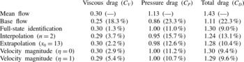
and for several reconstruction scenarios. We note that, as expected, the viscous drag is accurately predicted whereas the relative error on the pressure drag is always greater than 10 %. Note that for larger Reynolds numbers, the viscous drag is expected to decrease and, therefore, the relative total error to increase.
Drag coefficients for the mean flow obtained through DNS simulation, for the base flow, for the full-state identification and for several reconstruction scenarios corresponding to the cases displayed in figures 6, 8, 9 and 11. The relative error with respect to the mean flow is displayed in parentheses for each case.

5.2. Unsteadiness characterization
In the previous sections, we have exploited the reconstruction abilities of the data-assimilation technique by analysing the reconstructed state vector for several cases of interest. In this section, we explore the possibilities of unsteadiness characterization offered by the identified forcing
 $\boldsymbol{f}_{opt}$
in the case of full-state information identification, where the global optimal has been reached.
As covered in § 2.6, the algorithm only identifies the solenoidal part of the true forcing
 $\boldsymbol{f}^{\ast }=-\boldsymbol{{\rm\nabla}}\boldsymbol{\cdot }\unicode[STIX]{x1D64D}$
. However, it is the full Reynolds stress tensor
 $\unicode[STIX]{x1D64D}$
, rather than the components of its divergence, that would be most valuable. In a two-dimensional setting, this tensor can be expressed as
 $$\begin{eqnarray}\unicode[STIX]{x1D64D}=\left(\begin{array}{@{}cc@{}}{\it\alpha} & {\it\beta}\\ {\it\beta} & -{\it\alpha}\end{array}\right)+k\boldsymbol{I},\end{eqnarray}$$
with
 ${\it\alpha}={\textstyle \frac{1}{2}}(\overline{u^{\prime 2}}-\overline{v^{\prime 2}})$
,
 ${\it\beta}=\overline{u^{\prime }v^{\prime }}$
and
 $k={\textstyle \frac{1}{2}}(\overline{u^{\prime 2}}+\overline{v^{\prime 2}})$
denoting the fluctuating kinetic energy. These quantities vanish on the cylinder’s surface due to the no-slip boundary condition.
It should then be possible to optimally reconstruct a tensor of this particular structure from the identified forcing
 $\boldsymbol{f}_{opt}$
. As we explained in § 2.6, the forcing
 $\boldsymbol{f}^{\ast }$
can be decomposed into a solenoidal part and a potential component as
 $\boldsymbol{f}^{\ast }=\boldsymbol{f}_{s}^{\ast }+\boldsymbol{{\rm\nabla}}{\it\phi}$
. Furthermore, we also have
 $\boldsymbol{f}_{s}^{\ast }\simeq \boldsymbol{f}_{opt}$
(strict equality is not true because of the boundary condition issue discussed in § 2.6). In summary, we have
 $$\begin{eqnarray}\displaystyle \boldsymbol{f}^{\ast } & = & \displaystyle -\left(\begin{array}{@{}c@{}}\partial _{x}{\it\alpha}+\partial _{y}{\it\beta}\\ \partial _{x}{\it\beta}-\partial _{y}{\it\alpha}\end{array}\right)-\boldsymbol{{\rm\nabla}}k\end{eqnarray}$$
 $$\begin{eqnarray}\displaystyle & \simeq & \displaystyle \boldsymbol{f}_{opt}+\boldsymbol{{\rm\nabla}}{\it\phi}.\end{eqnarray}$$
 ${\it\alpha}$
,
 ${\it\beta}$
and the identified forcing
 $\boldsymbol{f}_{opt}$
. Such an identification, however, is under-constrained as we have only one equation for two unknowns. If we further assume that
 $-\boldsymbol{{\rm\nabla}}k\simeq \boldsymbol{{\rm\nabla}}{\it\phi}$
(see the next section for justification in the cylinder case), we obtain
 $$\begin{eqnarray}-\left(\begin{array}{@{}c@{}}\partial _{x}{\it\alpha}+\partial _{y}{\it\beta}\\ \partial _{x}{\it\beta}-\partial _{y}{\it\alpha}\end{array}\right)=\boldsymbol{f}_{opt}.\end{eqnarray}$$
This yields two equations for two unknowns, along with the boundary conditions
 ${\it\alpha}=0$
and
 ${\it\beta}=0$
on the boundaries. Yet, recalling that the optimal forcing is divergence-free (
 $\boldsymbol{{\rm\nabla}}\boldsymbol{\cdot }\boldsymbol{f}_{opt}=0$
), we obtain a constraint on
 ${\it\alpha}$
and
 ${\it\beta}$
, which is non-physical so that the identified
 ${\it\alpha}$
and
 ${\it\beta}$
obtained by solving (5.4) will, in general, not match their experimental values. Instead, we propose a weaker constraint to relate the left- and right-hand sides of (5.4). We decide in the following to minimize the cost functional
 $$\begin{eqnarray}\mathscr{I}({\it\alpha},{\it\beta})=\int _{{\it\Omega}}((-\partial _{x}{\it\alpha}-\partial _{y}{\it\beta}-f_{x})^{2}+(-\partial _{x}{\it\beta}+\partial _{y}{\it\alpha}-f_{y})^{2})\,\text{d}{\it\Omega},\end{eqnarray}$$
where
 $\boldsymbol{f}_{opt}=(\,f_{x},f_{y})$
. This minimization problem is solved by setting the gradient of this cost functional to zero. This leads to the two independent equations
 $$\begin{eqnarray}\displaystyle & {\rm\nabla}^{2}{\it\alpha}=-\partial _{x}\,f_{x}+\partial _{y}\,f_{y}, & \displaystyle\end{eqnarray}$$
 $$\begin{eqnarray}\displaystyle & {\rm\nabla}^{2}{\it\beta}=-\partial _{y}\,f_{x}-\partial _{x}\,f_{y}, & \displaystyle\end{eqnarray}$$
Results for (a)
 ${\it\alpha}$
and (b)
 ${\it\beta}$
of the real reduced Reynolds stress tensor, and reconstructed tensor components (c)
 ${\it\alpha}_{opt}$
and (d)
 ${\it\beta}_{opt}$
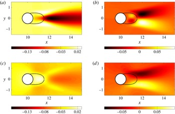
. The dashed lines indicate the extent of the recirculation bubble of the true mean flow.

We see in this figure that the reconstruction of the coefficients which characterize the unsteadiness of the flow fails for
 ${\it\alpha}$
but yields relatively good results for
 ${\it\beta}$
.
5.3. Pressure reconstruction
The component of the reconstructed field that we have not yet analysed, is the pressure
 $\tilde{p}_{opt}$
. We know that the optimally identified pressure
 $\tilde{p}_{opt}$
is the difference between the real mean pressure
 $\overline{p}$
and the potential
 ${\it\phi}$
(see (2.29)). It is interesting to compare the reconstructed pressure field
 $\tilde{p}_{opt}$
to the base-flow pressure
 $p_{b}$
(for sake of comparison), to the real mean pressure
 $\overline{p}$
and to the total pressure
 $p_{T}=\overline{p}+k$
(sum of the real mean pressure and the fluctuating kinetic energy
 $k$
). This is achieved in figure 14.
(a) Base-flow pressure
 $p_{b}$
; (b) mean flow pressure
 $\overline{p}$
; (c) total pressure
 $p_{T}=\overline{p}+k$
; (d) reconstructed pressure
 $\tilde{p}_{opt}$
. The dashed-lines indicate the extent of the recirculation bubbles, (a) in the case of the base flow, (b–d) in the case of the true mean flow.

Analysing the base-flow pressure
 $p_{b}$
and the real mean pressure
 $\overline{p}$
, we note that the pressure drop is centred on the respective recirculation bubbles. However, the real mean pressure also displays a constant pressure drop in the wake of the cylinder. If we consider the total pressure
 $p_{T}$
, we can see that this wake effect disappears and the pressure drop appears to be mainly located within the recirculation bubble. When compared with the reconstructed pressure
 $\tilde{p}_{opt}$
, we can see that the two pressure fields
 $p_{T}$
and
 $\tilde{p}_{opt}$
are very similar, even though the reconstructed pressure is slightly overestimated near the end of the recirculation bubble, around the stagnation point. The difference between these two pressure fields is weak, so that
 $-k\simeq {\it\phi}$
, therefore justifying the assumption
 $-\boldsymbol{{\rm\nabla}}k\simeq \boldsymbol{{\rm\nabla}}{\it\phi}$
of the previous section. It is remarkable that the pressure reconstructed from velocity measurements only
 $\tilde{p}_{opt}$
, is rather close to the total pressure
 $p_{T}$
, and also not that far from the real pressure
 $\overline{p}$
. In order to improve the identification of the real mean-pressure field, it is mandatory to incorporate pressure measurements within the data-assimilation algorithm. This is briefly discussed below.
6. Concluding remarks and extensions
Despite recent progress in experimental measuring techniques, many data from experiments are still limited in terms of resolution, in terms of access to specific regions of interest and in terms of quantities that can be measured reliably. We have developed and introduced a data-assimilation technique for the recovery of mean flow fields that are solutions of the RANS equations and match the available data points. The algorithm, based on an iterative, direct-adjoint optimization approach, has been validated on two-dimensional flow past a circular cylinder at a supercritical Reynolds number (
 $\mathit{Re}=150$
). The method has been used in an interpolatory mode (recovering mean-velocity fields from much coarser measurements), in an extrapolatory mode (extending the mean-velocity field into domains where no measurements have been taken), and in a state-vector reconstruction mode (determining mean-velocity components from measurements of only the magnitude). In all cases, we have observed a satisfactory recovery of the mean-velocity field that proves substantially more accurate than more naïve approaches based on higher-order interpolation that disregard physical constraints on the mean fields. Moreover, the influence of noise in the input data fields has been assessed, and the method has been found to be robust, even in the face of a noise-to-signal ratio of 100 %.
Together with the assimilated mean-velocity field, we also obtain the forcing vector field that renders the error between the available measurements and the recovered mean-velocity field minimal. From this forcing, information about the unsteadiness and the pressure field can be extracted. However, this information is limited to the solenoidal part of the Reynolds stress tensor and the non-kinetic part of the pressure. Despite this limitations, it has to be kept in mind that only steady (averaged) information has entered the data-assimilation algorithm. Yet, we were able to gain insight, albeit partial and incomplete, on the second-order moments of the unsteady flow. This is quite remarkable, given the limited input information.
Various extensions and variations of the presented algorithms are conceivable. For large-Reynolds-number applications, the current numerical technique can be adapted to aid in the solving of (2.4) (which can be challenging for large Reynolds numbers when using Newton’s iteration method). Due to the averaging, we know that the mean flow will be similar to a base flow at a lower Reynolds number. We therefore propose to artificially decrease the Reynolds number in (2.4). Ideally one would choose the Reynolds number yielding a base flow as close as possible to the measured mean flow. We therefore have
 $\mathit{Re}=\mathit{Re}^{\ast }-{\rm\Delta}\mathit{Re}$
with
 $\mathit{Re}^{\ast }$
as the real flow Reynolds number and
 ${\rm\Delta}\mathit{Re}\ (0<{\rm\Delta}\mathit{Re}<\mathit{Re}^{\ast })$
as the adjustment performed. We can start with a zero initial guess (
 $\boldsymbol{f}_{g}=0$
) and identify the optimal forcing
 $\boldsymbol{f}_{opt}$
. The identified total forcing (for the Navier–Stokes equation with the given Reynolds number
 $\mathit{Re}^{\ast }$
) takes the form
 $\boldsymbol{f}_{opt}^{\ast }=\boldsymbol{f}_{opt}+({\rm\Delta}\mathit{Re}/\mathit{Re}\mathit{Re}^{\ast }){\rm\nabla}^{2}\tilde{\boldsymbol{u}}_{opt}$
, where we have added the contribution due to the artificial decrease of Reynolds number. We note that this method does not violate the divergence-free forcing condition. This technique can be thought of as a preconditioning method allowing us to bypass the problem of solving the Navier–Stokes equations for high Reynolds numbers. It can also be interpreted as a preconditioning step for the optimization. The initial guess
 $\boldsymbol{f}_{\boldsymbol{g}}$
could also be obtained by a RANS model (based, for example, on an eddy-viscosity closures or more elaborate Reynolds stress models). Indeed, by so proceeding we avoid the costly (and probably ill-posed) computation of a high-Reynolds-number base flow. Moreover, it is also possible to compare the Reynolds stresses issued from the turbulence model with those of the optimal solution compatible with the experimental observations. This approach would be interesting and useful in assessing the performance of turbulence closures in more complex flow configurations.
The cost functional, i.e. the error between measured and the model-predicted data can be augmented by a weight function which directs more emphasis towards regions that are of more relevance. For example, shear layers or regions close to walls can be singled out as more important and as having a larger contribution to the cost functional. Also, pressure measurements could be considered, leading to a more well-posed optimization problem as explained in § 2.6. Some of these extensions will be pursued in a future study. In its current form, the data-assimilation method is a very valuable tool for the experimentalist to recover more information about the flow than is directly measurable. In this sense, it takes the measured data beyond their intrinsic information content and extends the scope of current measurement capabilities.