Introduction
Water pollution by nitrate is one of the major consequences of intensive production systems in agricultural catchments (Carpenter et al., Reference Carpenter, Caraco, Correll, Howarth, Sharpley and Smith1998). Agricultural intensification results from the widespread specialization of agriculture which concentrates agricultural activities, here livestock production, in the same area, generating large nutrient surpluses (Billen et al., Reference Billen, Beusen, Bouwman and Garnier2010). Specialization and intensification are linked to economic drivers (Krugman, Reference Krugman1998; Grizzetti et al., Reference Grizzetti, Bouraoui and De Marsily2008; Bagoulla et al., Reference Bagoulla, Chevassus-Lozza, Daniel and Gaigné2010; Peyraud et al., Reference Peyraud, Cellier, Aarts, Béline, Bockstaller, Bourblanc, Delaby, Dourmad, Dupraz, Durand, Faverdin, Fiorelli, Gaigné, Kuikman, Langlais, Le Goffe, Lescoat, Morvan, Nicourt, Parnaudeau, Rochette, Vertès, Veysset, Réchauchère and Donnars2014). The mitigation measures are well known and well detailed at field, farm and catchment scale (Schoumans et al., Reference Schoumans, Chardon, Bechmann, Gascuel-Odoux, Hofman, Kronvang, Litaor, Lo Porto, Newell and Rubaek2011). The optimization of agricultural practices, whether through the reduction of inputs (Chaplot et al., Reference Chaplot, Saleh, Jaynes and Arnold2004; Zammit et al., Reference Zammit, Sivapalan, Kelsey and Viney2005; De Girolamo and Porto, Reference De Girolamo and Lo Porto2012; Qu and Kroeze, Reference Qu and Kroeze2012) or by limiting nitrogen leaching (e.g. with a catch crop) (Laurent and Ruelland, Reference Laurent and Ruelland2011), does not always achieve the 50 mg/l nitrate concentration targets of the Nitrate Directive (Arheimer et al., Reference Arheimer, Andersson, Larsson, Lindström, Olsson and Pers2004) in a context of intensive livestock production with high nutrient surplus (Durand, Reference Durand2004; Worrall et al., Reference Worrall, Spencer and Burt2009; Kay et al., Reference Kay, Grayson, Phillips, Stanley, Dodsworth, Hanson, Walker, Foulger, McDonnell and Taylor2012).
The management of landscape as a lever to reduce nitrogen (N) fluxes ranges from the implementation of grass strips, hedgerows or riparian buffers (Vache et al., Reference Vache, Eilers and Santelmann2002; Blanco-Canqui et al., Reference Blanco-Canqui, Gantzer, Anderson, Alberts and Thompson2004; Ferrant et al., Reference Ferrant, Durand, Justes, Probst and Sanchez-Perez2013) to conversion of parts of the catchment to forestry or unmanaged grasslands (Tian et al., Reference Tian, Huang and Xiao2010). Such measures may have additional benefits such as a protection against soil erosion (Da Silva et al., Reference Da Silva, Silva and De Souza2016), improving biodiversity (Burel and Baudry, Reference Burel and Baudry2003; Schulz and Schröder, Reference Schulz and Schröder2017) or phosphorus pollution mitigation (Farkas et al., Reference Farkas, Beldring, Bechmann and Deelstra2013). In the case of nitrate pollution, their effectiveness relies on two types of processes, i.e. (i) the decrease of the overall N input load on a given zone by decreasing the fertilized area, which can be assimilated as a dilution effect (in the sense of less pollutant for the same amount of water), and (ii) the interception, which means either retention or transformation of the nitrogen already lost by the agricultural land and circulating as solute. Grass strips, narrow riparian buffers or hedgerows activate mainly this interception effect, whereas land use conversion relies mainly on the dilution effect. In the first case, the efficiency of intercepting structures has been mostly assessed by local measurements and experiments, but such studies are difficult to generalize at the landscape scale because the effects are strongly site-specific (Burt et al., Reference Burt, Pinay and Sabater2010). In particular, it is likely that poor spatial targeting of interception structures may reduce their effect towards a mere diluting effect. In the second case, the conversion of part of the agricultural area into unfertilized vegetation has been assessed using global or semi-distributed models, with the underlying assumption that their precise location within the landscape has little effect on their efficiency. Arguably, locating land use conversion between the agricultural fields and the water bodies may combine dilution and interception effects. This remains uncertain, however, since many studies suggest that most of the N retention processes occur near the edges of the buffers or in hot spots, i.e. that their linear dimension or their heterogeneity are more important than their area (Burt et al., Reference Burt, Pinay and Sabater2010). It is therefore essential to better quantify these effects and improve knowledge on the optimal design of such landscape management (location, area, shape…). To do this, explicitly distributed biophysical models are useful tools, because of their ability to simulate the effect of located changes in land management (Jakeman and Letcher, Reference Jakeman and Letcher2003; Cherry et al., Reference Cherry, Shepherd, Withers and Mooney2008; Moreau et al., Reference Moreau, Ruiz, Raimbault, Vertes, Cordier, Gascuel-Odoux, Masson, Salmon-Monviola and Durand2012, Reference Moreau, Viaud, Parnaudeau, Salmon-Monviola and Durand2013). In particular, they are necessary to test ex ante a diversity of scenarios and to identify the impacts of the different strategies on the water and N cycles.
The current paper presents a modelling study of different N pollution mitigation strategies in a small catchment in western France. The main objectives were (1) to evaluate relative effectiveness and possible complementarity of field-oriented, interception-oriented and dilution-oriented measures to reduce N emissions, (2) to detail the controlling factors and their operational consequences in terms of landscape management. Agri-environmental scenarios of N management were built and applied in the Naizin–Kervidy study site (Brittany, France) and their effects on N emissions as nitrate and nitrous oxide (N2O) were assessed using the Topography Nitrogen Transfer and Transformation (TNT2) distributed model (Beaujouan et al., Reference Beaujouan, Durand, Ruiz, Aurousseau and Cotteret2002).
Materials and methods
Study site
The Naizin–Kervidy is a headwater catchment located in Brittany, Western France (48°N, 3°W), with long-term and high-frequency monitoring (AgrHys long-term research observatory). The catchment is part of the SOERE RBV (French Network of observatories: http://portailrbv.sedoo.fr/). As a result, it has been studied extensively, especially for soil properties, hydrology and biogeochemistry and farm/field N balances (Molénat et al., Reference Molénat, Durand, Gascuel-Odoux, Davy and Gruau2002, Reference Molénat, Gascuel-Odoux, Aquilina and Ruiz2013; Durand, Reference Durand2004; Payraudeau et al., Reference Payraudeau, Van Der Werf and Vertes2007; Aubert et al., Reference Aubert, Gascuel-Odoux, Gruau, Akkal, Faucheux, Fauvel, Grimaldi, Hamon, Jaffrézic, Lecoz-Boutnik, Molénat, Petitjean, Ruiz and Merot2013; Benhamou et al., Reference Benhamou, Salmon-Monviola, Durand, Grimaldi and Merot2013). Most of the data collected are available online (https://www6.inra.fr/ore_agrhys_eng/).
It is an intensive farming catchment of 4.82 km2 with 0.91 of agricultural area (AA) characterized by mixed farming. Dairy production, indoor pig breeding and poultry result in a high livestock density of about 5 livestock units (LSU)/ha. The main crop rotations consist of winter cereals, maize, grazing ley and vegetables. The climate is temperate oceanic with a mean day temperature of 11.2 °C (data from 2002 to 2015). Mean annual rainfall is 827 mm/year, with a minimum and a maximum monthly average reached in June (43 mm) and November (109 mm), respectively. The outlet is a second Strahler order stream, which usually dries out in summer. The mean annual-specific discharge is 314 mm/year, with a minimum discharge of 112 mm/year observed in the 2004–2005 hydrologic year and a maximum in 2013–2014 with 648 mm/year. The topography is moderate from 93 to 135 m a.s.l with gentle slopes, less than 5%. The soils are silty loams dominated by luvisols, with well-drained upper slopes and poorly drained, often saturated, lower slope areas (Dalgaard et al., Reference Dalgaard, Bienkowski, Bleeker, Dragosits, Drouet, Durand, Frumau, Hutchings, Kedziora, Magliulo, Olesen, Theobald, Maury, Akkal and Cellier2012). The bedrock is composed of brioverian shales overlaid by a weathered silty material of low permeability. As a consequence, the hydrology is dominated by sub-surface flow at the top of the shallow groundwater (Molénat et al., Reference Molénat, Durand, Gascuel-Odoux, Davy and Gruau2002) with overland flow/return flow generated downslope in the variable saturated areas.
Twenty-one farms operate in this catchment, including two farms with only livestock buildings. In 2010, a thorough survey in this area estimated the total N surplus to about 179 ± 63 kg N/ha AA (Dalgaard et al., Reference Dalgaard, Bienkowski, Bleeker, Dragosits, Drouet, Durand, Frumau, Hutchings, Kedziora, Magliulo, Olesen, Theobald, Maury, Akkal and Cellier2012). The mean concentration of nitrate (NO3) in water is 15.2 mg N_NO3/l. The area was classified as a nitrate vulnerable zone (NVZ) according to the Nitrates Directive from 1994 (European Commission, 2018).
Scenario descriptions
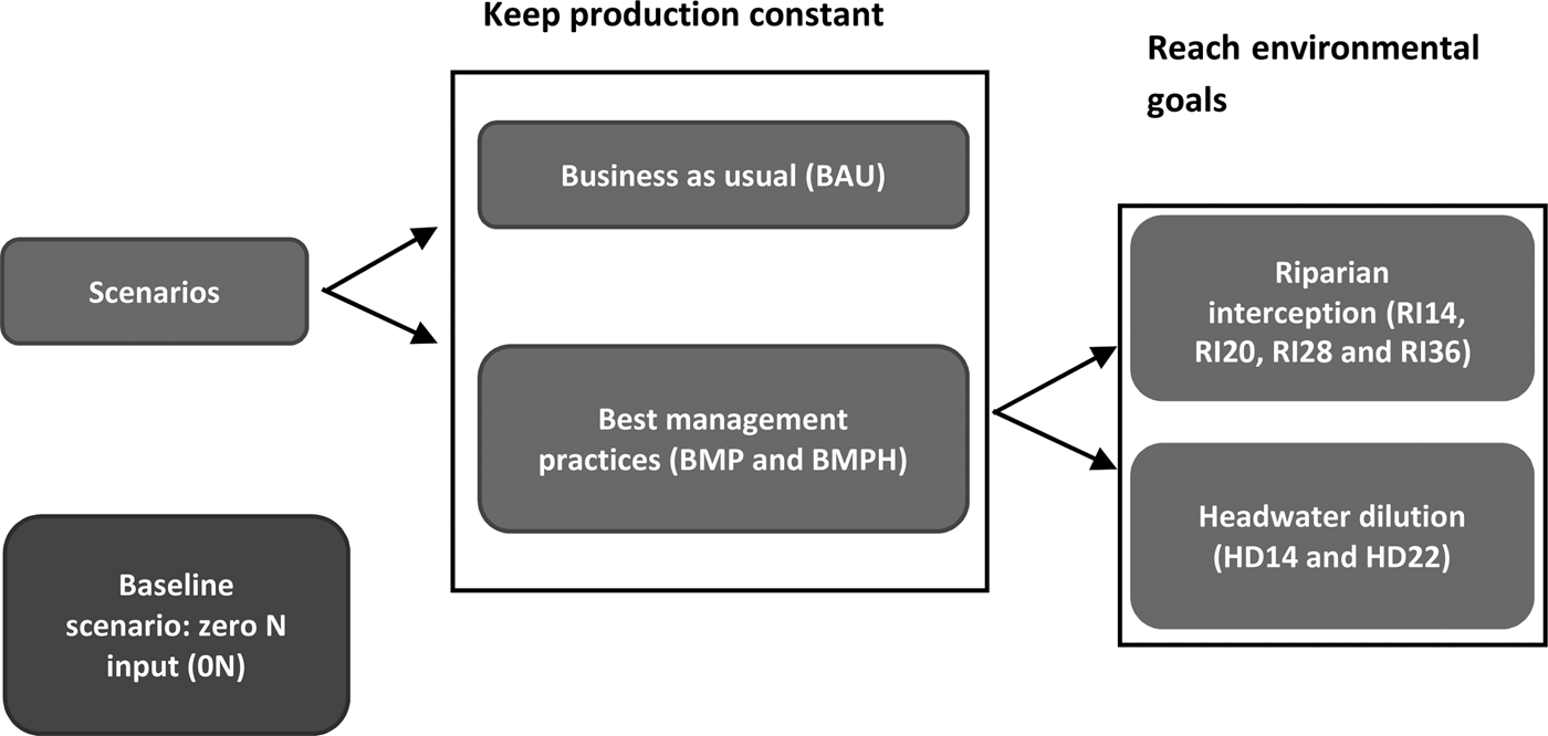
The scenarios were designed by researchers in collaboration with experts from technical institutes and agricultural cooperatives to investigate the different ways of mitigating negative effects on the nitrogen cascade from a heuristic perspective (i.e. regardless of their actual feasibility and without involvement of local stakeholders). The architecture of the scenarios (Fig. 1) shows the thrust and direction of the thinking adopted to create and classify the scenarios of the current study. The main objective was to assess the potential efficiency of landscape management actions as compared with field-scale mitigation measures (Schoumans et al., Reference Schoumans, Chardon, Bechmann, Gascuel-Odoux, Hofman, Kronvang, Litaor, Lo Porto, Newell and Rubaek2011).
Scenarios architecture within brackets the acronym used to name the scenarios. The scenario names (RI14/RI20/RI28/RI36 or HD14/HD22) indicate the proportion of area converted in environmental area (EA).

Data collection and ‘business as usual’ scenario
The catchment is being monitored for discharge, climate, stream and groundwater chemistry for more than two decades. The data used in the current paper are daily rainfall, air temperature, global radiation, Penman–Monteith potential evapotranspiration (PET), daily average discharge, grab-sampled nitrate concentration (sampling frequency varied between 1/day to 1/3 days during the period, with an average of 0.6/day). In the absence of climate data, the nearest weather station was used to fill the gaps. All details on the monitoring methods are available online (https://www6.inra.fr/ore_agrhys_eng/).
Farm surveys were performed in 2008 and 2013 to describe cropping systems (agricultural practices, land use and crop rotation) in the catchment as accurately as possible. Combined with field observations and remote-sensing data collected since 2002, these allowed reconstruction of the rotations and crop management practices for each field over 13 years (from 2002 to 2015). The Naizin–Kervidy catchment includes 268 fields corresponding to the smallest homogenous unit in terms of management practices. Management data included dates of plant sowing, tillage operations, manure and fertilizer applications (amount and type) and crop harvest. The main crops in the catchment are cereals (0.25 AA), maize (0.29), vegetables for industry (0.06), potato (0.06), oilseed rape (0.04) and grassland (0.25 as temporary grasslands, 0.05 as permanent on wet soils or slopes). Catch crops are planted according to NVZ regulations to avoid bare soils in intercropping periods. Livestock management, i.e. buildings and manure storage facilities, grazing management and animal feeding, was also described. Gaps and incoherencies in the surveys (especially regarding the grazing schedule) were dealt with by expert knowledge, mostly based on the practices of similar farms. For the 13-year period, farm management was considered as constant, i.e. certain changes such as owner changes, field exchange or changes in cropping systems were not taken into account. Agricultural data cannot be presented in more detail here because of confidentiality issues. Finally, the hedgerow network was included in the model, with 21 km in total (2013 data), corresponding to an average of 43 m/ha. This set of conditions is referred to as the ‘business as usual’ (BAU) scenario in the following sections.
Preserving scenarios
Two scenarios were built first, with the constraint of keeping overall agricultural production of the site almost constant. This was carried out in two steps (Fig. 1). In the first step, only field management was optimized towards best management practices (BMP scenario) and in the second step some landscape management was included. The new features of the Nitrates Directive programme adopted in 2014 were taken into account to design field management, though the regulations went into effect after the surveys. The main changes and checks of compliance with NVZ were:
– Modification of the fertilizer scheduling and manure application (longer period of ban). The application period depends on the crop, the type of effluent (manure, slurry, mineral) and the soil climate (e.g. on maize: solid manure could be applied from 15 January to 30 June according to the fourth Nitrate Directive and only until 15 May according to the fifth Nitrate Directive and for slurry from 15 February to 30 June then only from 1 April).
– Limited to 50 kg/ha of the Global Nitrogen Balance (GNB), i.e. an average soil balance at the farm scale over the last 3 years.
Though already mandatory since the fourth action programme in 2009, the fertilization balance for each crop was not strictly respected (according to references defined in the French implementation of the Nitrates Directive). This led to a 9% decrease of fertilizer inputs compared with the BAU scenario, concerning 0.26 of the catchment area. Likewise, catch crops were already sown systematically between winter and spring crops, as per the regulations; the current study simply simulated earlier sowing and delayed harvesting to increase their efficiency (e.g. for a potato–maize rotation the cover crop in the BAU scenario was sown on 25 September and harvested on 4 March whereas in the BMP scenario it was sown on 5 September (20 days earlier) and harvested on 25 March (20 days later)). The changes concerned 0.13 of the dates of catch crop sowing and 0.22 of the dates of catch crop harvest.
As imposed by regulation, the main stream network of the catchment is protected by narrow filter strips of vegetation (either grass or trees). It is possible, in theory, to plant more filtering structures by surrounding the fields with hedgerows. Therefore, crop management implemented in the BMP was completed by doubling the length of hedgerows (BMPH scenario). The locations of additional hedgerows were designed to optimize the mitigation of nitrogen fluxes, based on the studies of Kovar et al. (Reference Kovar, Kovarova, Bunce, Ineson and Brabec1996) and Benhamou et al. (Reference Benhamou, Salmon-Monviola, Durand, Grimaldi and Merot2013). The priority was to locate new hedgerows around fields with poorly drained soils, so that the tree roots can access shallow groundwater. They were also located around buildings, where farmers usually replant them as a priority, for aesthetic purposes. In such positions they can also potentially intercept NH3 emissions by buildings, but this effect is not yet simulated in the model used: only the effects on nitrate transfer will therefore be considered here. To double the hedgerow density as compared with the BAU scenario (i.e. 88 m/ha), additional hedgerows were positioned along roads and paths, this type of location being most easily accepted by farmers.
Transforming scenarios
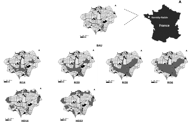
As described in Fig. 1, these two scenarios were constructed to further decrease nitrate losses, at the cost of reducing agricultural production. Previous work (Durand, Reference Durand2004; Durand et al., Reference Durand, Moreau, Salmon-Monviola, Ruiz, Vertes and Gascuel-Odoux2015) has shown that complying with Nitrate Directive regulations would probably not be enough to reach the standard of 11.4 mg N-NO3/l in stream water for a long time (at least two decades). For the two ‘landscape’ scenarios, the target is to comply with the Nitrate Directive standards by setting aside agricultural land according to different spatial patterns. Starting from the BMP scenario, the same agricultural area was set-aside and converted to ‘environmental area’ (EA) without any production objective (i.e. unfertilized grassland mown three times per year with exported biomass) but following two different strategies for location: (i) interception scenario, by placing the set-aside areas in riparian locations (RI scenario) to constitute wide riparian buffer strips and (ii) headwater scenario (HD scenario), by locating the set-aside grassland areas as a few large patches around the headwaters of streams. In the first case, the rationale is to add the possibility of maximizing retention of N-NO3 in the shallow pathways between fields and stream networks to the dilution effect of set-aside. In the second case, the rationale is to decrease N-NO3 concentrations in the upstream sections of the stream network, and also to maximize the contrast with the first scenario. Two options were tested for both scenarios, to reach about 0.15 and 0.20 of the catchment treated as an EA (Fig. 2). These proportions were determined from the extension of the classes of soil drainage regimes. In this catchment, about 0.05 of the soils are frequently waterlogged up to the soil surface and are not cultivated, 0.10 correspond to soils frequently waterlogged up to a depth of 40 cm, and 0.05 are temporarily waterlogged up to a depth of 40 cm (Curmi et al., Reference Curmi, Durand, Gascuel-Odoux, Mérot, Walter, Taha, Finke, Bouma and Hoosbeek1998). After examining the results and following a reviewer's advice, it was decided to further increase the size of the EAs in intercepting position. Therefore, scenarios with about 0.30 and 0.40 of EAs were also simulated. Since it was decided to preserve the field shapes in the implementation of these scenarios, the final proportions of EA varied slightly (Table 1). Therefore, six transforming scenarios were finally defined, named after the proportion of converted land use: HD14, HD22, RI14, RI20, RI28 and RI36.
Location of the converted grassland into the landscape management scenarios (light grey: agricultural area, black: buildings, hatched: natural areas, dark grey: environmental areas). BAU, business as usual; RI14, RI20, RI28, RI36, Riparian interception scenarios where 0.14, 0.20, 0.28 and 0.36 of the catchment are treated as an environmental area, respectively; HD14, HD22, headwater scenarios where 0.14 and 0.22 of the catchment are treated as an environmental area, respectively.

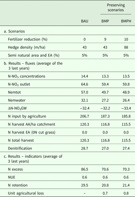
(a) Main features of the preserving scenarios for Naizin catchment (the units are specified in brackets) and (b) corresponding results

BAU, business as usual; BMP, best management practices; BMPH, best management practices with double hedgerows; EA, environmental area; N-NO3, nitrate nitrogen; Nemtot, total emission of reactive N to water bodies and atmosphere; Nemwater, nitrogen emission to water bodies; ΔN-NO3 GW, variation of N stored as NO3 in the groundwater; AA, agricultural area; NUE, nitrogen use efficiency.
All the values are in kg/ha/year of nitrogen (N) except for the concentration in mg/l of N-NO3 and dimensionless ratios.
Baseline scenario: zero nitrogen input
In this scenario, all the AAs were converted into unfertilized grassland, mown three times per year with exportation of biomass. The aim of this scenario (0N) was to simulate the dynamics of the quickest return to nearly pristine conditions. This type of land use was preferred over afforestation because preliminary modelling tests showed that it produced the lowest nitrate losses from soils in the short term.
Model
Presentation of the model
The model used is the agro-hydrological model Topography-based Nitrogen Transfers and Transformations (TNT2) fully detailed in Beaujouan et al. (Reference Beaujouan, Durand, Ruiz, Aurousseau and Cotteret2002). It is a distributed model running at a daily step time for multiple-year simulations, based on the main hypotheses of a TOPography based hydrological MODEL (TOPMODEL) for hydrological fluxes (Beven, Reference Beven1997) and on the crop model Simulateur mulTIdiscplinaire pour les Cultures Standard (STICS; Brisson et al., Reference Brisson, Gary, Justes, Roche, Mary, Ripoche, Zimmer, Sierra, Bertuzzi, Burger, Bussière, Cabidoche, Cellier, Debaeke, Gaudillère, Hénault, Maraux, Seguin and Sinoquet2003). The denitrification module has been described in Oehler et al. (Reference Oehler, Durand, Bordenave, Saadi and Salmon-Monviola2009), and the hedge module in Benhamou et al. (Reference Benhamou, Salmon-Monviola, Durand, Grimaldi and Merot2013). TNT2 has been designed to simulate water dynamics and nitrogen transfer and transformation for small, shallow aquifer catchments (typically <100 km2) (Beaujouan et al., Reference Beaujouan, Durand, Ruiz, Aurousseau and Cotteret2002). The model has been thoroughly tested and used for research and operational studies at catchment scale for about 15 years at about 20 different sites (Viaud et al., Reference Viaud, Durand, Merot, Sauboua and Saadi2005; Oehler et al., Reference Oehler, Durand, Bordenave, Saadi and Salmon-Monviola2009; Benhamou et al., Reference Benhamou, Salmon-Monviola, Durand, Grimaldi and Merot2013; Ferrant et al., Reference Ferrant, Durand, Justes, Probst and Sanchez-Perez2013; Durand et al., Reference Durand, Moreau, Salmon-Monviola, Ruiz, Vertes and Gascuel-Odoux2015). It is able to simulate non-agricultural areas as unmanaged grass or forest areas, hedges and housing and the interactions within the plant–soil–water continuum.
The catchment is represented by a regular square grid (25 × 25 m in the present application). Input data are climate variables (temperature, rainfall, PET, global radiation), the schedule of agriculture practices (date of sowing, harvesting, rotation, crop and catch crop management), fertilizer and manure type/amount applied, and pasture management. Output variables are obtained or aggregated at different spatial levels: pixel (regular square grid element), soils units (soil and hydrological variables), field (agriculture management) and the whole catchment (hydrological variables and total nitrogen loads) (Durand et al., Reference Durand, Moreau, Salmon-Monviola, Ruiz, Vertes and Gascuel-Odoux2015).
Simulation procedure
All scenarios were simulated with the latest version of the TNT2 model and parameter sets. In all cases, the model was first run for one hydrologic year (2002–2003) to ‘spin up’ (i.e. reach equilibrium from the initial state) the model. The calibration was done in two steps. Firstly, the hydrological part of the model was calibrated by maximizing the Nash–Sutcliffe (NS) coefficient (Nash and Sutcliffe, Reference Nash and Sutcliffe1970) for daily water discharge. As a starting point, the parameter values of the previous simulations (calibrated with a slightly different version of the model on a shorter period) were used. The two most sensitive parameters of the model (the transmissivity at soil saturation and its exponential decrease with depth, Beaujouan et al., Reference Beaujouan, Durand, Ruiz, Aurousseau and Cotteret2002; Moreau et al., Reference Moreau, Viaud, Parnaudeau, Salmon-Monviola and Durand2013) for the three soil types of the catchments (so six parameters in total) were adjusted using an iterative process. These were allowed to vary randomly within a 10% range around the initial value, then the best set was kept and a new 10% range of variation was defined. After ten iterations, the NS coefficient usually stabilized. Then, a trial-and-error approach was used to calibrate the nitrogen modules. A recommended set of parameters has been defined by the developers of the STICS model for most of the usual crops. Most soil parameters were set according to the detailed soil studies performed on this site (Curmi et al., Reference Curmi, Durand, Gascuel-Odoux, Mérot, Walter, Taha, Finke, Bouma and Hoosbeek1998; Tete et al., Reference Tete, Viaud and Walter2015; Viaud et al., Reference Viaud, Santillàn-Carvantes, Akkal-Corfini, Le Guillou, Prévost-Bouré, Ranjard and Menasseri-Aubry2018). The only parameters that were adjusted for the nitrogen processes were initial groundwater nitrate concentration, soil organic matter mineralization rates (Beff et al., Reference Beff, Morvan and Lambert2016) and denitrification rates. The calibration aimed at minimizing the relative mean error for nitrate concentrations and the error on cumulative N fluxes. The calibration was done on the period 2002–2005 for hydrology and the period 2002–2009 for nitrate. The comparison between outputs of the BAU scenario and observed data over the remaining simulation period (2005(8)–2015) were used to check the model's ability to simulate the functioning of the catchment. The same parameter set was used for the other scenarios, which were run for 10 years, after 2 years of BAU scenario, using the same climate data. The results of the scenarios are the mean values for the last 3 years of the simulation, to account for variations due to climate, to crop rotations and to the response time of the system.
Assessment indices
The scenarios were first compared using the changes in N fluxes at the catchment's outlet; however, this does not give a complete picture of the scenario performances, since changes may concern other N fluxes and stores, in particular N export in harvested crops and variations of denitrification or nitrification rates. All N transformation rates for the soil–plant–groundwater system have been calculated by the model. Variations in storage of soil organic matter, mineral N and groundwater N-NO3 have also been quantified. The main assessment indices were derived from the mass balance equations, as described below.
The following mass balance equation can be written thus (all variables expressed in kg N/ha/year, based on the total area of the catchment):
 $${\rm N\ input} = {\rm N\ output} + {\rm storage\ variations}$$
where N input is N total inputs in the catchment, N output is the N total outputs in the catchment and storage variations are N total variation of stores in soil, plant and groundwater compartments
 $${\rm N\ input} = {\rm NminF} + {\rm NorgF} + {\rm Ngraz} + {\rm Nfix} + {\rm Ndep}$$
where NminF is N input by mineral fertilizers, NorgF is N input by manure, Ngraz is N input from animal excretion during grazing, Nfix is N fixed by legumes (clover, grain legumes) and Ndep is N input by atmospheric deposition. In the following equations, Ndep is not included because it is assumed to be constant between scenarios and because its estimate is uncertain at this scale. Nitrogen input then corresponds to the total amount of N added on the fields by agriculture (spreading of manure, fertilizer application and N fixation).
 $${\rm N\ output} = {\rm Nharvest} + {\rm N}\hbox{-}{\rm N}{\rm O}_{\rm 3}{\rm outlet} + {\rm N}\hbox{-}{\rm N}{\rm H}_{\rm 3}{\rm em} + {\rm N}\hbox{-}{\rm N}_{\rm 2}{\rm Oem} + {\rm N}\hbox{-}{\rm N}_{\rm 2}{\rm em}$$
where Nharvest is N amount in the harvested parts of crops in AA (N harvest AA) and in the harvested parts of grass in EA (N harvest EA); N-NO3 outlet is the flux of nitrate in stream water at the outlet, N-NH3em is the N output by NH3 emission to the atmosphere, N-N2Oem is the N output by N2O emission to the atmosphere and N-N2em is the N output by N2 emission to the atmosphere.
The emission of ammonia resulting from mineral and organic fertilizer applications and from grazing are estimated by the model, but the emissions from livestock buildings within the catchment and the resulting short-range deposition of ammonia are not yet supported by the TNT2 model.
Since the model only simulates total denitrification, the N2O/N2 emission ratio is assumed to be constant and equal to 0.2 (N2O emission by nitrification not considered) (Drouet et al., Reference Drouet, Capian, Fiorelli, Blanfort, Capitaine, Duretz, Gabrielle, Martin, Lardy, Cellier and Soussana2011).
 $${\rm Storage\ variations} = \Delta {\rm Norgsoil} + \Delta {\rm Nplant} + \Delta {\rm N\ soil} + \Delta {\rm N}\hbox{-}{\rm N}{\rm O}_{\rm 3}{\rm GW}$$
where all these variables are calculated as the difference between the initial state and the final state for the last 3 years of simulation (negative if final <initial): ΔNorgsoil is the variation of N stored in organic form in the different compartments considered by the model (i.e. humus, undecomposed residues of plants or manure, biomass of microbial decomposers), ΔNplant is the variation of N amount of plants (including crops, grassland, trees…), ΔN soil is the variation of N sequestered in the soil and ΔN-NO3 GW is the variation of N stored as NO3 in the groundwater.
The groundwater seepage (i.e. deep flow not drained by the stream) is considered as insignificant in this catchment: ΔN-NO3 GW is then not an external flux but a storage variation due to the variation of groundwater volume (which tends to zero for long periods) and to the variation of nitrate concentration in the groundwater.
To assess the environmental and agronomic efficiency of the scenarios, the following indicators are proposed:
 $${\rm Nexcess} = {\rm Ninput} - {\rm Nharvest}$$
where Nexcess is the N agricultural surplus (i.e. the difference between Ninput and Nharvest)
 $${\rm NUE} = {\rm Nharvest}/{\rm Ninput}$$
where NUE is N use efficiency ratio (dimensionless).
The N use efficiency ratio may have different definitions (Shaviv and Mikkelsen, Reference Shaviv and Mikkelsen1993). In the current study, the NUE index is the ratio between the total N harvested and the total N input by agriculture computed at the catchment scale.
 $${\rm Nemwater} = {\rm N}\hbox{-}{\rm N}{\rm O}_{\rm 3}{\rm outlet} + {\rm} \Delta {\rm N}\hbox{-}{\rm N}{\rm O}_{\rm 3}{\rm GW}$$
where Nemwater is N emission to water bodies.
 $${\rm Nemtot} = {\rm Nemwater} + {\rm N}\hbox{-}{\rm N}{\rm H}_{\rm 3}{\rm em} + {\rm N}\hbox{-}{\rm N}_{\rm 2}0{\rm em}$$
where Nemtot is total emission of reactive N to water bodies and atmosphere.
 $${\rm Nret} = {\rm Nexcess} - {\rm Nemtot}$$
where Nret is the N ‘retention’ of all compartments (soil, atmosphere and plant).
Combining Eqn (9) with Eqns (1, 3, 4, 5, 7 and 8) leads to clarification of the meaning of Nret:
 $${\rm Nret} = {\rm N}\hbox{-}{\rm N}_{\rm 2}{\rm em} + \Delta {\rm Norgsoil} + \Delta {\rm Nplant} + \Delta {\rm N}\hbox{-}{\rm N}{\rm O}_{\rm 3}{\rm soil}$$
Thus, the common use of ‘retention’ was adopted by including N2 emissions by denitrification, which means that ‘retention’ represents the total amount of nitrogen not emitted as reactive N.
 $${\rm Unit\;\ agricultural\;\ loss} = {\rm \;} \displaystyle{{{\rm N\;\ harvest\;\ A}{\rm A}_{{\rm BAU}}-{\rm N\;\ harvest\;\ A}{\rm A}_{{\rm SC}}{\rm \;}} \over {{\rm N\;\ emwate}{\rm r}_{{\rm BAU}}-\; {\rm N\;\ emwate}{\rm r}_{{\rm SC}}}}$$
where unit agricultural loss is reduction of the harvested N amount between a given scenario and the BAU, standardized by the reduction of emission to water bodies (dimensionless).
Results
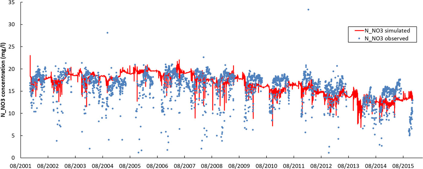
Many previous studies (Oehler et al., Reference Oehler, Durand, Bordenave, Saadi and Salmon-Monviola2009; Moreau et al., Reference Moreau, Ruiz, Raimbault, Vertes, Cordier, Gascuel-Odoux, Masson, Salmon-Monviola and Durand2012; Benhamou et al., Reference Benhamou, Salmon-Monviola, Durand, Grimaldi and Merot2013; Salmon-Monviola et al., Reference Salmon-Monviola, Moreau, Benhamou, Durand, Merot, Oehler and Gascuel-Odoux2013; Durand et al., Reference Durand, Moreau, Salmon-Monviola, Ruiz, Vertes and Gascuel-Odoux2015) have used the TNT2 model and shown its ability to simulate N cycling in various catchment studies. Some of these studies have been specifically performed on this catchment with a calibration focused on nitrate flows (Benhamou et al., Reference Benhamou, Salmon-Monviola, Durand, Grimaldi and Merot2013; Salmon-Monviola et al., Reference Salmon-Monviola, Moreau, Benhamou, Durand, Merot, Oehler and Gascuel-Odoux2013). Furthermore, a sensitivity analysis was carried out in 2013 (Moreau et al., Reference Moreau, Viaud, Parnaudeau, Salmon-Monviola and Durand2013). Thus, the detailed results of nitrate simulations are not developed in the current paper: the discharge at the outlet was simulated satisfactorily with NS of 0.74 and 0.81 for the calibration and verification period, respectively. For nitrate concentrations, the relative mean error (14%, no differences between calibration and verification period) was acceptable. It is always difficult to match simulated daily concentrations with observations resulting from daily grab sampling, but the general trends were adequately respected, both at the time event, seasonal and pluri-annual time steps (Fig. 3). For detailed discussion, see Ferrant et al. (Reference Ferrant, Oehler, Durand, Ruiz, Salmon-Monviola, Justes, Dugast, Probst, Probst and Sanchez-Perez2011) and Moreau et al. (Reference Moreau, Ruiz, Raimbault, Vertes, Cordier, Gascuel-Odoux, Masson, Salmon-Monviola and Durand2012). All observed data, especially discharge and nitrate concentration, are available online (http://www.agrhys.fr).
Daily nitrate (N-NO3) concentration observed (dot) and simulated (line) over 13 years. Colour online.

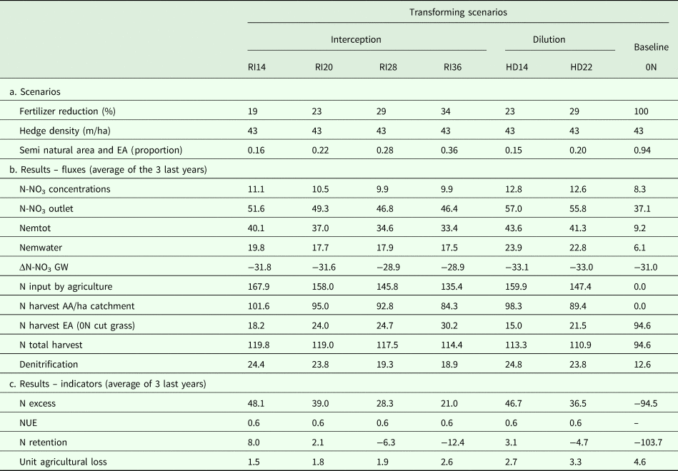
Tables 1 and 2 summarize the main results for the set of scenarios simulated.
(a) Main features of the transforming and baseline scenarios for Naizin catchment (the units are specified in brackets) and (b) corresponding results

RI14, RI20, RI28, RI36, Riparian interception scenarios where 0.14, 0.20, 0.28 and 0.36 of the catchment are treated as an environmental area, respectively; HD14, HD22, headwater scenarios where 0.14 and 0.22 of the catchment are treated as an environmental area, respectively; 0N, all agricultural areas converted into unfertilized grasslands; EA, environmental area; N-NO3, nitrate nitrogen; Nemtot, total emission of reactive N to water bodies and atmosphere; Nemwater, nitrogen emission to water bodies; ΔN-NO3 GW, variation of N stored as NO3 in the groundwater; AA, agricultural area; NUE, nitrogen use efficiency.
All the values are in kg/ha/year of nitrogen (N) except for the concentration in mg/l of N-NO3 and dimensionless ratios.
The results obtained from the BMPH scenario are very close to the BMP scenario, suggesting that in this context, the densification of the hedgerow network does not reduce nitrate transfer significantly.
While all the mitigation scenarios produced a decrease of nitrate fluxes and concentrations, the BMP and dilution scenarios (HD14 and HD22) did not reach the Nitrate Directive standard of 11.4 N-NO3 mg/l. Implementation of the BMP guidelines reduced fertilization by 9%, producing only a small decrease of mean concentration from 15.2 to 14.1 N-NO3 mg/l, while implementation of the dilution scenarios produced a larger decrease in fertilizer inputs (23 and 29%). By contrast, all the interception scenarios resulted in a final nitrate concentration below the ND standard. Therefore, the reduction of nitrate concentration allowed by the set-aside measure depended not only on the environmental zone areas but also on the location of these zones. To examine the mechanisms responsible for the higher efficiency of interception scenarios, it is necessary to explore the results further, using the indices defined above (Figs. 4–8).
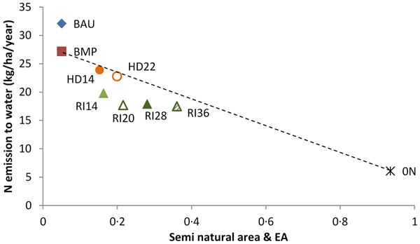
Emissions to water v. area of environmental area and semi-natural area. BAU, business as usual; BMP, best management practices; RI14, RI20, RI28, RI36, Riparian interception scenarios where 0.14, 0.20, 0.28 and 0.36 of the catchment are treated as an environmental area, respectively; HD14, HD22, headwater scenarios where 0.14 and 0.22 of the catchment are treated as an environmental area, respectively; EA, environmental areas. Colour online.

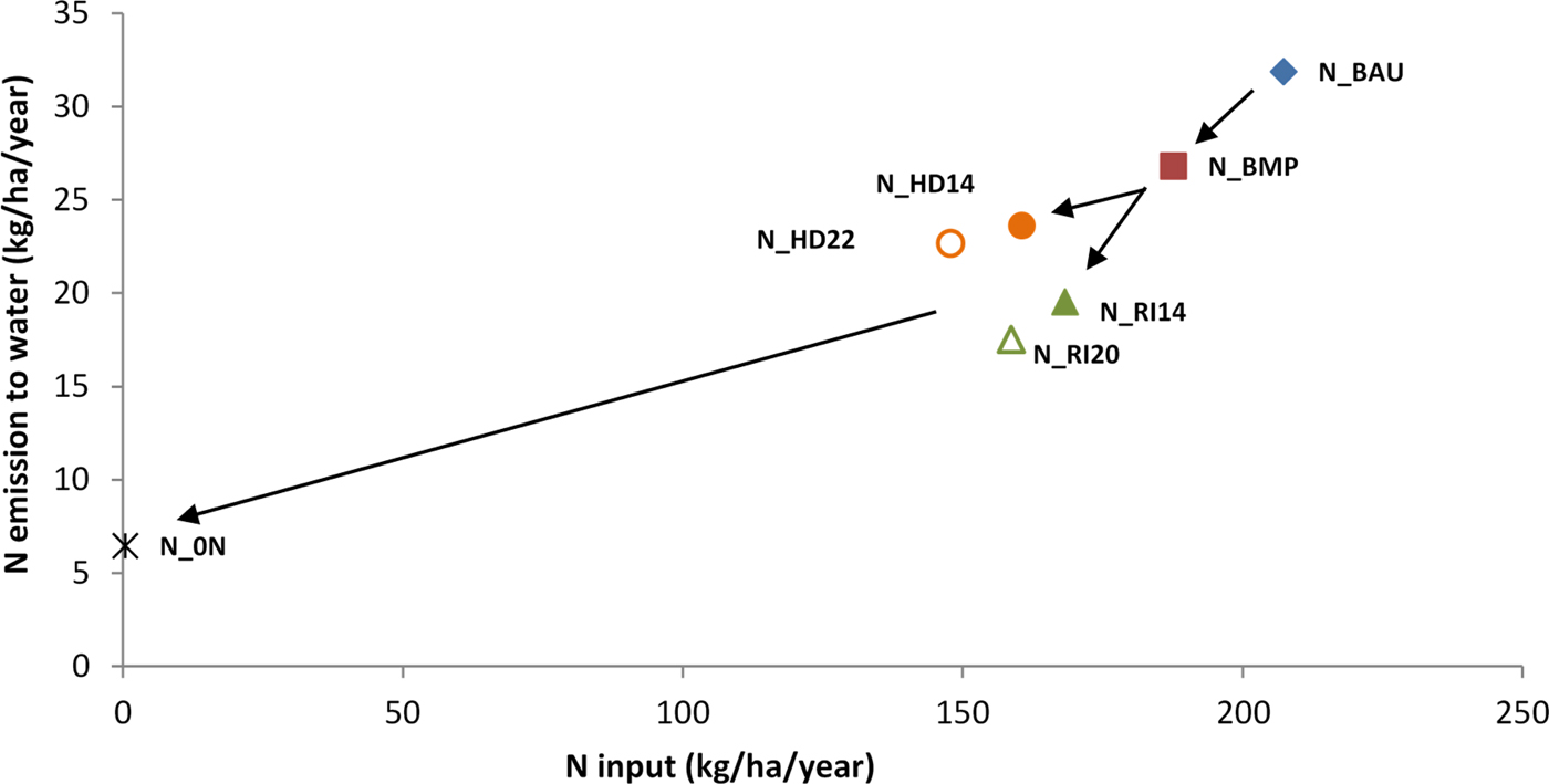
Emissions to water v. nitrogen (N) input. The arrows schematize the implementation of the different measures from the current state (business as usual N_BAU) to the most restrictive scenario (zero nitrogen input) passing by best management practices (BMP) and set-aside areas. RI14, RI20, RI28, RI36, Riparian interception scenarios where 0.14, 0.20, 0.28 and 0.36 of the catchment are treated as an environmental area, respectively; HD14, HD22, headwater scenarios where 0.14 and 0.22 of the catchment are treated as an environmental area, respectively. Colour online.

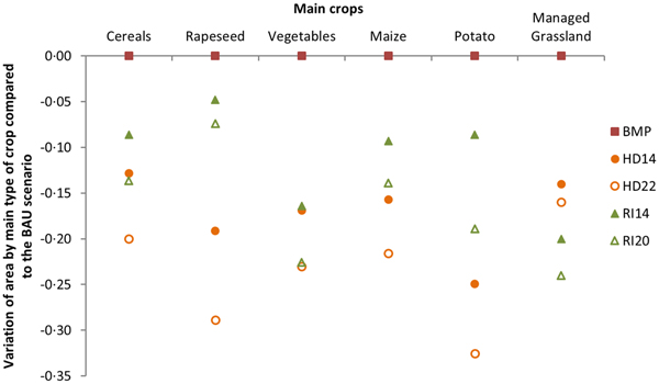
The variation of agricultural area use for the main crops in all scenarios compared with business as usual (BAU) scenario. BMP, best management practices; RI14, RI20, Riparian interception scenarios where 0.14 and 0.20 of the catchment are treated as an environmental area, respectively; HD14, HD22, headwater scenarios where 0.14 and 0.22 of the catchment are treated as an environmental area, respectively. Colour online.

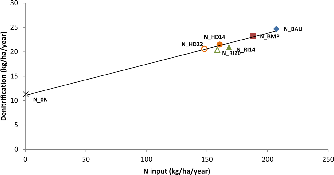
Denitrification load v. nitrogen (N) total agricultural input. BAU, business as usual; BMP, best management practices; RI14, RI20, RI28, RI36, Riparian interception scenarios where 0.14, 0.20, 0.28 and 0.36 of the catchment are treated as an environmental area, respectively; HD14, HD22, headwater scenarios where 0.14 and 0.22 of the catchment are treated as an environmental area, respectively; 0N, all agricultural areas converted into unfertilized grasslands. Colour online.

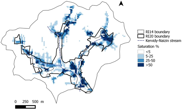
Map of soil saturation with water (% of simulation time when the water table reached at least the deeper soil layer). RI14, RI20, Riparian interception scenarios where 0.14 and 0.20 of the catchment are treated as an environmental area, respectively Colour online.

Relationship between the area of environmental zones and the nitrate losses to water
Figure 4 shows that the N emissions to water were proportional to the amount of non-agricultural areas (environmental zones + semi-natural areas) in this catchment when considering the BMP, HD and baseline_0N scenarios only. The RI scenarios were under this line, showing an enhanced retention of nitrogen due to the interception processes. However, the distance to the line decreases when the set-aside area increases beyond 0.20, showing that the benefit of interception is highest when the set-aside zones are the closest to the stream.
It is worth noting that after 10 years with no agricultural input (0N scenario), nitrate losses (N-NO3outlet) were still as high as 36 kg N/ha/year and nitrate concentration was still 8.9 mg N-NO3/l.
Relationship between nitrate emissions in water and nitrogen input
The different mitigation measures led to a decrease in total N input at catchment scale, directly by reducing fertilization and excess stocking rates at grazing (BMP), and indirectly by reducing AA and N fixation (no legumes in set-aside grassland). This decrease of NO3 emissions to water appeared to be strongly, but not linearly, correlated to the decrease of input (Fig. 5).
Figure 5 shows that, for the same area converted, the reduction of fertilizer input is higher for dilution (HD14 and HD22) compared with interception scenarios (RI14 and RI20), e.g. reduction of 23% for HD14 v. 19% for RI14. This difference is due to the initial land use of areas converted into EA: for the interception scenario it is predominantly grassland areas, which in the Naizin–Kervidy catchment are generally less fertilized than the arable crop areas. This is illustrated by Fig. 6, showing that for the same conversion rate, the dilution scenarios (HD14 and HD22) systematically impact the annual crops area more than the interception scenarios (RI14 and RI20), with the exception of the vegetable area that is similarly reduced in both types of landscape scenarios. The potato area showed the largest decline in HD22 scenario with a reduction of 33%.
Therefore, it can be concluded that the higher efficiency of the interception scenarios is not due to larger reduction of N input.
Denitrification fluxes according to the location of environment areas
Figure 7 shows that denitrification was highly correlated with total agricultural input of N. The N emissions by denitrification were more than halved between the BAU and 0N scenarios, from 25 to 11 kg N/ha/year. This figure also shows that, for the same set-aside area, denitrification was slightly lower in the interception scenarios than in the dilution scenarios, although N input was higher. This suggests that denitrification is not simply related to the waterlogging conditions that were more frequent downslope than upslope (Fig. 8).
Therefore, it can be concluded that the higher efficiency of the interception scenarios in reducing nitrate losses is not due to enhanced denitrification. The results also suggest that this higher efficiency for nitrate did not result in pollution swapping towards N2O emissions.
Relationship between the harvested nitrogen and the environmental area
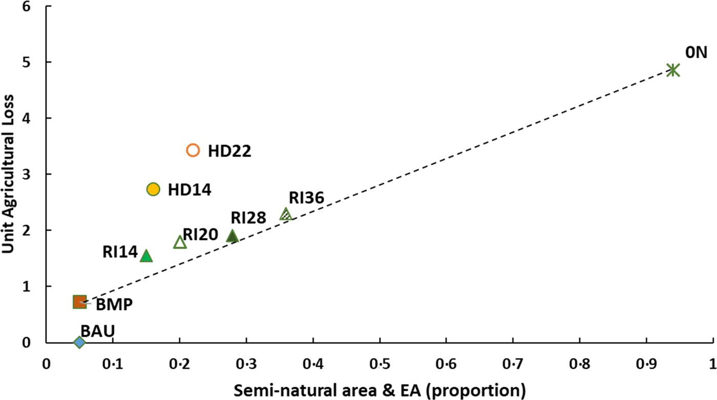
To assess the best combination of mitigation measures, i.e. high reduction of N losses combined with low reductions in agricultural products, the agricultural loss index was calculated as the ratio between the loss in agricultural production at catchment scale and the corresponding decrease in nitrate emissions to water (Eqn 11). Plotting this index v. the proportion of EA shows that the BMP, interception and 0N scenarios are on the same line, while the dilution scenarios are above this line (Fig. 9). This highlights that the dilution scenarios reduced proportionally more the uptake of N by the crops than the losses of nitrate.
Unit agricultural loss v. proportion of semi-natural and environmental areas (EA). BAU, business as usual; BMP, best management practices; RI14, RI20, RI28, RI36, Riparian interception scenarios where 0.14, 0.20, 0.28 and 0.36 of the catchment are treated as an environmental area, respectively; HD14, HD22, headwater scenarios where 0.14 and 0.22 of the catchment are treated as an environmental area, respectively; 0N, all agricultural areas converted into unfertilized grasslands. Colour online.

The total N harvested is 19% lower in the baseline 0N (1.00 AA as unfertilized cut grass) compared with crops of BMP scenario (1.00 AA as crops or grassland). When considering this total N harvested, the difference between HD and RI scenarios is even more visible: in the RI scenario, N harvested in the EAs compensated almost entirely for the loss of N harvest due to set-aside, whereas in the HD scenario the total N harvest lost is around 10 kg/ha compared with the BAU scenario (Tables 1 and 2).
This suggests that the higher efficiency of interception scenarios is mostly due to sustained uptake by the vegetation in spite of decreasing N input, and to the lower land use change (managed grassland replaced by unfertilized cut grassland for 0.20 AA for RI14 and 0.24 for RI20) compared with dilution scenarios, where the higher reduction of rapeseed, potato and wheat areas (Fig. 7) resulted in a decrease in N uptake by crops. Using this unit loss index shows more clearly that the RI14 scenario is the most efficient of the transforming scenarios tested: the index is minimum for this scenario, meaning that for a further extension of the set-aside area, the harvested N decreased more rapidly than the N emissions.
Discussion
The set-aside scenarios simulated in the current study were built to explore their ability to mitigate N losses, in particular nitrate, in addition to the tuning of management practices. The impact of implementing the Nitrate Directive in vulnerable areas (Barnes et al., Reference Barnes, Willock, Hall and Toma2009; Worrall et al., Reference Worrall, Spencer and Burt2009; Velthof et al., Reference Velthof, Lesschen, Webb, Pietrzak, Miatkowski, Pinto, Kros and Oenema2014) and optimizing agricultural practices at the field scale (mainly by more balanced fertilization, good management of grazed grassland and the introduction of catch crops) (Oenema et al., Reference Oenema, Witzke, Klimont, Lesschen and Velthof2009; Buckley and Carney, Reference Buckley and Carney2013) is well documented, showing significant, yet limited, efficiency. It is therefore important to combine changes in agricultural management and landscape levers (buffering capacity of wet areas and hedges, dilution by reducing cropped and fertilized area). Using a model allows simulation of scenarios at the catchment scale over several years and comparison of contrasting strategies of mitigation. Any modelling exercise is undermined by uncertainties linked to simplifications in process representation and imperfect data. Their impact on the conclusions are limited in the current study by (i) the amount and quality of data accumulated in this catchment for many years and (ii) focusing interpretation on the comparison between scenarios rather than absolute values of predicted variables.
In the current study area, strict implementation of the Nitrate Directive does not allow acceptable levels of nitrogen emissions to be achieved, in the mid-term, due to the intensive agricultural context and the legacy of nitrogen in soils and groundwater. In a context where agricultural production is dominated by arable crops and land use is very constrained, the current study shows that application of BMP results in only small reductions in nitrate losses (2–5%), as well as agricultural production, and increases NUE of the system slightly.
The legacy of N in this catchment has two origins. First, it is due to changes in soil organic matter, both in terms of content and quality, which resulted from the conversion of permanent grassland to arable land in the late 1960s, and from the massive addition of livestock slurry and manure since then (Canevet, Reference Canevet1992; Houot et al., Reference Houot, Pons, Pradel and Tibi2016). Second, it is due to the continuous increase of N concentrations in shallow groundwater (now well over 30 mg/l N-NO3), constituting a store whose depletion delays the effects of agricultural changes on stream water (Molénat et al., Reference Molénat, Durand, Gascuel-Odoux, Davy and Gruau2002, Reference Molénat, Gascuel-Odoux, Aquilina and Ruiz2013; Durand et al., Reference Durand, Moreau, Salmon-Monviola, Ruiz, Vertes and Gascuel-Odoux2015). This depletion occurs in all scenarios, even BAU, because of enforcement of the Nitrate Directive in the last 15 years. In the baseline 0N scenario, after 10 years the groundwater depletion still accounts for 0.85 of the emissions to water, showing that the steady state between N losses and land use is far from being reached. However, for the last 3 years of simulation, the depletion rate of nitrate concentration in groundwater is comparable between scenarios, which allows their comparison. Longer simulations were not possible, because the TNT2 model requires detailed agricultural data for each field over the whole period, and they were available for 10 years only. Simulation data were obtained from farm surveys and, although carefully carried out, some data are missing or have been poorly documented, particularly concerning pasture management; expert knowledge was necessary to fill the gaps. Moreover, surveys did not reveal outliers such as significant over-fertilizing: this may be due to strict compliance with regulations or to farmers ‘smoothing’ their declared practices according to the regulation. In the second case, this would mean that the optimized scenarios (BMP and BMPH) would be more efficient compared with the simulated BAU scenario. Another reason for the modest effect of this scenario is that the changes were limited: strict adherence to the Nitrate Directive does not imply real fertilization equilibrium or great efficiency of catch crops, difficult to achieve in commercial farm conditions (Edwards-Jones, Reference Edwards-Jones1993; Wallace and Moss, Reference Wallace and Moss2002).
The results of previous studies by Benhamou et al. (Reference Benhamou, Salmon-Monviola, Durand, Grimaldi and Merot2013) and Durand et al. (Reference Durand, Moreau, Salmon-Monviola, Ruiz, Vertes and Gascuel-Odoux2015) corroborate the hedge scenario (BMPH) results obtained in the current study. Doubling the hedgerow density is not enough to observe significant results in terms of reduction in nitrate losses. The main reasons are, first, that nitrate is transferred mainly by sub-surface flow, which is hardly intercepted, if at all, by hedges, and second, that the area covered by hedges is not significant to produce a dilution effect. Locating the hedges preferentially on poorly drained soils (where sub-surface flux is the shallowest) was not sufficient to enhance their efficiency significantly. The effect of hedgerows on ammonia emission scavenging is not taken into account here, and may be significant in terms of atmospheric pollution, but it is unlikely that it is large enough to affect nitrate losses. On the contrary, enhancing the deposition of ammonia might result in a pollution swapping effect detrimental to water quality.
The main results of the current study were that the decrease in N-NO3 emissions produced by set-aside scenarios is not proportional to the area converted into EA and that the location of EA is decisive to maximize the reduction of nitrogen emissions. There are two reasons for this: first, the landscape changes impact the crop area and type of crops differently, depending on location. As observed in most small catchments in Brittany, intensive cropping systems (cereals, maize, grain legumes and potatoes with high N inputs and limited soil cover during winter) are located mainly on deep, well-drained soils, while grassland occupies slopes and bottom locations. This is even more true in the current study area because it is classed as a NVZ, and riparian vegetation buffers had been planted all along the stream network. Incidentally, this measure does not appear to be sufficient to reach the Nitrate Directive targets, as already stated by Haag and Kaupenjohann (Reference Haag and Kaupenjohann2001).
The consequence is that the interception scenarios had a lower effect on N input and crop production than dilution effects. Despite this, the interception scenarios were more efficient at reducing nitrogen emissions to water, so extension of the riparian buffer zones by a minimum of 10% of the catchment area makes it possible to reach satisfactory levels of pollution in this context, by combining a dilution effect and the interception of nitrate leached uphill. Apparently, this interception is due mainly to retention in soils and to plant uptake, because denitrification is about the same in the RI and HD scenarios. This effect on denitrification is consistent with previous studies in Brittany context (Moreau et al., Reference Moreau, Ruiz, Raimbault, Vertes, Cordier, Gascuel-Odoux, Masson, Salmon-Monviola and Durand2012; Durand et al., Reference Durand, Moreau, Salmon-Monviola, Ruiz, Vertes and Gascuel-Odoux2015). Clément et al. (Reference Clément, Pinay and Marmonier2002) and Oehler et al. (Reference Oehler, Durand, Bordenave, Saadi and Salmon-Monviola2009) have already observed that denitrification rates in the riparian zones of the region are controlled tightly by nitrate availability. It is likely that removing the direct spreading of nitrogen decreases the overall denitrification of the riparian zone. When increasing the set-aside area beyond 0.20 of the catchment area, the enhanced retention tends to diminish (RI28 and RI36 scenarios). The likely reasons for that are twofold:
(1) The amount of nitrate coming from shallow groundwater to the soil decreases upslope, because the groundwater level is on average deeper, and reaches the soil profile less frequently (this effect is both predicted by the model and observed in the lysimeter transects monitored in the catchment (Molénat et al., Reference Molénat, Gascuel-Odoux, Davy and Durand2005).
(2) Grassland production in this area is often limited by water availability during the second half of summer, but less limited downslope than upslope, again because of the water supply by shallow groundwater to the soil. Therefore, N uptake potential by the grassland areas may decrease when this supply decreases.
The second reason for better efficiency of the interception scenarios is that these scenarios affect the land use of the riparian area, where the mean residence time of water is the shortest (Molénat et al., Reference Molénat, Durand, Gascuel-Odoux, Davy and Gruau2002). Therefore, the short- or mid-term effects on stream water concentrations are likely to occur much faster than for the dilution scenarios, which affect uphill areas with a much longer residence time. Indeed, at the end of the simulation, average concentrations in groundwater in the two sets of scenarios are similar, but in the interception scenarios the lowest concentrations are located downhill v. uphill in the dilution scenarios, with less direct contribution to stream water. It follows that extending the scenario simulations for two decades would show a progressive decrease of the differences between the two options, even if the interception scenarios would probably remain more efficient.
Finally, in this catchment, the RI14 scenario appears to be the best compromise, because it achieved the ND target for stream water relatively quickly, without impacting agricultural production too much at the catchment level. Still, these results must be taken with caution and cannot be easily generalized. First, they are limited to catchments with similar hydrological settings, i.e. dominated by the dynamics of shallow groundwater exchanging with soil water in the lower parts of the hillslopes. Second, it is clear that the optimal extension of the interception zone will depend on the dynamics of the waterlogged area, which is very site-specific, depending on local topography, i.e. a regionalized modelling scheme would be necessary to obtain a more robust estimate. Third, there are always large uncertainties in denitrification modelling, especially at the catchment scale, particularly because of the very high variability of hydromorphic soil properties (Durand et al., Reference Durand, Moreau, Salmon-Monviola, Ruiz, Vertes and Gascuel-Odoux2015); and finally, the physiology of plants under waterlogged conditions probably remains poorly simulated, even if this issue is relatively limited since the waterlogging conditions do not persist during the growing season in the major part of the set-aside zone.
Of course, in the real world, the impact of this type of measure on individual farms would vary widely, making it socially difficult to implement, even in the hypothesis of compensation for the loss of income. However, Brittany, like many other agricultural regions in Europe, has a large proportion of farmers ceasing activity for age or economic reasons (0.30 of the farms have changed ownership in the last decade). Such results could be used to orientate pre-emption of land by local authorities to set-aside parts of the properties that are changing hands. Beforehand, these results should be consolidated by applications in different contexts.
Conclusion
In intensive agriculture areas with a large legacy of nitrogen in soils and groundwater, the application of mandatory BMP in the fields is often not sufficient to reach acceptable nitrogen concentrations in streams in the short term. Mixing agricultural land use with unmanaged areas may be a way forward, if the location of the converted areas maximizes the retention efficiency and minimizes the impact on agriculture production. The current study shows the ability of distributed modelling to help find this optimal location. It confirms interest in poorly drained lowlands, which combine lower agronomic potential and high retention efficiency, and suggests that, in this particular case, setting aside 0.10–0.15 of the catchment area would be a good compromise between environmental objectives and most limited impacts on agriculture production. These results differ from most studies on the effects of riparian areas on nitrate losses because (1) they suggest that enhanced denitrification is not the major process responsible for the higher efficiency of the interception scenarios and (2) they explore the effects of a wide range of scenarios, in terms of location and size of the set-aside areas.
These conclusions are of course specific to this type of hydrological setting and climate and subjected to large uncertainties, given the simplified representation of reality given by the model. Assessing the effect on gaseous emissions and deposition of ammonia and indirect N2O emissions should be the next step for a more complete assessment of these scenarios. More generally, these types of land use management are also potentially beneficial for the mitigation of other pollutants and for preservation of biodiversity. This suggests that such policy should be submitted to a multicriteria evaluation, in terms of ecosystem services and economic impacts.
Acknowledgements
The authors are very grateful to all the staff of the Agrhys Observatory, especially to S. Busnot, Y. Hamon, M. Faucheux and N. Gillet (field work), G. Le Henaff (databases) and P. Pichelin (GIS).
Financial support
This work was funded by the French National Research Agency (ESCAPADE project in AGROBIOSPHERE program, ANR-12-AGRO-0003). The farm surveys were performed within the MOSAIC project of the AGROBIOSPHERE program, ANR-12-AGRO-0005. The grant of the first author was co-funded by Arvalis.
Conflict of interest
None.
Ethical standards
Not applicable