Introduction

Projections have suggested that global warming will disproportionately affect polar regions (e.g. Reference HoughtonHoughton and others, 2001; Reference Holland and BitzHolland and Bitz, 2003); consequently the behavior of Arctic (and high-latitude) glaciers may be among the first clear indicators of the onset and severity of climate change. Some recent observations and analyses of glacier behavior (e.g. Reference Arendt, Echelmeyer, Harrison, Lingle and ValentineArendt and others, 2002; Reference Meier, Dyurgerov and McCabeMeier and others, 2003; Reference OerlemansOerlemans, 2005) support this conclusion. Other studies, however, point to a lack of coherent regional trends or otherwise suggest that the behavior of some Arctic glaciers with respect to enhanced greenhouse warming is equivocal (Reference DowdeswellDowdeswell and others, 1997; Reference Dyurgerov and MeierDyurgerov and Meier, 2000; Reference SerrezeSerreze and others, 2000; Reference AbdalatiAbdalati and others, 2004). To reduce this apparent ambiguity, therefore, improvements in the observational database are needed, specifically increases in both the number and geographic distribution of those glaciers being monitored (Reference Dyurgerov and MeierDyurgerov and Meier, 2000), and in understanding how glacier behavior may lag climatic forcings (e.g. Reference OerlemansOerlemans and others, 1998; Reference OerlemansOerlemans, 2005). Because of the latter, however, glaciers within a particular geographic area do not always show a consistent pattern of advance and retreat. Such non-synchronous response to climate change is exemplified by the behaviors of Rabots Glaciär and Storglaciären, two small valley glaciers in the Swedish Arctic (Equation (1)). The purpose of this paper is to present the results of numerical modeling that indicate this non-synchronous behavior is due, in large part, to differences in individual glacier dynamics, and ultimately in their response times.

Fig. 1.

Location of Storglaciären and Rabots Glaciär. Note the similarity in size of the glaciers. Dotted lines on the glaciers show the approximate positions of the velocity profiles shown in Figure 3.

Fig. 2.

Measured and/or estimated changes in ice volume and terminus position of Storglaciären and Rabots Glaciär. Data for volume changes on Storglaciren are from Reference HolmlundHolmlund (1987, Reference Holmlund1988) and updated using recent mass-balance measurements. Volume changes are estimated prior to 1946. Volume changes for Rabots Glaciär (shown with uncertainties) are estimated largely from measured changes in ice surface elevations or those depicted in maps (see Reference Brugger, Refsnider and WhitehillBrugger and others, 2005). All other data are from unpublished reports of the Tarfala Research Station and Reference BruggerBrugger (1992). (After Reference Brugger, Refsnider and WhitehillBrugger and others, 2005.)

Recent Behavior of the Glaciers

Changes in glacier length and ice volume for Rabots Glaciär and Storglaciären were compared by Reference Brugger, Refsnider and WhitehillBrugger and others (2005) and are summarized in Figure 2. Both glaciers advanced late in the 19th century and then retreated in response to a warming of ~1˚C at the beginning of the 20th century (Reference HolmlundHolmlund, 1987, Reference Holmlund1993; Holmlund and Jansson, 1999). The terminus position and geometry of Storglaciären more-or-less stabilized in the mid-1980s, by which time ice volume had decreased by about 131×106^m3. Subsequently the glacier experienced a slight increase in volume without any significant change in terminus position. These post-1980 volume increases may be due to contemporaneous increases in (winter) precipitation and the development of a more maritime climatic regime in the region (Reference DowdeswellDowdeswell and others, 1997; Reference Pohjola and RogersPohjola and Rogers, 1997). The reaction of Rabots Glaciär in response to the same warming lagged behind that of Storglaciären, and its initial rates of retreat were low (~2ma^–1). Retreat generally increased to >11ma^–1 by 1959 and has remained relatively constant thereafter. By the mid-1980s, concomitant reductions in the volume of Rabots Glaciär (~135×106^m3) were comparable to those of Storglaciären, but more noteworthy is the fact that since then the glacier has lost an additional 20×106^m3 of ice. Thus as noted by Reference HolmlundHolmlund (1988, Reference Holmlund1993) and Reference BruggerBrugger (1997), it appears that Storglaciären is, or was, in quasi-equilibrium, at least with respect to mass/volume changes, while Rabots Glaciär continues to adjust to the earlier climatic warming.

Glacier Characteristics and Mass Balances

Longitudinal profiles based on their 1980 geometries and surface velocities of Storglaciären and Rabots Glaciär are contrasted in Figure 3a and b. Mean ice thickness (~100 and 85m respectively), maximum thickness (250 and 175 m), and thickness variations are all greater for Storglaciären, resulting in distinctly different variations of horizontal velocities. This is perhaps the first hint that these two glaciers should behave rather differently. Hypsometries of the glaciers (Fig. 3c) are similar.

Fig. 3.

(a, b) Longitudinal thickness and velocity profiles for (a) Storglaciären (see Reference Hooke, Calla, Holmlund, Nilsson and StroevenHooke and others, 1989) and (b) Rabots Glaciär (Reference BruggerBrugger, 1992). Thickness profiles are based on 1980 glacier geometries, and velocities were measured in the mid-1980s. Approximate positions of the velocity profiles are shown in Figure 1. All vertical scales and horizontal scales are the same. (c) Individual glacier hypsometry and average mass balance for the interval 1981– 2003. (Data from unpublished reports of the Tarfala Research Station.) Net-balance gradients are based on linear regressions.

The consistent increases of summer over annual velocities on Rabots Glaciär seen in Figure 3b are attributed to meltwater production that facilitates basal sliding (Reference BruggerBrugger, 1992). More pertinent for the present study, however, is the close similarity of the winter and annual velocity profiles. The assumption made here, as it has been elsewhere (e.g. Reference MacGregor, Riihimaki and AndersonMacGregor and others, 2005), is that basal sliding is minimal during the winter, so the contribution of sliding to annual velocities is negligible. Measured seasonal variations of surface velocities on Storglaciären (Reference Hooke, Calla, Holmlund, Nilsson and StroevenHooke and others, 1989; R.LeB. Hooke, unpublished data) suggest that sliding might account for 5–10% of annual velocities. Moreover, Reference HansonHanson (1995) and Reference Albrecht, Jansson and BlatterAlbrecht and others (2000) found that little or no sliding was required to fit modeled surface velocities to those observed on Storglaciären.

Very few meteorological or climatological data are available for the valley of Rabots Glaciär, making it difficult to directly compare the respective microclimates under which each glacier exists. Alternatively, specific net mass-balance curves (Fig. 3c) might be compared, as these essentially capture the meteorological parameters (temperature, precipitation, radiation balances and so forth) relevant to glacier regime. Using the method of Reference KuhnKuhn (1984), Reference BruggerBrugger (1992) showed that the specific net-balance curves for each glacier are generally similar in form from year to year (see also Reference RasmussenRasmussen, 2004). It is obvious (Fig. 3c) that mass-balance gradients (db/dz, where b is specific net mass balance and z is altitude) differ between the glaciers. The steeper gradient on Storglaciären (~0.008mw.e.m^–1) indicates a greater mass turnover, and therefore perhaps also hints at its quicker response time and greater climatic sensitivity (Reference OerlemansOerlemans, 2005). In contrast, db/dz on Rabots Glaciär (~0.005mw.e.m^–1) suggests a slower response time.

Interannual variations in the net mass balance of the glaciers are well correlated (r ² = 0.78, n = 23, p < 0.0001). Thus one might expect the climatic ‘events’ that forced the retreat of the glacier from their ~1910 maximums were synchronous; in other words, the glaciers reacted to a regional climate signal. This is corroborated by historical evidence (photographs, unpublished reports, etc.) that indicates both glaciers began retreating at the same time. Because of local filtering of that regional signal (by interactions between/among topography and local energy and mass balances), it could be argued that each glacier experienced climate change of different magnitude. Regressions between net mass balance and temperature (e.g. Reference BruggerBrugger, 1992; Reference Holmlund, Karlén and GruddHolmlund and others, 1996) suggest, however, that the climatic forcing induced by the warming was comparable for both glaciers, being on the order of –0.3 to –0.4mw.e. a^–1. The underlying assumption is that no strong feedback occurs between changes in glacier geometry (particularly surface elevation) and mass balance (cf. Reference Harrison, Elsberg, Echelmeyer and KrimmelHarrison and others, 2001).

Glacier geometry and mass balance allow first-order estimates of response time τ to be calculated in several ways. Reference Jόhannesson, Raymond, Waddington and OerlemansJόhannesson and others (1989a) presented a simple geometric argument that suggests

where is a thickness scale (variously taken as mean ice thickness, maximum ice thickness or some other measure) and b ₀(l ₀) is the mass balance at the terminus that characterizes the glacier’s datum, or equilibrium state (subscript ‘0’). However, in light of potential difficulties in assigning precise datum-state values of and b ₀(l ₀) for both Storglaciären and Rabots Glaciär, a simplified formulation of the form

is used (Reference OerlemansOerlemans, 2001, Reference Oerlemans2005), where β is the mass-balance gradient, db/dz, s is the surface slope and L is the glacier length. Here τ _L is a ‘length response time’ (Reference OerlemansOerlemans, 2001). As noted previously, it is reasonable to assume the mass-balance gradients are relatively constant, and furthermore that the 1910 geometries of each glacier reflected some quasi-equilibrium. Thus for Storglaciären and Rabots Glaciär, respectively, representative values for β ₀ are ~0.008 and 0.005 mw.e.m^–1, s ₀ ~ 0.130 and 0.115, and L ₀ ~ 4065 and 4610m yield estimates of τ _L of ~60 and 105 years. Despite the generality of Equation (2), these results imply a significantly longer (length) response time for Rabots Glaciär.

The Model

A one-dimensional, time-dependent flow model was used to estimate the response times of the glacier to small perturbations in mass balance. The model, discussed in detail by Reference BindschadlerBindschadler (1982), is a finite-difference approximation to the continuity equation

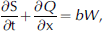
where Q is the volume flux through a glacier cross-section of area S, t is time, x is the center-line distance, b is the specific net balance and W is glacier width. Net mass balance is subsequently assumed to consist of a steady- or datum-state value b ₀ upon which is superimposed a perturbation b ₁. Glacier width and cross-sectional area are parameterized as a function of ice thickness H along x using the empirical relations

and

The constants D, E and F as well as values for H and W were determined from existing topographic maps and radio-echo soundings. Volume flux is related to the center-line surface velocity U _s through use of a flux shape factor f ^* that yields a velocity averaged over S, hence

Surface velocity is

where A and n (=3) are flow-law parameters, f is a shape factor used to account for drag imparted by valley walls (Reference NyeNye, 1965), ρ is the density of ice (=900 kgm^–3), g is gravitational acceleration (=9.8ms^–2) and α is the slope of the ice surface. In the model, surface slopes were longitudinally averaged over distances substantially greater than ice thicknesses. Equation (7) ignores basal sliding, but, as discussed above, sliding is not thought to be important in the long-term mean velocities of either glacier. However, this is a point that is returned to in a subsequent section of this paper.

The finite-difference implementation together with specified boundary conditions uses an iterative predictor– corrector technique to approximate the true solution to Equations (3–7) within some defined level of accuracy (expressed in terms of maximum allowable changes between iterations). Only the lower reach of each glacier could be accurately modeled because of both the complications arising from the confluence of tributaries, and, in the case of Rabots Glaciär, sparse velocity and mass-balance data for the tributaries. Thus a constant-head boundary condition (Reference BindschadlerBindschadler, 1980, Reference Bindschadler1982; Reference Bindschadler and RasmussenBindschadler and Rasmussen, 1983; Reference BruggerBrugger, 1997) was imposed such that

the volume flux is

where A _uo is the surface area in the datum state up-glacier from the modeled reach. While this boundary condition preserves mass continuity, it does not capture the time-dependent behavior of the unmodeled sections of the glaciers. Instead it implies that these regions of the glaciers respond instantaneously to mass-balance perturbations, whereas in reality changes in geometry upstream of the boundary would result in changes in volume flux that would propagate more slowly through each glacier. Consequently, to minimize the influence of this boundary condition on glacier behavior, small mass-balance perturbations were used so that glacier geometry (i.e. H and α) remains relatively constant in this region and thus the volume flux imposed is comparable to that which would be given by Equation (6). Nevertheless, the potential effects of this boundary condition are evaluated below.

Datum states for the glaciers were defined by their mid-1980s geometries, as these correspond to a time when detailed measurements of the surface velocity field and mass balance of Rabots Glaciär were carried out (Reference BruggerBrugger, 1992). Values for f were tuned in accordance with measured surface velocities (Fig. 3a and b). Because of this tuning, modeling results are not sensitive to the choice of the flow-law parameter A. Once tuned, a set of b ₀(x) for each glacier was found that would maintain these geometries, and the model was then run (with b ₁(x) = 0) to insure a steady-state configuration. For that reason, minor adjustments in initial glacier geometry occur, but differences between actual and modeled datum-state ice thicknesses did not exceed 0.5 m except at the termini where they were on the order of 5 m. It bears mentioning that the values of b ₀(x) required to maintain datum-state geometry of Storglaciären were in most cases comparable to the values shown in Figure 3c, again suggesting that the glacier is close to being in equilibrium with existing climate. b ₀(x) values required to preserve the mid-1980s geometry of Rabots Glaciär were generally 0.5–0.75mw.e. a^–1 more positive than those shown in Figure 3c, except close to the terminus where they are ~1.25mw.e. a^–1 more positive. It must be emphasized that the particular datum-state glacier geometry, mass-balance parameters and tuning criteria were selected in order to determine the response times of the glaciers. No attempt is made here to either simulate historic variation in glacier length (and volume) or predict future behavior in response to ongoing climate warming.

Response Times Deduced from Numerical Modeling

Steady-state mass balances were uniformly (b ₁ 6≠ f (z)) altered using step-like perturbations of –0.01, –0.03 and –0.05mw.e. a^–1, and the model was allowed to run until new steady-state profiles were established. In practice, steady state was achieved when changes in ice thickness between successive iterations were <1%. Results of the modeling experiments are summarized in Table 1. Figure 4 shows examples of the temporal evolution of glacier geometry in response to such perturbations (in this case, b ₁ = 0.05 mw.e. a^–1) and the corresponding changes in terminus position. These examples are representative of all modeling runs, but also show that even for the largest b ₁ used the change in ice thicknesses at the head boundary is small for Storglaciären (~2%) and slightly larger for Rabots Glaciär (~10%). From Figure 4 it can be seen that the new equilibrium profile of Storglaciren is established more quickly that that for Rabots Glaciär. However, the time periods required to achieve new steady state (varying between ~200 and 500 years) are, to some extent, an artifact of the modeling and reflect the termination of the approach to equilibrium specified by desired level of accuracy. These numbers are therefore less significant for the present discussion.

Table 1.

Model-derived volume timescales calculated for three mass-balance perturbations

Fig. 4.

An example of the temporal evolution of the new steady-state profiles for (a) Storglaciären and (b) Rabots Glaciär in response to a step-like perturbation in mass balance b ₁ (here b ₁ = –0.05mw.e. a^–1). Intermediate profiles are shown at 50 year intervals. All vertical scales and horizontal scales are the same. Insets show details of the terminus retreat.

What is more significant is that a characteristic response time for each glacier can be estimated from modeled changes in volume. Expressed in terms of a volume timescale τ _v (Reference Jόhannesson, Raymond and WaddingtonJόhannesson and others, 1989b), the response time is

where V ₁(1) is the change in ice volume in the glacier’s final steady state (t = 1) and A ₀ is the total area of the glacier in its datum state. Although thickness changes at the model boundaries are relatively small (Equation (4)), they do imply volume changes up-glacier, which might be especially significant for Rabots Glaciär. Volume timescales calculated directly from Equation (9) using only volume changes over the model reaches are therefore minimum estimates. Mean values for τ _v for Storglaciären and Rabots Glaciär (Table 1) are 106±10 and 154±6 years respectively.

Obviously, more realistic estimates of each glacier’s volume timescale need to account for volume loss in the areas up-glacier of the head boundaries that could not be modeled. These quantities were thus estimated by first extrapolating final thickness changes in the model reaches into the unmodeled regions. Excluding the large changes that occur near the termini, these vary linearly with distance (r ² > 0.98). When multiplied by the (unmodeled) area affected by these changes and added to modeled volume losses, better approximations of V ₁(1) are obtained (Table 1). This procedure tends, however, to overestimate volume losses in the unmodeled regions for two principal reasons. Firstly it ignores the small reductions in surface area that would be expected there. Secondly, in the regions of tributary confluence, the effective cross-sectional area (defined as being perpendicular to flow) is wider than it is down-valley. Decreased ice flux could therefore be accommodated by smaller decreases in ice thickness. If instead decreased flux were wholly accommodated by decreases in velocity, no decreases in thickness would occur. Using these estimates of additional volume loss thus yields approximate upper limits to the calculated response times.

Not surprisingly, volume losses in the unmodeled area calculated in this manner are significantly larger for Rabots Glaciär and increase total volume loss by 30–47%. For Storglaciären, increases in total volume loss are more modest, ranging from about 17% to 20%. Concomitant increases in each glacier’s response time are given in Table 1. The modeling thus suggests that the volume timescale of Storglaciären to step-like perturbations in mass balance is on the order of 120–140 years. Rabots Glaciär, on the other hand, is characterized by a longer response time of τ210–230 years. The difference in the glaciers’ volume timescales using these estimates is substantially greater than that determined when changes in volume up-glacier of the head boundary are ignored (these being about 90 and 50 years respectively). This suggests that the effect of including the latter increases the calculated difference between τ _v for Storglaciären and Rabots Glaciär. Because of the aforementioned uncertainties involving the boundary condition, it is the relative magnitudes of τ _v that are deemed important here rather than the actual values. As a measure of response, then, the volume timescale for Rabots Glaciär is at least ~1.5 times that of Storglaciären, and perhaps as much as ~1.7 times greater.

Discussion and Conclusions

It should be stressed that the volume timescales determined in this study are derived from a relatively simple model simulating a hypothetical and highly idealized climate-change scenario. Nevertheless, it is worthwhile to briefly consider the significance of τ _v estimated here with the observed recent behavior of Storglaciären in particular, since measurements of it are more abundant and detailed. As noted previously, it has been suggested that Storglaciären is in quasi-equilibrium with existing climate (Reference HolmlundHolmlund, 1988, Reference Holmlund1993; Reference BruggerBrugger, 1992, 1997). If it is also taken to be true that the glacier was in or near steady state at the 1910 maximum then its response time, defined by Reference NyeNye (1960) as the time required for glacier geometry to be within 1 – (1/e) of its final steady-state value, is estimated to be τ45 years (= 0:63× (1980 – 1910); Reference HolmlundHolmlund, 1988). Fitting the measured (or estimated, as opposed to modeled) time variations of volume V ₁(t) (Reference HolmlundHolmlund, 1988) to

(Reference Jόhannesson, Raymond and WaddingtonJόhannesson and others 1989b) might also yield estimates of the glacier’s volume timescale. Again under the assumption that Storglaciären is now in steady state and V ₁(1) ~ 1.31× 108^m3, τ _v is ~33 years (Equation (5)). If it is assumed based on the foregoing discussion that τ _v is ~45 years, then V ₁(1) is ~1.57× 108^m3. Allowing both τ _v and V ₁(1) to be free parameters, a best fit to Equation (10) is obtained with V ₁(1) ~ 1.89× 10⁸m3 and τ _v ~ 63 years. For comparison, requiring τ _v to be ~127 years as suggested by the modeling results, V ₁(1) would be ~3.02×108m3. Although all the fitted curves shown in Figure 5 are statistically significant (r ² > 0.92), none appear to fit the observations very well.

Fig. 5.

Observed or estimated variations in ice volume for Storglaciären fitted to an equation of the form V ₁(t) = V ₁(1)× 1 e (t/τ ^v) . The different curves correspond to different assumptions made regarding the value of V ₁(1) or τ _v given in the explanation; curves are labeled according to estimated parameters (see text for discussion).

There are a number of factors that are likely to be contributing to the discrepancy between these estimates of τ _v and that based on the modeling in this study (and others made for Storglaciären (e.g. Reference Raper, Briffa and WigleyRaper and others, 1996; Reference HookeHooke, 2005, p. 381)), the simplicity of the model notwithstanding. These include:

1. 1. Climatic change early in the 20th century was only approximately step-like, and subsequent variations have occurred. Thus the glacier’s behavior undoubtedly reflects a more complex forcing (cf. Reference Raper, Briffa and WigleyRaper and others, 1996).

2. 2. That Storglaciren was in equilibrium around 1910 is questionable (Reference StroevenStroeven, 1996), therefore introducing the potential for yet more complexity in its response. In particular, Reference Brugger, Refsnider and WhitehillBrugger and others (2005) speculated that had Storglaciren not fully completed its response to the climate change driving its Little Ice Age advance, (a) the onset of retreat would have been delayed, and (b) the actual magnitude of post-1910 retreat and reductions in volume would be less than what might be expected. In effect, this would reduce both V ₁(1) and the apparent time to complete its response to the ~1˚C warming during the early 20th century.

3. 3. The mass-balance perturbation associated with this warming was probably not small (Reference HookeHooke, 2005). As stated previously, this perturbation was probably about –0.4mw.e. a^–1, nearly an order of magnitude larger than the largest used in the modeling experiments. This is significant because Equation (9) strictly holds for small perturbations only (Jόähannesson and others, 1989b), so volume timescales derived from observed volume changes, driven by such a large forcing, might not be compatible with those determined from the modeling in the present study.

4. 4. The characteristic response time (or volume timescale) of Storglaciären in its 1910 configuration may have been shorter than in its present state. Reference Bahr, Pfeffer, Sassolas and MeierBahr and others (1998) showed that τ _v might decrease with increasing glacier size (or volume; Reference Raper, Briffa and WigleyRaper and others, 1996) precisely because larger glaciers extend to lower elevations where their termini experience greater rates of ablation. For the specific case of Storglaciären, the steep bed slope combined with the mass-balance gradient could result in a substantially larger value for b ₀(l ₀) at its 1910 terminus and therefore a shorter τ _v via Equation (1). In particular, assuming again that db/dz is constant, a terminus elevation of 1050m and an equilibrium-line altitude of ~1400m (very roughly corresponding to a steady-state mass balance for the glacier’s 1910 geometry), b ₀ (l ₀) would have been on the order of 2.8mw.e. a^–1. Thus an estimate of τ _v for the glacier in 1910 is . Regardless of the thickness scale used, as a first approximation it is reasonable to expect that varies proportionally to mean ice thickness, so that is Since b ₀(l ₀) is ~1.0 for the interval 1981– 2003, the glacier’s current response time would also be , more than double that for 1910. In the modeling, where a specific net-balance curve is used that will maintain Storglaciären’s mid-1980s geometry, b ₀(l ₀) is ~0.75mw.e. a^–1 so that τ _v is The foregoing analysis, however crude, might reconcile the longer response deduced from the modeling with that suggested by the observed behavior. It furthermore underscores the importance of the bed slope near the terminus in the glacier’s response to climate change (presumably through local dynamics of flow), as has been noted elsewhere (e.g. Reference Rasmussen and ConwayRasmussen and Conway, 2001).

5. 5. It was mentioned earlier that during recent decades this region of the Arctic seems to be experiencing more winter precipitation, which may mean Storglaciären’s approach to its current ‘steady state’ was hastened, or that the observed quasi-equilibrium is in fact transient.

6. 6. Finally the model’s failure to incorporate sliding could also explain, to some extent, the resultant longer volume timescale compared with those based on its observed changes in geometry. Reference BruggerBrugger (1992) considered the effects of sliding in an admittedly ad hoc manner by modifying f ^* in Equation (4), and these results are included in Table 1. In the model, sliding is invariant along x, so the values of τ _v shown are probably not quantitatively correct. However, these results do show qualitatively that (1) by virtue of increased mass turnover, sliding shortened the volume timescales as would be expected; (2) the values of τ _v determined for both Storglaciären and Rabots Glaciär in this study are robust even if sliding contributes ~10% to mean annual surface velocity; and (3) the magnitude of sliding required to reconcile τ _v inferred from the model with that based on observed volume changes on Storglaciären would need to be substantial (~50% or more), and hence arguably not reasonable.

In conclusion, numerical modeling indicates that in their mid-1980s configurations and for small mass-balance perturbations the volume timescale of Rabots Glaciär is ~215 years while that of nearby Storglaciären is ~125 years. In view of the vagaries of ‘real-world’ climate signals and actual as opposed to perceived steady states, it is difficult to assess whether these response times can, at present, be verified by observations of the glaciers’ respective behaviors. Moreover, the glaciers’ response time may not have been constant through time. By virtue of a rather steep bed slope, the advanced and thin terminus of Storglaciären in 1910 extended to a much lower elevation and hence was subjected to substantially greater ablation. Storglaciären would have therefore been particularly sensitive to the reduced ice flux brought about by climate warming, and this is reflected in the shorter response time estimated for its 1910 geometry. The same cannot be said for Rabots Glaciär, because of its relatively flat bed slope. Thus the difference in response times of the two glaciers may have been even greater in the past. However, what is emphasized here is not a particular individual response time, but their relative magnitudes. A longer response time explains why Rabots Glaciär lagged behind Storglaciären in its initial reaction to the warming that occurred early in the 20th century, and why significant ice retreat and mass loss continues today. When considering their response to CO₂-induced global warming, Storglaciären might be expected to react before Rabots Glaciär, and any response by Rabots Glaciär could be superimposed on its final adjustments to the earlier warming.