1 Introduction
Gas flows in microporous media are involved in many important applications. For example, nano-scale pores are dominant in ultra-tight shales, leading to high Knudsen number (Kn) even though the gas is dense (Darabi et al. Reference Darabi, Ettehad, Javadpour and Sepehrnoori2012). On the other hand, the high in situ pressure and temperature in deep-seated shales make the non-ideal gas effect non-negligible (Ma et al. Reference Ma, Sanchez, Wu, Couples and Jiang2014; Wu, Chen & Li Reference Wu, Chen and Li2015; Wang, Guo & Wang Reference Wang, Guo and Wang2016). Another important application of high Kn non-ideal gas flow is carbon dioxide burying and storage (White et al. Reference White2005; Vishal et al. Reference Vishal, Ranjith, Pradhan and Singh2013). Actually, carbon dioxide may exhibit more significant coupling because of its stronger non-ideality than methane (Wang, Lan & Li Reference Wang, Lan and Li2008). In addition, high Kn non-ideal gas flow also exists in some nanofluidics, which has attracted attention recently (Wang & Li Reference Wang and Li2003; Wang et al. Reference Wang, Lan and Li2008; Wu et al. Reference Wu, Liu, Reese and Zhang2016). Physically, the high Kn effect causes gas slippage at a fluid–solid interface, or even breaks the continuum assumption (Xu & Li Reference Xu and Li2004), while the non-ideal gas effect results in failure of the equation of state of an ideal gas, and in changing of transport properties (e.g. dynamic viscosity).
Predictions of gas flow behaviours in micro/nanoporous media with both high Kn and non-ideal gas effects are required. However, classical theories for high Kn porous flow are mostly based on the ideal gas model (Klinkenberg Reference Klinkenberg1941; de Socio & Marino Reference de Socio and Marino2006), while the theories concerning real gases generally neglect the high Kn effect (Al-Hussainy, Ramey & Crawford Reference Al-Hussainy, Ramey and Crawford1966). Recently, researchers have started to study the coupling of high Kn and non-ideal gas effects using pseudo-pressure methods (Villazon et al. Reference Villazon, German, Sigal, Civan and Devegowda2011), volume averaging methods (Lasseux et al. Reference Lasseux, Valdes Parada, Ochoa Tapia and Goyeau2014), pore-work modelling (Ma et al. Reference Ma, Sanchez, Wu, Couples and Jiang2014) and multiscale simulation (Wang et al. Reference Wang, Guo and Wang2016). However, there are still many debates and some results are even contradictory. For example, Wu et al. (Reference Wu, Chen and Li2015) found that the non-ideal gas effect promotes high Kn gas flow, while Ren et al. (Reference Ren, Guo, Guo and Wang2015) discovered that the non-ideal gas effect restrains the flow. The reason is that, in each work, a specific gas at given pressure and temperature is studied, thus the conclusions hold only for the corresponding conditions. When the temperature and pressure range is extended, Ma et al. (Reference Ma, Sanchez, Wu, Couples and Jiang2014) found that the coupling of high Kn and non-ideal gas effects may have different results. However, the coupling mechanism remains unclear and a quantitative analysis is lacking.
Because of the limited understanding in the coupling mechanism of high Kn and non-ideal gas effects, most models for engineering practices mainly consider the high Kn effect, while neglecting the non-ideal gas effect (Darabi et al. Reference Darabi, Ettehad, Javadpour and Sepehrnoori2012) or using simplified approximations (Lunati & Lee Reference Lunati and Lee2014). In the measurement of rock samples, some gas properties (e.g. the dynamic viscosity and compressibility factor) are usually assumed constant when calculating the gas permeability (Rushing et al. Reference Rushing, Newsham, Lasswell, Cox and Blasingame2004; Gensterblum, Ghanizadeh & Krooss Reference Gensterblum, Ghanizadeh and Krooss2014). This approach may cause biases due to the variation of gas properties from upstream to downstream. A clear description of the mechanism in high Kn non-ideal gas flow is helpful to interpret the measured data more accurately.
In this work, high Kn non-ideal gas flow is investigated through theoretical analysis and numerical simulation. The coupling of high Kn and non-ideal gas effects is quantitatively divided into four types, based on which effect is dominant and whether the non-ideal gas effect promotes or restrains the flow. Using multiscale numerical simulations, all four types are demonstrated and the results agree well with theoretical predictions. Based on the analysis, we propose a more precise model to calculate gas permeability from measurements, which better bridges the laboratory experiment and the reservoir engineering.
2 Theoretical analysis
For most gas flows in micro/nanoporous media, the velocity is small enough that the flow is laminar. We further assume the flow is isothermal and along the main direction of the permeability tensor. In addition, we focus on steady-state flow in this work, which is a basic flow type in reservoir studies (Ahmed & McKinney Reference Ahmed and McKinney2005). The steady-state assumption has been commonly used for measuring rock properties in laboratory experiments.
For high Kn flow in a porous medium, the traditional theory of Darcy is no longer valid. Klinkenberg (Reference Klinkenberg1941) introduced the pressure-dependent permeability into Darcy’s law, which is widely used and has been physically explained in recent studies (Civan Reference Civan2010; Darabi et al. Reference Darabi, Ettehad, Javadpour and Sepehrnoori2012; Lasseux et al. Reference Lasseux, Valdes Parada, Ochoa Tapia and Goyeau2014; Wu et al. Reference Wu, Ho, Germanou, Gu, Liu, Xu and Zhang2017):
 $$\begin{eqnarray}Q_{m}=\unicode[STIX]{x1D70C}(p)\frac{K(p)}{\unicode[STIX]{x1D707}(p)}\left(-\frac{\text{d}p}{\text{d}x}\right)=\frac{K(p)}{\unicode[STIX]{x1D708}(p)}\left(-\frac{\text{d}p}{\text{d}x}\right),\end{eqnarray}$$
where
 $\unicode[STIX]{x1D70C}$
is the gas density,
 $p$
the gas pressure,
 $K$
the apparent permeability,
 $\unicode[STIX]{x1D707}$
the gas dynamic viscosity and
 $\unicode[STIX]{x1D708}$
the gas kinematic viscosity. These properties are dependent on pressure.
After separating variables in (2.1) and integrating from upstream to downstream, we have
 $$\begin{eqnarray}\int _{0}^{L}Q_{m}\,\text{d}x=-\int _{p_{1}}^{p_{2}}\frac{K(p)}{\unicode[STIX]{x1D708}(p)}\,\text{d}p.\end{eqnarray}$$
For a steady state, the mass flux is constant:
 $$\begin{eqnarray}Q_{m}=\frac{1}{L}\int _{p_{2}}^{p_{1}}\frac{K(p)}{\unicode[STIX]{x1D708}(p)}\,\text{d}p.\end{eqnarray}$$
The linear relationship between apparent permeability
 $K$
and Knudsen number Kn is adopted (Klinkenberg Reference Klinkenberg1941)
 $$\begin{eqnarray}K=K_{0}(1+bKn),\end{eqnarray}$$
where
 $K_{0}$
is the intrinsic permeability and
 $b$
is the Kn-based slip factor. Comparing to the model proposed by Beskok & Karniadakis (Reference Beskok and Karniadakis1999), the linear relationship is generally valid in the slip and early transition regime (Kn up to 0.5) with a maximum error of 7 %. The Knudsen number is defined as (Knudsen Reference Knudsen1933)
 $$\begin{eqnarray}Kn=\unicode[STIX]{x1D706}/l,\end{eqnarray}$$
where
 $\unicode[STIX]{x1D706}$
is the mean free path of gas molecules and
 $l$
the characteristic length of the flow. The hard sphere model is adopted to calculate the mean free path of real gases (Bird Reference Bird1983):
 $$\begin{eqnarray}\unicode[STIX]{x1D706}=\frac{\unicode[STIX]{x1D707}}{\unicode[STIX]{x1D70C}}\sqrt{\frac{\unicode[STIX]{x03C0}}{2R_{g}T}}=\unicode[STIX]{x1D708}\sqrt{\frac{\unicode[STIX]{x03C0}}{2R_{g}T}},\end{eqnarray}$$
where
 $R_{g}$
is the specific gas constant and
 $T$
is the temperature. Combining (2.4)–(2.6), we have
 $$\begin{eqnarray}K(p)=K_{0}\left[1+\frac{b}{l}\unicode[STIX]{x1D708}(p)\sqrt{\frac{\unicode[STIX]{x03C0}}{2R_{g}T}}\right].\end{eqnarray}$$
Substituting (2.7) into (2.3) and assuming
 $l$
is constant, the mass flux is
 $$\begin{eqnarray}Q_{m}=\frac{K_{0}}{L}\int _{p_{2}}^{p_{1}}\frac{1}{\unicode[STIX]{x1D708}(p)}\,\text{d}p+\frac{K_{0}(p_{1}-p_{2})}{L}\frac{b}{l}\sqrt{\frac{\unicode[STIX]{x03C0}}{2R_{g}T}}.\end{eqnarray}$$
Through (2.8), the mass flux is calculated by the intrinsic permeability
 $K_{0}$
, the kinematic viscosity
 $\unicode[STIX]{x1D708}$
and the ratio
 $b/l$
. To replace the integral term in (2.8), we introduce the harmonic mean of the kinematic viscosity between
 $p_{1}$
and
 $p_{2}$
:
 $$\begin{eqnarray}\unicode[STIX]{x1D708}_{char}=\frac{p_{1}-p_{2}}{\displaystyle \int _{p_{2}}^{p_{1}}\frac{1}{\unicode[STIX]{x1D708}(p)}\,\text{d}p}.\end{eqnarray}$$
For gases, since the kinematic viscosity decreases monotonically with pressure, a unique pressure
 $p_{char}$
exists, at which the kinematic viscosity equals the harmonic mean, i.e.
 $\unicode[STIX]{x1D708}(p_{char})=\unicode[STIX]{x1D708}_{char}$
. Later, we will prove that the complex non-ideal gas behaviours can be characterized by
 $p_{char}$
and
 $\unicode[STIX]{x1D708}(p_{char})$
, i.e. the mass flux is identical once the gases have identical
 $p_{char}$
and
 $\unicode[STIX]{x1D708}(p_{char})$
. Thus, we define
 $p_{char}$
as the characteristic pressure and
 $\unicode[STIX]{x1D708}(p_{char})$
as the characteristic viscosity of a real gas.
Substituting (2.9) into (2.8):
 $$\begin{eqnarray}Q_{m}=\frac{p_{1}-p_{2}}{L}K_{0}\left[\frac{1}{\unicode[STIX]{x1D708}(p_{char})}+\frac{b}{l}\sqrt{\frac{\unicode[STIX]{x03C0}}{2R_{g}T}}\right].\end{eqnarray}$$
Equation (2.10) can be further simplified by introducing the apparent permeability at the characteristic pressure,
 $K(p_{char})$
, which is obtained by substituting
 $p_{char}$
into (2.7):
 $$\begin{eqnarray}K(p_{char})=K_{0}\left[1+\frac{b}{l}\unicode[STIX]{x1D708}(p_{char})\sqrt{\frac{\unicode[STIX]{x03C0}}{2R_{g}T}}\right].\end{eqnarray}$$
Combining (2.10) and (2.11), we finally have
 $$\begin{eqnarray}Q_{m}=\frac{K(p_{char})}{\unicode[STIX]{x1D708}(p_{char})}\frac{p_{1}-p_{2}}{L}.\end{eqnarray}$$
Equation (2.12) offers a concise expression to calculate mass flux for high Kn non-ideal gas flow. In (2.12), the characteristic viscosity is calculated by (2.9) using the real gas kinematic viscosity data. The characteristic pressure is therefore determined by the relationship between viscosity and pressure. In this work, the real gas density and viscosity data are from the National Institute of Standard and Technology (NIST) in the United States.
Equation (2.12) correlates the gas mass flux with the apparent permeability at the characteristic pressure. In the laboratory, by substituting the measured mass flux into (2.12), the apparent permeability at the characteristic pressure can be determined. In reservoir engineering, the steady-state mass flux can be calculated using the permeability data obtained in the laboratory. After introducing the characteristic pressure and viscosity, the mass flux expression (2.12) has the same form as the classical Darcy’s law for an incompressible fluid. Equation (2.12) can also recover the expression for an ideal gas, for which the equation of state is
 $p=\unicode[STIX]{x1D70C}^{id}R_{g}T$
and the dynamic viscosity is pressure independent (Smits & Dussauge Reference Smits and Dussauge2006). The kinematic viscosity of ideal gas is
 $$\begin{eqnarray}\unicode[STIX]{x1D708}^{id}(p)=\frac{\unicode[STIX]{x1D707}^{id}}{\unicode[STIX]{x1D70C}^{id}}=\frac{\unicode[STIX]{x1D707}^{id}R_{g}T}{p}.\end{eqnarray}$$
Here
 $\unicode[STIX]{x1D707}^{id}$
is the dynamic viscosity at low pressure where the ideal gas model holds. According to (2.9) and (2.13), the characteristic pressure of an ideal gas satisfies
 $$\begin{eqnarray}\unicode[STIX]{x1D708}_{char}^{id}=\frac{p_{1}-p_{2}}{\displaystyle \int _{p_{2}}^{p_{1}}\displaystyle \frac{1}{\unicode[STIX]{x1D708}^{id}(p)}\,\text{d}p}=\frac{2\unicode[STIX]{x1D707}^{id}R_{g}T}{p_{1}+p_{2}}=\unicode[STIX]{x1D708}^{id}(\bar{p}).\end{eqnarray}$$
Thus for an ideal gas, the characteristic pressure equals the mean pressure
 $\bar{p}=(p_{1}\,+\,p_{2})/2$
and the mass flux is
 $Q_{m}=K(\bar{p})(p_{1}^{2}-p_{2}^{2})/(2\unicode[STIX]{x1D707}^{id}LR_{g}T)$
(Klinkenberg Reference Klinkenberg1941).
In order to distinguish the real gas behaviour from an ideal gas, the characteristic viscosity of an ideal gas
 $\unicode[STIX]{x1D708}^{id}(\bar{p})$
is introduced in (2.10):
 $$\begin{eqnarray}Q_{m}=\left[\frac{1}{\unicode[STIX]{x1D708}(p_{char})}-\frac{1}{\unicode[STIX]{x1D708}^{id}(\bar{p})}+\frac{b}{l}\sqrt{\frac{\unicode[STIX]{x03C0}}{2R_{g}T}}+\frac{1}{\unicode[STIX]{x1D708}^{id}(\bar{p})}\right]K_{0}\frac{p_{1}-p_{2}}{L}.\end{eqnarray}$$
In (2.15),
 $[(1/\unicode[STIX]{x1D708}(p_{char}))-(1/\unicode[STIX]{x1D708}^{id}(\bar{p}))]K_{0}((p_{1}-p_{2})/L)$
represents the non-ideal gas effect, which could be positive or negative;
 $(b/l)\sqrt{(\unicode[STIX]{x03C0}/(2R_{g}T))}K_{0}((p_{1}-p_{2})/L)$
represents the high Kn effect, which is always positive. We define a dimensionless factor
 $\unicode[STIX]{x1D6FE}$
to represent the relative importance of the non-ideal gas effect and the high Kn effect:
 $$\begin{eqnarray}\unicode[STIX]{x1D6FE}=\left.\left[\frac{1}{\unicode[STIX]{x1D708}(p_{char})}-\frac{1}{\unicode[STIX]{x1D708}^{id}(\bar{p})}\right]\right/\left(\frac{b}{l}\sqrt{\frac{\unicode[STIX]{x03C0}}{2R_{g}T}}\right).\end{eqnarray}$$
Depending on its value, the coupling of high Kn and non-ideal gas effects has four types (table 1). The sign of
 $\unicode[STIX]{x1D6FE}$
determines whether the non-ideal gas effect restrains or promotes the flow, while the absolute value of
 $\unicode[STIX]{x1D6FE}$
determines whether the non-ideal gas effect dominates or the high Kn effect dominates.
The four types of coupling between high Kn and non-ideal gas effects.

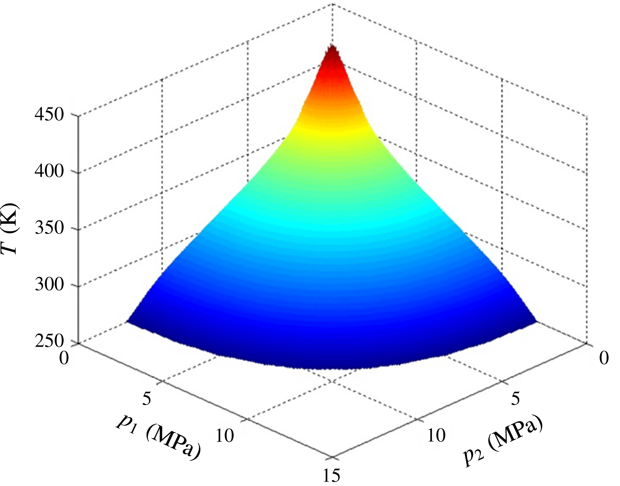
As an example, we investigate the non-ideal gas effect of methane. The equation of state and the pressure dependency of viscosity come from Younglove & Ely (Reference Younglove and Ely1987) and Setzmann & Wagner (Reference Setzmann and Wagner1991) respectively. The surface in figure 1 presents the pressure and temperature conditions when
 $\unicode[STIX]{x1D708}(p_{char})=\unicode[STIX]{x1D708}^{id}(\bar{p})$
. If (
 $p_{1},p_{2},T$
) is located below the surface, then
 $\unicode[STIX]{x1D708}(p_{char})<\unicode[STIX]{x1D708}^{id}(\bar{p})$
, indicating
 $\unicode[STIX]{x1D6FE}$
is positive and the non-ideal gas effect promotes the flow. Above the surface
 $\unicode[STIX]{x1D6FE}$
is negative, indicating the non-ideal gas effect restrains the flow. Thus, the previous controversy about whether the non-ideal gas effect promotes (Wu et al.
Reference Wu, Chen and Li2015) or restrains (Ren et al.
Reference Ren, Guo, Guo and Wang2015) the flow is quantitatively clarified.
The upstream pressure, downstream pressure and temperature conditions for methane when
 $\unicode[STIX]{x1D6FE}$
equals 0 (i.e.
 $\unicode[STIX]{x1D6FE}=0$
on the surface). If (
 $p_{1},p_{2},T$
) is located below the surface, the non-ideal gas effect promotes the flow; otherwise the non-ideal gas effect restrains the flow.

3 Simulation methods and validations
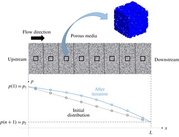
We employ independent numerical simulations to validate and demonstrate the theoretical analysis. A multiscale scheme is necessary for studying high Kn non-ideal gas flows in microporous media. On the one hand, the high Kn gas flow requires a pore-scale simulation to accurately capture the gas slip on the wall surfaces of the complex porous geometry. For example, the geometries of shales are quite different from those of sandstones and therefore the popular permeability models, which may work well for sandstones, are not valid for shales. On the other hand, the non-ideal gas effect manifests at the macroscale (e.g. core scale or field scale) where a significant pressure change exists, thus it is hardly well captured in the pore-scale simulation domain. Therefore the coupling of these two effects requires solving the gas flow at two scales simultaneously. Such a multiscale numerical scheme has been developed by Wang et al. (Reference Wang, Guo and Wang2016), which is illustrated in figure 2.
The multiscale numerical scheme for gas flow simulation. The porous media is divided into
 $n$
blocks (divided by the dashed lines). In each block, the small representative elementary volume (REV) at the centre (shown by the squares) can represent the flow resistance characteristics of each block. The gas flow in the REV is fully simulated by the lattice Boltzmann method at pore scale with all effects coupled.

Consider a field-scale porous media with gas flowing from upstream to downstream driven by a pressure difference. At this scale, the system can be simplified as a one-dimensional gas flow problem. When we consider the gas compressibility and the non-ideal gas effects, the pressure distribution along the flow direction is not linear. Suppose the porous media can be divided into several blocks with homogeneous transport properties in each one. Figure 2 shows
 $n$
blocks distinguished by dashed lines (
 $n=16$
in the following simulations). Under the assumption of homogeneous properties in each block, we can just do the pore-scale modelling in a representative elementary volume (REV) at the centre of each block (the squares in figure 2), which is much smaller compared to the block but can still represent the flow resistance characteristics. The number of blocks should be large enough to ensure the pressure distribution in each block is approximately linear, thus the pressure boundaries of each REV can be obtained by linear interpolation.
The flowchart of the multiscale numerical scheme is described as follows.
First an initial linear pressure distribution is given along the flow direction, as shown by the straight line in figure 2. The iteration between the field-scale and the pore-scale modelling has four steps. Step (i) determines the pressure boundaries of each REV by interpolation from the field pressure distribution. Step (ii) calculates the apparent permeability
 $K(i)$
of each REV by pore-scale simulation using an efficient lattice Boltzmann method. Step (iii) updates the pressure at the boundaries of each block based on the apparent permeability of the REV by
 $$\begin{eqnarray}p^{new}(i)=\frac{p(i-1)C(i-1)+p(i+1)C(i)}{C(i-1)+C(i)},\quad i=2,3,\ldots ,n,\end{eqnarray}$$
where
 $C(i)$
is the conductivity, defined as
 $$\begin{eqnarray}C(i)=\frac{Q_{m}}{\unicode[STIX]{x1D735}p}=\frac{K(i)}{\unicode[STIX]{x1D708}(i)}.\end{eqnarray}$$
Step (iv) checks the deviation between the new pressure distribution and the old one. Go back to step (i) if the deviation is greater than the tolerance.
The lattice Boltzmann method (LBM) is adopted for pore-scale simulation. LBM has two advantages: (i) LBM is derived from the Boltzmann equation (He & Luo Reference He and Luo1997; Chen & Doolen Reference Chen and Doolen1998), thus has a solid foundation for high Kn flow; (ii) LBM has a high efficiency for complex boundaries of porous structures (Wang & Chen Reference Wang and Chen2007; Wang et al. Reference Wang, Pan, Wang and Chen2007a ). Here we only list the important fundamentals of LBM and the details of the algorithm can be found in our previous work (Wang et al. Reference Wang, Guo and Wang2016).
LBM solves the evolution of the discrete distribution function:
 $$\begin{eqnarray}f_{i}(\boldsymbol{x}+\boldsymbol{c}_{i}\unicode[STIX]{x0394}t,t+\unicode[STIX]{x0394}t)-f_{i}(\boldsymbol{x},t)=\unicode[STIX]{x1D6FA}_{i},\quad i=0,1,\ldots ,N-1,\end{eqnarray}$$
where
 $f_{i}$
(
 $\boldsymbol{x},t$
) is the discrete distribution function,
 $\boldsymbol{c}_{i}$
the lattice speed,
 $\unicode[STIX]{x1D6FA}_{i}$
the discrete collision operator and
 $N$
the number of discrete velocities. The D3Q19 (three dimensions nineteen speeds) model and multiple relaxation time model (MRT) (Higuera, Succi & Benzi Reference Higuera, Succi and Benzi1989; Lallemand & Luo Reference Lallemand and Luo2000) are adopted for good numerical accuracy (d’Humières et al.
Reference d’Humières, Ginzburg, Krafczyk, Lallemand and Luo2002; Pan, Luo & Miller Reference Pan, Luo and Miller2006; Wang & Kang Reference Wang and Kang2009). For the MRT model, the discrete collision operator is expressed as
 $$\begin{eqnarray}\unicode[STIX]{x1D6FA}_{i}=-\mathop{\sum }_{j}(\unicode[STIX]{x1D648}^{-1}\unicode[STIX]{x1D64E}\unicode[STIX]{x1D648})_{ij}(f_{j}-f_{j}^{eq}).\end{eqnarray}$$
Here
 $\unicode[STIX]{x1D648}$
is a
 $19\times 19$
constant matrix (d’Humières et al.
Reference d’Humières, Ginzburg, Krafczyk, Lallemand and Luo2002),
 $\unicode[STIX]{x1D64E}$
is a diagonal matrix related to Kn (Pan et al.
Reference Pan, Luo and Miller2006) and
 $f_{i}^{eq}$
is the equilibrium distribution (Guo, Zheng & Shi Reference Guo, Zheng and Shi2008). After the discrete distribution function is calculated by (3.3), the flow density and velocity are determined as
 $$\begin{eqnarray}\unicode[STIX]{x1D70C}=\mathop{\sum }_{i}f_{i},\quad \boldsymbol{u}=\frac{1}{\unicode[STIX]{x1D70C}}\mathop{\sum }_{i}\boldsymbol{c}_{i}\,f_{i}.\end{eqnarray}$$
For boundary treatments, we apply a pressure boundary at the inlet and outlet (Guo, Zheng & Shi Reference Guo, Zheng and Shi2002) and a periodic boundary in the other directions. For no-slip gas flows, the classical bounce-back boundary is adopted at the solid surface. For high Kn flows, we followed the scheme of Li et al. (Reference Li, He, Tang and Tao2011), adopting a diffusive wall boundary (Ansumali & Karlin Reference Ansumali and Karlin2002) and an effective viscosity correction (Beskok & Karniadakis Reference Beskok and Karniadakis1999). Two geometries are considered in the following simulations: a two-dimensional channel and a three-dimensional porous structure which is large enough and periodic, and the repetitive unit serves as the REV (illustrated by the blue structure in figure 2). The structure is randomly reconstructed by the quartet structure generation set (QSGS) method (Wang et al. Reference Wang, Wang, Pan and Chen2007b ; Wang & Pan Reference Wang and Pan2008) and the detailed processes and parameters can be found in our previous work (Wang et al. Reference Wang, Guo and Wang2016).
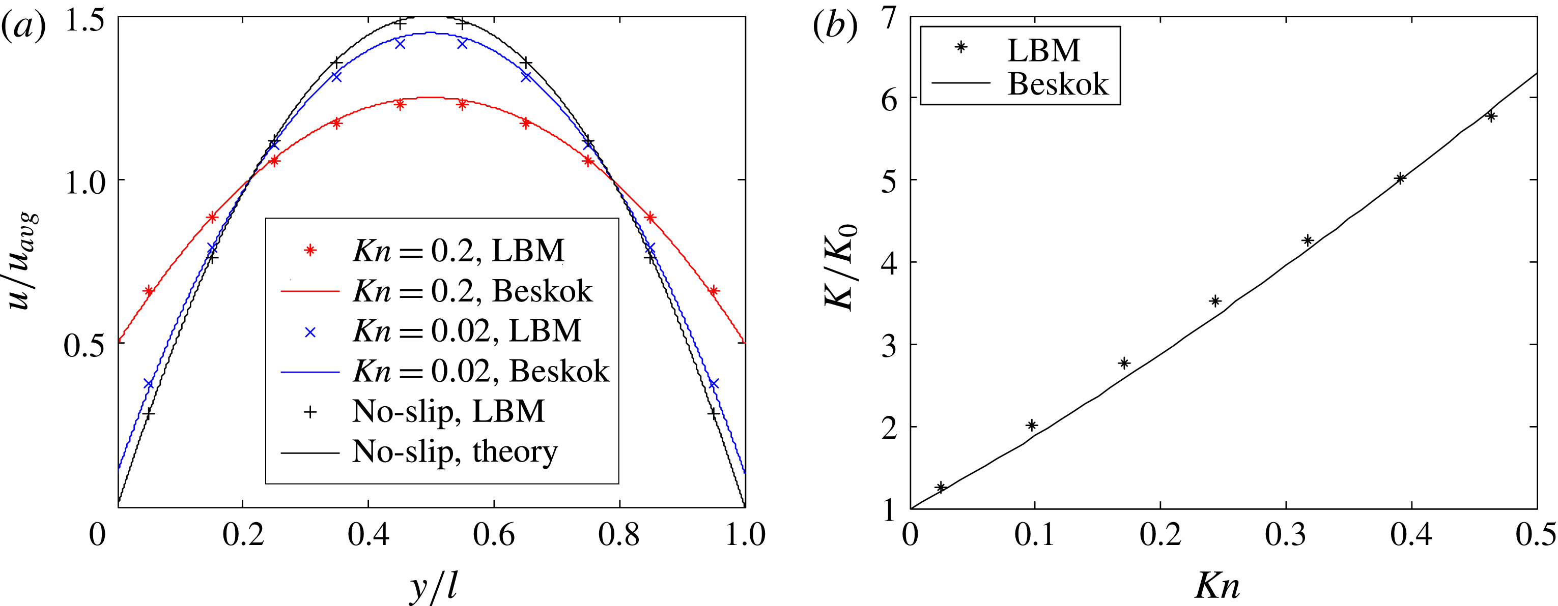
LBM simulation results of high Kn flow in channels compared with Beskok’s model. (a) Normalized velocity profiles; (b) apparent permeability normalized by intrinsic permeability
 $K_{0}=l^{2}/12$
, for which the average relative error of LBM modelling to Beskok’s model is 4 %.

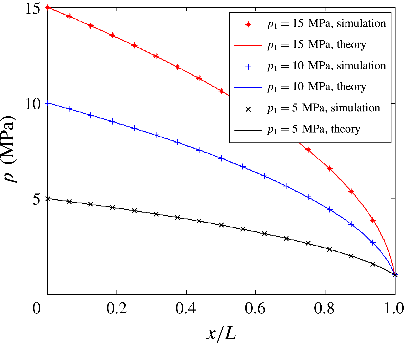
The pressure profiles of no-slip ideal gas flow in a long channel with different upstream pressures. Symbols represent the simulation results and lines are the theoretical solutions.

To validate the pore-scale LBM simulation, gas flows in a nanochannel driven by very small pressure difference are simulated. The normalized velocity profile across the channel and the apparent permeability agree well with Beskok’s model (Beskok & Karniadakis Reference Beskok and Karniadakis1999) in figure 3. To validate the multiscale numerical scheme, a no-slip ideal gas flow in a long channel is considered. The downstream pressure is 1 MPa while the upstream pressure varies from 5, 10 to 15 MPa. Figure 4 shows that the pressure profiles along the channel agree well with the theoretical solution:
 $$\begin{eqnarray}p^{2}=-(p_{1}^{2}-p_{2}^{2})x/L+p_{1}^{2}.\end{eqnarray}$$
4 Results and discussion
The four types of coupling between the high Kn effect and the non-ideal gas effect are demonstrated and validated by two examples. By comparing theoretical analysis and numerical simulation, the physical meaning of
 $\unicode[STIX]{x1D6FE}$
is explained concretely. For simplicity, the flow is in a long channel, whose height is in nanometres while the length is in metres, to represent the pore scale and field scale, respectively.
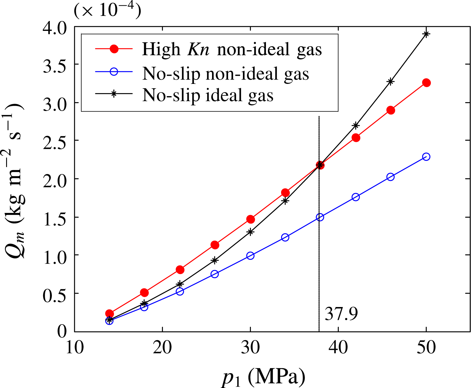
Simulation results of steady-state methane flow in a long channel. When upstream pressure is 37.9 MPa, the mass flux of high Kn non-ideal gas flow equals that of the no-slip ideal gas flow.

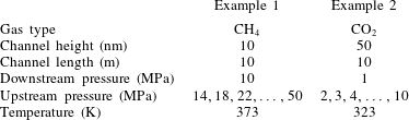
The first example is steady-state flow of methane with conditions similar to deep-seated shale gas flowing through nanopores (table 2). Three cases are considered: the high Kn non-ideal gas flow, the no-slip non-ideal gas flow and the no-slip ideal gas flow. For each case, the mass flux at different upstream pressures is obtained by multiscale simulation (figure 5). To reveal the mechanism, the problem is then independently analysed in theory. The characteristic viscosity
 $\unicode[STIX]{x1D708}(p_{char})$
and
 $\unicode[STIX]{x1D708}^{id}(\bar{p})$
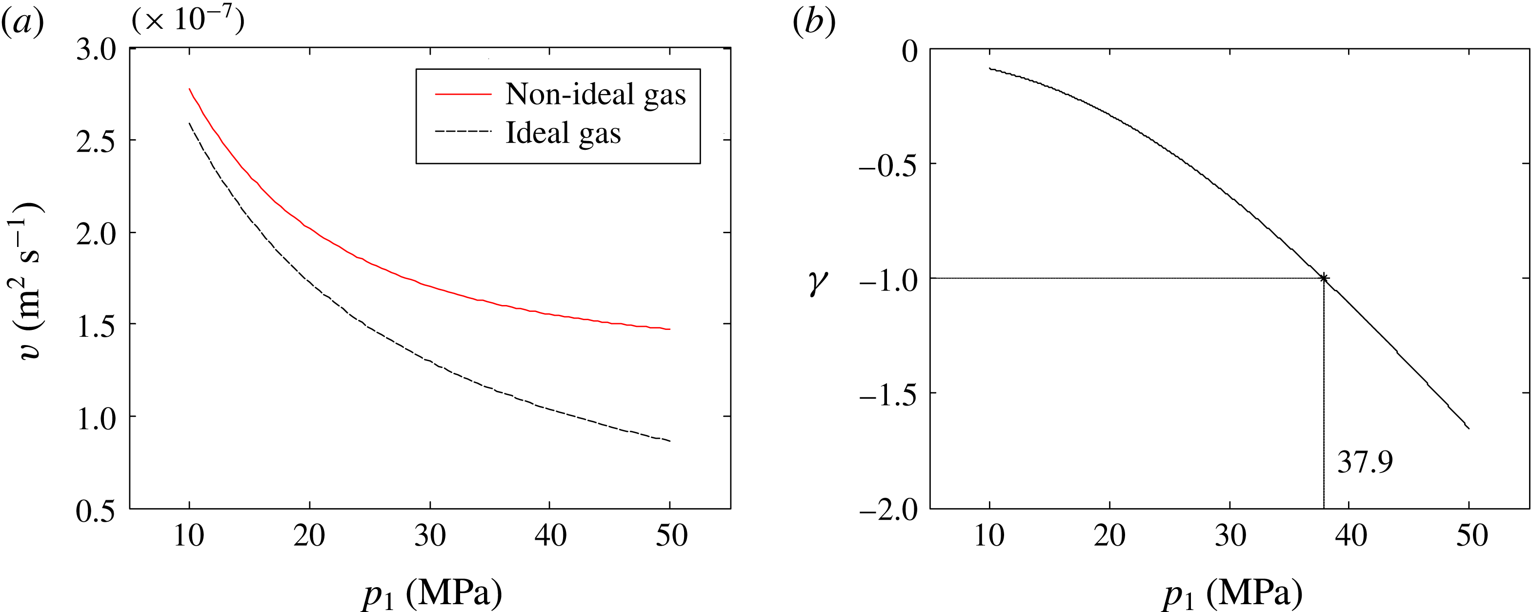
are computed by (2.9) and (2.14), respectively (figure 6
a). Since
 $\unicode[STIX]{x1D708}(p_{char})>\unicode[STIX]{x1D708}^{id}(\bar{p})$
, the non-ideal gas effect restrains the flow. This is confirmed in the simulation that the mass flux is decreased when the non-ideal gas effect is considered (figure 5). Substituting
 $\unicode[STIX]{x1D708}(p_{char})$
and
 $\unicode[STIX]{x1D708}^{id}(\bar{p})$
into (2.16), the dimensionless factor
 $\unicode[STIX]{x1D6FE}$
is calculated and presented in figure 6(b). Note that the slip factor
 $b$
in (2.16), which is the slope of
 $K/K_{0}$
versus Kn, is obtained by linear fitting of Beskok’s model (figure 3
b) for
 $0<Kn<0.5$
. When the upstream pressure
 $p_{1}<37.9$
MPa,
 $-1<\unicode[STIX]{x1D6FE}<0$
, indicating that the high Kn effect dominates over the non-ideal gas effect, their coupling promotes the flow (figure 6
b). Correspondingly, in the same pressure range the high Kn non-ideal gas flow has a higher mass flux than the no-slip ideal gas flow (figure 5). On the contrary, when the upstream pressure
 $p_{1}>37.9$
MPa,
 $\unicode[STIX]{x1D6FE}<-1$
, indicating that the non-ideal gas effect dominates over the high Kn effect, their coupling restrains the flow.
Theoretical analysis for methane flow. (a) The characteristic viscosity
 $\unicode[STIX]{x1D708}(p_{char})$
for non-ideal gas and
 $\unicode[STIX]{x1D708}^{id}(\bar{p})$
for ideal gas. (b) The dimensionless factor
 $\unicode[STIX]{x1D6FE}$
, which equals
 $-1$
when the upstream pressure is 37.9 MPa.

Physical conditions of the gas flow simulation in channel.

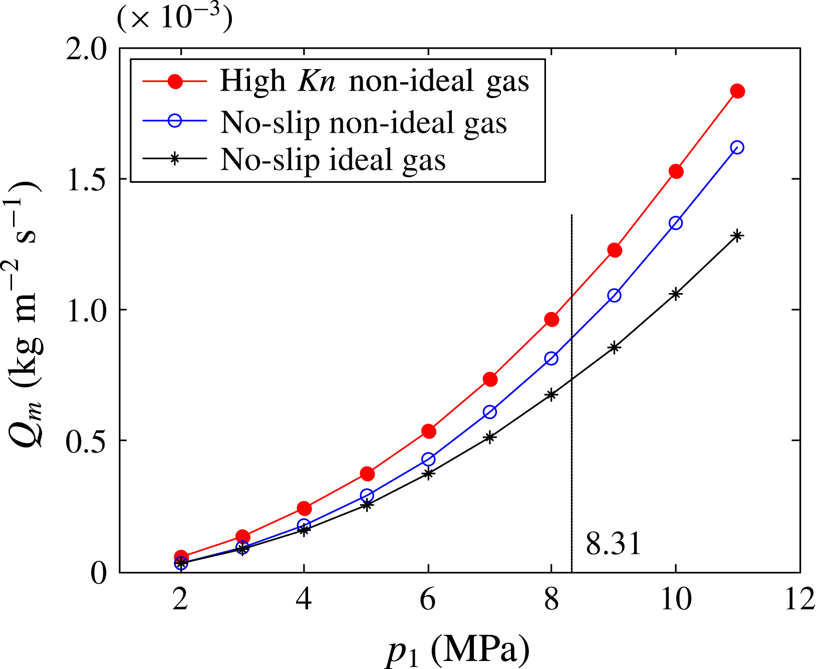
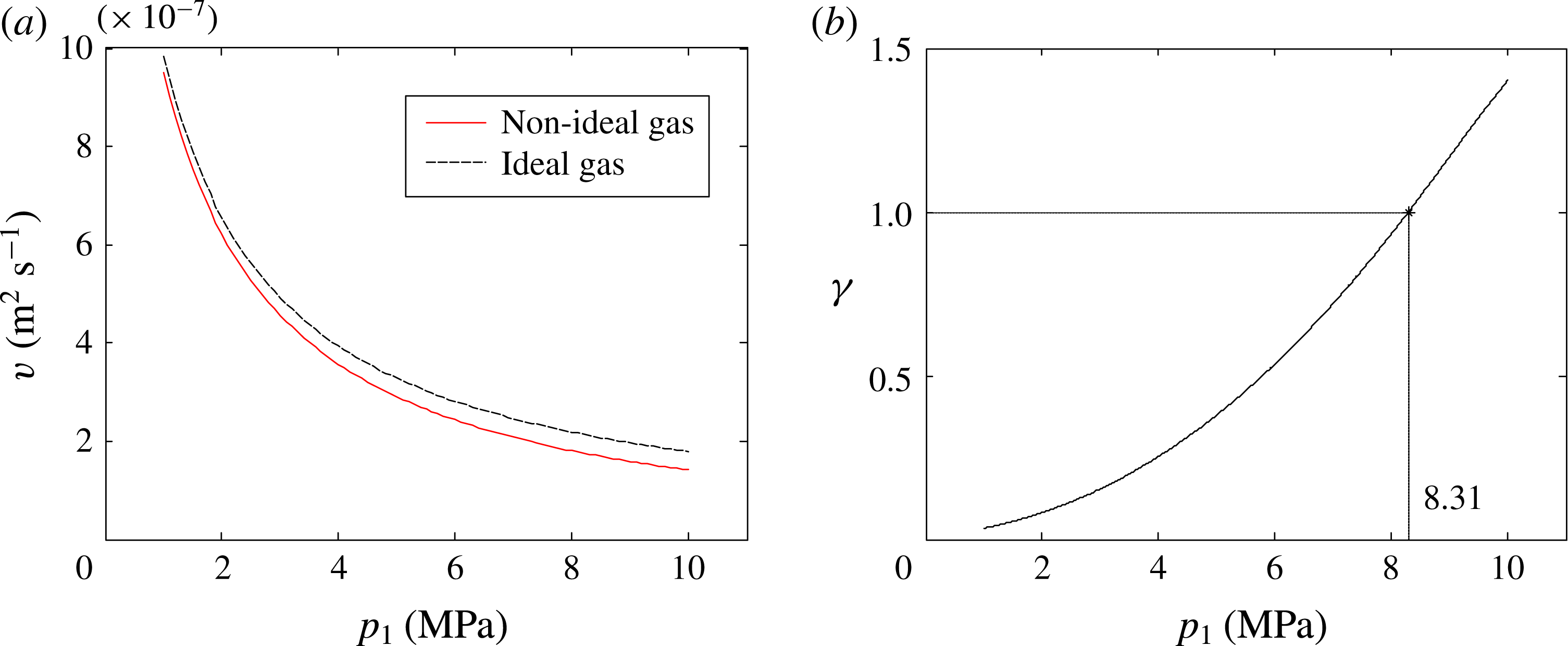
The next example is the steady-state flow of carbon dioxide with conditions similar to carbon dioxide sequestration (table 2). As before, the flow is investigated by both numerical simulations and theoretical analysis, whose results are shown in figures 7 and 8 respectively. For carbon dioxide, the characteristic viscosity
 $\unicode[STIX]{x1D708}(p_{char})$
is lower than
 $\unicode[STIX]{x1D708}^{id}(\bar{p})$
, indicating that the non-ideal gas effect promotes the flow (figure 8
a). This is confirmed by simulation that the mass flux is elevated when the non-ideal gas effect is considered (figure 7). Then we calculate the dimensionless factor
 $\unicode[STIX]{x1D6FE}$
by (2.16). When the upstream pressure
 $p_{1}<8.31$
MPa,
 $0<\unicode[STIX]{x1D6FE}<1$
, indicating that the high Kn effect dominates over the non-ideal gas effect (figure 8
b). Correspondingly, in the simulation, the elevation of mass flux caused by the high Kn effect is larger when
 $p_{1}<8.31$
MPa (figure 7). When the upstream pressure
 $p_{1}>8.31$
MPa, both simulation and theoretical analysis suggest that the non-ideal gas effect is dominant.
Simulation results for steady-state carbon dioxide flow in a long channel. When upstream pressure is 8.31 MPa, the mass flux elevated by the high Kn effect and the non-ideal gas effect is the same.

Theoretical analysis for carbon dioxide flow. (a) The characteristic viscosity
 $\unicode[STIX]{x1D708}(p_{char})$
for non-ideal gas and
 $\unicode[STIX]{x1D708}^{id}(\bar{p})$
for ideal gas. (b) The dimensionless factor
 $\unicode[STIX]{x1D6FE}$
, which equals 1 when the upstream pressure is 8.31 MPa.

With these two examples, it is proved that the dimensionless factor
 $\unicode[STIX]{x1D6FE}$
describes well the relative importance of the non-ideal gas effect and the high Kn effect. Note that, although the analysis is based on the steady state, the four types of coupling between the high Kn effect and the non-ideal gas effect also exist in non-steady-state flows. In the appendix, the pseudo-steady-state flow (Ahmed & McKinney Reference Ahmed and McKinney2005; Wang & Economides Reference Wang and Economides2009) is simulated by our multiscale numerical scheme (Wang et al.
Reference Wang, Guo and Wang2016). The results suggest that the classification of coupling works well for the pseudo-steady-state flow as well.
5 Characteristic pressure model for permeability calculation
We have clarified the coupling mechanism of the high Kn effect and the non-ideal gas effect in gas flows through porous media. In this section, the analysis is applied to laboratory measurement of rock core samples. The flow rate versus pressure conditions can be measured directly in the experiment, while the gas permeability is really needed in reservoir engineering. Therefore an accurate model is crucial to calculate the permeability from the measured flow rate. In fact, all of the effects which may influence the flow rate are mixed in experiments, including the gas compressibility, the high Kn effect and the non-ideal gas effect. When calculating gas permeability, the previous researchers usually use the ideal gas model (Klinkenberg Reference Klinkenberg1941) or adopt an averaged dynamic viscosity and compressibility factor for real gases (Rushing et al. Reference Rushing, Newsham, Lasswell, Cox and Blasingame2004; Gensterblum et al. Reference Gensterblum, Ghanizadeh and Krooss2014). Here, we propose a theoretical model to calculate the gas permeability from measured data, which accurately incorporates the high Kn effect and the non-ideal gas effect.
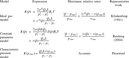
Models for the calculation of apparent gas permeability.

Equation (2.12) gives the gas apparent permeability at the characteristic pressure:
 $$\begin{eqnarray}K(p_{char})=\frac{Q_{m}L\unicode[STIX]{x1D708}(p_{char})}{p_{1}-p_{2}},\end{eqnarray}$$
where
 $\unicode[STIX]{x1D708}(p_{char})$
is the characteristic viscosity and
 $p_{char}$
is the characteristic pressure. Before applying the model,
 $\unicode[STIX]{x1D708}(p_{char})$
and
 $p_{char}$
need to be determined by (2.9) using the gas properties. After substituting the measured mass flux into (5.1), the apparent permeability at characteristic pressure is predicted.
Table 3 compares our characteristic pressure model with two previous popular models for gas permeability. One model was proposed by Klinkenberg, and is based on the ideal gas assumption (Klinkenberg Reference Klinkenberg1941). The other assumes constant dynamic viscosity
 $\unicode[STIX]{x1D707}$
and compressibility factor
 $Z$
at the arithmetical mean pressure
 $\bar{p}$
for the real gas (Rushing et al.
Reference Rushing, Newsham, Lasswell, Cox and Blasingame2004). The results show that the previous models are not very accurate for strong gas non-ideality. The error is caused by the difference between the characteristic pressure and the mean pressure, as well as the kinematic viscosity difference from an ideal gas (table 3). A quantitative estimation of gas non-ideality for several popular gases has been provided by Monte Carlo simulations in our previous work (Wang et al.
Reference Wang, Lan and Li2008), based on which we can know when the new model is necessary.
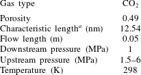
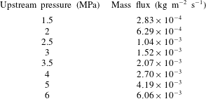
To test these models, high Kn non-ideal gas flow in a rock core is simulated by the multiscale method. The simulation serves as a substitute of a real experiment, from which mass flux is read and used as input for the models in table 3. To make the simulation close to the real experiments, the structure is a three-dimensional random structure (illustrated by the blue structure in figure 2) reconstructed by the QSGS method (Wang et al. Reference Wang, Wang, Pan and Chen2007b ; Wang & Pan Reference Wang and Pan2008). The pressure and temperature conditions are also at the same level as in the laboratory (table 4). The mass flux is then substituted into the three models (table 3) to calculate the apparent gas permeability. To evaluate the models, the gas permeability is also obtained directly from pore-scale simulation, in which a very small pressure difference is applied to a single reconstructed structure (the blue structure in figure 2) to drive the gas flow. Based on the mass flux and the corresponding pressure gradient, the apparent permeability is calculated by Darcy’s law in (2.1). Since the permeability is defined from Darcy’s law, this calculation is used as the standard. Several pore-scale simulations are conducted with a pressure range from 1 MPa to 5 MPa, to obtain the reference apparent permeability at different pressures.
Conditions of the gas flow simulation in reconstructed rock core.

a Characteristic length is calculated as twice the pore volume divided by the interface area (Civan Reference Civan2010).
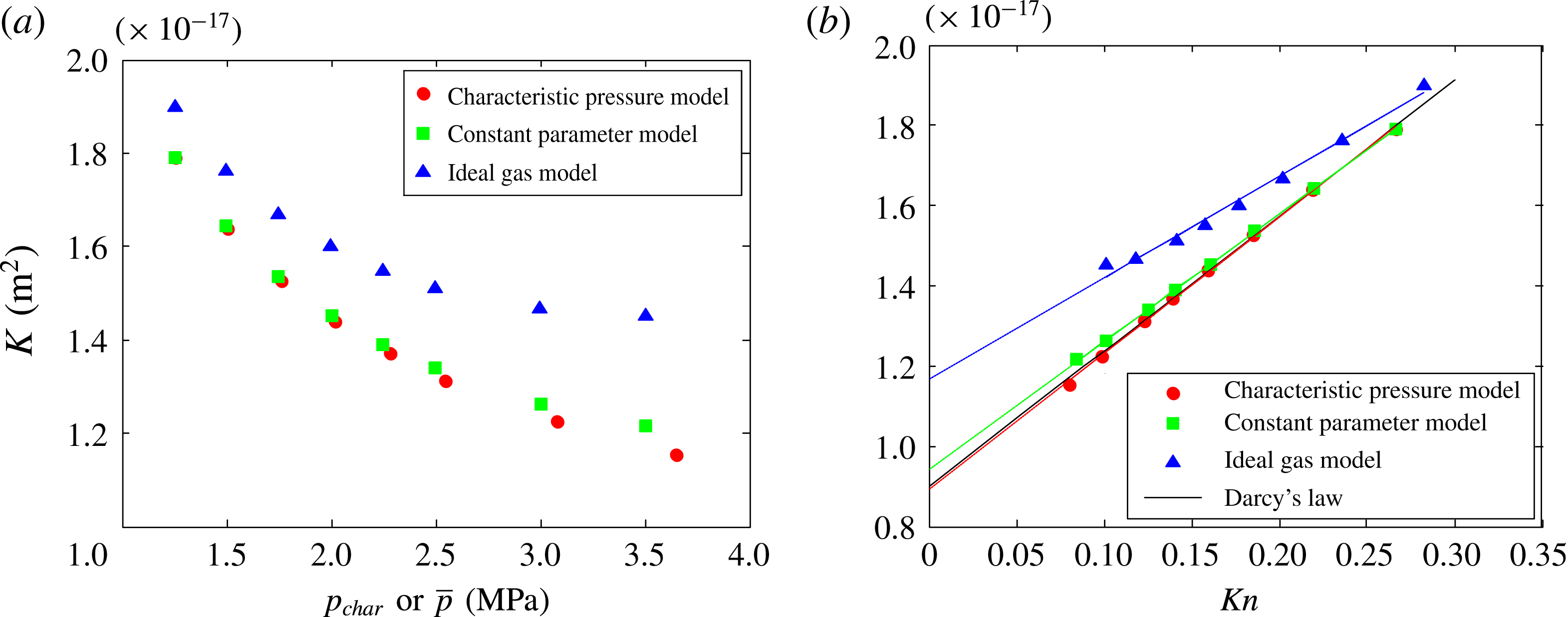
Substituting the simulated mass flux (table 5) into the three models, the apparent permeability at the characteristic pressure (predicted by characteristic pressure model) or mean pressure (predicted by constant parameter model and ideal gas model) is presented in figure 9(a). Then the Kn at these pressures is calculated by (2.5) and (2.6) using the data from table 4, and the apparent permeability is plotted against Kn (figure 9 b). Meanwhile, the gas permeability obtained accurately from Darcy’s law is also presented in figure 9(b) as the standard. Among the three models, the apparent permeability predicted by the characteristic pressure model is the best. By linearly fitting the apparent permeability against the Kn in figure 9(b), the intrinsic permeability and the slip factor are obtained by (2.4), as well as the relative errors (table 6).
The apparent permeability of the reconstructed rock core predicted by the three models. (a) Apparent permeability predicted by the new model at characteristic pressure and by the previous models at mean pressure. (b) Apparent permeability versus Kn. The predictions are compared to the permeability obtained from pore-scale simulation using Darcy’s law. The results are linearly fitted to compute intrinsic permeability and slip factor.

Results of the gas flow simulation in reconstructed rock core.

The intrinsic permeability and slip factor predicted by the three models and the accurate results from pore-scale simulation.

Because of the strong non-ideality of carbon dioxide, the permeability predicted by the ideal gas model is not reliable. For the ideal gas model, the linearity of the apparent permeability data in figure 9(b) is not good and the errors of the intrinsic permeability and slip factor are large. For the constant parameter model, the error using constant
 $\unicode[STIX]{x1D707}$
and
 $Z$
at the mean pressure is within 10 %, which is generally acceptable for engineering applications. In contrast, the characteristic pressure model is much better, with an error approximately one order of magnitude lower than the constant parameter model and two orders lower than the ideal gas model.
6 Conclusions
We conduct a rigorous analysis of the coupling of high Kn and non-ideal gas effects for gas flows in microporous media. The complicated non-ideal gas behaviour is characterized by two parameters: the characteristic pressure and the characteristic viscosity. A dimensionless factor is proposed to quantify the coupling mechanism of the high Kn effect and non-ideal gas effect. The coupling is divided into four types according to its value, depending on whether the non-ideal gas effect promotes the flow and the relative importance of the two effects. To validate and demonstrate the theoretical results, gas flows in a long channel are numerically simulated. The four coupling types are clearly shown by two examples and the divisions between different types agree very well with theoretical predictions. Further, the analysis is applied to the laboratory measurement of rock core samples. A characteristic pressure model is proposed to accurately calculate the gas permeability, which fully incorporates the high Kn effect and the non-ideal gas effect. The error of the new model is approximately one order of magnitude lower than the constant parameter model and two orders lower than the ideal gas model. With better accuracy, the characteristic pressure model can bridge the laboratory experiments and the reservoir engineering.
Acknowledgements
This work is financially supported by the NSFC-DFG Collaboration Grant (no. 11761131012), the NSF grant of China (no. U1562217) and National Science and Technology Major Project on Oil and Gas (no. 2017ZX05013001).
Appendix
In this appendix, the pseudo-steady-state flow is studied to demonstrate that the four types of coupling between the high Kn effect and non-ideal gas effect also exist in non-steady-state flow. A pseudo-steady state may occur during the boundary dominated flow period, which is at the late stage of gas exploitation (Wang & Economides Reference Wang and Economides2009; MoradiDowlatabad & Jamiolahmady Reference MoradiDowlatabad and Jamiolahmady2017). Recently, this flow type has been applied to the production prediction of multi-fractured horizontal wells, which is essential for shale gas exploitation (Guo, Wang & Zhang Reference Guo, Wang and Zhang2016; Wei et al. Reference Wei, Duan, Dong and Fang2016; MoradiDowlatabad & Jamiolahmady Reference MoradiDowlatabad and Jamiolahmady2017). Pseudo-steady state assumes that the pressure drops at a constant rate at every point of the field, and there is no flux at the drainage boundary (Ahmed & McKinney Reference Ahmed and McKinney2005; Wang & Economides Reference Wang and Economides2009). Following the method in our previous work (Wang et al. Reference Wang, Guo and Wang2016), pseudo-steady-state gas flow in a long channel is simulated.
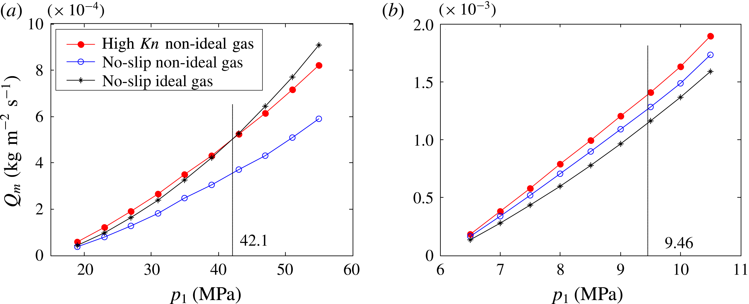
Downstream mass flux of pseudo-steady-state gas flow in a long channel. (a) Methane: when upstream pressure is 42.1 MPa, the mass flux of high Kn non-ideal gas flow equals that of the no-slip ideal gas flow. (b) Carbon dioxide: when upstream pressure is 9.46 MPa, the mass flux elevated by the high Kn effect and the non-ideal gas effect is the same.

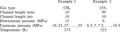
Physical conditions of the pseudo-steady-state gas flow simulation.

As before, methane and carbon dioxide are used in simulation to demonstrate the four types of coupling. The physical conditions are listed in table 7 and the simulation results are presented in figure 10. For methane, the non-ideal gas effect restrains the flow. When the upstream pressure
 $p_{1}<42.1$
MPa, the high Kn effect dominates over the non-ideal gas effect; otherwise the non-ideal gas effect dominates. For carbon dioxide, the non-ideal gas effect promotes the flow. When the upstream pressure
 $p_{1}>9.46$
MPa, the high Kn effect dominates over the non-ideal gas effect; otherwise the non-ideal gas effect dominates.