


1 Introduction
Understanding the fundamental physics of a solidifying aqueous binary fluid is important in a wide range of sciences, including geophysics, oceanography, metallurgy and electrical engineering (Chalmers Reference Chalmers1964; Rosenberger Reference Rosenberger1979; Loper & Roberts Reference Loper, Roberts and Soward1983; Hobbs Reference Hobbs2010). When a binary fluid is cooled and solidified from a horizontal plane boundary, the growing solid phase can form a dendritic structure of crystals called a mushy layer (see Part 1, Ding, Wells & Zhong (Reference Ding, Wells and Zhong2019), for a more detailed discussion). Mushy layers are reactive porous materials with interstitial melt that can flow in response to externally applied forces. The dynamics of the interstitial flow is resisted by the porous structure, which depends on the local solid fraction
 $\unicode[STIX]{x1D719}$
, the volume ratio of the solid to the mixture. The porosity
 $1-\unicode[STIX]{x1D719}$
is simply related to the solid fraction.
Since the liquid and solid phases have different thermal and mechanical properties (such as heat conductivity, heat capacity, etc.), the field equations that describe the evolution of temperature and melt concentration within the mushy layers involve governing parameters strongly dependent on
 $\unicode[STIX]{x1D719}$
. Accurate information about
 $\unicode[STIX]{x1D719}$
, including its variation in both space and time, thus plays a crucial role in improving modelling of mushy-layer growth. Early theoretical work by Huppert & Worster (Reference Huppert and Worster1985) considered the solid fraction as an important parameter in the governing equations for mushy-layer growth. This pioneering theoretical model treated the mushy layer as a continuum, with the physical properties of the solid and liquid being averaged over the mush region. It predicted the growth rate, temperature and concentration profiles of mushy layers that were in agreement with experimental results. In more advanced theoretical models (e.g. Worster Reference Worster1986, Reference Worster1991) predictions were made for the solid fraction evolving in space and time. The large specific surface area allows interstitial gradients of heat and solute to relax rapidly to a state of local thermodynamic equilibrium, with the temperature and concentration in the liquid pore space coupled via a liquidus constraint. Then, knowledge of the bulk phase-weighted concentration and temperature is sufficient to predict the solid fraction
 $\unicode[STIX]{x1D719}$
(see Worster (Reference Worster2000), for a summary). Thus macroscopic temperature changes or solute transport through the mushy layer can modify the solid fraction. A particularly striking modification of solid fraction arises from convective flow within the mushy layer, which can dissolve solid-free channels or chimneys in the mushy layer, through which buoyant plumes of fluid drain into the neighbouring fluid region (see reviews by Worster (Reference Worster1997) and Zhong et al. (Reference Zhong, Fragoso, Wells and Wettlaufer2012)). This process is sometimes called gravity drainage, and is a primary mechanism for solute fluxes from a growing mushy layer (Notz & Worster Reference Notz and Worster2009) providing a coupled feedback on mushy layer solid fraction and permeability. Experimental studies of the solid fraction with adequate resolution in both space and time will advance our understanding of the fluid dynamics involved in solidifying binary fluids.
Due to the fact that mushy layers are porous materials that consist of solid crystals, they are optically opaque. Direct measurements of the solid fraction in mushy layers through optical methods are challenging. Moreover, since growing mushy layers have a three-dimensional dendritic structure on multiple scales (Huppert Reference Huppert1990; Golden et al.
Reference Golden, Eicken, Heaton, Miner, Pringle and Zhu2007) determining
 $\unicode[STIX]{x1D719}$
through statistical analysis of experimental data requires high-resolution measurement, and it is particularly challenging to capture porosity evolution during growth. In early experimental studies, Chen & Chen (Reference Chen and Chen1991) and Chen (Reference Chen1995) applied X-ray tomography to measure the solid fraction in a mushy layer using a post-mortem measurement after solidifying an aqueous ammonium chloride solution. It was observed that the solid fraction decreases significantly towards the mush–liquid interface. Wettlaufer, Worster & Huppert (Reference Wettlaufer, Worster and Huppert1997) determined the time evolution of the vertically averaged solid fraction in an aqueous sodium chloride mushy layer by measuring the volumetric change during solidification due to the density difference between water and ice. A variety of experimental systems have been used to show that the melting of a reactive mixed-phase region can result in solidification deeper within that region as a result of convection, and investigated the evolution of the solid fraction (Hallworth & Huppert Reference Hallworth and Huppert2004; Hallworth, Huppert & Woods Reference Hallworth, Huppert and Woods2005; Yu et al.
Reference Yu, Bergman, Huguet and Alboussiere2015; Huguet et al.
Reference Huguet, Alboussiere, Bergman, Deguen, Labrosse and Lesceur2016). Several authors (Shirtcliffe, Huppert & Worster Reference Shirtcliffe, Huppert and Worster1991; Chiareli & Worster Reference Chiareli and Worster1992; Notz, Wettlaufer & Worster Reference Notz, Wettlaufer and Worster2005) developed methods to measure the electrical resistance in the melt, which varies with the local solid fraction and allows the evolution of
 $\unicode[STIX]{x1D719}(z)$
to be determined as it evolves during solidification. This method has been extended and employed for in situ field measurements of sea ice (Notz & Worster Reference Notz and Worster2008, Reference Notz and Worster2009) which is a geophysical example of a mushy layer. Such a method was also successfully applied to the growth of a mushy layer under high gravity (Huguet et al.
Reference Huguet, Alboussiere, Bergman, Deguen, Labrosse and Lesceur2016). Bulk concentration and solid fraction have also been inferred from measurements of the complex dielectric permittivity and temperature of sea ice using embedded probes (Backstrom & Eicken Reference Backstrom and Eicken2006), via surface impedance tomography (Sampson et al.
Reference Sampson, Golden, Gully and Worby2011) or via electromagnetic induction (Hunkeler et al.
Reference Hunkeler, Hendricks, Hoppmann, Farquharson, Kalscheuer, Grab, Kaufmann, Rabenstein and Gerdes2015). Aussillous et al. (Reference Aussillous, Sederman, Gladden, Huppert and Worster2006) used magnetic resonance imaging to study how the fine structure and solid fraction evolve during solidification of a mushy layer. The solid fraction increases in the lower part of the layer after the onset of internal convection. Finally, we note that a range of post-mortem measurements have been taken from cores of sea ice, which is necessarily destructive, as the sample is removed for analysis. Solid fraction can be inferred from measured ice temperature, assumed local thermodynamic equilibrium and bulk salinity measured from melted slices of the sample (e.g. see discussion in Hunke et al.
Reference Hunke, Notz, Turner and Vancoppenolle2011), or via scanning methods using magnetic resonance imaging or micro-computed tomography (e.g. Eicken et al.
Reference Eicken, Bock, Wittig, Miller and Poertner2000; Lieb-Lappen, Golden & Obbard Reference Lieb-Lappen, Golden and Obbard2017).
Despite a variety of methods having been attempted, very few high-resolution measurements have been made to determine the distribution of solid fraction and its evolution in growing mushy layers through well-controlled laboratory experiments. To date, all such measurements used either destructive post-mortem sampling, freezing of instruments into a growing mushy layer, or encounter difficulties of growing small samples of mushy layer within the confines of an imaging scanner. In this paper, we report experimental studies of the profiles of solid fraction
 $\unicode[STIX]{x1D719}$
in a mushy layer formed when an aqueous ammonium chloride solution is cooled from below with a periodically varying boundary temperature. We measure the local temperature
 $T(z,t)$
at various heights within the mushy layer, and characterize how the phases of temperature oscillations propagate from the bottom boundary through the mushy layer, and how the amplitude decays with height. We show that the decay rate of the thermal oscillation decreases with an increasing initial concentration
 $C_{0}$
, but the propagation speed of the oscillation phases increases with
 $C_{0}$
. These behaviours are consistent with an increase in solid fraction which enhances the thermal conductivity but reduces the specific heat of the mushy layer. Using high-resolution measurements of
 $T(z,t)$
we present a method for determining the distribution of solid fraction
 $\unicode[STIX]{x1D719}(z)$
for various
 $C_{0}$
, based on the dependence of thermal material properties on
 $\unicode[STIX]{x1D719}$
. Our analysis of the time-dependent heat transport equation reveals that when the mush temperature varies periodically in response to the modulation of the cooling boundary, the increment of the fluid internal energy can be appropriately correlated to the local conductive heat transports, as presented in a heat-flux diagram. With these experimental findings, we extract accurate results of the local thermal diffusivity and hence determine the distribution of the solid fraction
 $\unicode[STIX]{x1D719}(z)$
in the mushy layer. Our approach provides a method to estimate solid fraction using only measurements of temperature within the mushy layer.
In the next section, we summarize the apparatus, experimental methods and procedures that are described in more detail in Part 1 (Ding et al. Reference Ding, Wells and Zhong2019), which considered the early-time growth characteristics of a mushy layer with the boundary temperature modulated periodically in time. In § 3 we describe experimental measurements of temperature during the corresponding late-time period of mushy-layer growth, where the mushy layer is modulated about a nearly steady background state. The results compare well to a simplified theoretical model for thermal wave propagation due to diffusive heat transfer with uniform material properties (derived in appendix B). In § 4 we analyse heat transfer within the mushy layer, outlining an algorithm to estimate the solid fraction via the thermal properties, and investigate how the solid fraction varies in space and time. The mean solid fraction estimated from mushy-layer temperature variation compares well to an independent estimate from global solute conservation and measurements of concentration in the overlying liquid. In § 5 we summarize the results and discuss the implications for future work.
2 Experimental methods
The construction of the apparatus and the experimental environment have been described in detail in Part 1 (Ding et al.
Reference Ding, Wells and Zhong2019). Here we briefly review the experimental procedure, and introduce the experimental components and methods that are relevant to our temperature and concentration measurements. A thermally shielded 80 mm
 $\times$
80 mm
 $\times$
150 mm tank of aqueous
 $\text{NH}_{4}\text{Cl}$
solution is cooled from below, with the bottom temperature
 $T_{b}(t)=T_{b,0}+A\sin (\unicode[STIX]{x1D714}t+\unicode[STIX]{x1D719}_{0})$
controlled and modulated over time
 $t$
about a background temperature
 $T_{b,0}$
, with amplitude
 $A$
, angular frequency
 $\unicode[STIX]{x1D714}$
and initial phase
 $\unicode[STIX]{x1D719}_{0}$
. A vertically stacked array of thermistors measures temperature
 $T(z,t)$
at different heights
 $z$
in the mushy layer, and shadowgraphy images were analysed to infer the mush thickness
 $h(t)$
. See Part 1 (Ding et al.
Reference Ding, Wells and Zhong2019) for further details on the configuration, methods used and procedure for initializing the experiment.
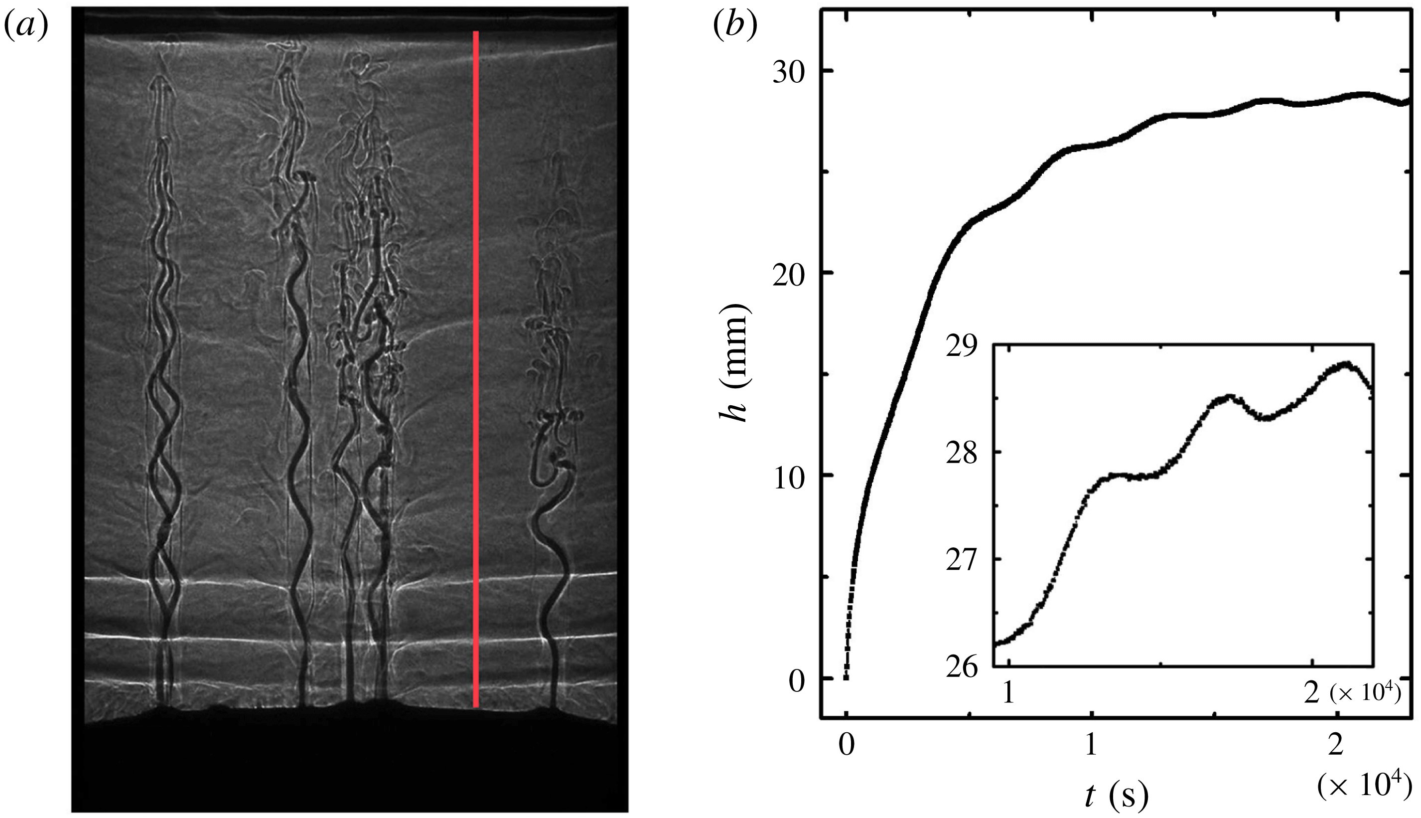
Fluid concentration and temperature within the liquid region were measured using a dual probe consisting of a four-electrode microscale conductivity sensor and a thermocouple (MSCTI, Precision Measurement Engineering, model 125). The probe was mounted on a computer-controlled positioner. Its conductivity sensor and the thermocouple junction were located at the same vertical level and 3 mm apart horizontally. When measuring the vertical profiles of
 $C(z)$
and
 $T(z)$
, the dual probe traversed vertically through the liquid region at a constant speed of
 $0.4~\text{mm}~\text{s}^{-1}$
(figure 1
a). Both the conductivity and temperature signals were recorded at a sampling frequency of 1 Hz, yielding a vertical resolution of 0.4 mm for each profile. In each profile measurement the probe travelled 80 mm, taking 200 s. Such a time span is at least one order of magnitude less than the modulation period
 $\unicode[STIX]{x1D70F}=2\unicode[STIX]{x03C0}/\unicode[STIX]{x1D714}$
, and is much less than the time scale of mushy-layer growth. During the measurements data were always recorded while the probe was traversed downwards, with the two sensors ahead of the probe holder, to minimize any disturbances in the measured region. Several scans were made within each modulation period to determine the mean solid fractions
 $\langle \unicode[STIX]{x1D719}\rangle$
as we discuss in § 4.4.
The conductivity sensor and the thermocouple were calibrated before and after each experiment against
 $\text{NH}_{4}\text{Cl}$
solutions of known concentrations at various temperatures that cover the entire experimental parameter range, with an accuracy of 0.1 wt% in concentration and 0.02 K in temperature. The voltage signal of the thermocouple was first turned into temperature using a fitted six-order polynomial function. The output voltage from the conductivity sensor was then translated into concentration based on the calibrated conductivity–concentration relations (Head Reference Head1983). Measurements of
 $C(z)$
and
 $T(z)$
were made in late modulation periods with
 $t\geqslant 5\unicode[STIX]{x1D70F}$
with mush temperature measurements performed at the same time. In these late periods, our temperature measurements indicate that the thermal properties and hence the porosity structure of the mushy layers show no long-term trend, with the signal repeatable between modulation periods (figures 2 and 10). As discussed in § 4.4, we estimate the mean solid fraction
 $\langle \unicode[STIX]{x1D719}\rangle$
in the mushy region, applying conservation of solute and using the concentration profile measured in the liquid region. These results for
 $\langle \unicode[STIX]{x1D719}\rangle$
are compared with an alternative estimated based on our temperature measurements within the mushy layers.
Various initial liquid concentrations
 $C_{0}$
were initially investigated. For a better resolution in measuring the mushy-layer thickness
 $h(t)$
and the mush temperature
 $T(z,t)$
, we chose
 $C_{0}$
in the range of
 $26~\text{wt}\%\leqslant C_{0}\leqslant 32~\text{wt}\%$
. The solution was prepared at an initial temperature
 $T_{0}$
above the liquidus temperature
 $T_{0}>T_{L}(C_{0})$
to avoid crystallization prior to the experiment.
3 The mushy-layer growth and the temperature distribution
(a) Shadowgraph image that shows the mush region (black area near the bottom), narrow salt-finger plumes near the mush–liquid interface, wider plumes rising from chimneys and the double-diffusive layers in the liquid region. The image is captured at the beginning of the sixth modulation period in an experiment with initial concentration
 $C_{0}=29~\text{wt}\%$
,
 $A=10~\text{K}$
and
 $\unicode[STIX]{x1D70F}=4000~\text{s}$
. The vertical red line marks the path along which the MSTCI probe traverses when temperature and salinity measurements are taken in the liquid region. (b) The mushy-layer height
 $h$
as a function of time. Inset: a segment of
 $h(t)$
from the fourth to the sixth modulation periods.
The dynamical growth of mushy layers in early periods of periodic cooling has been discussed in Part 1 (Ding et al.
Reference Ding, Wells and Zhong2019) revealing modulation of the mushy-layer thickness around a background state in the absence of modulation. The experimental data of the mushy-layer thickness
 $h(t)$
were shown to be broadly consistent with theoretical predictions from a numerical model of mushy-layer growth. In this section we present measurements of
 $h(t)$
and the temperature distribution
 $T(z,t)$
within the mushy layers at relatively late modulation periods when the mushy layer nearly approaches a constant thickness. We also discuss how temperature oscillations propagate through the mushy layer in this state.
Time series of temperature at various heights
 $T(z,t)$
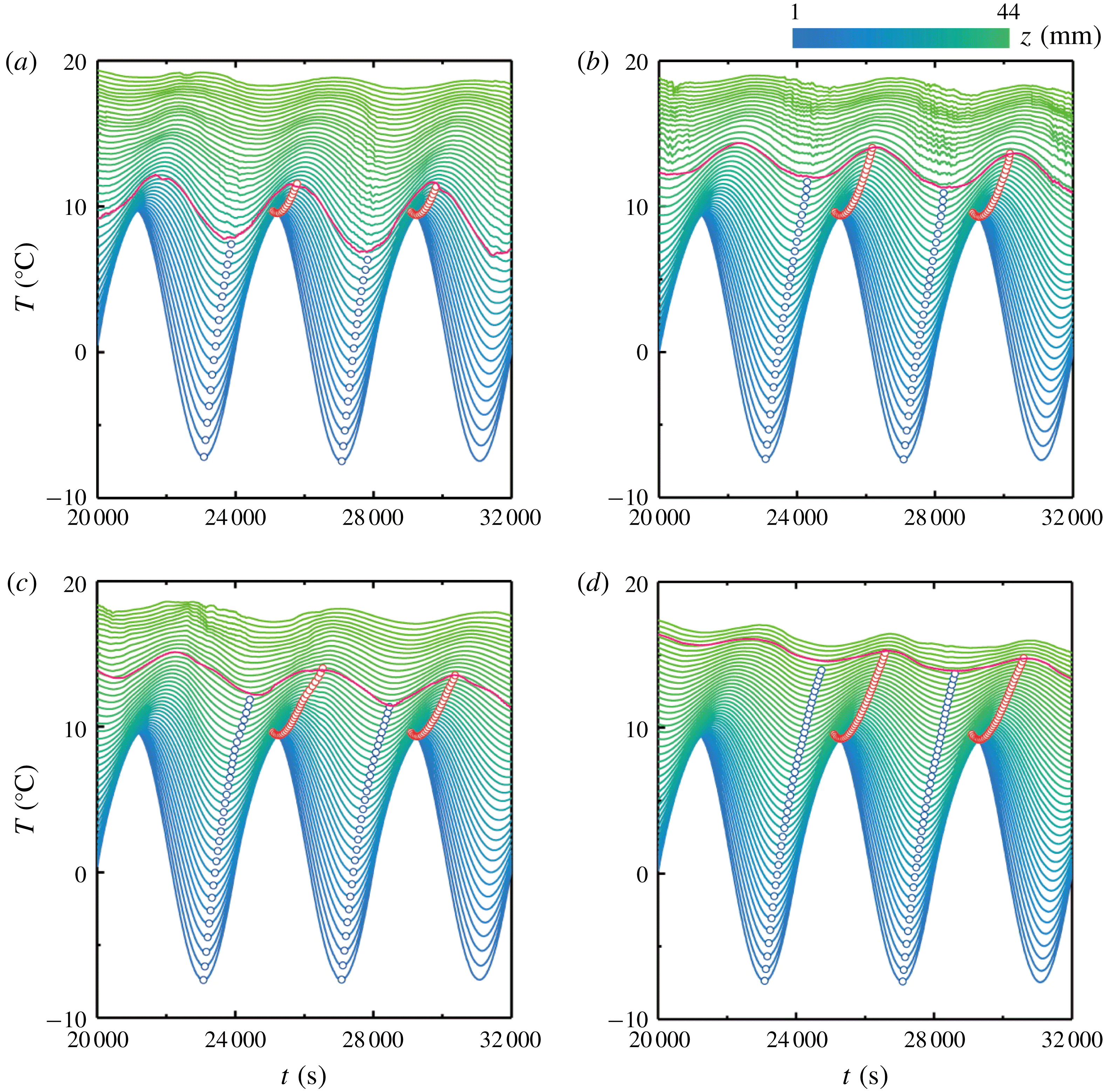
measured from the fifth to the seventh modulation period. The coloration represents the height on a linear scale, as indicated by the upper colour bar. The red curve shows the position of the mush–liquid interface. Local minima and maxima of
 $T(z,t)$
in the mush region are marked by blue and red circles, respectively. Results for
 $A=10~\text{K}$
and
 $\unicode[STIX]{x1D70F}=4000~\text{s}$
, with initial concentration
 $C_{0}$
of (a) 26 wt%, (b) 28 wt%, (c) 30 wt% and (d) 32 wt%.
The shadowgraph image in figure 1(a) presents the typical morphology of the mushy-layer and flow structures in the liquid region during the late modulation periods. As is commonly seen when
 $\text{NH}_{4}\text{Cl}$
–
 $\text{H}_{2}\text{O}$
solutions are cooled from below (e.g. see review by Zhong et al.
Reference Zhong, Fragoso, Wells and Wettlaufer2012) the shadowgraph reveals multiple buoyant solute-depleted plumes rising from chimneys in the mushy layer, with smaller solute-depleted plumes near the mush–liquid interface. In § 4.4 we suggest that the white near-horizontal bands in the background fluid are likely the result of double-diffusive layering due to the cold plumes cooling a solute stratification. Formation of double-diffusive layers has also been observed in earlier experiments of solidification of a mushy layer (Beckermann & Viskanta Reference Beckermann and Viskanta1988; Chen Reference Chen1997). The speed at which the mush–liquid interface advances towards the liquid region is obtained through our image processing method using a sequence of shadowgraph images (see discussions in Part 1, Ding et al. (Reference Ding, Wells and Zhong2019)). Figure 1(b) depicts results of the mushy-layer height
 $h(t)$
from an experiment with an initial concentration
 $C_{0}=29~\text{wt}\%$
. It is clearly seen that oscillations appear in
 $h(t)$
about a background growth curve which at early times is reminiscent of the scaling
 $h_{0}(t)\propto t^{1/2}$
characteristic of diffusive growth into a deep fluid layer with constant basal cooling. In the later periods the oscillation amplitude decays and the mean of
 $h(t)$
finally becomes nearly independent of time (inset of figure 1
b) with small oscillations about a nearly steady state. As we will elucidate in detail in the following sections, during the late growth periods convective heat transport through the mushy layer becomes negligible. Therefore the growth of the mushy layer is dictated mainly by thermal conduction and its advance speed is determined by the thermal gradient at the mush–liquid interface. The mush thickness eventually reaches a statistically steady state where the heat flux from the mush balances the turbulent heat flux from compositional convection at the mush–liquid interface. Modulated by the cooling boundary, the mush temperature and thus the thermal gradient varies periodically in time with a nearly constant mean, and gives rise to the periodic oscillations of the growth curve
 $h(t)$
.
To gain further insights into the growth of the mushy layer, we examine the spatial and temporal evolution of the mush temperature
 $T(z,t)$
during late modulation periods. Figure 2 shows the fluid temperature measured at various different heights for four initial fluid concentrations. The time traces of temperature show the prominent feature of periodic oscillations, with oscillation amplitudes and phases dependent on height. They demonstrate propagation of thermal oscillations with substantial decay through the mushy layer. For a quantitative analysis, we determine the amplitudes and phases of the temperature oscillation by the maxima (minima) in
 $T(z,t)$
, marked by the red (blue) circles in figure 2. The temperature amplitude,
 $\unicode[STIX]{x1D6FF}T=T_{p}-T_{v}$
, is given by the difference between the maximum (
 $T_{p}$
) and minimum (
 $T_{v}$
) temperature within one oscillation period. The phase of oscillation,
 $\unicode[STIX]{x1D6FF}\unicode[STIX]{x1D719}=2\unicode[STIX]{x03C0}[t(T_{v})-t(T_{b,v})]/\unicode[STIX]{x1D70F}$
, is defined as the phase difference between
 $T_{v}$
and the cooling boundary temperature
 $T_{b}(t)$
. Results of
 $\unicode[STIX]{x1D6FF}T$
and
 $\unicode[STIX]{x1D6FF}\unicode[STIX]{x1D719}$
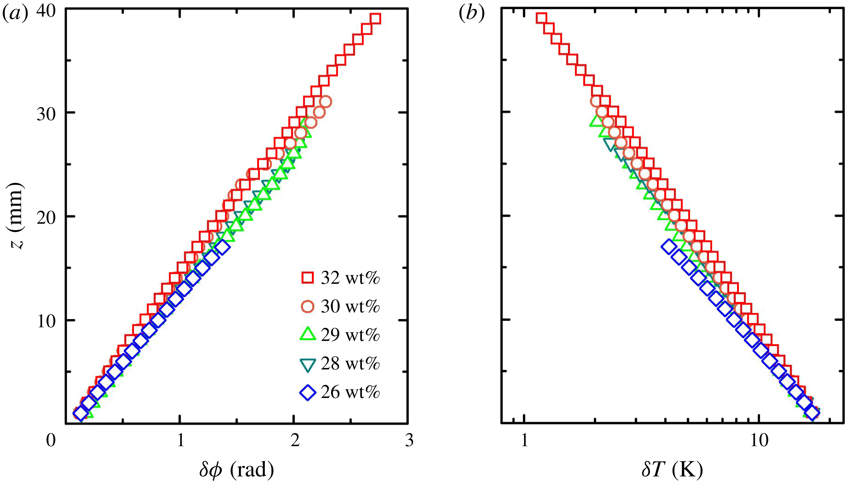
at different mush heights are depicted in figure 3. We see that at late times the oscillation phase of
 $T(z,t)$
lags behinds
 $T_{b}(t)$
, and
 $\unicode[STIX]{x1D6FF}\unicode[STIX]{x1D719}$
increases almost linearly with increasing mush height
 $z$
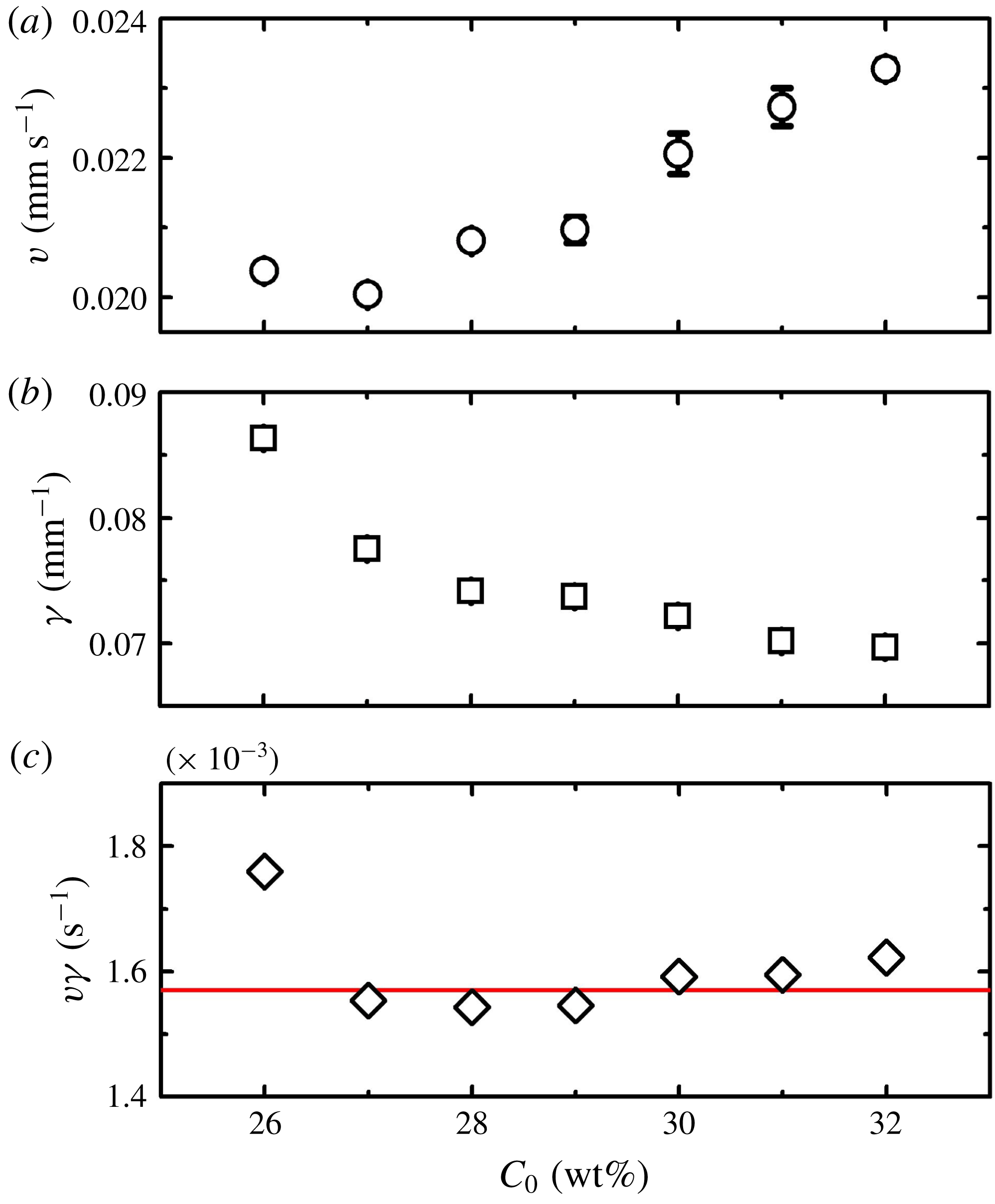
. Thus, thermal oscillations propagate with a constant velocity through the mushy layer. The propagation speed,
 $v=\unicode[STIX]{x1D714}\,\text{d}z/\text{d}(\unicode[STIX]{x1D6FF}\unicode[STIX]{x1D719})$
, is determined by the slope of the phase-lag profile
 $\unicode[STIX]{x1D6FF}\unicode[STIX]{x1D719}(z)$
and depicted as a function of the initial concentration
 $C_{0}$
in figure 4(a). The oscillation amplitudes in
 $T(z,t)$
are shown to decrease exponentially with increasing height within the mush:
 $\unicode[STIX]{x1D6FF}T\propto \text{e}^{-\unicode[STIX]{x1D6FE}z}$
(figure 3
b). The decay rates of the amplitude
 $\unicode[STIX]{x1D6FE}$
are determined by the profiles of
 $\unicode[STIX]{x1D6FF}T(z)$
. Results of
 $\unicode[STIX]{x1D6FE}$
for various
 $C_{0}$
are shown in figure 4(b).
Properties of temperature oscillations in
 $T(z,t)$
as functions of the mushy-layer height for various initial concentrations. (a) The phase lags between the minima of
 $T(z,t)$
and the cooling boundary temperature
 $T_{b}(t)$
. (b) The peak-to-trough temperature amplitude
 $\unicode[STIX]{x1D6FF}T=T_{p}-T_{v}$
. Data are measured from the fifth to the sixth modulation period and extracted from the temperature traces shown in figure 2, for different concentrations.
In appendix B we describe a simplified theoretical calculation with assumed constant material properties. Modulation with small amplitude
 $A\ll \unicode[STIX]{x0394}T_{0}=T_{b,0}-T_{L}(C_{i})$
and high-frequency modulation compared to the time scale of diffusion,
 $\unicode[STIX]{x1D714}h_{0}^{2}/\unicode[STIX]{x1D6FC}\gg 1$
, produces a long-time solution
 $$\begin{eqnarray}\displaystyle T=T_{b,0}+\unicode[STIX]{x0394}T_{0}\frac{z}{h_{0}}+A\text{e}^{-z\sqrt{\unicode[STIX]{x1D714}/2\unicode[STIX]{x1D6FC}}}\sin \left(\unicode[STIX]{x1D714}t-z\sqrt{\frac{\unicode[STIX]{x1D714}}{2\unicode[STIX]{x1D6FC}}}+\unicode[STIX]{x1D719}_{0}\right), & & \displaystyle\end{eqnarray}$$
where
 $C_{i}$
is the concentration at the mush–liquid interface,
 $h_{0}$
is the steady-state mushy-layer thickness at long times in the absence of modulation and
 $\unicode[STIX]{x1D6FC}$
is the thermal diffusivity of the mushy layer (here assumed to be spatially uniform). The time-dependent perturbation to the steady state yields a classical thermal wave solution for diffusion with periodically modulated boundary temperature (cf. § 2.6 of Carslaw & Jaeger Reference Carslaw and Jaeger1959). This predicts a constant propagation speed
 $v=\sqrt{2\unicode[STIX]{x1D6FC}\unicode[STIX]{x1D714}}$
for the phase of the sinusoidal oscillations of temperature (giving rise to the nomenclature of a thermal wave). It also predicts exponential decay of the oscillation amplitude with height over the length scale
 $\unicode[STIX]{x1D6FE}^{-1}=\sqrt{2\unicode[STIX]{x1D6FC}/\unicode[STIX]{x1D714}}$
which corresponds to a length scale for diffusion over a modulation period. This captures the observed pattern of phase propagation and exponential decay of amplitude with height seen in figures 2 and 3. Furthermore, the theory predicts that the combination of scales
 $v\unicode[STIX]{x1D6FE}=\unicode[STIX]{x1D714}$
, which is independent of
 $\unicode[STIX]{x1D6FC}$
and other parameters. This is in reasonable agreement with the data in figure 4(c), where
 $\unicode[STIX]{x1D714}=1.57\times 10^{-3}~\text{rad}~\text{s}^{-1}$
is constant. The agreement seems surprisingly good, given that we have neglected variation of the material properties with
 $z$
, and that the assumption
 $A\ll \unicode[STIX]{x0394}T_{0}$
is rather marginal. Hence we conclude that the temperature evolution seen in figure 2 is consistent with a diffusive thermal wave superimposed on a background steady state, with the decay rate
 $\unicode[STIX]{x1D6FE}^{-1}=\sqrt{2\unicode[STIX]{x1D6FC}/\unicode[STIX]{x1D714}}$
and phase propagation velocity
 $v=\sqrt{2\unicode[STIX]{x1D6FC}\unicode[STIX]{x1D714}}$
varying with an effective diffusivity
 $\unicode[STIX]{x1D6FC}$
which depends on concentration
 $C_{0}$
. This suggests the propagation of temperature oscillations through a mushy layer is substantially influenced by the initial fluid concentration, since the latter may significantly alter the thermal properties of the mushy layer. In general, solidification of a binary aqueous solution with a higher initial concentration results in a mushy layer with larger mean solid fraction. Based on the volume-weighted average, the mean thermal conductivity of the mushy layer
 $k_{m}=k_{s}\unicode[STIX]{x1D719}+k_{l}(1-\unicode[STIX]{x1D719})$
becomes greater, and the specific heat
 $cp_{m}=cp_{s}\unicode[STIX]{x1D719}+cp_{l}(1-\unicode[STIX]{x1D719})$
is less, which increases the effective thermal diffusivity
 $\unicode[STIX]{x1D6FC}=k_{m}/cp_{m}$
. (Here the thermal conductivity
 $k$
and heat capacity per unit volume
 $cp$
have subscript
 $s$
in the solid phase, subscript
 $l$
in the liquid phase and subscript
 $m$
for the weighted value for the mushy layer.) Thus a larger concentration leads to thermal waves with a faster propagation speed and a smaller decay rate.
(a) Propagation speed of the thermal waves
 $v$
for different
 $C_{0}$
, where
 $v$
is determined by the initial slope of the phase-lag profiles
 $\unicode[STIX]{x1D6FF}\unicode[STIX]{x1D719}(z)$
shown in figure 3(a). (b) The decay rates
 $\unicode[STIX]{x1D6FE}$
of the amplitude of temperature oscillations for different
 $C_{0}$
calculated from figure 3(b). (c) Product of
 $v\unicode[STIX]{x1D6FE}$
as a function of
 $C_{0}$
. The red line shows the theoretical prediction
 $v\unicode[STIX]{x1D6FE}=\unicode[STIX]{x1D714}=1.57\times 10^{-3}~\text{rad}~\text{s}^{-1}$
.
Another notable feature of the mush temperature shown in figure 2 is that the evolution of
 $T(z,t)$
during one modulation period becomes highly repeatable at each height near the bottom cooling boundary. For a given
 $z$
, oscillations of the mush temperature are very close to periodic, with nearly identical amplitudes and phases in different modulation periods. The well-repeated temperature responses in the mushy layer to the applied thermal modulation indicate that there is no significant trend in the variation of local thermal properties in the mush over time. This is suggestive of either an approximately time-independent porosity structure in the mush region, particularly near the bottom cooling boundary, or else one that oscillates periodically in time. Such a stationary mush structure appears in the late growth periods when convection in the interstitial melt diminishes and the mushy layer becomes stagnant. This limits changes to the bulk concentration of the ice via gravity drainage, and creates an appropriate condition for studying the distributions of solid fraction through temperature measurements (see § 4).
Normalized vertical temperature profiles of the mushy layer
 $T^{\ast }(z^{\ast })=T/T_{i}(t)$
as a function of
 $z^{\ast }(t)=z/h(t)$
measured at four phases during the sixth modulation period. Filled symbols: data for
 $C_{0}=26~\text{wt}\%$
; open symbols: data for
 $C_{0}=29~\text{wt}\%$
. The inset sketches the variation of the bottom temperature in these four phases. Results for
 $A=10~\text{K}$
,
 $\unicode[STIX]{x1D70F}=4000~\text{s}$
.
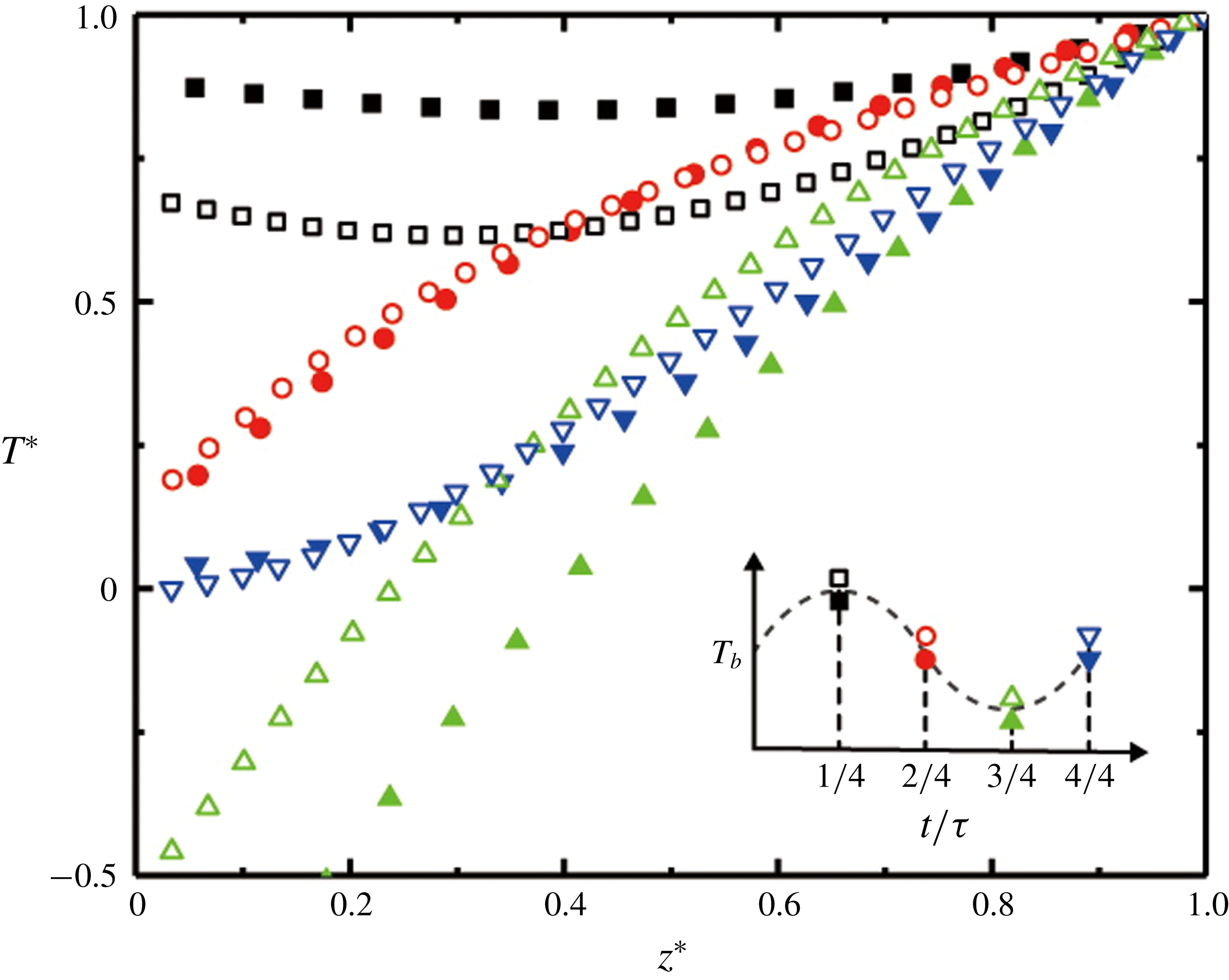
For a direct comparison of the temperature distribution in the mushy layers that grow from different initial concentrations, we present in figure 5 normalized vertical temperature profiles
 $T^{\ast }(z^{\ast })$
measured at four moments (
 $t=i/4\unicode[STIX]{x1D70F},i=1,2,3,4$
). Here the mush temperature is non-dimensionalized,
 $T^{\ast }(t)=(T(z,t)-T_{b,0})/(T_{i}(t)-T_{b,0})=T(z,t)/T_{i}(t)$
, with the mean cooling boundary temperature being
 $T_{b,0}=0\,^{\circ }\text{C}$
and
 $T_{i}(t)$
the temperature at the mush–liquid interface. The height is normalized by the mushy-layer thickness
 $z^{\ast }(t)=z/h(t)$
. Results for both
 $C_{0}=26$
and 29 wt% imply that variations of the mush-temperature profiles can be categorized into two phases that depend on variations of cooling boundary temperature
 $T_{b}$
. In a decreasing phase (
 $\unicode[STIX]{x1D70F}/4\leqslant t<3\unicode[STIX]{x1D70F}/4$
) when
 $T_{b}$
is decreasing in time, the slope of
 $T^{\ast }(z^{\ast })$
decreases with increasing height. Thus curves of
 $T^{\ast }(z^{\ast })$
in this phase are convex. However, when
 $T_{b}$
is increasing (
 $0\leqslant t<\unicode[STIX]{x1D70F}/4$
and
 $3\unicode[STIX]{x1D70F}/4\leqslant t<\unicode[STIX]{x1D70F}$
),
 $T^{\ast }(z^{\ast })$
is concave with slope increasing with
 $z^{\ast }$
. As discussed above, such a depth dependence of the mush temperature is due to the finite thermal diffusivity that causes time delays when the bottom-temperature oscillations diffuse through the mushy layer, with the phase lag of
 $T(z,t)$
behind
 $T_{b}(t)$
increasing when the height increases (see figure 3
a).
It is worth noting that a negative slope of
 $T^{\ast }(z^{\ast })$
appears at small mush heights when
 $T_{b}$
is near a maximum (
 $t=\unicode[STIX]{x1D70F}/4$
). A negative temperature gradient in the mushy layer is indicated as well in figure 2 near the maxima of
 $T(z,t)$
at low heights (where the time traces for different heights cross). We attribute this phenomenon to the mush temperature varying more rapidly near the base due to thermal modulations than the slower diffusive propagation of the temperature oscillations through the mushy layer to greater heights. This can be rationalized using the approximate thermal wave solution (3.1). Setting
 $\unicode[STIX]{x1D719}_{0}=0$
and letting
 $\unicode[STIX]{x1D6FE}=\sqrt{\unicode[STIX]{x1D714}/2\unicode[STIX]{x1D6FC}}$
, then from (3.1) the temperature gradient in the mushy layer is
 $$\begin{eqnarray}\displaystyle \frac{\unicode[STIX]{x2202}T}{\unicode[STIX]{x2202}z}=\frac{\unicode[STIX]{x0394}T_{0}}{h_{0}}-\unicode[STIX]{x1D6FE}A\text{e}^{-\unicode[STIX]{x1D6FE}z}[\sin (\unicode[STIX]{x1D714}t-\unicode[STIX]{x1D6FE}z)+\cos (\unicode[STIX]{x1D714}t-\unicode[STIX]{x1D6FE}z)]. & & \displaystyle\end{eqnarray}$$
For a given depth
 $z$
, this has a minimum value
 $\unicode[STIX]{x0394}T_{0}/h_{0}-\sqrt{2}\unicode[STIX]{x1D6FE}A\text{e}^{-\unicode[STIX]{x1D6FE}z}$
at times
 $\unicode[STIX]{x1D714}t-\unicode[STIX]{x1D6FE}z=\unicode[STIX]{x03C0}/4+2n\unicode[STIX]{x03C0}$
for integers
 $n$
. For large enough values of
 $\unicode[STIX]{x1D6FE}A$
, the temperature gradient
 $\unicode[STIX]{x2202}T/\unicode[STIX]{x2202}z$
will be negative for small
 $z$
during an interval of time about
 $\unicode[STIX]{x1D714}t-\unicode[STIX]{x1D6FE}z\approx \unicode[STIX]{x03C0}/4+2n\unicode[STIX]{x03C0}$
. For example, for
 $C_{0}=29~\text{wt}\%$
, figure 4(b) gives
 $\unicode[STIX]{x1D6FE}=0.074~\text{mm}^{-1}$
whilst
 $A=10~\text{K}$
in figure 5, yielding
 $\unicode[STIX]{x1D6FE}A\sqrt{2}\approx 1.0~\text{K}~\text{mm}^{-1}$
, whilst
 $\unicode[STIX]{x0394}T_{0}/h_{0}\approx 0.5~\text{K}~\text{mm}^{-1}$
. Hence, the thermal wave solution predicts that
 $\unicode[STIX]{x2202}T/\unicode[STIX]{x2202}z|_{z=0}$
will be negative for a period of time centred around
 $t=\unicode[STIX]{x1D70F}/8$
into the modulation period. Note that periods with
 $\unicode[STIX]{x2202}T/\unicode[STIX]{x2202}z|_{z=0}<0$
will have a positive heat flux from the cooling plate into the mushy layer, despite the overall trend for cooling by the lower boundary. We further expect that this effect is more pronounced for low initial concentrations, when the background temperature gradient is smaller (cf. figure 2), and in experimental conditions with large modulation amplitude and frequency, when the thermal wave component dominates the variation of the mush temperature.
Results in figure 5 also suggest that the mush temperature profiles are dependent on the initial fluid concentration. Large deviations in
 $T^{\ast }(z^{\ast })$
are seen from the profiles with different
 $C_{0}$
when
 $T_{b}$
reaches a maximum (
 $t=\unicode[STIX]{x1D70F}/4$
) or a minimum (
 $t=3\unicode[STIX]{x1D70F}/4$
). For a lower
 $C_{0}$
the temperature span crossing the mushy layer
 $T_{i}-T_{b}$
is smaller due to the lower liquidus temperature
 $T_{i}=T_{L}(C_{i})$
, and hence there is a larger oscillation amplitude in the dimensionless temperature
 $T^{\ast }$
. When
 $T_{b}=0\,^{\circ }\text{C}$
(
 $t=2\unicode[STIX]{x1D70F}/4,4\unicode[STIX]{x1D70F}/4$
) profiles of
 $T^{\ast }(z^{\ast })$
for the two concentrations appear closer to each other. However, there are still notable differences between the two curves in these phases, indicative of differing thermal properties of the mushy layer due to the differing fluid concentrations. Finally we note that the variations of the profiles
 $T^{\ast }(z^{\ast })$
within one modulation cycle shown in figure 5 are typical and repeatable in different modulation periods (cf. figure 2).
4 Inferring the solid-fraction distribution in mushy layers
4.1 Heat transports within a mushy layer
In growing mushy layers, heat transport between the mush and the liquid region occurs mainly through two types of processes. At early times, convection mainly occurs at the mush–liquid interface in the form of small-scale salt fingers in the presence of a stabilizing thermal gradient. This boundary-mode convection is driven by the compositional gradient that is established due to the formation of a solute-depleted boundary layer ahead of the growing mushy layer. As the mushy layer grows and reaches a critical height, a second type of convection occurs as a result of a hydrodynamic instability due to density gradients within the mushy layer (Worster Reference Worster1992). In this mushy-layer mode convection, large-scale plumes emanate from solid-free chimneys dissolved in the interior of the mushy layer, in a process often called gravity drainage. Heat and solute transport through the mushy-layer mode convection plays an important role in determining the heat budget of growing mushy layers. During late growth periods, however, mushy-layer convection approaches an asymptotic state when the growth rate approaches zero (Tait & Jaupart Reference Tait and Jaupart1989). The time-integrated expulsion of light solution modifies the concentration in the liquid region and causes the liquid concentration
 $C_{l}$
just above the mushy layer to decrease. In the following we will demonstrate that convection driven by the buoyancy force within the mushy layer carries a negligible heat transport compared to thermal conduction within the mushy layer.
The governing equation of the temperature distribution
 $T(z,t)$
within a mushy layer reads
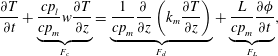 $$\begin{eqnarray}\displaystyle \frac{\unicode[STIX]{x2202}T}{\unicode[STIX]{x2202}t}+\underbrace{\frac{cp_{l}}{cp_{m}}w\frac{\unicode[STIX]{x2202}T}{\unicode[STIX]{x2202}z}}_{F_{c}}=\underbrace{\frac{1}{cp_{m}}\frac{\unicode[STIX]{x2202}}{\unicode[STIX]{x2202}z}\left(k_{m}\frac{\unicode[STIX]{x2202}T}{\unicode[STIX]{x2202}z}\right)}_{F_{d}}+\underbrace{\frac{L}{cp_{m}}\frac{\unicode[STIX]{x2202}\unicode[STIX]{x1D719}}{\unicode[STIX]{x2202}t}}_{F_{L}}, & & \displaystyle\end{eqnarray}$$
relevant to a vertical measurement profile located away from chimneys. The physical parameters are
 $cp$
the specific heat,
 $k$
the thermal conductivity and
 $L$
the latent heat. The subscripts
 $m$
and
 $l$
indicate the quantities in the mush and pure liquid region, respectively. The convective Darcy velocity
 $w$
arises in the mushy layer due to the gravity drainage. Previous theoretical and numerical modelling work suggests that significant horizontal thermal gradients occur in a narrow boundary layer near each chimney due to the cooling effect of cold solute-depleted plumes. However, the temperature gradient is predominantly vertical in the mushy layer further away from the chimneys (Wells, Wettlaufer & Orszag Reference Wells, Wettlaufer and Orszag2010; Rees Jones & Worster Reference Rees Jones and Worster2013). We have hence neglected horizontal temperature gradients for profiles taken outside of the chimneys and their associated thermal boundary layers. This heat equation expresses that temperature evolution in a mushy layer,
 $\unicode[STIX]{x2202}T/\unicode[STIX]{x2202}t$
, depends on heat-transport components including thermal advection
 $F_{c}$
, thermal conduction
 $F_{d}$
and the latent heat flux
 $F_{L}$
(all normalized by
 $cp_{m}$
). In the following, we estimate the magnitude of the convective heat transport
 $F_{c}$
and the latent heating
 $F_{L}$
, and their contribution to the heat budget of the system.
(a) Components of the heat equation estimated at the mid-height (
 $z=12~\text{mm}$
) of the mushy layer. Here the latent heating contribution
 $F_{L}=1.3\times 10^{-2}~\text{mK}~\text{s}^{-1}$
is determined by the difference of
 $\langle \unicode[STIX]{x1D719}\rangle$
measured in the fifth and sixth modulation periods, whilst the convective contribution
 $F_{c}$
is discussed further in the text. (b) Shadowgraph images illustrate the dynamical features of the plume flows from chimneys that undergo coiling instability. Results for an initial concentration
 $C_{0}=29~\text{wt}\%$
,
 $A=10~\text{K}$
and
 $\unicode[STIX]{x1D70F}=4000~\text{s}$
.
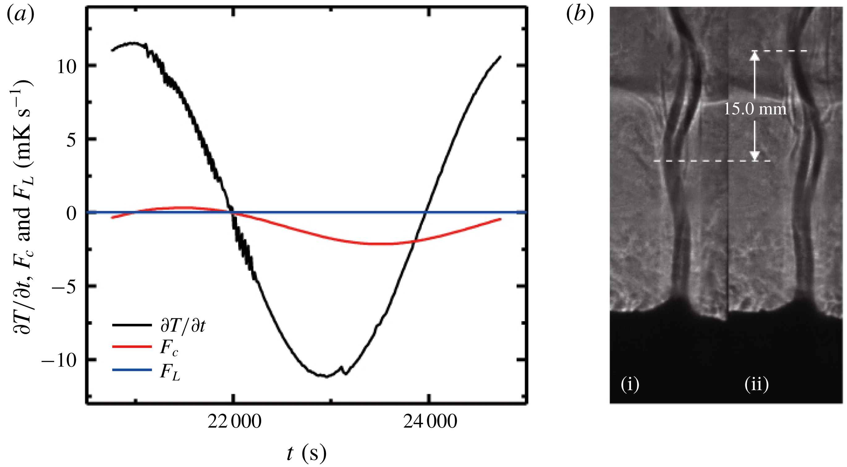
In order to estimate the convective heat transfer
 $F_{c}$
in a mushy layer, we estimate the fluid velocity of the large-scale plume flows from the chimneys. Figure 6(b) presents two snapshots of the plumes emanating from chimneys in the interior of the mushy layer, in which the upward wavy motion of the plumes is clearly seen. Assuming that the waves are generated by a generalization of the Kelvin–Helmholtz instability (following similar analysis of saline plumes; Pesci, Porter & Goldstein Reference Pesci, Porter and Goldstein2003), the vertical fluid velocity
 $W$
within the chimney plume can be determined through
 $(W-u)/2=c$
, where
 $c$
is the propagation speed of the wave and
 $u$
is the vertical velocity in the background fluid surrounding the plume (with
 $u\ll W$
). Using the time interval
 $\unicode[STIX]{x0394}t=5.3~\text{s}$
between the two images, and the vertical displacement
 $\unicode[STIX]{x0394}z=15~\text{mm}$
that the left crest of the wavy plume has made, we obtain
 $c=\unicode[STIX]{x0394}z/\unicode[STIX]{x0394}t=2.8~\text{mm}~\text{s}^{-1}$
and
 $W=2c+u\approx 2c=5.6~\text{mm}~\text{s}^{-1}$
. The mean diameter of the chimney
 $d=0.8~\text{mm}$
and the mean spacing between two chimneys in this period
 $D=40~\text{mm}$
are determined using a large amount of statistical data from the top-view images of the mushy layer. Assuming that the upward volume flux from the mush to the liquid region is mainly driven by the plumes, through mass conservation we obtain the mean downward vertical velocity through the mush–liquid interface
 $\langle w\rangle \approx \unicode[STIX]{x03C0}d^{2}W/(2D)^{2}=1.8\times 10^{-3}~\text{mm}~\text{s}^{-1}$
, where we have assumed that each channel has circular cross-section and lies within a square-cross-sectional cell.
In figure 6a we compare the magnitudes of
 $\unicode[STIX]{x2202}T/\unicode[STIX]{x2202}t$
with the convective heat transport,
 $F_{c}$
, and the latent heating,
 $F_{L}$
(where the latter two are rescaled by
 $cp_{m}$
). Here the mean trend in
 $F_{L}=1.3\times 10^{-2}~\text{mK}~\text{s}^{-1}$
is determined by the difference of
 $\langle \unicode[STIX]{x1D719}\rangle$
using the concentration data measured in the liquid region during the fifth and sixth modulation periods, following the experimental procedure discussed in § 4.4. The results imply that in the late modulation periods the contribution to the heat equation from the trend in latent heating is negligible, since the mushy layer barely grows and the mean internal solid fraction hardly changes over a modulation period. In appendix A we consider the potential magnitude of periodic latent heating and cooling due to periodic oscillations in
 $\unicode[STIX]{x1D719}(z,t)$
. This effect is fairly modest, and is neglected below. Over the whole modulation period, heat transport by convection is a lot smaller than the rate of change of the specific heat. According to (4.1), heat transport through the mushy layer is mainly by thermal conduction. Such a weak-convection simplification is appropriate in late growth periods. In the following section we will compute various components in the heat equation using the temperature data
 $T(z,t)$
measured inside the mushy layer, and determine the solid-fraction distribution
 $\unicode[STIX]{x1D719}(z)$
of the mushy layer.
4.2 Theoretical approach in analysing the temperature data
We have measured the heat-transfer terms and shown that when the mushy layer grows in an asymptotic state, the advection term does not play an important role in the heat transport equation (4.1). Furthermore, the porosity structure of the mushy layer shows no long-term trends over time as revealed by the temperature distribution data (figure 2), and the corresponding latent heat flux is negligible (see figure 6). We therefore approximate
 $\unicode[STIX]{x1D719}(z)$
and the resulting local mush properties (such as
 $k$
and
 $cp$
) by their time-averaged values over the time scale of each modulation period. The potential impact of neglecting time-periodic variations in
 $\unicode[STIX]{x1D719}(z,t)$
is discussed in appendix A, where we estimate that neglecting such variations results in an error of less than
 $0.1$
in estimates of
 $\unicode[STIX]{x1D719}$
. With all these considerations, the heat transport equation in the mushy layer is reduced to a one-dimensional conduction equation
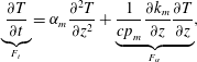 $$\begin{eqnarray}\displaystyle \underbrace{\frac{\unicode[STIX]{x2202}T}{\unicode[STIX]{x2202}t}}_{F_{t}}=\unicode[STIX]{x1D6FC}_{m}\frac{\unicode[STIX]{x2202}^{2}T}{\unicode[STIX]{x2202}z^{2}}+\underbrace{\frac{1}{cp_{m}}\frac{\unicode[STIX]{x2202}k_{m}}{\unicode[STIX]{x2202}z}\frac{\unicode[STIX]{x2202}T}{\unicode[STIX]{x2202}z}}_{F_{\unicode[STIX]{x1D6FC}}}, & & \displaystyle\end{eqnarray}$$
where
 $\unicode[STIX]{x1D6FC}_{m}=k_{m}/cp_{m}$
is the thermal diffusivity. All of the temperature derivatives are calculated from the experimental data
 $T(z,t)$
as follows. We apply the first-order forward scheme to calculate the first derivative of
 $T(z,t)$
. A cubic smoothing spline is used to filter out the noise in
 $\unicode[STIX]{x2202}T/\unicode[STIX]{x2202}z$
due to local temperature fluctuations. Then the first-order backward scheme is applied to the results of
 $\unicode[STIX]{x2202}T/\unicode[STIX]{x2202}z$
to evaluate the second-order derivative
 $\unicode[STIX]{x2202}^{2}T/\unicode[STIX]{x2202}z^{2}$
. The thermal diffusivity
 $\unicode[STIX]{x1D6FC}_{m}$
, specific heat
 $cp_{m}$
and thermal conductivity
 $k_{m}$
are functions of the solid fraction
 $\unicode[STIX]{x1D719}$
, and thus (4.2) reduces to an equation that can be solved for
 $\unicode[STIX]{x1D719}$
at each height
 $z$
.
(a–c) Results for
 $\unicode[STIX]{x2202}T/\unicode[STIX]{x2202}t$
,
 $\unicode[STIX]{x2202}^{2}T/\unicode[STIX]{x2202}z^{2}$
and
 $\unicode[STIX]{x2202}T/\unicode[STIX]{x2202}z$
as a function of time measured during the sixth modulation period at
 $z=12~\text{mm}$
. (d) Phases for
 $\unicode[STIX]{x2202}T/\unicode[STIX]{x2202}t$
,
 $\unicode[STIX]{x2202}^{2}T/\unicode[STIX]{x2202}z^{2}$
and
 $\unicode[STIX]{x2202}T/\unicode[STIX]{x2202}z$
measured at different heights. Results for an initial concentration
 $C_{0}=29~\text{wt}\%$
,
 $A=10~\text{K}$
and
 $\unicode[STIX]{x1D70F}=4000~\text{s}$
.
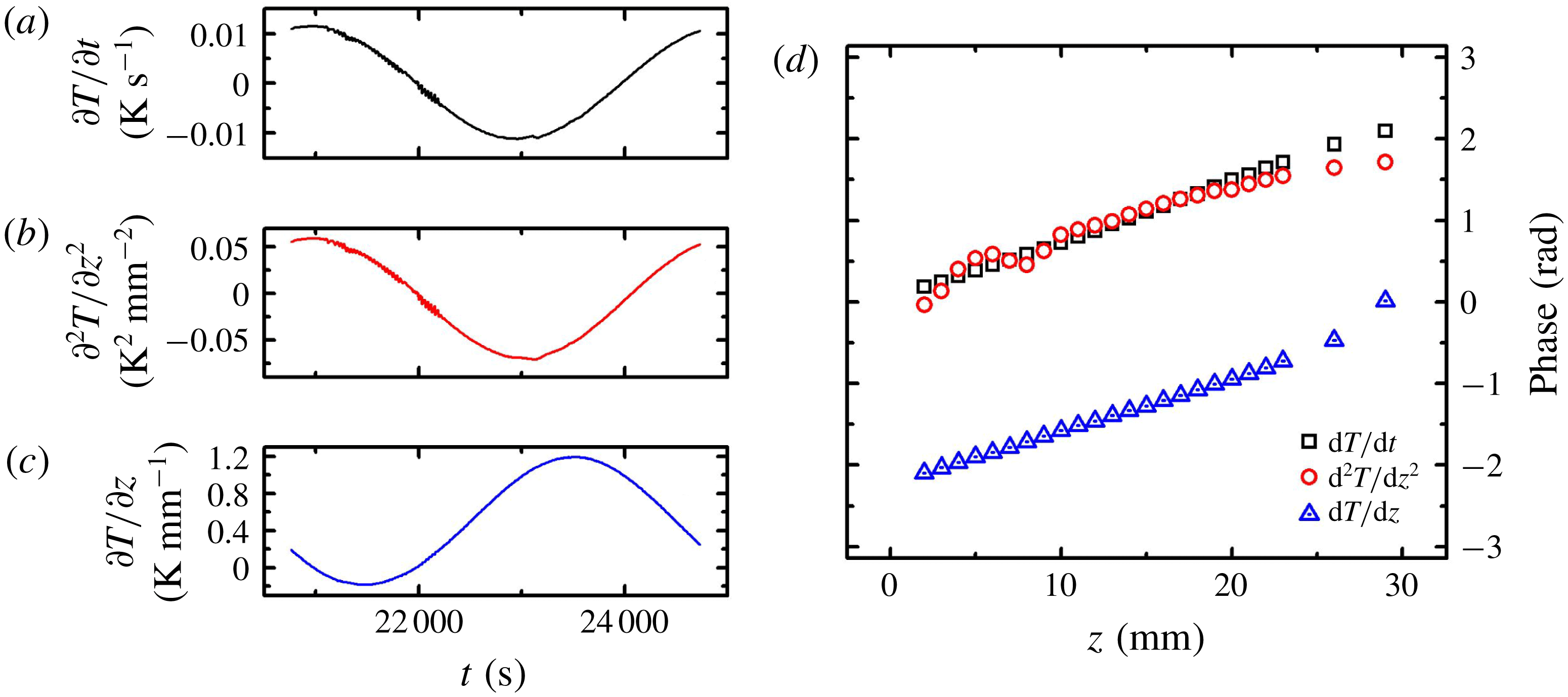
We examine the temporal properties of each term in equation (4.2). Figure 7 presents
 $\unicode[STIX]{x2202}T/\unicode[STIX]{x2202}t$
,
 $\unicode[STIX]{x2202}^{2}T/\unicode[STIX]{x2202}z^{2}$
and
 $\unicode[STIX]{x2202}T/\unicode[STIX]{x2202}z$
as functions of time at a given height
 $z=12~\text{mm}$
. We see that both the temporal and spatial derivatives vary periodically in time in response to the modulation of
 $T_{b}$
. If one assumes that
 $\unicode[STIX]{x1D719}$
and hence the material properties evolve much slower than the rapid variations of temperature, then the phases of
 $F_{T}$
and
 $F_{\unicode[STIX]{x1D6FC}}$
are given by the phases of
 $\unicode[STIX]{x2202}T/\unicode[STIX]{x2202}t$
and
 $\unicode[STIX]{x2202}T/\unicode[STIX]{x2202}z$
, respectively. Moreover, the phases of both sides of equation (4.2) must be the same.
A first glance at figure 7 suggests that the phases of
 $\unicode[STIX]{x2202}^{2}T/\unicode[STIX]{x2202}z^{2}$
and
 $\unicode[STIX]{x2202}T/\unicode[STIX]{x2202}t$
are close to each other. Thus the magnitude of
 $F_{\unicode[STIX]{x1D6FC}}$
should be relatively small. However, closer inspection of the data reveals that there are still slight phase differences between
 $\unicode[STIX]{x2202}^{2}T/\unicode[STIX]{x2202}z^{2}$
and
 $\unicode[STIX]{x2202}T/\unicode[STIX]{x2202}t$
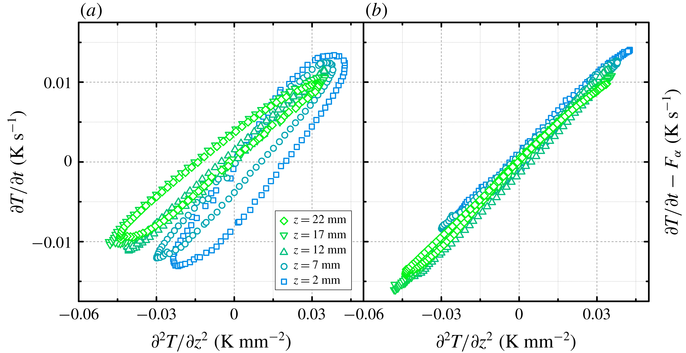
. Figure 8(a) shows
 $\unicode[STIX]{x2202}^{2}T/\unicode[STIX]{x2202}z^{2}$
against
 $\unicode[STIX]{x2202}T/\unicode[STIX]{x2202}t$
measured at different heights. If
 $\unicode[STIX]{x2202}^{2}T/\unicode[STIX]{x2202}z^{2}$
and
 $\unicode[STIX]{x2202}T/\unicode[STIX]{x2202}t$
have the same phase, then data points in the figure should collapse into a straight line with
 $\unicode[STIX]{x2202}T/\unicode[STIX]{x2202}t\propto \unicode[STIX]{x2202}^{2}T/\unicode[STIX]{x2202}z^{2}$
. However, one can see that the data points in fact constitute a curve with the shape of a tilted ellipse, indicating there is a non-trivial difference in phase between
 $F_{T}$
and
 $F_{\unicode[STIX]{x1D6FC}}$
and thus the first-derivative term
 $F_{\unicode[STIX]{x1D6FC}}$
is non-negligible.
To account for the effect of the periodically varying mush temperature and the fact that
 $F_{T}$
dominates the conductive heat transport, we adopt a mathematical scheme to resolve
 $\unicode[STIX]{x1D6FC}_{m}$
from the heat equation. We rewrite (4.2) in the following form:
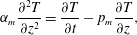 $$\begin{eqnarray}\displaystyle \unicode[STIX]{x1D6FC}_{m}\frac{\unicode[STIX]{x2202}^{2}T}{\unicode[STIX]{x2202}z^{2}}=\frac{\unicode[STIX]{x2202}T}{\unicode[STIX]{x2202}t}-p_{m}\frac{\unicode[STIX]{x2202}T}{\unicode[STIX]{x2202}z}, & & \displaystyle\end{eqnarray}$$
where
 $p_{m}=1/cp_{m}(\unicode[STIX]{x2202}k_{m}/\unicode[STIX]{x2202}z)$
. We first determine
 $p_{m}$
at each depth, using the fact that the phase of
 $\unicode[STIX]{x2202}T/\unicode[STIX]{x2202}t-p_{m}\unicode[STIX]{x2202}T/\unicode[STIX]{x2202}z$
should be identical to that of
 $\unicode[STIX]{x2202}^{2}T/\unicode[STIX]{x2202}z^{2}$
. The calculation of
 $p_{m}$
is achieved through a shooting scheme, with the value of
 $p_{m}$
initially given and adjusted according to the phase difference between
 $\unicode[STIX]{x2202}T/\unicode[STIX]{x2202}t-p_{m}\unicode[STIX]{x2202}T/\unicode[STIX]{x2202}z$
and
 $\unicode[STIX]{x2202}^{2}T/\unicode[STIX]{x2202}z^{2}$
. Having determined
 $p_{m}$
, we then solve for the thermal diffusivity
 $\unicode[STIX]{x1D6FC}_{m}$
given by the constraint that the magnitudes of both sides in (4.2) have to be the same. With
 $p_{m}$
determined through this scheme, we plot
 $\unicode[STIX]{x2202}T/\unicode[STIX]{x2202}t-F_{\unicode[STIX]{x1D6FC}}$
as a function of
 $\unicode[STIX]{x2202}^{2}T/\unicode[STIX]{x2202}z^{2}$
in figure 8(b). Data points in figure 8(b) collapse into straight lines crossing the origin. The thermal diffusivity
 $\unicode[STIX]{x1D6FC}_{m}$
is then determined by linear fitting of the data using a least-squares method. We find results of
 $\unicode[STIX]{x1D6FC}_{m}(z)$
are nearly independent of the modulation period, thus validating the assumption that
 $\unicode[STIX]{x1D719}$
has no long-term trend over time and is insensitive to the rapid variations of temperature (see also results in figure 10). Profiles of the solid fraction
 $\unicode[STIX]{x1D719}$
are finally determined from
 $\unicode[STIX]{x1D6FC}_{m}(z)=k_{m}/cp_{m}$
, where
 $k_{m}$
and
 $cp_{m}$
are expressed in terms of
 $\unicode[STIX]{x1D719}$
using the physical parameters shown in table 1. Note that the collapse seen in figure 8(b) shows some similarities to the method used by Pringle et al. (Reference Pringle, Eicken, Trodahl and Backstrom2007) to determine the thermal conductivity of sea ice from a fit of
 $k_{m}\unicode[STIX]{x2202}^{2}T/\unicode[STIX]{x2202}z^{2}$
versus
 $\unicode[STIX]{x1D70C}\unicode[STIX]{x2202}U/\unicode[STIX]{x2202}t-(\unicode[STIX]{x2202}k_{m}/\unicode[STIX]{x2202}z)(\unicode[STIX]{x2202}T/\unicode[STIX]{x2202}z)$
, where
 $U$
is the sea-ice internal energy per unit mass and
 $\unicode[STIX]{x1D70C}$
the density. However, in order to determine the internal energy the approach of Pringle et al. (Reference Pringle, Eicken, Trodahl and Backstrom2007) used independent measurements of bulk concentration as a function of depth from sea-ice cores along with the temperature, whilst we infer
 $\unicode[STIX]{x1D719}$
without independent knowledge of the bulk concentration.
Heat-flux diagrams: (a)
 $\unicode[STIX]{x2202}T/\unicode[STIX]{x2202}t$
as a function of
 $\unicode[STIX]{x2202}^{2}T/\unicode[STIX]{x2202}z^{2}$
and (b)
 $\unicode[STIX]{x2202}T/\unicode[STIX]{x2202}t-F_{\unicode[STIX]{x1D6FC}}$
as a function of
 $\unicode[STIX]{x2202}^{2}T/\unicode[STIX]{x2202}z^{2}$
. Results for an initial concentration
 $C_{0}=29~\text{wt}\%$
,
 $A=10~\text{K}$
and
 $\unicode[STIX]{x1D70F}=4000~\text{s}$
.
The parameter values used in calculation (Peppin, Huppert & Worster Reference Peppin, Huppert and Worster2008).

In our numerical scheme
 $\unicode[STIX]{x1D6FC}_{m}$
and
 $p_{m}$
are determined independently, based on the equalities of the phases and magnitudes on both sides of (4.3). Since
 $$\begin{eqnarray}\displaystyle p_{m}(z)=\frac{1}{cp_{m}}\frac{\unicode[STIX]{x2202}k_{m}}{\unicode[STIX]{x2202}z}=\frac{k_{s}-k_{l}}{cp_{s}\unicode[STIX]{x1D719}+cp_{l}(1-\unicode[STIX]{x1D719})}\frac{\text{d}\unicode[STIX]{x1D719}}{\text{d}z}, & & \displaystyle\end{eqnarray}$$
a second estimate of the solid fraction, represented by
 $\unicode[STIX]{x1D719}_{p}(z)$
, can be obtained given by the profiles of
 $p_{m}(z)$
. We solved (4.4) using a fourth-order Runge–Kutta method, integrating from the mush–liquid interface to the bottom. To reduce the error caused by the difference of height between the thermistors and the mush–liquid interface, we have employed a shooting method scheme, with the initial solid fraction
 $\unicode[STIX]{x1D719}_{i}$
(at the uppermost thermistor in the mush) adjusted to minimize the difference between
 $\overline{\unicode[STIX]{x1D719}_{p}}$
and
 $\overline{\unicode[STIX]{x1D719}}$
. Comparing
 $\unicode[STIX]{x1D719}_{p}$
with
 $\unicode[STIX]{x1D719}$
provides a consistency check on the method.
4.3 Distributions of solid fraction in mushy layers with various initial concentrations
Profiles of
 $\unicode[STIX]{x1D719}(z)$
for different initial concentrations. (a) The solid fraction
 $\unicode[STIX]{x1D719}$
as a function of height
 $z$
within the mushy layer. (b) The solid fraction
 $\unicode[STIX]{x1D719}$
as a function of the normalized height
 $z^{\ast }=z/h$
. The error bars indicate the difference between
 $\unicode[STIX]{x1D719}$
and
 $\unicode[STIX]{x1D719}_{p}$
determined from (4.4). Inset in (a): a comparison of
 $\unicode[STIX]{x1D719}$
(solid line) and
 $\unicode[STIX]{x1D719}_{p}$
(dashed line) obtained from the separate approaches. Measurements are taken in the sixth modulation period with
 $A=10~\text{K}$
and
 $\unicode[STIX]{x1D70F}=4000~\text{s}$
.
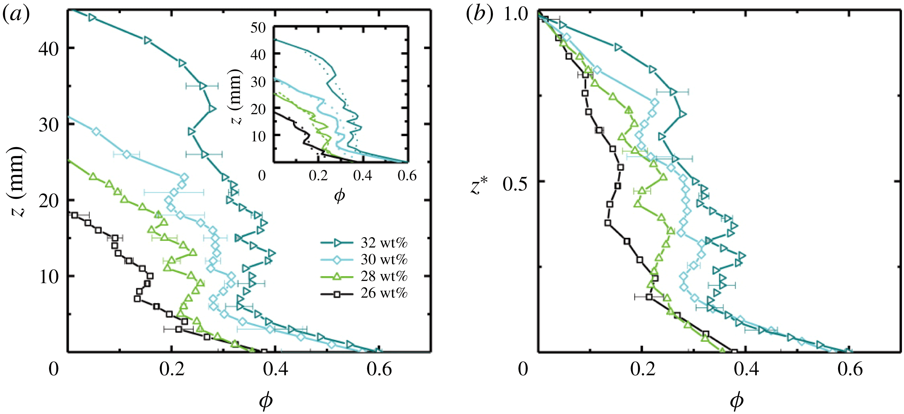
Figure 9(a) presents results of solid-fraction profiles
 $\unicode[STIX]{x1D719}(z)$
for different initial concentration
 $C_{0}$
. The mushy-layer height as well as the mean solid fraction
 $\bar{\unicode[STIX]{x1D719}}$
appear to increase as
 $C_{0}$
increases. The general features of the profiles
 $\unicode[STIX]{x1D719}(z)$
also depend on
 $C_{0}$
. For a high initial concentration
 $C_{0}$
, the solid fraction
 $\unicode[STIX]{x1D719}(z)$
exhibits a cliff–ramp–cliff structure: near the bottom and interface
 $\unicode[STIX]{x1D719}(z)$
decreases rapidly as
 $z$
increases; but in the bulk of the mushy layer,
 $\unicode[STIX]{x1D719}(z)$
varies relatively slowly with
 $z$
. The cliff–ramp–cliff structure is more pronounced for higher
 $C_{0}$
. Larger local fluctuations of
 $\unicode[STIX]{x1D719}$
with height are also seen for higher
 $C_{0}$
. These results suggest that as the mushy layer thickness increases for higher initial concentration, the internal dendritic structure of the mushy layer becomes more complex and varies more erratically in space. On the other hand, for low
 $C_{0}$
the solid fraction
 $\unicode[STIX]{x1D719}(z)$
decreases almost linearly with
 $z$
with smaller fluctuations at each height, indicating the dendritic structure of the mushy layer is relatively simple. The dependence of the solid fraction profiles on the initial concentration is further demonstrated in figure 9(b), where we show
 $\unicode[STIX]{x1D719}$
as a function of the normalized height
 $z^{\ast }=z/h$
. We speculate that such variability in
 $\unicode[STIX]{x1D719}$
might result from prior local solute fluxes caused by gravity drainage, although this is not conclusively demonstrated here. In the inset of figure 9(a), we compare results of
 $\unicode[STIX]{x1D719}(z)$
and
 $\unicode[STIX]{x1D719}_{p}(z)$
that were derived from
 $\unicode[STIX]{x1D6FC}_{m}(z)$
and
 $p_{m}(z)$
. The spatial fluctuation of
 $\unicode[STIX]{x1D719}$
is in general larger than that of
 $\unicode[STIX]{x1D719}_{p}$
. Fluctuations are likely smoothed by the method used to determine
 $\unicode[STIX]{x1D719}_{p}$
, because the process of numerical integration acts as a natural smoothing filter for high-frequency fluctuations. Beyond the fluctuations, the patterns of depth dependence of
 $\unicode[STIX]{x1D719}$
and
 $\unicode[STIX]{x1D719}_{p}$
are mainly consistent. The deviation of
 $\unicode[STIX]{x1D719}_{p}$
from
 $\unicode[STIX]{x1D719}$
is greater when
 $C_{0}$
increases, indicating the greater spatial variance of the mushy-layer structure for higher
 $C_{0}$
.
Profiles of
 $\unicode[STIX]{x1D719}(z)$
measured at different modulation periods. Results for (a)
 $C_{0}=29.0~\text{wt}\%$
and (b)
 $C_{0}=32.0~\text{wt}\%$
with
 $A=10~\text{K}$
and
 $\unicode[STIX]{x1D70F}=4000~\text{s}$
. The error bars indicate the difference between
 $\unicode[STIX]{x1D719}$
and
 $\unicode[STIX]{x1D719}_{p}$
determined from (4.4).
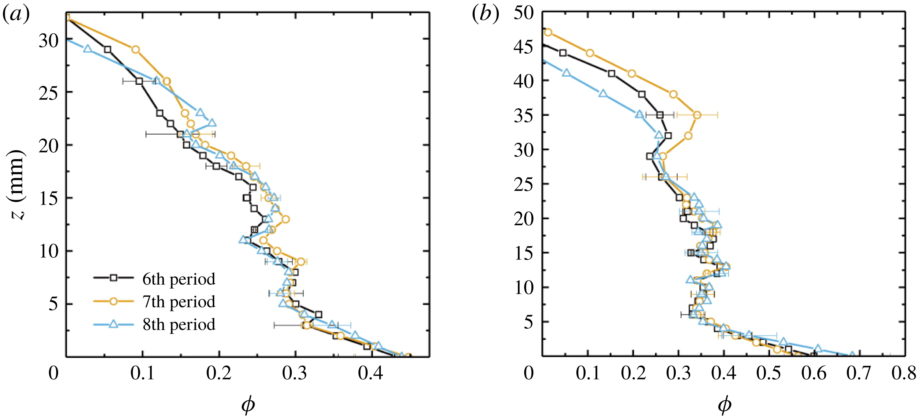
In figure 10 we compare results of
 $\unicode[STIX]{x1D719}(z)$
measured at different modulation periods (
 $t=6\unicode[STIX]{x1D70F}$
,
 $7\unicode[STIX]{x1D70F}$
and
 $8\unicode[STIX]{x1D70F}$
) with two initial concentrations
 $C_{0}=29.0$
and 32.0 wt%. The error bar represents the difference between
 $\unicode[STIX]{x1D719}$
and
 $\unicode[STIX]{x1D719}_{p}$
. We see that the solid fraction
 $\unicode[STIX]{x1D719}(z)$
becomes approximately independent of time throughout much of the depth in these late modulation periods, as the three profiles nearly overlap with each other (the other experiments not shown in figure 10 also have a similar level of time-independence of
 $\unicode[STIX]{x1D719}(z)$
for
 $t\geqslant 7\unicode[STIX]{x1D70F}$
). Their consistency is better near the cooling boundary than close to the mush–liquid interface. These results suggest that, in the late-time period, growth of the mushy layer is already in the asymptotic state in which both thickness and the dendritic structure of the mushy layer show only a weak long-term temporal trend. Whilst there may be some fluxes of comparatively fresh water from selected chimneys which may cause some change in bulk concentration and drift in the solid fraction, we conclude that the resulting changes to
 $\unicode[STIX]{x1D719}$
are small in the interior of the mushy layer over this time scale (sixth to eighth modulation periods). It is possible that the slight retreat of the mean position of the mush–liquid interface (as seen in figure 2
d) is linked to the greater variation in
 $\unicode[STIX]{x1D719}$
seen near the mush–liquid interface. However, the fluid advection and the turbulent heat transport are notable close to the mush–liquid interface, and may give rise to large temperature fluctuations there. Hence our measurements of
 $\unicode[STIX]{x1D719}(z)$
based on the local fluid temperature data may be less repeatable very close to the mush–liquid interface. It is worth noting that results for the local fluctuations of
 $\unicode[STIX]{x1D719}(z)$
in the mid-height region (
 $5~\text{mm}\leqslant z\leqslant 20~\text{mm}$
) are in close agreement in the three runs. Thus they may reveal the fine structures in the solid fraction profiles: there are large excursions of the mush porosity along the vertical profiles when growing with high initial concentrations.
The cliff–ramp–cliff structure of
 $\unicode[STIX]{x1D719}(z)$
measured here was also observed by Chen (Reference Chen1995) through computed tomography, and by Aussillous et al. (Reference Aussillous, Sederman, Gladden, Huppert and Worster2006) using magnetic resonance imaging. It seems not to agree with the measurements of Shirtcliffe et al. (Reference Shirtcliffe, Huppert and Worster1991) and Worster (Reference Worster1992). The reason for this disagreement may be that the present study measured at late times where the dendritic structure of the mushy layer was nearly independent of time. However, measurements of Shirtcliffe et al. (Reference Shirtcliffe, Huppert and Worster1991) and Worster (Reference Worster1992) were performed in an early period when the growth and development of the dendritic structure in the mushy layer are significant. The accumulated effects of solute diffusion grow over time, and hence it is possible that the observed basal ramp feature may be a result of solute transport. Because of the coupling of temperature and concentration by the liquidus relation, the thermal gradient at the cold lower boundary leads to a corresponding solute gradient. Thus solutal diffusion transports solute towards the boundary. Unlike heat, solute cannot be removed through the lower boundary, and hence builds up over time, with a tendency towards local supersaturation of
 $\text{NH}_{4}\text{Cl}$
that is relieved by enhanced solidification in a diffusive boundary layer near to the base. Using a solutal diffusivity
 $D_{s}=1.3\times 10^{-3}~\text{mm}^{2}~\text{s}^{-1}$
(Neufeld & Wettlaufer Reference Neufeld and Wettlaufer2008) the diffusion length after 24 000 s is
 $\sqrt{D_{s}t}\approx 6~\text{mm}$
. This is commensurate with the basal boundary-layer thickness in figure 10 after six modulation periods, lending further support to the hypothesized role of solute diffusion.
4.4 The mean solid fractions measured in the mush and liquid region
Vertical temperature (a) and concentration (b) profiles measured in the liquid region in the middle of the sixth modulation period with
 $A=10~\text{K}$
and
 $\unicode[STIX]{x1D70F}=4000~\text{s}$
. Blue curve:
 $C_{0}=26~\text{wt}\%$
; green curve:
 $C_{0}=29~\text{wt}\%$
; red curve:
 $C_{0}=30~\text{wt}\%$
. Positions of the inflection points (where the vertical gradient is maximum) along the curves
 $C(z)$
in (b) coincide with the top and bottom interfaces of the double-diffusive layers indicated by pairs of horizontal dashed lines for
 $C_{0}=29~\text{wt}\%$
.
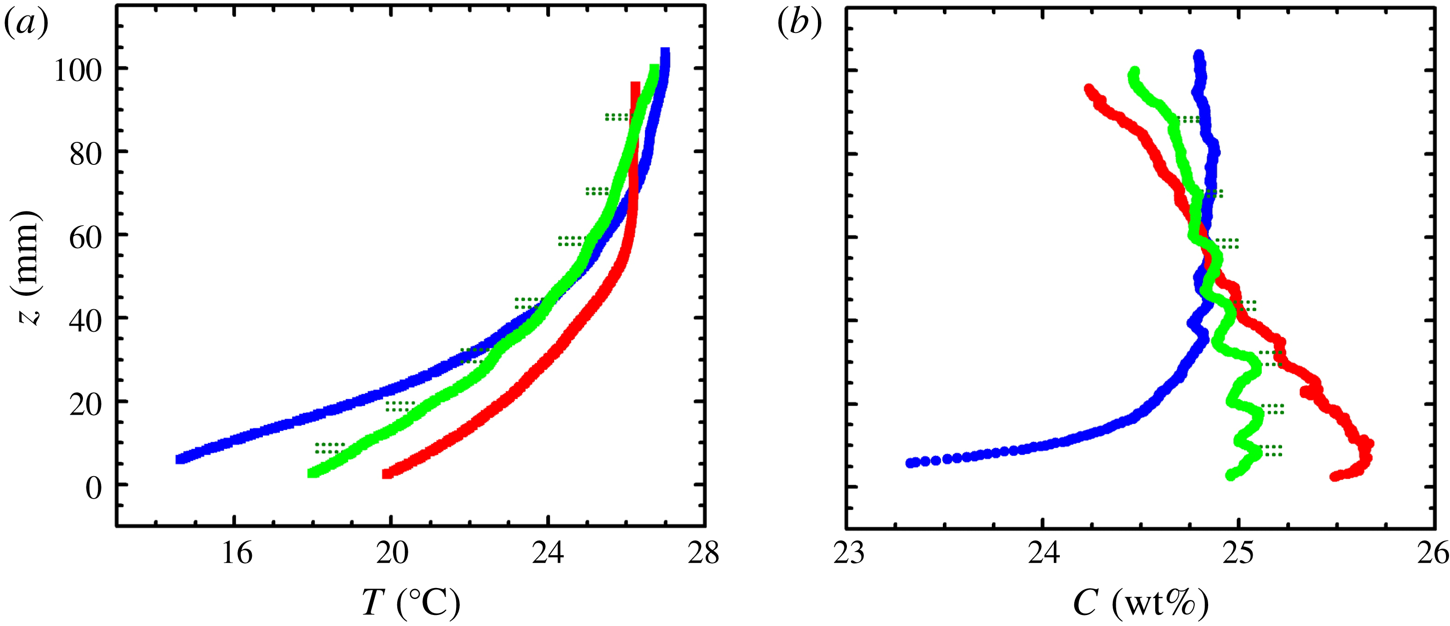
We also performed measurements of the concentration and temperature distributions in the liquid region during the experiment. Profiles of
 $C(z)$
and
 $T(z)$
were collected by a conductivity–temperature probe traversing vertically across the liquid region (see § 2 and figure 1
a). Figure 11(a) shows three sets of temperature profiles
 $T(z)$
for initial fluid concentrations
 $C_{0}=26$
, 29 and 30 wt%, respectively. There is a sharp statically stable temperature gradient in the near field above the mushy layer and overall an increasing mean temperature as the height increases. With a larger
 $C_{0}$
we observed a smaller temperature gradient just above the mushy layer due to the higher interfacial temperature. Moreover, the temperature field becomes more uniform in the far field near the top boundary of the liquid region. Further examinations of these temperature profiles reveal several sharp changes of the temperature gradient with
 $z$
, for large
 $C_{0}$
. Such fine structures are superimposed on the background of a large temperature gradient in the near field, most clearly seen with
 $C_{0}=29~\text{wt}\%$
. We ascribe the formation of these structures to double-diffusive convection that enhances local thermal mixing of the fluid within each convection cell (figure 1
a), as discussed below.
Driven by the mushy-layer mode convection, relatively low-density fluid was continuously transported by plumes from chimneys in the mushy region, upwards through the overlying liquid region (figure 1
a). By the late modulation periods, a stable compositional stratification is established in the liquid region, and we observed the formation of double-diffusive layers with a horizontal temperature gradient created by the cold chimney plumes. (The formation of the double-diffusive layers is through flow intrusions in the stratified background fluid driven by the horizontal thermal gradient; see discussions in Thorpe, Hutt & Soulsby (Reference Thorpe, Hutt and Soulsby1969), Jeevaraj & Imberger (Reference Jeevaraj and Imberger1991) and Wettlaufer et al. (Reference Wettlaufer, Worster and Huppert1997).) The signature of these double-diffusive layers is more pronounced in the concentration profiles
 $C(z)$
shown in figure 11(b). We find that the vertical positions of
 $C(z)$
with the sharpest gradient coincide with those of the double-diffusive layer interfaces indicated by pairs of horizontal dashed lines (see the supplementary materials in Part 1 for movies that capture the evolution of the double-diffusive layers in a state with background convection of the liquid region above a growing mushy layer, in both constant cooling and periodic cooling modes).
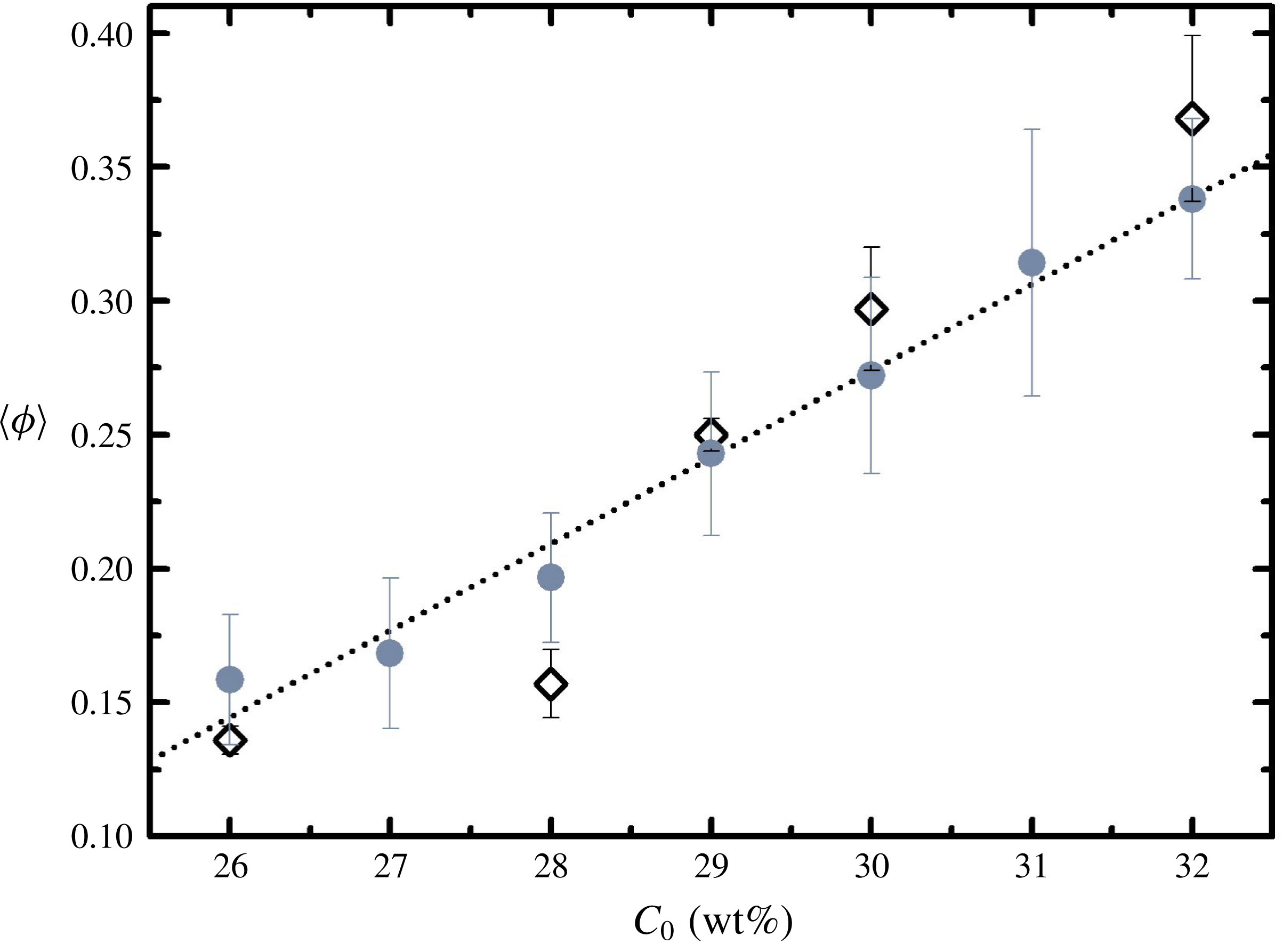
The depth-mean solid fraction in the mushy layer plotted as a function of the initial liquid concentration
 $C_{0}$
. Results
 $\overline{\unicode[STIX]{x1D719}}$
are obtained from temperature data analysis (filled circles) and
 $\langle \unicode[STIX]{x1D719}\rangle$
from direct concentration measurements in the liquid region (open diamonds). The error bars indicate the standard deviation of
 $\unicode[STIX]{x1D719}_{p}-\unicode[STIX]{x1D719}$
for temperature data analysis
 $\overline{\unicode[STIX]{x1D719}}$
, and maximum difference between measurements for the concentration method
 $\langle \unicode[STIX]{x1D719}\rangle$
. The dotted straight line shows a linear regression
 $\overline{\unicode[STIX]{x1D719}}=0.0323C_{0}-0.7$
.
The results of
 $T(z)$
and
 $C(z)$
shown in figure 11 enable us to independently determine the mean solid fraction in the mushy layer. Assuming local thermodynamic equilibrium is reached in the mushy layer with
 $T=T_{L}(C)=T_{E}+\unicode[STIX]{x1D6E4}(C-C_{E})$
, then applying solute conservation to the entire depth of the tank yields
 $$\begin{eqnarray}\displaystyle h\langle \unicode[STIX]{x1D719}\rangle +(1-\langle \unicode[STIX]{x1D719}\rangle )\int _{0}^{h}\left(\frac{T-T_{E}}{\unicode[STIX]{x1D6E4}}+C_{E}\right)\text{d}z+\int _{h}^{H}C(z)\,\text{d}z=C_{0}H, & & \displaystyle\end{eqnarray}$$
where
 $H$
is the height of the tank, the solid concentration
 $C_{s}=1$
and
 $\langle \unicode[STIX]{x1D719}\rangle$
is the average solid fraction weighted by the total concentration over the mushy layer. Formally,
 $\langle \unicode[STIX]{x1D719}\rangle$
is defined by
 $C_{s}\langle \unicode[STIX]{x1D719}\rangle +\overline{C}(1-\langle \unicode[STIX]{x1D719}\rangle )=\overline{C_{s}\unicode[STIX]{x1D719}+C(1-\unicode[STIX]{x1D719})}$
, where overbars denote a vertical average over the mushy region. For each initial concentration
 $C_{0}$
we have made measurements of
 $C(z)$
by scanning the probe over the entire depth of the liquid region several times during the sixth modulation period, Results of the averaged
 $C(z)$
are used to determine
 $\langle \unicode[STIX]{x1D719}\rangle$
through (4.5).
Meanwhile we determine the mean depth-averaged solid fraction
 $\overline{\unicode[STIX]{x1D719}}$
by depth-integrating profiles of
 $\unicode[STIX]{x1D719}(z)$
that were obtained from the thermal response of the mushy layer (figure 9). Results for
 $\langle \unicode[STIX]{x1D719}\rangle$
and
 $\overline{\unicode[STIX]{x1D719}}$
obtained in both methods are shown as a function of the initial concentration
 $C_{0}$
in figure 12. We find that for low
 $C_{0}$
the mean solid fraction
 $\overline{\unicode[STIX]{x1D719}}$
is slightly overestimated in the temperature-measurement approach, possibly because a relatively lower resolution for
 $\unicode[STIX]{x1D719}(z)$
was obtained in thinner mushy layers. With high initial concentration
 $C_{0}$
, there is better agreement of
 $\overline{\unicode[STIX]{x1D719}}$
and
 $\langle \unicode[STIX]{x1D719}\rangle$
. Overall, the good agreement of the two sets of data obtained from independent experimental approaches indicates that our method of temperature-data analysis is adequate to provide relatively accurate results for the mean solid-fraction distribution in a mushy layer.
5 Summary and discussion
This paper presents experimental studies of the distributions of temperature and solid fraction of growing mushy layers that are subjected to periodical cooling from below. A new method is presented for determining vertical profiles of solid fraction in the mushy layer based on high-resolution temperature measurements. Here we summarize the main results and discuss questions that are still open for future investigation.
The evolution of the local temperature
 $T(z,t)$
at various heights demonstrates that the temperature oscillations of the bottom boundary
 $T_{b}$
propagate through the mushy layer with substantial decay in the amplitude and phase delays. We find that the phase lag of
 $T(z,t)$
behind
 $T_{b}$
increases approximately linearly with increasing height, which indicates a constant propagation speed of the thermal oscillations. The oscillation amplitude of
 $T(z,t)$
decays exponentially in depth. Both features are consistent with the classical thermal wave behaviour for diffusive transport subject to a varying surface temperature. The decay rate decreases with an increasing initial concentration, but the propagation speed increases with increasing concentration. Comparing to the thermal wave problem, these observations suggest that a higher fluid concentration leads to a greater solid fraction on average, which enhances the thermal conductivity and reduces the specific heat in the mushy layer.
We compared the scaled vertical temperature profiles
 $T^{\ast }(z^{\ast })$
at different oscillation phases. The results show that a negative temperature gradient may appear near to the bottom boundary of the mush when the boundary temperature
 $T_{b}$
is close to minimum. We attribute this phenomenon to the finite propagation speed of the temperature oscillations through the mushy layer. This effect is more pronounced in late growth periods and with large initial concentrations, when a larger mush thickness reduces the average temperature gradient across the mushy layer. Experimental results during the late growth periods show that the temperature evolution within a modulation period is highly repeatable at each height near the bottom boundary (figure 2), indicating that the thermal properties and therefore the porosity structure of the mushy layer become nearly independent of time near
 $z=0$
. The conclusion is supported as well by direct solid-fraction measurements as shown in figure 10. However, near the mush–liquid interface we find
 $\unicode[STIX]{x1D719}(z)$
is still slightly drifting in time in this stage (figure 10). The small variations of
 $\unicode[STIX]{x1D719}(z)$
near
 $z=h$
may be due to the brine flux carried by the chimney plumes that still exist in late modulation periods as shown in figure 1(a), acting in concert with a slight retreat of the position of the mush–liquid interface as seen in figure 2(d).
Through measurements of temperature we determine the various components of heat transport through the mushy layer and reveal that neither the advection heat flux nor the latent heat transfer plays an important role in the heat equation at late times, when the mushy layer is oscillating about a nearly steady background state. The heat transport through conduction is the main component that determines the rate of change of the specific heat. Based on these experimental findings, we developed a mathematical scheme to solve for the depth dependence of the thermal conductivity and the specific heat coefficient, and hence determine the solid-fraction profiles in the mushy layer for various initial concentrations. The method uses the response to small-to-moderate amplitude modulation of the boundary temperature in order to infer the material properties. In this theoretical scheme we separately consider the amplitude and the phase of terms in the heat equation, and determine the thermal diffusivity
 $\unicode[STIX]{x1D6FC}_{m}$
from the amplitude and the associated variable
 $p_{m}=(\unicode[STIX]{x2202}k_{m}/\unicode[STIX]{x2202}z)/(cp)_{m}$
from the phase. Estimates of the solid fraction determined by these two approaches are in good agreement with each other. We note that this approach to determining
 $\unicode[STIX]{x1D719}$
relies on well-resolved measurements of periodic temperature oscillations in the mushy layer. Because the amplitude of the thermal waves decays with height, this means that the signal-to-noise ratio will likely decrease with height through the mush. Hence solid fraction estimates very close to the mush–liquid interface may be less reliable if the thermal wave amplitude becomes comparable to convective fluctuations in the overlying fluid. The decay length scale
 $\sqrt{2\unicode[STIX]{x1D6FC}_{m}/\unicode[STIX]{x1D714}}$
scales with the diffusion length over a modulation period, and hence modulation periods approaching the diffusion time
 $h^{2}/\unicode[STIX]{x1D6FC}_{m}$
across the full mushy-layer depth will give a larger signal for probing the structure near the mush–liquid interface. The analysis also relies on a relatively small heat transport via convection within the mushy layer, and a comparatively small change in
 $\unicode[STIX]{x1D719}$
over a modulation period due to macroscopic solute transport (such as via gravity drainage). Understanding the impact of modulated thermal forcing on the dynamics of gravity drainage remains an open question.
Our experimental results show that profiles of the solid fraction
 $\unicode[STIX]{x1D719}(z)$
exhibit a cliff–ramp–cliff structure with a rapid decrease in
 $\unicode[STIX]{x1D719}$
with increasing
 $z$
near the bottom and mush–liquid interface, but less variation in the interior of the mushy layer. This structure is more pronounced for higher initial concentration
 $C_{0}$
. For very low concentrations the solid fraction appears to be linearly dependent on height. The volume average of the solid fraction, and the local fluctuations in
 $\unicode[STIX]{x1D719}(z)$
both increase as
 $C_{0}$
increases. We suggest that the basal ramp structure of the solid-fraction profiles is possibly due to the diffusive transport of solute towards the bottom boundary. As a result of local thermodynamic equilibrium, the temperature gradient through the mush leads to an accompanying gradient in the liquid concentration which allows a diffusive solute flux which cannot be lost through the impermeable lower boundary. The increasing build-up of solute leads to local solidification and the increasing solid fraction near the bottom boundary.
Finally we performed measurements of the fluid concentration in the liquid region. Through the conservation law for salinity, these measurements provide an independent evaluation of the mean solid fraction of the mushy layer. The agreement between both sets of experimental results suggests the adequateness of the present temperature-measurement approach in probing variation of the thermal properties in mushy layers. The measurements of fluid concentration and temperature also reveal interesting structures, which are broadly consistent with double-diffusive features formed by the interaction of a stable solute stratification with lateral cooling by the cold solute-depleted plumes rising from the mushy layer. Whilst peripheral to this study, these features may present an interesting topic for future work.
The solid fraction
 $\unicode[STIX]{x1D719}$
, or porosity
 $1-\unicode[STIX]{x1D719}$
, of solidifying alloys can have an important control on the material properties of the mushy layer, including the phase-weighted thermal, electrical and mechanical properties, along with the permeability to fluid transport. The solid fraction
 $\unicode[STIX]{x1D719}(z)$
and liquid concentration
 $C(z)$
also control the bulk phase-weighted composition of alloys that are rapidly quenched in industrial solidification processes (Copley et al.
Reference Copley, Giamei, Johnson and Hornbecker1970). Hence, quantification of
 $\unicode[STIX]{x1D719}$
is relevant to a range of engineering, geophysical and geological settings (as discussed by Zhong et al.
Reference Zhong, Fragoso, Wells and Wettlaufer2012). The analysis presented in § 4 provides a potential methodology to infer the solid fraction
 $\unicode[STIX]{x1D719}$
in settings where the mushy layer is subject to small-amplitude modulations in thermal forcing, and temperature measurements are readily available. An interesting potential application is the growth and evolution of sea ice, which is a mushy layer of salty brine and ice (Feltham et al.
Reference Feltham, Untersteiner, Wettlaufer and Worster2006). In addition to the varying material properties, the evolving porosity controls biological habitats and chemical transport within the sea-ice pore space (Hunke et al.
Reference Hunke, Notz, Turner and Vancoppenolle2011). Furthermore, estimates of
 $\unicode[STIX]{x1D719}(z,t)$
and
 $T(z,t)$
can be combined with the assumption of local thermodynamic equilibrium to estimate bulk salinity and infer a record of past salt fluxes from sea ice into the ocean (Notz & Worster Reference Notz and Worster2008) which drive mixing in the polar oceans. Temperature measurements are frequently made via thermistor strings embedded within boreholes in the evolving ice (cf. Richter-Menge et al.
Reference Richter-Menge, Perovich, Elder, Claffey, Rigor and Ortmeyer2006; Jackson et al.
Reference Jackson, Wilkinson, Maksym, Meldrum, Beckers, Haas and Mackenzie2013) but non-destructive estimates of solid fraction are more challenging and less common. Sea ice is subject to fluctuating atmospheric and oceanic forcing on a variety of time scales (including a diurnal cycle in spring and summer, which is shorter than the seasonal evolution of sea-ice thickness). This may offer a potential pathway to infer the solid fraction of sea ice from the response to fluctuating thermal forcing (although further work is needed to disentangle the response to the broad range of frequencies usually experienced in environmental settings). We hope that the results here provide useful insight for developing measurements of the solid fraction of mushy layers, both in sea ice and other environmental and engineering settings.
Acknowledgements
This work was supported by the National Science Foundation of China through grant nos. 11572230 and 11772235, and NSFC/RGC Joint grant no. 11561161004. J.-Q.Z. acknowledges support from the Fundamental Research Funds for the Central Universities (grant nos. 22120180115 and 22120180280). G.-Y.D. was supported partially by NSFC/RGC Joint grant no. CUHK437/15. A.J.W. acknowledges European Union Award PCIG13-GA-2013-618610 SEA-ICE-CFD, and thanks the Isaac Newton Institute for Mathematical Sciences for hospitality during the programme Mathematics of Sea Ice Phenomena (EPSRC grant EP/K032208/1).
Appendix A. Neglect of latent heating
In this appendix, we estimate the likely magnitude of the error incurred by neglecting the latent heating term in the analysis of § 4. From (4.1), the heat equation yields
 $$\begin{eqnarray}\displaystyle cp_{m}\frac{\unicode[STIX]{x2202}T}{\unicode[STIX]{x2202}t}=\frac{\unicode[STIX]{x2202}}{\unicode[STIX]{x2202}z}\left(k_{m}\frac{\unicode[STIX]{x2202}T}{\unicode[STIX]{x2202}z}\right)+L\frac{\unicode[STIX]{x2202}\unicode[STIX]{x1D719}}{\unicode[STIX]{x2202}t}, & & \displaystyle\end{eqnarray}$$
where we have neglected convective heat transport
 $(w=0)$
following the analysis in § 4. Figure 10 suggests that
 $\unicode[STIX]{x1D719}$
varies little between modulation periods, so that
 $\unicode[STIX]{x1D719}(t)$
has no significant long-term trend (but could still vary periodically in time over a modulation period). We now estimate the contribution of periodic modulation of
 $\unicode[STIX]{x1D719}$
. In Part 1 (Ding et al.
Reference Ding, Wells and Zhong2019) we estimated
 $\unicode[STIX]{x2202}\unicode[STIX]{x1D719}/\unicode[STIX]{x2202}t$
from solute conservation, neglecting solute transport at early times before there is significant modification of the bulk concentration by gravity drainage. Motivated by the lack of trend in
 $\unicode[STIX]{x1D719}(t)$
in figure 10 between modulation periods, we again assume that solute transport is weak at late times, so that the bulk phase-weighted solute concentration
 $$\begin{eqnarray}\displaystyle C_{bulk}(z)=\unicode[STIX]{x1D719}C_{s}+(1-\unicode[STIX]{x1D719})C(z,t) & & \displaystyle\end{eqnarray}$$
is locally constant in time, at late times. In constructing this argument we allow for the possibility that the bulk concentration may vary with height with
 $C_{bulk}(z)<C_{0}$
, as a result of solute fluxes from gravity drainage at earlier times. The condition (A 2) rearranges to yield
 $$\begin{eqnarray}\displaystyle \unicode[STIX]{x1D719}=\frac{C_{bulk}-C_{L}(T)}{C_{S}-C_{L}(T)}=\frac{T_{L}(C_{bulk})-T}{T_{L}(C_{S})-T}, & & \displaystyle\end{eqnarray}$$
where
 $T=T_{L}(C)=T_{E}+\unicode[STIX]{x1D6E4}(C-C_{E})$
is the assumed linear liquidus relation in the mushy layer, with inverse
 $C=C_{L}(T)$
. Taking the derivative of (A 3) and using the chain rule yields
 $$\begin{eqnarray}\displaystyle \frac{\unicode[STIX]{x2202}\unicode[STIX]{x1D719}}{\unicode[STIX]{x2202}t}=\frac{\text{d}\unicode[STIX]{x1D719}}{\text{d}T}\frac{\unicode[STIX]{x2202}T}{\unicode[STIX]{x2202}t},\quad \text{with }\frac{\text{d}\unicode[STIX]{x1D719}}{\text{d}T}=\frac{\unicode[STIX]{x1D719}-1}{T_{L}(C_{s})-T}. & & \displaystyle\end{eqnarray}$$
Using (A 4) to eliminate
 $\unicode[STIX]{x2202}\unicode[STIX]{x1D719}/\unicode[STIX]{x2202}t$
from (A 1) results in a nonlinear diffusion equation for
 $T$
 $$\begin{eqnarray}\displaystyle cp_{eff}\frac{\unicode[STIX]{x2202}T}{\unicode[STIX]{x2202}t}=\frac{\unicode[STIX]{x2202}}{\unicode[STIX]{x2202}z}\left(k_{m}\frac{\unicode[STIX]{x2202}T}{\unicode[STIX]{x2202}z}\right),\quad \text{where }cp_{eff}=cp_{s}\unicode[STIX]{x1D719}+cp_{l}(1-\unicode[STIX]{x1D719})+\frac{L(1-\unicode[STIX]{x1D719})}{T_{L}(C_{s})-T} & & \displaystyle\end{eqnarray}$$
is an effective heat capacity. Thus the latent heating term provides an equivalent effect to modifying the liquid heat capacity by an additive factor
 $L/[T_{L}(C_{s})-T]$
. Using
 $L=0.428~\text{J}~\text{mm}^{-3}$
,
 $\unicode[STIX]{x1D6E4}=4.72\,^{\circ }\text{C}~\text{wt}\%^{-1}$
,
 $T_{E}=-15.4\,^{\circ }\text{C}$
,
 $C_{E}=19.7~\text{wt}\%$
and
 $C_{S}=100~\text{wt}\%$
(Neufeld & Wettlaufer Reference Neufeld and Wettlaufer2008), then an approximate temperature range of
 $-10\,^{\circ }\text{C}<T<20\,^{\circ }\text{C}$
within the mushy layer (see figure 2) results in
 $1.15\times 10^{-3}~\text{J}~\text{mm}^{-3}~\text{K}^{-1}<L/[T_{L}(C_{s})-T]<1.25\times 10^{-3}~\text{J}~\text{mm}^{-3}~\text{K}^{-1}$
. This corresponds to 30 %–34 % of the liquid specific heat
 $cp_{l}$
from table 1, so that setting
 $\unicode[STIX]{x2202}\unicode[STIX]{x1D719}/\unicode[STIX]{x2202}t=0$
has a similar effect to an order 30 % change in the liquid heat capacity. Propagating this error through the estimate of
 $\unicode[STIX]{x1D719}(z)$
from
 $\unicode[STIX]{x1D6FC}_{m}$
yields a potential underestimate of
 $\unicode[STIX]{x1D719}$
no larger than
 $\unicode[STIX]{x0394}\unicode[STIX]{x1D719}=0.1$
, which is comparable to the error bars in figure 9.
Appendix B. Thermal wave solution with constant material properties
In this appendix, we outline the derivation of a diffusive thermal wave behaviour arising from modulation of the boundary temperature. To yield an analytically tractable problem that captures the essence of the full system, we approximate
 $cp_{eff}$
and
 $k_{m}$
as constants in (A 5), and define a constant diffusivity
 $\unicode[STIX]{x1D6FC}=k_{m}/cp_{eff}$
. In contrast to the early-time behaviour considered in Part 1 (Ding et al.
Reference Ding, Wells and Zhong2019), we consider a late-time limit where the mushy layer oscillates about a steady state of thickness
 $h_{0}$
where conduction of heat through the mushy layer balances the heat flux
 $F_{T}$
from the overlying liquid. We further consider a limit with high-frequency modulation
 $\unicode[STIX]{x1D714}h_{0}^{2}/\unicode[STIX]{x1D6FC}\gg 1$
, so that the modulation period
 $\unicode[STIX]{x1D70F}=2\unicode[STIX]{x03C0}/\unicode[STIX]{x1D714}$
is much shorter than the diffusion time scale
 $h_{0}^{2}/\unicode[STIX]{x1D6FC}$
across the mushy-layer depth. To build insight into the impact of boundary modulation we use a perturbative approach, assuming the scaled modulation amplitude
 $\unicode[STIX]{x1D716}=A/\unicode[STIX]{x0394}T_{0}\ll 1$
, where
 $\unicode[STIX]{x0394}T_{0}=T_{L}(C_{i})-T_{b,0}$
is the temperature difference between the mush–liquid interface (with concentration
 $C_{i}$
) and the mean basal temperature
 $T_{b,0}$
. One can replace
 $T_{L}(C_{i})\approx T_{L}(C_{0})$
below with reasonable accuracy. The separation of scales is marginal since
 $0.18\leqslant \unicode[STIX]{x1D716}\leqslant 0.53$
for
 $5\,^{\circ }\text{C}\leqslant A\leqslant 15\,^{\circ }\text{C}$
and
 $\unicode[STIX]{x0394}T_{0}=28.5\,^{\circ }\text{C}$
, but we still find that the expansion provides useful insight.
With the assumed constant material properties, (A 5) yields
 $$\begin{eqnarray}\displaystyle \frac{\unicode[STIX]{x2202}T}{\unicode[STIX]{x2202}t}=\unicode[STIX]{x1D6FC}\frac{\unicode[STIX]{x2202}^{2}T}{\unicode[STIX]{x2202}z^{2}}, & & \displaystyle\end{eqnarray}$$
which is subject to boundary conditions
 $$\begin{eqnarray}\displaystyle T=T_{b,0}+\unicode[STIX]{x1D716}\unicode[STIX]{x0394}T_{0}\sin (\unicode[STIX]{x1D714}t+\unicode[STIX]{x1D719}_{0})\quad \text{at }z=0,\quad T=T_{b,0}+\unicode[STIX]{x0394}T_{0}\quad \text{at }z=h, & & \displaystyle\end{eqnarray}$$
and the Stefan condition
 $$\begin{eqnarray}\displaystyle {\mathcal{S}}\unicode[STIX]{x0394}T_{0}\frac{\text{d}h}{\text{d}t}=\left.\unicode[STIX]{x1D6FC}\frac{\unicode[STIX]{x2202}T}{\unicode[STIX]{x2202}z}\right|_{z=h}-\frac{F_{T}}{cp_{m}},\quad {\mathcal{S}}=\frac{cp_{l}[T_{l}-T_{L}(C_{l})]+L\unicode[STIX]{x1D719}_{i}}{cp_{eff}\unicode[STIX]{x0394}T_{0}}, & & \displaystyle\end{eqnarray}$$
where
 $T_{l}$
is the far-field temperature of the overlying liquid and
 $\unicode[STIX]{x1D719}_{i}$
the assumed interfacial solid fraction (cf. equations (3.4), (3.6) and (3.7) in Part 1, Ding et al.
Reference Ding, Wells and Zhong2019). Expanding
 $T=T_{0}+\unicode[STIX]{x1D716}T_{1}+\cdots \,$
and
 $h=h_{0}+\unicode[STIX]{x1D716}h_{1}+\cdots \,$
we find that the leading-order problem at
 $O(\unicode[STIX]{x1D716}^{0})$
is
 $$\begin{eqnarray}\displaystyle \frac{\unicode[STIX]{x2202}T_{0}}{\unicode[STIX]{x2202}t}=\unicode[STIX]{x1D6FC}\frac{\unicode[STIX]{x2202}^{2}T_{0}}{\unicode[STIX]{x2202}z^{2}},\quad T_{0}=T_{b,0}\quad \text{at }z=0,\quad T_{0}=T_{b,0}+\unicode[STIX]{x0394}T_{0}\quad \text{at }z=h_{0}. & & \displaystyle\end{eqnarray}$$
The long-time steady-state solution to (B 4) and (B 3) is
 $$\begin{eqnarray}\displaystyle T_{0}=T_{b,0}+\unicode[STIX]{x0394}T_{0}\frac{z}{h_{0}},\quad h_{0}=\frac{\unicode[STIX]{x1D6FC}cp_{eff}\unicode[STIX]{x0394}T_{0}}{F_{T}}, & & \displaystyle\end{eqnarray}$$
where the steady mush thickness
 $h_{0}$
is maintained by the balance between conduction and the heat flux
 $F_{T}$
in the liquid.
At
 $O(\unicode[STIX]{x1D716})$
, the linearized perturbations to (B 1) and (B 2) satisfy
 $$\begin{eqnarray}\displaystyle \frac{\unicode[STIX]{x2202}T_{1}}{\unicode[STIX]{x2202}t}=\unicode[STIX]{x1D6FC}\frac{\unicode[STIX]{x2202}^{2}T_{1}}{\unicode[STIX]{x2202}z^{2}},\quad T_{1}=\unicode[STIX]{x0394}T_{0}\sin (\unicode[STIX]{x1D714}t+\unicode[STIX]{x1D719}_{0})\quad \text{at }z=0,\quad T_{1}+h_{1}\frac{\unicode[STIX]{x2202}T_{0}}{\unicode[STIX]{x2202}z}=0\quad \text{at }z=h_{0}, & & \displaystyle \nonumber\\ \displaystyle & & \displaystyle\end{eqnarray}$$
with the linearized perturbation to (B 3) yielding
 $$\begin{eqnarray}\displaystyle \unicode[STIX]{x0394}T_{0}{\mathcal{S}}\frac{\text{d}h_{1}}{\text{d}t}=\left.\unicode[STIX]{x1D6FC}\frac{\unicode[STIX]{x2202}T_{1}}{\unicode[STIX]{x2202}z}\right|_{z=h_{0}}+h_{1}\left.\unicode[STIX]{x1D6FC}\frac{\unicode[STIX]{x2202}^{2}T_{0}}{\unicode[STIX]{x2202}z^{2}}\right|_{z=h_{0}}. & & \displaystyle\end{eqnarray}$$
Note that we have here Taylor-expanded functions of the form
 $f(h_{0}+\unicode[STIX]{x1D716}h_{1})=f(h_{0})+\unicode[STIX]{x1D716}h_{1}f^{\prime }(h_{0})+\cdots \,$
for
 $\unicode[STIX]{x1D716}\ll 1$
. We analyse the system (B 6)–(B 7) in the limit of high-frequency modulation
 $\unicode[STIX]{x1D714}h_{0}^{2}/\unicode[STIX]{x1D6FC}\gg 1$
. We solve using complex variable methods, setting
 $T_{1}=\text{Im}[\tilde{T}(z)\text{e}^{\text{i}\unicode[STIX]{x1D714}t+\text{i}\unicode[STIX]{x1D719}_{0}}]$
and
 $h_{1}=\text{Im}[\tilde{h}\text{e}^{\text{i}\unicode[STIX]{x1D714}t+\text{i}\unicode[STIX]{x1D719}_{0}}]$
for complex
 $\tilde{T}$
and
 $\tilde{h}$
. Substituting this ansatz into (B 7) and eliminating derivatives of
 $T_{0}$
using (B 5) one can show that
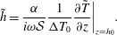 $$\begin{eqnarray}\displaystyle \tilde{h}=\frac{\unicode[STIX]{x1D6FC}}{i\unicode[STIX]{x1D714}{\mathcal{S}}}\frac{1}{\unicode[STIX]{x0394}T_{0}}\frac{\unicode[STIX]{x2202}\tilde{T}}{\unicode[STIX]{x2202}z}\bigg|_{z=h_{0}}. & & \displaystyle\end{eqnarray}$$
Hence (B 6) reduces to
 $$\begin{eqnarray}\displaystyle \frac{\text{i}\unicode[STIX]{x1D714}}{\unicode[STIX]{x1D6FC}}\tilde{T}=\frac{\unicode[STIX]{x2202}^{2}\tilde{T}}{\unicode[STIX]{x2202}z^{2}},\quad \frac{\tilde{T}}{\unicode[STIX]{x0394}T_{0}}=1\quad \text{at }z=0,\quad \frac{\tilde{T}}{\unicode[STIX]{x0394}T_{0}}=0+O\left(\frac{1}{{\mathcal{S}}}\frac{\unicode[STIX]{x1D6FC}}{\unicode[STIX]{x1D714}h_{0}^{2}}\right)\quad \text{at }z=h_{0},\qquad \quad & & \displaystyle\end{eqnarray}$$
where we again use (B 5) to eliminate
 $T_{0}$
.
Neglecting the terms of
 $O(\unicode[STIX]{x1D6FC}/\unicode[STIX]{x1D714}h_{0}^{2})$
, the solution to (B 9) is
 $$\begin{eqnarray}\displaystyle \frac{\tilde{T}}{\unicode[STIX]{x0394}T_{0}}=\frac{\text{e}^{-mz}-\text{e}^{-m(2h_{0}-z)}}{1-\text{e}^{-2mh_{0}}},\quad m=(1+i)\sqrt{\frac{\unicode[STIX]{x1D714}}{2\unicode[STIX]{x1D6FC}}}. & & \displaystyle\end{eqnarray}$$
This is easiest to interpret by exploiting the limit
 $|mh_{0}|=\sqrt{\unicode[STIX]{x1D714}h_{0}^{2}/\unicode[STIX]{x1D6FC}}\gg 1$
, from which we recover the classical thermal wave solution for diffusion in a deep layer with sinusoidally varying boundary temperature (e.g. see § 2.6 of Carslaw & Jaeger Reference Carslaw and Jaeger1959) with
 $\tilde{T}=\unicode[STIX]{x0394}T_{0}\text{e}^{-mz}$
and
 $$\begin{eqnarray}\displaystyle T=T_{0}(z,t)+A\text{e}^{-z\sqrt{\unicode[STIX]{x1D714}/2\unicode[STIX]{x1D6FC}}}\sin \left(\unicode[STIX]{x1D714}t-z\sqrt{\frac{\unicode[STIX]{x1D714}}{2\unicode[STIX]{x1D6FC}}}+\unicode[STIX]{x1D719}_{0}\right). & & \displaystyle\end{eqnarray}$$
The amplitude of the perturbation decays exponentially with e-folding length scale
 $\sqrt{2\unicode[STIX]{x1D6FC}/\unicode[STIX]{x1D714}}$
set by the approximate length scale for diffusion over a modulation cycle, whilst the phase
 $z\sqrt{\unicode[STIX]{x1D714}/2\unicode[STIX]{x1D6FC}}$
varies linearly with height over the same length scale, which recovers the internal thermal variation seen in figure 4.



