1 Introduction
Application areas such as intrusion detection, market basket analysis, and genomics and proteomics, to name just a few, generate millions of data points daily. A 2003 survey reports that the biggest decision support system at that time was at 29.2 terabytes, which is about 300% larger than the largest system in 2001 (Winter & Auerbach, Reference Winter and Auerbach2004). They also report that the average size of Unix databases experienced a 6-fold, and Windows databases a 14-fold, increase compared to year 2001, and that large commercial databases average about 10 billion data points (Winter & Auerbach, Reference Winter and Auerbach2004). This size explosion was triggered by recent advances in the low-cost storage technology and the growing interest of research and industrial communities in automated analysis of large quantities of data. Nowadays, data analysis algorithms, such as the classification algorithms, must scale with these increasing sizes.
Classification, that is, prediction of a class label of an unknown instance based on a classification model that is built from a set of training instances, is a methodology that is widely utilized in both academic and industrial settings. The instances are usually described by a set of features which can be nominal (e.g. color can be red, blue, white, etc.), ordinal (e.g. rank of a student in a class), and numerical including both interval and ratio scales (e.g. temperature or a height of a man). Both ordinal and numerical features are defined as continuous features, although ordinal features cannot be scaled, that is, we cannot judge how much better is a student ranked first when compared with a student who is ranked second or fifth. Some classification algorithms, like Naïve Bayes (NB; John & Langley, Reference John and Langley1995), AQ (Kaufman & Michalski, Reference Kaufman and Michalski1999), CLIP (Cios & Kurgan, Reference Cios and Kurgan2002, Reference Cios and Kurgan2004), CN2 (Clark & Niblett, Reference Clark and Niblett1989), and DataSqueezer (Kurgan et al., Reference Kurgan, Cios and Dick2006), work only with nominal features (and continuous features that take on a small number of values). Other classifiers that work with continuous features may perform better when dealing with nominal features (Rissanen, Reference Rissanen1978; Catlett, Reference Catlett1991; Liu et al., Reference Liu, Hussain, Tan and Dash2002; Kurgan & Cios, Reference Kurgan and Cios2004). Therefore, one of the important data preprocessing steps is discretization, which converts continuous features into discrete (nominal or ordinal) features. The key characteristic of discretization is that the number of values of a continuous feature is substantially reduced. The discretization methods were widely examined during the last two decades (Wong & Liu, Reference Wong and Liu1975; Rissanen, Reference Rissanen1978; Paterson & Niblett, Reference Paterson and Niblett1987; Wong & Chiu, Reference Wong and Chiu1987; Catlett, Reference Catlett1991; Kerber, Reference Kerber1992; Fayyad & Irani, Reference Fayyad and Irani1993; Ching et al., Reference Ching, Wong and Chan1995; Dougherty et al., Reference Dougherty, Kohavi and Sahami1995; Liu & Setiono, Reference Liu and Setiono1997; Wang & Liu, Reference Wang and Liu1998; Kurgan & Cios, Reference Kurgan and Cios2001; Tay & Shen, Reference Tay and Shen2002; Kurgan & Cios, Reference Kurgan and Cios2003; Boullé, Reference Boullé2004; Kurgan & Cios, Reference Kurgan and Cios2004; Liu & Wang, Reference Liu and Wang2005; Mehta et al., Reference Mehta, Parthasarathy and Yang2005; Boullé, Reference Boullé2006; Kujala & Elomaa, Reference Kujala and Elomaa2007; Lee, Reference Lee2007; Tsai et al., Reference Tsai, Lee and Yang2008). This research also addressed the impact of discretization on some of the classifiers such as decision trees including ID3 (Ching et al., Reference Ching, Wong and Chan1995), C4.5 (Fayyad & Irani, Reference Fayyad and Irani1992; Dougherty et al., Reference Dougherty, Kohavi and Sahami1995; Kohavi & Sahami, Reference Kohavi and Sahami1996; Liu & Setiono, Reference Liu and Setiono1997; Liu et al., Reference Liu, Hussain, Tan and Dash2002; Tay & Shen, Reference Tay and Shen2002; Liu & Wang, Reference Liu and Wang2005; Lee, Reference Lee2007), and C5.0 (Tay & Shen, Reference Tay and Shen2002; Kurgan & Cios, Reference Kurgan and Cios2003, Reference Kurgan and Cios2004; Tsai et al., Reference Tsai, Lee and Yang2008), AQ rule-based learners (Ching et al., Reference Ching, Wong and Chan1995), CLIP4 classifiers (Cios & Kurgan, Reference Cios and Kurgan2002; Kurgan & Cios, Reference Kurgan and Cios2003, Reference Kurgan and Cios2004), and nearest neighbor and logistic regression (Abraham et al., Reference Abraham, Simha and Iyengar2006).
As was shown in (Flores et al., Reference Flores, Inza and Larran2007), (Lee, Reference Lee2007), discretization has a positive impact on the NB classifier, that is, it helps to improve the classification performed with this classifier. This classifier is very easy to use, that is, it does not require the user to input any parameters, and provides competitive prediction accuracies (John & Langley, Reference John and Langley1995), (Webb et al., Reference Webb, Boughton and Wang2005; Zhang et al., Reference Zhang, Jiang and Su2005). NB was included in the recently published list of the top 10 data mining algorithms due to its simplicity, elegance, and robustness (Wu et al., Reference Wu, Kumar, Ross, Ghosh, Yang, Motoda, McLachlan, Ng, Liu, Yu, Zhou, Steinbach, Hand and Steinberg2007). One of the most attractive features of NB is that the classification model is built in linear time with respect to the number of instances, which allows for applications to large data sets. The above advantages lead to a number of follow-up studies that proposed novel extensions to the classical NB method (the so-called semi-NB classifiers; Langley et al., Reference Langley, Iba and Thompson1992; Langley & Sage, Reference Langley and Sage1994; John & Langley, Reference John and Langley1995; Friedman et al., Reference Friedman, Geiger, Goldszmidt, Provan, Langley and Smyth1997; Zheng & Webb, Reference Zheng and Webb2000; Webb et al., Reference Webb, Boughton and Wang2005; Zhang et al., Reference Zhang, Jiang and Su2005; Abraham et al., Reference Abraham, Simha and Iyengar2006; Jiang & Zhang, Reference Jiang and Zhang2006), which are also characterized by linear complexity. The abovementioned characteristics and the extent of the subsequent works related to this classifier motivated us to focus exclusively on the NB classifier and its descendants.
This classifier works only with nominal features and uses approximations (distributions) to model continuous features. As a result, usage of high-quality data discretization methods instead of the simplistic approximations would likely improve prediction performance of the NB algorithm. Dougherty et al. have demonstrated that coupling the classical NB with the discretization method outperforms the NB that uses normal distribution to model continuous features (Dougherty et al., Reference Dougherty, Kohavi and Sahami1995). A few more recent works also studied the impact of discretization methods on the accuracy of the classical NB models (Boullé, Reference Boullé2004; Flores et al., Reference Flores, Inza and Larran2007; Lee, Reference Lee2007). Unfortunately, these studies are limited in scope and thus they do not allow one to draw strong conclusions. More specifically, they concentrate on the classical NB classifier and only a few discretization methods; they investigate the impact of discretization only on the classification accuracy, and their conclusions are based on a relatively small number of benchmarking problems. The most comprehensive work to date by Yang and Webb compares 10 discretization methods on a wide range of benchmark data sets (Yang & Webb, Reference Yang and Webb2002). This study is also limited to classical NB, focuses exclusively on classification accuracy, and investigates relatively old discretizers that were developed before 2002. In contrast, we explore the impact of discretization on the classical and several modern extensions of the NB classifier; we consider a dozen popular and modern discretization methods; we investigate the impact of discretization on both the accuracy and time needed to generate the discretization scheme and the classification model and to perform the classification; and we perform the experimental tests using a large number of data sets to assure that the conclusions are generic.
One recent study explored the impact of discretization on a few NB variants (Abraham et al., Reference Abraham, Simha and Iyengar2006). However, the authors investigated only three older discretization methods and their experiments were limited to a few medical data sets. In our preliminary report, we analyzed the impact of discretization on the NB classifiers but this work was performed on only seven data sets, and for eight discretizers and three NB classifiers (Mizianty et al., Reference Mizianty, Kurgan and Ogiela2008). In this study, we expanded our preliminary work by including 16 benchmark data sets, 12 discretizers, and 7 classifiers. We also performed a more detailed comparative analysis with respect to both classification accuracy and time, which allowed us to draw several interesting and sound conclusions. Our analysis is based on the Friedman F-test and Nemenyi test (Demšar, Reference Demšar2006), as well as the 5 × 2 cv F-test (Alpaydin, Reference Alpaydin1999), and compares the quality of different combinations of classifiers and discretizers over multiple data sets.
2 Background
2.1 Discretization
Discretization is a process of converting the continuous domain of a feature (including both numerical and ordered features) into a nominal domain, that is, domain with a finite number of values. This process results in the generation of a discretization scheme D for a given continuous attribute F. The scheme defines disjoint discrete subintervals bound by a pair of values (boundary points).

The first step of virtually all discretization algorithms is to create a set of potential boundary points. Usually, those points are defined using unique values of the input attribute. Although the set of unique values is sometimes used as potential boundary points, the most common approach is to use all midpoints between the neighboring values and the sorted unique values set as the boundary points. In case of some discretization algorithms, for example, algorithms that are based on information entropy based criterions, the boundary points should be set between points with different class labels (Fayyad & Irani, Reference Fayyad and Irani1993), which can be used to filter out some of the potential boundary points. This speeds up discretization since the main part of the discretization process concerns scanning of the potential boundary point set to find the best subset of boundary points. In the second step, the discretization algorithms use a statistical criterion to evaluate the quality of a given set of boundary points and to guide a search for the best-performing set of boundary points.
As proposed in Liu et al. (Reference Liu, Hussain, Tan and Dash2002), discretization algorithms can be classified along five different characteristics that include supervised versus unsupervised, static versus dynamic, global versus local, top-down (splitting) versus bottom-up (merging), and direct versus incremental.
Unsupervised algorithms do not use information about class labels and generate schemes based only on distribution of the values of the continuous attributes. Supervised methods use class labels and a criterion to evaluate the quality of a given scheme in the context of the known class labels.
Dynamic algorithms consider the interdependence among the features and discretize a given continuous attribute using the knowledge of other attributes (e.g. discretization performed in the C4.5 classifier (Quinlan, Reference Quinlan1993)). Contrary to this, the static methods discretize each attribute separately and discretization is completed independently of the subsequent learning task. In our study, all discretization algorithms are static, whereas NB and Flexible Naïve Bayes (FNB) use the dynamic method to model continuous values.
Local methods use a subset of instances when deriving the scheme, while global algorithms use all instances.
When performing discretization, the top-down/dividing algorithms start with only one interval which covers all available instances and successively divide it into smaller intervals at the subsequent iterations. The bottom-up/merging algorithms start with the maximal number of subintervals (usually all midpoints are selected as the boundary points) and successively merge neighboring intervals. Since usually the final discretization scheme consists of a small number of intervals, the dividing algorithms require a smaller number of steps to converge when compared with the merging algorithms.
Direct methods require a user to decide on the number of intervals of the final scheme. In contrast, incremental algorithms find that number on their own. Some of the incremental methods may require the user to provide a stopping criterion to terminate the discretization process.
2.2 Discretization criterions
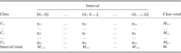
Each supervised discretization algorithm uses a criterion to evaluate a given discretization scheme. The most common way to store information about distribution of data points in the scheme is to use a [k + 1] x [n + 1] dimensional matrix (called the quanta matrix), which represents an exemplary discretization scheme with n intervals, k class labels, and M training instances, see Table 1. Each following column of the matrix stores information about the number of training instances in subsequent intervals. The rows represent the number of instances with subsequent class labels. In addition, the last row and last column hold aggregated information.
Two-dimensional quanta matrix for attribute F and discretization scheme D where qir is the number of training instances with i-th class label which are in r-th interval, Mi + is the number of all training instancess with i-th class label, and M +r corresponds to the number of all training instancess in r-th interval. two-dimensional quanta matrix for attribute F and discretization scheme D where qir is the number of training instances with i-th class label which are in r-th interval, Mi + is the number of all training instancess with i-th class label, and M +r corresponds to the number of all training instancess in r-th interval
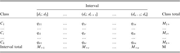
Given the quanta matrix Q for the attribute F and the discretization scheme D, we can define three probability values: pir, the probability of an instance from class i having a value in the rth interval of F; pi +, the probability of an instance belonging to ith class; and p +r, the probability of an instance having a value in the rth interval of attribute F. These probabilities are defined as:

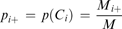
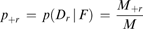
The following sections briefly describe discretization criterions which are used by the algorithms that are considered in this study.
2.2.1 Information entropy
Information entropy is a measure of uncertainty/indetermination associated with the random variable. In the case of discretization, it represents the amount of information which is needed to describe the scheme. The lower the entropy is, the better the scheme, as we need less information to describe it. Entropy is defined as

where if pir = 0 then  Entropy is non-negative and reaches a maximum when all probabilities have the same values.
2.2.2 Class-attribute interdependence redundancy and class-attribute interdependence uncertainty
CAIR (class-attribute interdependence redundancy; Wong & Liu, Reference Wong and Liu1975) and CAIU (class-attribute interdependence uncertainty; Huang, Reference Huang1996) criterions measure interdependence between class labels and generated intervals. Both criterions are insensitive to the number of class labels and distinct values. In the case of CAIR, bigger criterion value corresponds to stronger correlation between classes and intervals, while for CAIU this relation is reversed.
CAIR criterion is given by

where Ent(C,D |F) is the information entropy and I(C,D |F) is the class-attribute mutual information defined as

As for CAIU, the criterion is expressed by:

where Ent(C,D |F) is the information entropy and INFO(C,D|F) is the class-attribute information defined as

2.2.3 Class-attribute interdependency maximization
CAIM (class-attribute interdependency maximization) criterion was proposed in Kurgan and Cios (Reference Kurgan and Cios2004). This criterion generates intervals that contain as many instances assigned to only one of the class labels as possible. In other words, this criterion aims to generate intervals for which a dominant associated class can be found. Larger CAIM value corresponds to bigger correlation between classes and intervals. The CAIM criterion is defined as
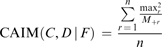
where maxr is the maximal value of qir (for i in the range [0; S]) in the r-th interval; in other words, maxr is the number of instances of the most frequent class label in the r-th interval.
The values of this criterion range between 0 and M. Value maxr 2 is divided by M +r to scale this value and to reward intervals with only one dominating class. The numerator is divided by the number of intervals n to generate discretization schemes with a small number of intervals.
2.2.4 Class-attribute contingency coefficient
Similar to the CAIM criterion, the CACC (Class-attribute contingency coefficient) criterion aims to generate schemes that maximize interdependence between class labels and intervals (Tsai et al., Reference Tsai, Lee and Yang2008). In contrast to CAIM, which favors schemes with a small number of intervals, CACC is more likely to accept schemes with a larger number of intervals, thus potentially further increasing interdependence.
This criterion is given by

where y is defined as
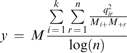
The variable y is divided by log(n) to reward schemes with a smaller number of intervals. We note that in Equation (9), division by n similarly aims at minimizing the number of intervals. The authors of the CACC criterion intentionally used log(n) instead of n to reduce the influence of this factor.
2.2.5 χ 2 criterion
The χ 2 criterion (Kerber, Reference Kerber1992) is based on the statistical χ 2test that is used to evaluate the hypothesis of class attribute independence. The χ 2 criterion value corresponds to the distance between the observed and expected frequencies of instances, and can be interpreted as the distance to the hypothesis of independence between attributes. The χ 2 criterion is defined as
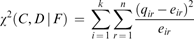
where expected frequencies eir are calculated as

If the hypothesis is true, then the χ 2-value is distributed like a χ 2 statistic with (n−1) × (k−1) degrees of freedom. A higher χ 2-value corresponds to lower confidence in the tested hypothesis.
2.2.6 MODL criterion
The MODL criterion, which has been introduced in (Boullé, Reference Boullé2006), combines the Bayesian approach and MDL (minimal description length) model (Rissanen, Reference Rissanen1978). The goal of the Bayesian approach is to maximize the probability P(Model | Data), which, with the use of Bayesian rules and considering that P(Data) is constant, is equivalent to maximizing

Provided that the calculation of the probabilities P(Model) and P(Data|Model) is feasible, the Bayesian approach finds an optimal model for the data.
By applying the MDL model, the Bayesian approach is reused replacing the probabilities with their negative logarithms, which can be interpreted as Shannon code lengths. This coding problem is solved by finding a model that minimizes:

The above problem can be calculated by finding the scheme that minimizes the following equation (Boullé, Reference Boullé2006):

Algorithms that use this criterion to search for the best schema should only compute the differences between criterion values after and before splitting an interval or merging two adjacent intervals. This is computationally more efficient than computing the criterion value from scratch.
2.3 Selected discretization algorithms
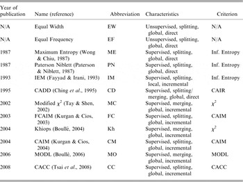
We selected a total of 12 discretization algorithms that cover various discretization approaches, see Table 2. We included several older algorithms such as two unsupervised methods, equal width and equal frequency, and four commonly used supervised methods, Maximum Entropy (ME) (Wong & Chiu, Reference Wong and Chiu1987), Information Entropy Maximization (IEM) (Fayyad & Irani, Reference Fayyad and Irani1993), Paterson Niblett (Paterson & Niblett, Reference Paterson and Niblett1987), and CADD (Ching et al., Reference Ching, Wong and Chan1995). The main reason for their inclusion is the fact that these methods are commonly used as a benchmark set for modern discretization algorithms (Kurgan & Cios, Reference Kurgan and Cios2001; Liu et al., Reference Liu, Hussain, Tan and Dash2002; Kurgan & Cios, Reference Kurgan and Cios2003, Reference Kurgan and Cios2004; Abraham et al., Reference Abraham, Simha and Iyengar2006; Boullé, Reference Boullé2006). Most of the older algorithms, except IEM, are direct, that is, they require the user to specify the final number of intervals. The newer algorithms are incremental. In the case of the direct methods, we use the following equation to determine the number of intervals:

where M is the number of distinct values of F and k is the number of class labels (Wong & Chiu, Reference Wong and Chiu1987; Kurgan & Cios, Reference Kurgan and Cios2004). When implementing the Paterson–Niblett algorithm, we used d and k to compute the maximum and minimum number of intervals, respectively.
Comparison of the 12 discretization algorithms used in the research

The simplest algorithms are unsupervised and they include the Equal Width and Equal Frequency algorithms. Both are direct methods which need a user to determine the number of intervals in the final scheme. The Equal Width method finds a minimal and a maximal value of F and divides the corresponding interval into d equally wide intervals. The Equal Frequency algorithm sorts the values of F and computes d intervals that contain the same number of values.
ME first uses the Equal Frequency algorithm to create d intervals and then perturbs interval borders as long as the perturbation increases the entropy. At each step, only the perturbation of one border that corresponds to the largest increase in the entropy is accepted.
CADD works similarly to ME, but instead of maximizing entropy, it tries to increase the value of the CAIR criterion. It also adds one more step in which some neighboring intervals are merged.
Paterson Niblett is a splitting algorithm which starts with one big interval and successfully divides it into smaller ones. In each cycle, a cut point that corresponds to the largest entropy gain is chosen. This method is driven by the user who must determine both the minimum and maximum number of intervals. After reaching the minimal number of intervals, the algorithm checks whether the next division will improve entropy; otherwise, it terminates. If the entropy value increases, then the algorithm terminates upon reaching the maximum number of intervals.
IEM is also a top-down algorithm but it uses only the data within a given interval to decide whether the interval should be divided. After every division of an interval, the method recursively checks whether the two new subintervals should be divided. It terminates when there are no more intervals to be divided.
We also included six modern discretization algorithms including Modified χ 2 (Tay & Shen, Reference Tay and Shen2002), CAIM (Kurgan & Cios, Reference Kurgan and Cios2004), FCAIM (Kurgan & Cios, Reference Kurgan and Cios2003), Khiops (Boullé, Reference Boullé2004), MODL (Boullé, Reference Boullé2006), and CACC (Tsai et al., Reference Tsai, Lee and Yang2008).
Modified χ 2 is an improvement of the χ 2 algorithm (Liu & Setiono, Reference Liu and Setiono1997). This is a bottom-up method which in each iteration decides, based on the χ 2 test, whether the two best adjacent intervals should be merged.
The class-attribute interdependence maximization (CAIM) and Fast CAIM (FCAIM) methods are both top-down methods that iteratively add boundary points by accepting a boundary, from among all midpoints, that maximizes the value of the CAIM criterion. The difference between these algorithms is that FCAIM uses a smaller set of potential boundary points that consists of midpoints between adjacent unique values that have different class labels, whereas the CAIM algorithm uses all midpoints.
The Khiops algorithm is a bottom-up method which uses the χ 2 statistic to choose a pair of intervals that maximize the χ 2-value when merged. To shorten the execution time, this method exploits the fact that the χ 2 criterion is additive. The criterion value for each interval is stored as it will not change until this interval is merged and only the values that concern the merged intervals are updated.
The MODL algorithm uses the MODL criterion which is based on the Bayesian approach, and thus it seems to be the best suited toward application with NB classifiers. It uses a technique similar to Khiops to speed up the computations. It also applies a greedy postoptimization based on the hill-climbing algorithm to find the most optimal discretization scheme.
Finally, we include one of the most recent discretization methods, CACC, which is a top-down method based on the CAIM algorithm that uses the CACC criterion when adding boundary points.
2.4 Naïve Bayes and semi-Naïve Bayes classifiers
Classification is the task in which a training set of t instances described by n features is used to build a model that is used to predict the class label y∈c 1,…,ck for a test instance x = 〈x 1,…,xn〉, where xi is the value of the i-th feature and k is the number of class labels.
2.4.1 Naïve Bayes and Flexible Naïve Bayes
The NB classifier assumes independency of features given a class label and performs classification using:
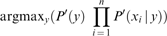
where P(y) and P(xi|y) are estimates of the respective probabilities derived from the training set. For nominal features, the conditional probabilities correspond to the probability of the i-th feature having the value of xi for a given class label, whereas for continuous features NB uses Gaussian distribution to model them and to estimate the probability. The maximum likelihood estimates of the mean and the standard deviation of the normal distributions are based on the sample average and standard deviation for each class label. Therefore, when the continuous features do not obey the Gaussian distribution, the estimates may lead to classification errors. To this end, a flexible NB, which improves the estimation of probability distribution for continuous features, was developed (John & Langley, Reference John and Langley1995). In this case, the distribution is averaged over a set of Gaussian kernels, where their number equals the number of values of the i-th feature in class ci and which have a mean equal to xi and the same standard deviation equal to  where tci corresponds to the number of instances in class ci. While NB and FNB accept continuous features, the remaining NB-derived classifiers considered require front-end discretization of continuous features.
2.4.2 Lazy Bayes rule
Lazy Bayes rule (LBR; Zheng & Webb, Reference Zheng and Webb2000) is an extension to NB in which the assumption of features independence is relaxed. Instead of using all features for a given class, LBR selects a subset of features W and the independence is assumed only among this subset and the class label. In this case, the classification is performed using:

W is selected using a heuristic wrapper that aims at minimizing error on the training data set (Zheng & Webb, Reference Zheng and Webb2000). The selection of the subset is delayed to the classification step and it relies on the data collected at the training step. This results in an increase in complexity, that is, the complexity of the classification step equals O(tkn 3).
2.4.3 Averaged one-dependence estimators
The estimation of W in LBR is time-consuming and thus a new algorithm, averaged one-dependence estimators (AODE), which relaxes the assumption of features independence that is used in the original NB, was developed (Webb et al., Reference Webb, Boughton and Wang2005). AODE is based on an ensemble of 1-dependence NB classifiers, that is, NB that assumes dependence on y and one feature xi

where F(xi) is a count of the number of training instances having the attribute value xi. To avoid false probability distributions, AODE averages only the models where F(xi) > 30, a minimum sample size that is widely used in statistics.
2.4.4 Hidden Naïve Bayes
The hidden Naïve Bayes (HNB) classifier also attempts to relax the assumption of the independence of the features (Zhang et al., Reference Zhang, Jiang and Su2005). For each attribute, this classifier creates a hidden parent which represents the influence of all other attributes. The hidden parent node is essentially a mixture of the weighted influences from all other attributes, where the weight is used to represent the importance of a given attribute. The weight can be either computed or manually assigned by a human expert.
2.4.5 Weightily averaged one-dependence estimators
Weightily averaged one-dependence estimators (WAODE) extends the AODE algorithm by varying the impact of each feature (Jiang & Zhang, Reference Jiang and Zhang2006). While AODE treats each tree-augmented NB equally, WAODE adds a weight for each 1-dependence NB classifier. The weight is computed using correlation between a given feature and the class variable.
2.4.6 Efficient lazy elimination for averaged one-dependence estimators
This classifier is designed upon an observation that correlated features can degrade NB’s accuracy. To this end, a new technique called lazy elimination (LE), whose goal is to identify and eliminate pairs of features where one feature is a generalization of the other feature, was developed (Zheng & Webb, Reference Zheng and Webb2006). During the training, the LE creates a table of probability estimates and the algorithm delays the elimination to the classification step. Based on attribute values of the instance that is being classified, LE deletes all features that are related to this instance. Since the information which is computed by LE during the training step is the same as the information collected by the AODE algorithm, the LE technique was coupled with AODE. At the same time, the LE technique can be used with any Bayesian classifier.
We note that besides the abovementioned classifiers, a few other NB-based classifiers were proposed. They include selective NB (SBC; Langley & Sage, Reference Langley and Sage1994), tree augmented Naive Bayes (TAN), and Super Parent TAN (SP-TAN) (Friedman et al., Reference Friedman, Geiger, Goldszmidt, Provan, Langley and Smyth1997). SBC uses forward feature selection to find a suitable subset of attributes that are used to construct the NB. The results presented in (Zhang et al., Reference Zhang, Jiang and Su2005) show that SBC is outperformed by HNB and hence the former method was not included in our study. SP-TAN is a variant of TAN in which the conditional independence between the features is relaxed and where each feature depends on the class label and one other (the so-called parent) feature. The parent feature is selected based on conditional mutual information (Keogh & Pazzani, Reference Keogh and Pazzani1999). The SP-TAN classifier was shown to provide accuracy comparable to LBR (Wang & Webb, Reference Wang and Webb2002) and thus it was also excluded from our study.
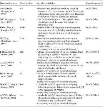
The NB and semi-NB classifiers are summarized in Table 3. The table also gives the computational complexity of the training (generation of the classification model on the training data set) and classification (time to apply the classification model on a test set) performed with these classifiers. We observe that all the considered methods have linear training time with respect to the number of training instances, although some of them scale in a non-linear fashion (either quadratic or cubic) with respect to the number of features. In addition, the LBR method performs poorly in the context of the classification time.
Comparison and main characteristics of the nine considered Naïve Bayes and semi-Naïve Bayes classifiers. k is the number of classes, t is the number of training instances, n is the number of attributes, and v is the average number of distinct values for an attribute; tr stands for training and cl stands for classification

3 Experimental results
All algorithms were implemented in JAVA. The classifiers used in the research were implemented in the WEKA workbench (Witten & Frank, Reference Witten and Frank2005), while we used in-house implementations for the discretization algorithms.
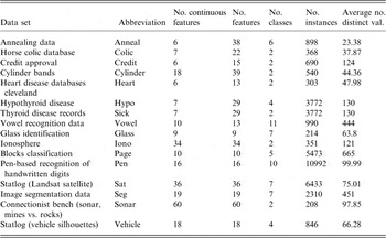
We used 16 data sets from a UCI repository (Asuncion & Newman, Reference Asuncion and Newman2007), see Table 4. We selected data sets that cover a wide range of problems including different numbers of classes (between 2 and 11), instances (between 208 and 10 992), and features (between 9 and 60). The top eight data sets include mixed feature types, that is, both continuous and nominal, while the bottom eight data sets include only continuous features.
Benchmark data sets used in the experiments

Since WAODE and HNB classifiers cannot handle missing values, we replace them with averages (for numerical features) and modes (for nominal features). The same procedure for imputation of missing values was implemented by the authors of these classifiers (Zhang et al., Reference Zhang, Jiang and Su2005; Jiang & Zhang, Reference Jiang and Zhang2006).
The experiments are based on five repetitions of twofold cross-validation, as suggested in Alpaydin (Reference Alpaydin1999), which results in a total of 10 folds (classifications). Each data set in each of the cross-validations was discretized by all 12 algorithms using only one (training) fold to create the discretization scheme. For each setup, that is, discretization algorithm and a data set, we computed the average CAIR (Ching et al., Reference Ching, Wong and Chan1995) and entropy values, as well as the average time needed to perform discretization and the average number of discretization intervals for each continuous feature. These values are used to evaluate and compare individual discretization algorithms.
Next, we use both the discretized and the raw data to evaluate the impact of discretization on the subsequently performed classification with NB and semi-NB classifiers. We use NB and FNB classifiers on the raw data and NB and the remaining considered semi-NB classifiers on the discretized data (we note that for the discrete data FNB is equivalent to NB). We train classifiers on the same fold that was used to derive the discretization scheme. For each setup, that is, classifier and a discretized/original data set, we compute average time to train the classification model (training time) on the training fold, and average accuracy and average time to use the model to classify the test samples (classification time) using the test fold. We note that training and test folds are of the same size.
The results are presented in two subsections. In the first subsection, we compare discretization methods based on the generated discretization schemes. In the second subsection, we compare and analyze the impact of discretization on the accuracies of the classifiers and the time needed to complete the entire process, that is, time to discretize the data, train a classification model, and classify the test fold.
3.1 Comparison of discretization algorithms
For each data set, the considered 12 discretization algorithms are compared based on the average CAIR and entropy values (over 10-folds using five repetitions of 2-fold cross-validation), which are used to quantify the quality of the generated discretization schemes, average running time (over 10-folds), and average number of intervals (over all continuous features and folds).
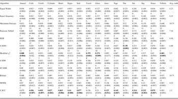
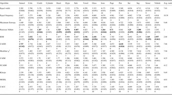
CAIR values quantify the interdependence between the discretized feature and the class labels such that higher values are associated with stronger relation between these two features. The discretization schemes with the highest CAIR values, see Table 5, are generated by CACC algorithm, followed by CAIM, FCAIM, and MODL. The worst results are obtained for Maximum Entropy, Khiops, and both unsupervised algorithms. The best entropy values, that is, higher entropy values indicate weaker relation between the discretized feature and the class labels, see Table 6, were obtained by the Paterson–Niblett and IEM algorithms. Again, the FCAIM, CAIM, and MODL algorithms scored relatively well. The worst results were obtained by the Equal Width, Maximum Entropy, and Khiops algorithms. We observe that although the results obtained with CAIR and Entropy differ, that is, these measures focus on different aspects of discretization, a few generic conclusions can be drawn. CAIM, FCAIM, and MODL perform well for both quality measures, while Khiops, Maximum Entropy, and both unsupervised methods score relatively poorly. This observation is supported by the fact that the unsupervised methods are very simple and thus they cannot perform as well as the supervised algorithms. Similar observations were made in Kurgan and Cios (Reference Kurgan and Cios2004), but they concerned a smaller set of seven discretization methods. The tables show that CAIM, FCAIM, and MODL rank consistently well across all data sets, while the performance of other methods such as modified χ 2 and CADD varies between the data sets. Some discretizers, including CACC, IEM, and Patterson–Niblett, score very well for one criterion, while the quality of their schemes is shown to be poor when evaluated with the other measure.
The average CAIR values associated with the discretization performed by the 12 discretization algorithms on the 16 benchmark data sets; higher CAIR value indicates better discretization scheme. The values in round brackets indicate standard deviation (over the 10-folds). The values in third row show rank of a given discretization algorithm for a given data set. Values in bold indicate the best results for a given data set. Last column shows average rank of a given algorithm over all data sets. Abbreviations for data set names can be found in Table 4

The average Entropy values associated with the discretization performed by the twelve discretization algorithms on the 16 benchmark datasets; lower entropy value corresponds to better discretization scheme. The values in round brackets indicate standard deviation (over the 10-folds). The values in third row show rank of a given discretization algorithm for a given data set. Values in bold indicate the best results for a given data set. Last column shows average rank of a given algorithm scored over all data sets. Abbreviations for data set names can be found in Table 4

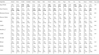
The results concerning the average time of the discretization process, see Table 7, show (as expected) that the two unsupervised methods are the fastest. Although theoretically the Equal Width algorithm is faster than the Equal Frequency since it does not require sorting of feature values, we had to sort the values to compute the number of intervals d. As a result, both of the unsupervised methods have virtually identical running time. We note that if the user would specify the number of the intervals, the Equal Width algorithm, which is the only method that has linear complexity with respect to the number of feature values, would be the fastest.
The average running time (ms) associated with the discretization performed by the 12 discretization algorithms on the 16 benchmark data sets. The values in round brackets indicate standard deviation (over the 10-folds). The values in third row show rank of a given discretization algorithm for a given data set. Bolded values indicate the best results for a given data set. Last column shows average rank of a given algorithm scored over all data sets. Abbreviations for data set names can be found in Table 4

The fastest supervised algorithm is FCAIM followed by CAIM and IEM. The slowest methods include MODL followed by Modified χ 2 and CADD. These numerical results stem from the design of these methods, that is, merging methods are in general slower than splitting methods. In addition, as shown in Table 8, the CAIM, FCAIM, and IEM methods generate a small number of intervals, which further improves their speed when compared with the other splitting methods. We observe that some differences are relatively large. For instance, for the page data set, which is characterized by the largest average number of distinct values, the unsupervised methods are two to three times faster than the fastest supervised methods, and they are three orders of magnitude faster than the slowest supervised methods. In the case of the pen data set, which has the largest number of instances, the fastest supervised and unsupervised discretizers are characterized by similar running time, while they are an order of magnitude faster than the slowest supervised methods.
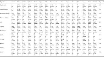
The average number of intervals for a continuous feature associated with the discretization performed by the 12 discretization algorithms on the 16 benchmark data sets. The values in round brackets indicate standard deviation (over the 10-folds). The values in third row show rank of a given discretization algorithm for a given data set. Values in bold indicate the smallest number of intervals for a given data set. Last column shows average rank of a given algorithm scored over all data sets. Abbreviations for data set names can be found in Table 4

In the next section, we aggregate the running time of the discretizers with the time required to build the classification model on the discretized data and the time to perform classification on the test fold to give further insights on the impact of discretization on the subsequent classification.
Table 8 gives the average number of intervals per continuous feature generated by the 12 algorithms. In general, schemes with a lower number of intervals cannot be considered better than schemes with a higher number because this information would have to be coupled with the information that quantifies how well these intervals describe the data distribution (e.g. CAIR or Entropy). However, if the distribution of the data is described equally well by two different discretization schemes, one should prefer the smaller scheme. We observe that the smallest schemes are generated by the IEM, FCAIM, CAIM, and MODL algorithms. For these algorithms, the number of intervals is often close to the number of classes in a given data set. We stress that the schemes generated by FCAIM, CAIM, and MODL are also characterized by favorable CAIR and entropy values. However, the biggest numbers of discretization intervals are generated by both unsupervised algorithms and by Maximum Entropy, Khiops, and Modified χ 2 algorithms. For unsupervised algorithms as well as for the Maximum Entropy, Paterson–Niblett, and CADD algorithms, the number of intervals is defined using the formula proposed in Wong and Chiu (Reference Wong and Chiu1987); however, the supervised algorithms merge some of these intervals reducing the resulting number of discretization intervals. The Khiops and ME discretizers also obtain poor CAIR and entropy values, see Tables 5 and 6, which indicate that these schemes are characterized by relatively poor quality. Our results show that Modified χ 2 generates schemes with a large number of intervals when dealing with large data sets such as vowel, seg, and pen, which is consistent with findings in (Tay & Shen, Reference Tay and Shen2002).
Overall, we conclude that the best trade-off between the running time, the quality of the discretization scheme expressed using CAIR and Entropy, and the number of discretization intervals is achieved by the FCAIM, CAIM, and IEM algorithms. The MODL method has a drawback of being relatively slow, but it also generates high quality discretization schemes. However, the worst performing methods include the two unsupervised methods, as well as Maximum Entropy, and Khiops, although these methods are relatively fast.
3.2 Classification with Naïve Bayes and semi-Naïve Bayes algorithms
We compare 6 classifiers on the data discretized by the 12 discretization algorithms, and two classifiers on the raw data. Hence, we have generated 74 different setups (classifier and discretizer pairs). Each setup was run on all 16 data sets where for each data set we performed five twofold cross-validations, that is, a total of ten test folds for each data set was considered for each set. Owing to their excessive size, the tables that provide all results are available online at http://biomine.ece.ualberta.ca/discretizationNB/. The results are summarized using the Friedman F-test and Nemenyi test, as suggested in (Demšar, Reference Demšar2006). These tests allow one to compare the quality of classifiers (measured using accuracy) across multiple data sets and to show the corresponding results in a convenient graphical format.
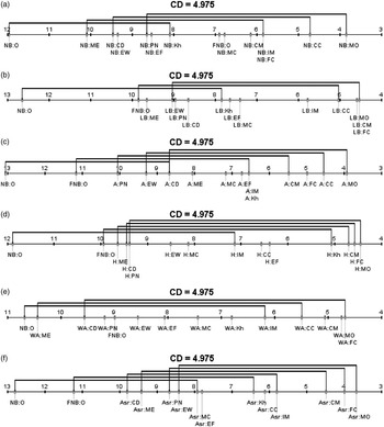
First, we compare accuracy using the Friedman F-test (Iman & Davenport, Reference Iman and Davenport1980). This test checks the null hypothesis whether accuracies of the considered classifiers are statistically equal based on the average place scored by a classifier along all data sets. If the null hypothesis is rejected, then a post hoc test (the Nemenyi test (Nemenyi, Reference Nemenyi1963)) is performed. This test orders the classifiers according to their quality and allows the selection of subsets of classifiers that are statistically undistinguishable, that is, classifiers for which the accuracies are not statistically significantly different. The best performing classifier is the method which has the lowest rank; this method is located in the rightmost position on a Nemenyi test figure. The worst classifier has the highest rank and is located in the left far end of a Nemenyi test figure. The setups for which ranks differ by less than the CD value are statistically indistinguishable from one another for the considered set of classifier accuracies obtained on a given set of data sets. The Nemenyi test figures use the abbreviated names of the discretizers and classifiers that can be found in Tables 2 and 3, respectively.
Two sets of tests are performed. First, we compare the impact of the 12 discretization methods on the accuracy of the same classifier. We also compare these results against baseline setups in which NB and FNB are run on the raw data. Second, we perform the test when considering all 74 setups together. For all performed tests, the null hypothesis was rejected, and hence we perform the post hoc test and present the corresponding graphical representation.
The results for NB classifier, see Figure 1(a), show that the accuracy of this classifier can be significantly improved by using discretization. This confirms the results obtained in previous studies (Flores et al., Reference Flores, Inza and Larran2007; Lee, Reference Lee2007). At the same time, for six discretization schemes, which were generated by the two unsupervised algorithms and the Maximum Entropy, CADD, Paterson–Niblett, and Khiops supervised algorithms, there is no statistical difference between the accuracies of the NB run on the raw data and on the discretized data. This means that in the context of the classification accuracy, usage of these discretizers would not benefit the user. However, a statistically significant difference is found for the remaining discretization algorithms including Modified χ 2, CAIM, IEM, FCAIM, CACC, and MODL and also when using the FNB classifier. The Nemenyi test also shows that the classification accuracies of classifiers generated with FNB, and classifiers generated using NB on the data discretized with Paterson–Niblett, Equal Frequency, Khiops, Modified χ 2, CAIM, IEM, FCAIM, CACC, and MODL are characterized by statistically insignificant differences. We observe that discretization with any of the considered 12 methods does not lead to statistically significant improvement when compared with results obtained with FNB. The five best performing discretizers for the NB classifier, that is, the methods that achieve the lowest ranks, are MODL, CACC, IEM, and FCAIM ex aequo, and CAIM.
Graphical representation of the Nemenyi test performed for results obtained by NB and FNB run on the 16 original data sets. The results for the Naïve Bayes, LBR, AODE, HNB, WAODE, and AODEsr classifiers are shown in panels (a, b, c, d, e), and (f), respectively, and they concern runs on the 16 data sets discretized by the 12 discretization algorithms. The best result is obtained by the setup with the lowest rank; CD is the critical value which determines whether different setups are statistically different. The sets of classifiers that are not significantly different are shown using the horizontal lines. The considered setups are shown in the x:y form where x denotes a classifier and y denotes a discretization method; abbreviations for x and y can be found in Tables 2 and 3, respectively. O denotes the original (raw) data

LBR is a classifier which works only with discrete data. This method is applied on the data discretized by the 12 discretizers and is compared against the NB and FNB classifiers that use the raw data. The results for the LBR classifier, see Figure 1(b), show that the results obtained on the discretized data are better than the results obtained by both the NB and FNB classifiers on the raw data. The results obtained for the data discretized by the five discretization algorithms (Maximum Entropy, Equal Width, Paterson–Niblett, CADD, and Khiops) are not statistically significantly better than the results obtained with NB. Statistically significant improvements over NB were obtained by using the remaining seven discretizers. The setups that are statistically significantly better than the results of both NB and FNB incorporate discretization with MODL, CAIM, and FCAIM. The five best results for the LBR classifier were obtained for schemes generated by the same discretization algorithms as the top five for the NB algorithm.
For the AODE classifier, see Figure 1(c), all the results obtained on the discretized data are again better than the results obtained by NB and FNB. We observe that three setups, which concern the Paterson–Niblett, Equal Width, and CADD discretizers, generate classification models with accuracies that are not statistically significantly higher that the accuracies of the NB classifier on the raw data. The four setups that are significantly better than both NB and FNB use data discretized with MODL, CACC, FCAIM, and CAIM. These four setups are also included in the top five list for the NB and LBR classifier. The IEM algorithm is also in the top five list for the AODE classifier, but this time it occupies this spot ex aequo with the Khiops algorithm.
In the case of the HNB classifier, see Figure 1(d), we yet again observe that the setups which incorporate discretization perform better than the classification models generated by the NB and FNB classifiers on the raw data. This time, however, six setups are not significantly better than NB. The setup with the IEM algorithm, which is in the top five lists for all other classifiers, placed seventh. The setups that are significantly better than both NB and FNB applied on the raw data use data discretized with MODL, FCAIM, and CAIM. For the HNB classifier, the top five setups differ from the setup that scores best for others classifiers. More specifically, the IEM and CACC algorithms are replaced by the Equal Frequency and Khiops algorithms. However, the top three setups are consistent and they are based on the MODL, FCAIM, and CAIM algorithms.
Figure 1(e) presents results for the WAODE classifier. Only four setups are shown to be significantly better than the results obtained with the NB classifier. These setups include discretization performed with the FCAIM, MODL, CAIM, and CACC algorithms. We also observe that the results obtained by this classifier using the discretized data are not significantly better than the results obtained with FNB. There are three setups which obtained worse scores than FNB, and they are based on the Maximum Entropy, CADD, and Paterson–Niblett algorithms. The five best setups for WAODE are consistent with the top scoring setups for the NB, LBR, AODE, and AODEsr classifiers.
Results for the AODEsr classifier that are given in Figure 1(f) again show that NB and FNB executed on the raw data achieve the worst accuracies. Nevertheless, five setups are not significantly better than NB (CADD, Maximum Entropy, Paterson Niblett, Equal Width, and Modified χ 2) and the top five setups are statistically better than both NB and FNB. The latter group includes MODL, FCAIM, CAIM, IEM, and CACC, which is consistent with the top five lists of all other classifiers except HNB.
Overall, the results show that NB executed on the raw data is outperformed by NB and semi-NB classifiers that use discretized data. For all classifiers, except WODE and NB, the second worst rank was obtained by the FNB classifier, that is, discretization performed within FNB is outperformed by discretization performed by the considered 12 methods. The top five setups for all classifiers, except HNB, include the same five discretization algorithms, MODL, FCAIM, CAIM, IEM, and CACC. Moreover, the setups that incorporate these algorithms are always significantly better than the results obtained by using NB on the raw data; the only exception is the setup that includes IEM and WAODE. In the case of the HNB classifier, the best three setups include the MODL, FCAIM, and CAIM algorithms, and these discretizers are in the top three setups when considering other classifiers; except for NB where they are in the top five and AODE where CAIM is fourth. The results achieved by all setups that incorporate the unsupervised methods and older supervised methods, except IEM, were almost always comparable (not significantly better) with the results obtained by applying NB and FNB on the raw data. This shows that recently developed discretizers provide a significant improvement when compared with the older method. The setups with the two discretization methods based on χ 2 criterion (Modified χ 2 and Khiops) scored in the middle of the considered setups. At the same time, usage of the Khiops algorithm gave better results than setups that are based on the Modified χ 2 algorithm for all but the NB and LBR classifiers.
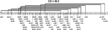
Figure 2 summarizes the results of the Nemenyi test for all considered setups. The large CD values are due to the large number of setups, that is, 74, when compared with the number of data sets, that is, 16. In spite of that, we observe that the results which are significantly better than the worst results that are obtained using NB on the raw data include almost all setups with the three discretization algorithms, MODL, FCAIM, and CAIM; only the setups with the NB classifiers are not in this group. However, all setups that use the NB classifier on the discretized data are shown to be comparable with the results obtained with the NB on the raw data. The setups which include the AODEsr and AODE classifiers (except the setup with the Paterson–Niblett discretizer) are among the best results. The best three setups which are on the far right end of the plot are setups that couple the AODEsr classifier with the MODL, FCAIM, and CAIM discretization algorithms. The big gap between these three and the remaining setups demonstrates a relatively big improvement between the scores of this group and the fourth and subsequent setups.
Graphical representation of the Nemenyi test performed for results obtained by NB and FNB run on the 16 original data sets, and the results for the 6 classifiers run on the 16 data sets discretized by the 12 discretization algorithms. The best result is obtained by the setup with the lowest rank; CD is the critical value which determines whether different setups are statistically different. The sets of classifiers that are not significantly different are shown using horizontal lines. The considered setups are shown in the x:y form where x denotes a classifier and y denotes a discretization method; abbreviations for x and y can be found in Tables 3 and 2, respectively. O denotes the original (raw) data

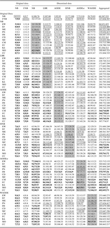
An alternative way to compare the accuracies is to count the wins, draws, and losses which a given setup achieves when compared against all other setups on all data sets (Demšar, Reference Demšar2006), that is, we compared each setup against every other setup on each data set. To compare whether a given setup is better than another setup, we used the combined 5 × 2 cv F-test (Alpaydin, Reference Alpaydin1999), that is, a win and a loss indicate that the difference is statistically significant. The table that gives all results can be found at http://biomine.ece.ualberta.ca/discretizationNB/. It compares all setups against the scores achieved by every classifier, that is, for each classifier, it sums up all wins, draws, and losses that a given setup achieves against all setups built using a given classifier. Table 9 summarizes the results by comparing a given setup with the aggregated (across all setups) results of another classifier. If the classifier is also used in the considered setup, then we can analyze how well a given discretization algorithm compares against all other discretization algorithms used with this classifier. We also compute a coefficient WDLC
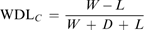
where W, D, L stand for the number of wins, draws, and losses, respectively, and c indicates a given setup. If the coefficient value is bigger than 0, then the corresponding setup wins more often than it loses, whereas when the value is smaller than 0, the setup suffers more losses than wins. A value of 0 indicates an equal number of wins and losses. The coefficient values range between −1, that is, a given setup always loses, and 1, that is, a given setup always wins. The coefficients across all setups sum up to 0 since the number of wins and losses is equal. To better visualize the differences in Table 8, the cells, where WDLC is bigger than 0.2, are given in bold. However, the cells that correspond to setups with WDLC that is lower than −0.2 are underlined.
Number of wins, draws, and losses, respectively, achieved by a setup in a given row when compared against all setups (using all discretization methods) for a given classifier shown in the column. The setups include NB or FNB classifier run on the 16 raw data sets and each of the six classifiers run on the 16 data sets discretized by each of the 12 discretization algorithms. Bolded scores show WDLC scores greater than 0.2; underlined scores correspond to WDLC scores smaller than −0.2. Gray shading indicates comparison between setups that use the same classifier. The last column contains the aggregated, over all other setups, scores for a given setup. Abbreviations for algorithms and classifiers names can be found in Tables 2 and 3, respectively

The setup that includes the NB classifier on the raw data is shown to often lose with other setups (it loses 553 times and wins only 68 times). Similarly, all setups with the NB classifier and discretized data register more losses than wins. The two best classifiers are AODE and AODEsr. The setups that involve these classifiers are almost always characterized by more wins than losses.
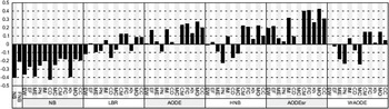
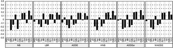
The WDLC values are visualized in Figures 3 and 4. The former figure gives the coefficient values when comparing a given setup against all other setups that use a different classifier, while the latter figure shows the values when comparing a given setup against all other setups that use the same classifier. As such, Figure 3 allows comparison between a given setup and other classifiers and Figure 4 enables comparison of different discretization algorithms for the same classifier.
WDLC values for all considered setups. The values are based on comparison with all other setups except the setups that include the same classifier. The setups include NB or FNB executed on the 16 raw data sets and each of the 6 classifiers on the 16 data sets discretized by each of the 12 algorithms. Abbreviations for algorithms and classifier names can be found in Tables 2 and 3, respectively

WDLC values for all considered setups. The values are based on comparison among setups that are based on the same classifier. The setups include NB or FNB executed on the 16 raw data sets and each of the six classifiers on the 16 data sets discretized by each of the 12 algorithms. Abbreviations for algorithms and classifier names can be found in Tables 2 and 3, respectively

Figure 3 shows that the best results along all considered classifiers were obtained by the AODEsr classifier for which all setups have a positive coefficient (the coefficient for the setup which includes a Modified χ 2 discretizer is positive and close to 0). On the opposite end, all coefficient values for the NB classifier are negative. Relatively good scores were also obtained with the AODE and HNB classifiers.
Most importantly, we observe that the scores obtained by each classifier strongly depend on the discretization method used to discretize the input data. Figure 4 shows that five discretizers, which include MODL, FCAIM, CAIM, IEM, and CACC, generate the highest and always positive values across all considered classifiers. However, several algorithms such as Maximum Entropy, Paterson–Niblett, CADD, and Modified χ 2 always obtain negative coefficient values. The latter group incorporates relatively old algorithms, except for the Modified χ 2. The remaining algorithms have a similar number of losses and wins. The above conclusions are similar to the observation derived when using the Freidman F and Nemenyi tests.
3.3 Running time analysis
We also investigate the trade-off between the classification accuracy and the running time necessary to compute the discretization scheme and the classification model, and to compute predictions for the test instances. We note that the classification model is built only once, while it can be used to classify an unlimited number of test instances. This motivates us to consider the time to predict the test instances. In addition, we note that some of the semi-NB classifiers, such as LBR, are characterized by higher complexity associated with the prediction, see Table 3.
Similarly, as in the case of the classification model, the discretization process is performed only once before a classifier is built. After that, the generated discretization scheme can be used to discretize multiple samples. The time needed to discretize a single instance with a given scheme is directly proportional to the number of continuous attributes and the number of intervals in a given scheme. Therefore, the smaller the average number of intervals in a given scheme is, the faster the discretization process is. We observe that this time is negligible when compared to the time necessary to compute the scheme and the classifier, that is, the conversion into the discrete feature uses a pre-computed look up table that represents the discretization scheme, and thus we disregard it in our analysis.
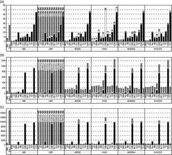
Owing to the limited amount of space, our analysis is based on three data sets. We choose the smallest (glass), the average size (hypo), and the biggest (pen) data sets. The remaining plots are given on http://biomine.ece.ualberta.ca/discretizationNB/. The plots show the average time (over the five twofold cross-validation experiments) to build the discretization scheme using black bars, the average time to train a classifier using white bars, and the average time to classify a test set using gray bars. We focus on the analysis of the training and prediction times since the discretization time was already discussed in the context of Table 7.
Figure 5(a) summarizes the results for the smallest data set. It shows that the process to compute the discretization scheme can be time-consuming when compared with the time needed to build the classification model and to classify the test instances. However, the time needed to classify discretized instances by any classifier, except LBR, is generally lower than the time needed to classify the original instances, which is associated with the NB and FNB classifiers. Most importantly, we observe that the whole process of discretizing, training, and classifying data is almost always shorter, except for the setups that apply the CACC discretizer and the LBR classifier, than the process of training and classifying the raw data using the FNB classifier. This is particularly important in the context of the fact that the building of the discretization scheme and the classification model is done only once, whereas the time needed to classify test instances is additive.
Time plots for the glass, hypo and pen data sets are shown in panels (a, b), and (c), respectively. The y axis gives the time in milliseconds; the x axis lists all setups including NB and FNB executed on the raw data and the six classifiers run on the data discretized by each of the 12 algorithms. Black bars show the time of the discretization process on the training fold; white color represents the time to train the classification model on the training fold; gray color denotes the time needed to classify the test fold. Training and test folds have the same number of instances. Abbreviations for algorithms and classifier names can be found in Tables 2 and 3, respectively

The longest training time is required for the HNB classifier and it is also associated with the setups in which data were discretized with the Modified χ 2 algorithm. The latter is likely caused by the relatively large number of intervals generated for this particular data set by the Modified χ 2 method, see Table 8. The setups which incorporate the CACC and CADD discretizers need more time to build the classification model. Although the schemes generated by CACC include a relatively large number of intervals, this is not the case for the CADD algorithm. Therefore, we hypothesize that the reason for the long training time is poor quality of the corresponding schemes.
Figure 5(b) gives the results for the hypothyroid data sets. This data set has average size and it consists of seven continuous and 22 nominal features. Owing to the relatively small number of continuous features, the results show that the time to classify the raw instances by NB is shorter than the time necessary to generate classification with most of the discretization-based setups. Only the setups that use the NB classifier on the discretized data are faster than NB on the raw data. We again observe that the time to classify raw data by FNB is longer than the time needed to classify instances by most of the other classifiers, except LBR, that use the discretized data. The difference is not as large as for the glass data set since FNB is very efficient for nominal features that are present in the raw data set. The longest training time, that is, time to compute the classification model, is observed for HNB.
The results for the biggest data set are presented in Figure 5(c). This data set consists exclusively of continuous features. The observations are similar to the observations on the glass data set. The time to classify discretized data is generally lower than the time needed to classify the raw data by NB and FNB (except for the LBR classifier). This is especially transparent in the case of FNB that requires a substantial amount of time to predict the test instances. Most of the discretization times, except for the Paterson–Niblett, Modified χ 2, MODL, and CACC algorithms, are 5 to 10 times smaller than the time to classify the test set. The large number of intervals generated by the Modified χ 2 algorithm results in long training and classification times.
Similar conclusions can be drawn for the remaining data sets; see http://biomine.ece.ualberta.ca/discretizationNB/ for the time plots. The longest time to classify the test instances is observed for the LBR classifier. This time is almost always two orders of magnitude greater than the combined time to perform discretization and generation of the classifier. Discretization reduces the time to build the classifier and to predict the test instances. This is especially transparent for data sets that consist only of numerical (continuous) features, while for a few smaller mixed (both continuous and nominal features) data sets the benefits are not always as significant. We observe that the ratio between the discretization and classification times is smaller for bigger data sets. Classification with FNB most often takes more time than combined discretization and classification with semi-NB classifiers. For larger data sets that consist of continuous features, the usage of the discretization-classification combo, except when slow discretization methods such as MODL, Modified χ 2, and Paterson–Niblett are used, is also faster than the NB classifiers executed on the raw data.
4 Summary and conclusions
The comparison of the 12 considered discretizers indicates that unsupervised methods are faster than supervised methods. The fastest supervised algorithm is FCAIM followed by CAIM and IEM. The slowest is MODL followed by Modified χ 2 and CADD. The best overall quality measured over multiple dimensions, which include running time, quality of the discretization scheme expressed using CAIR and Entropy criteria, and the number of discretization intervals, is achieved by the FCAIM, CAIM, and IEM algorithms. Three algorithms, MODL, FCAIM, and CAIM, generate the smallest discretization schemes and achieve favorable CAIR and entropy values. The MODL method has a drawback of being relatively slow, but it also generates high-quality discretization schemes. The IEM algorithm is fast and generates small schemes with good Entropy and acceptable CAIR values. The worst performing methods include the two unsupervised methods, Equal Width and Equal Frequency, and the ME and Khiops algorithms. We also note that the Modified χ 2 algorithm generates a large number of discretization intervals.
Analysis of the impact of discretization on the classification with NB and semi-NB classifiers shows that discretization generally improves the accuracy when compared against NB and FNB run on the raw data. At the same time, we observe that the choice of the discretization algorithm impacts the significance of the improvement. The MODL, FCAIM, and CAIM methods have the biggest positive influence on the accuracy of the subsequent classification. Their application in tandem with most of the semi-NB classifiers results in statistically significant improvements. The IEM and CACC algorithms also guarantee a good improvement, which is slightly better than the improvement obtained with the Khiops algorithm. The unsupervised methods, as well as the Modified χ 2, Paterson–Niblett, CADD, and ME algorithms, produce relatively large discretization schemes, and provide the smallest improvements for the subsequent classification.
When analyzing the performance of the considered classifiers, we found that the most accurate models are generated by the AODEsr method followed by AODE and HNB. The classification accuracies obtained when combining AODEsr with the top performing discretizers that include MODL, FCAIM, and CAIM give statistically significant improvement over the classification performed with both classical NB methods, NB and FNB. The worst accuracies are obtained when using the original NB followed by FNB and LBR.
We found that the results of the evaluation of the discretization methods correlate with the accuracy of the classification performed on the discretized data, that is, well scoring discretizers provide good quality data, which in turn results in improved accuracies (irrespective of the type of classifier used). This shows that the quality indices used to evaluate discretization schemes can be used to indicate the quality of the classification with the NB-based classifiers.
Investigation into the impact of discretization on the classification time shows that although the time needed to build the discretization scheme could be longer than the time needed to train the classifier, the time to classify the discretized instances (that includes the time to discretize data, compute the classifier, and predict the test instances) is often shorter than the time needed to classify continuous instances. We show that the time needed to classify test instances is an important factor that is strongly influenced by discretization. At the same time, the time needed to build the classification model is not as strongly influenced by discretization.
We show that discretization not only has a positive impact on the accuracy of NB and semi-NB models, but it also has a positive impact on their classification time, that is, a strong positive influence is observed in the context of the time needed to classify an instance. The magnitude of this influence varies depending on which method was used to derive the discretization scheme. We found that the biggest positive influence, both on the accuracy and the classification time, is associated with three algorithms that generate the smallest discretization schemes, MODL, FCAIM, and CAIM.
Acknowledgements
This work was supported in part by the NSERC Discovery grant to L. Kurgan and by the Killam Memorial Scholarship to M. J. Mizianty.