1. Introduction
Vortex-induced vibration (VIV) is a canonical flow–structure interaction phenomenon in long, flexible structures with bluff cross-sections, capable of causing severe fatigue damage and compromising long-term structural integrity (Blackburn & Henderson Reference Blackburn and Henderson1999; Grouthier et al. Reference Grouthier, Michelin, Modarres-Sadeghi and de Langre2013). Accurate prediction of the VIV response is therefore essential for ensuring structural reliability and developing effective maintenance strategies.
Vortex-induced vibration has been extensively investigated, spanning canonical flows past rigid cylinders to the more complex responses of flexible cylinders in uniform currents, as comprehensively reviewed in recent literature (Williamson & Govardhan Reference Xia, Ren, Guo, Liu, Lin and Wang2004; Liu et al. Reference Lucor, Imas and Karniadakis2020; Wang et al. Reference Williamson and Govardhan2020; Huera-Huarte Reference Huera-Huarte2025). Classical investigations established fundamental mechanisms, including mode competition and overlap, multi-frequency response and lock-in, wherein the wake velocity oscillation frequency coincides with the structural vibration frequency (Lehn Reference Leweke and Provansal2003; Vandiver et al. Reference Wang, Fan and Lin2005; Chaplin et al. Reference Chaplin, Bearman, Huarte and Pattenden2005; Huera-Huarte & Bearman Reference Huera-Huarte and Bearman2009a
; Seyed-Aghazadeh & Modarres-Sadeghi Reference Shang, Stone and Smits2016; Zheng & Wang Reference Zhu, Hu, Gao, Zhao and Xu2022; Lin et al. Reference Lin and Wang2024). Building on these foundations, subsequent research has increasingly focused on VIV in non-uniform flows. For oscillating rigid cylinders in shear currents, Stansby (Reference Techet, Hover and Triantafyllow1976) identified spanwise lock-in cells whose characteristic length increases with vibration amplitude, a trend later observed in oscillating cables (Peltzer & Rooney Reference Ren, Wang, Lin and Fan1985). Such localised lock-in arises where the vortex-shedding frequency matches the local structural frequency, whereas frequency mismatch corresponds to non-lock-in states. Direct numerical simulations further revealed that flexible cylinders in linear shear exhibit standing-wave responses dominated by a single frequency (Lucor et al. Reference Lucor, Mukundan and Triantafyllou2001, Reference Ma and Srinil2006), while exponential shear induces mixed standing–travelling waves and broadband spectra, with lock-in preferentially occurring in high-velocity regions. Extending this, Bourguet et al. (Reference Bourguet, Karniadakis and Triantafyllou2011a
,
Reference Bourguet, Modarres-Sadeghi, Karniadakis and Triantafylloub
) demonstrated that tensioned cylinders with large aspect ratios Reynolds number (
 $Re=110$
–
 $1100$
) support travelling waves propagating from high- to low-velocity regions, with lock-in confined to high-velocity zones where counter-clockwise figure-eight orbits emerge. Furthermore, Bourguet, Karniadakis & Triantafyllou (Reference Bourguet, Karniadakis and Triantafyllou2013) showed that broadband responses in exponential shear correspond to distributed lock-in events along the span: for narrowband excitation, lock-in remains localised to high-velocity regions, whereas for broadband cases, it may extend across the entire span, including low-velocity zones. Collectively, these studies demonstrate that non-uniform inflows introduce pronounced spanwise variations in the VIV response of flexible cylinders.
However, the VIV of flexible structures with curvature or catenary geometries, which frequently arise in deep-sea applications such as underwater target detection and deep-water oil production, has received comparatively little attention. The presence of curvature introduces non-uniform tension and spanwise variations in local flow velocity, giving rise to a strong flow–curvature coupling that fundamentally alters the fluid–structure interaction relative to straight and tensioned cylinders (Srinil et al. Reference Stansby2009, Reference Srinil, Wiercigroch and O’Brien2018). Direct numerical simulations of concave curved cylinders have revealed spanwise-dependent wake regimes, including oblique shedding, vortex dislocations and multiple shedding frequencies (Gallardo, Andersson & Pettersen Reference Gallardo, Andersson and Pettersen2014; Jiang et al. Reference Kim, Vandiver and Holler2018), consistent with experimental observations (Shang, Stone & Smits Reference Spalart and Leonard2018). Direct numerical simulations of turbulent flow around curved tandem cylinders further identified multistable regimes with coexisting Strouhal numbers, underscoring the strong influence of curvature on the vortex dynamics and instability interactions (Aasland et al. Reference Aasland, Pettersen, Andersson and Jiang2022a
,
Reference Aasland, Pettersen, Andersson and Jiangb
, Reference Aasland, Pettersen, Andersson and Jiang2024). Investigations of curved cylinders free to oscillate in one (Seyed-Aghazadeh, Budz & Modarres-Sadeghi Reference Seyed-Aghazadeh and Modarres-Sadeghi2015) or two degrees of freedom (Assi et al. Reference Assi, Srinil, Freire and Korkischko2014) revealed that both concave and convex geometries produced smaller vibration amplitudes than vertical cylinders. More recently, Seyed-Aghazadeh et al. (Reference Seyed-Aghazadeh, Budz and Modarres-Sadeghi2021) observed that vortex shedding along curved flexible cylinders with low mass ratios evolves both temporally and spatially along the span for concave and convex orientations alike. Catenary-type risers (CTRs), a canonical example of slender catenary configurations, serve as critical conduits for oil and gas transportation between seabed pipelines and floating production systems. Their large aspect ratio and inherent geometric nonlinearity heighten susceptibility to VIV, yielding a complex spanwise response dynamics (Leweke & Provansal Reference Li, Chen, Gu and Bai1995; Srinil, Ma & Zhang Reference Srinil, Wiercigroch and O’Brien2018). Experimental studies by Morooka & Tsukada (Reference Pang, Zong, Zou and Wang2013) revealed spatio-temporal variations of cross-flow responses along the CTR span at moderate Reynolds numbers (
 $Re=400$
–
 $600$
), while Chaplin & King (Reference Chaplin and King2018) reported broader spectral responses with multiple distinct peaks compared with tensioned vertical risers. Extensive experiments by Zhu and co-workers further demonstrated that CTRs in shear flows exhibit spatially distributed multi-frequency responses, with dominant frequencies varying both along the span and over time due to spatial mode competition and temporal mode switching (Zhu et al. Reference Zhu, Lin and Yao2016, Reference Zhu, Lin and Yao2019a
,Reference Zhu, Zhang, Zhao, Xie, Tang and Zhou
b
, Reference Zhu, Lin and Gao2021).
While these studies have yielded valuable experimental insights, a mechanistic understanding of the spanwise-varying response and its dependence on geometric configuration and flow conditions remains incomplete. Moreover, the high computational cost and meshing complexity associated with computational fluid dynamics (CFD) limit its feasibility for systematic parametric exploration, thereby motivating the development of reduced-order modelling approaches for CTR VIV prediction. The proposal of the independence principle (IP), which assumes that structural vibrations are primarily governed by the normal component of the incoming flow and thus decouple the fluid and structural scales (Friehe & Schwarz Reference Friehe and Schwarz1968; Gabbai & Benaroya Reference Gabbai and Benaroya2005), has an effective framework to address this challenge. Bourguet, Karniadakis & Triantafyllou (Reference Bourguet, Karniadakis and Triantafyllou2015) demonstrated the validity of applying the IP locally along the span for flexible cylinders inclined at
 $60^{\circ }$
, even when local inclination angles reach
 $75^{\circ }$
due to in-line deformation. Miliou et al. (Reference Modarres-Sadeghi, Mukundan, Dahl, Hover and Triantafyllou2007) showed that sufficiently long vertical extensions promote wake alignment perpendicular to the free-stream direction, an effect that can be further enhanced by high axial tension and significant structural vibration (Mathelin & de Langre Reference Meng and Chen2005; Bourguet & Triantafyllou Reference Bourguet and Triantafyllou2016; Srinil et al. Reference Srinil, Wiercigroch and O’Brien2018). These findings broaden the range of applicability of the IP. Moreover, experiments by Zhu, Lin & Gao (Reference Zhu, Lin and Yao2019a
) further indicated that the VIV problem of a CTR in uniform flow can be approximated as that of a vertical cylinder subjected to the normal component of the free-stream velocity, since the IP is applicable over most of the span except near the lower region where the inflow velocity is very small. These studies collectively demonstrate the applicability of the IP combined with strip theory for VIV analysis of CTRs. Based on this framework, several reduced-order models have been developed to investigate CTR VIV under various conditions, including wake oscillator models (Srinil, Wiercigroch & O’Brien Reference Stansby2009; Ma & Srinil Reference Mathelin and de Langre2023; Liu et al. Reference Liu, Li, Qiu, Leng, Li and Li2024), the vector form intrinsic finite element model (Li et al. Reference Lie, Larsen and Tveit2021) and semi-empirical models (Lie, Larsen & Tveit Reference Lin, Sun, Liu, Zhu, Wang, Triantafyllou and Fan2001; Moe et al. Reference Morooka and Tsukada2004; Guo et al. Reference Guo, Yuan, Tang and Xue2021), all of which have shown good predictive capability. Parametric investigations based on these reduced-order frameworks have shown that curvature (Leclercq & de Langre Reference Lehn2018), inclination angle (Li et al. Reference Lie, Larsen and Tveit2021; Ma & Srinil Reference Mathelin and de Langre2023; Liu et al. Reference Liu, Li, Qiu, Leng, Li and Li2024), internal fluid velocity and top tension (Meng & Chen Reference Miliou, Vecchi, Sherwin and Graham2012) all exert significant influence on the maximum response amplitudes, mode transitions, frequency-locking regions, energy transfer and internal force distribution of CTRs. More recently, Xia et al. (Reference Zheng and Wang2025) developed a strip-theory-based discrete vortex method for curved flexible cylinders, which enables efficient prediction of unsteady hydrodynamic forces and wake structures without CFD meshing or empirical coefficients. Their simulations revealed a distinct modal-group switching behaviour in the VIV response of CTRs, arising from the competition among the multiple frequencies. Nevertheless, most existing numerical studies have focused primarily on global dynamic characteristics, while the mechanisms governing spanwise variations in the response remain largely unexplored. This gap highlights the need for a systematic investigation that directly connects the spanwise response characteristics with the geometric and flow parameters controlling the CTR dynamics.
Given these insights, several key questions remain: How are the mono-frequency and multi-frequency responses related? How do the incoming flow velocity and initial geometric configuration modulate the spanwise distribution of VIV characteristics? And what physical mechanisms govern these spanwise variations in the responses of CTRs? To address these questions, we numerically investigate the VIV of CTRs with different initial geometric configurations subjected to various uniform incoming velocities, using a strip-theory-based discrete vortex method. The present analysis elucidates the connection between mono- and multi-frequency responses and reveals the underlying mechanisms responsible for the spanwise distributed VIV behaviour, enabling a classification of the CTR span into three distinct response regions. These findings provide valuable implications for the design and fatigue management of CTR systems by identifying regions that warrant particular engineering attention.
The remainder of the paper is organised as follows. The methodology is outlined in
 $ \S$
2. The influence of the incoming flow velocity on the VIV response of CTRs is examined in § 3, while the effects of the initial geometric configuration are analysed in § 4, with particular emphasis on the underlying mechanisms of the distinct spanwise regimes (§ 4.3). Finally, the main conclusions are presented in § 5.
2. Methodology
2.1. Governing equations of the discrete vortex method
In the present strip-theory-based discrete vortex method (DVM), the incompressible viscous flow is governed by the vorticity transport equation, expressed as (2.1)
 \begin{equation} \frac {\partial \omega }{\partial t} + (\boldsymbol{V}\boldsymbol{\cdot }\boldsymbol{\nabla })\omega =\nu \bigtriangledown ^{2} \omega, \end{equation}
where
 $\boldsymbol{V}$
is the velocity vector,
 $\omega$
is the vorticity component which is the vorticity of
 $\boldsymbol{V}$
and
 $\upsilon$
is the fluid kinematic viscosity. Based on the operator-splitting method, (2.1) is decomposed into a convective term and a viscous diffusion term (Chorin Reference Chorin1973) as follows:
 \begin{align} \frac {\partial \omega }{\partial t} +(\boldsymbol{V}\boldsymbol{\cdot }\bigtriangledown )\omega =0,\end{align}
 \begin{align} \frac {\partial \omega }{\partial t} =\nu \bigtriangledown ^{2} \omega.\end{align}
Based on the vorticity–streamfunction formulation and the Biot–Savart law, the convection velocities of vortex elements are obtained as
 \begin{equation} \boldsymbol{V}(\boldsymbol{r}, t)=\boldsymbol{U}_{\infty }-\frac {1}{2 \pi } \sum _{i=1}^N \varGamma _i \frac {\left (\boldsymbol{r}-\boldsymbol{r}_i\right )}{\left (\boldsymbol{r}-\boldsymbol{r}_i\right )^2+\sigma _i^2}, \end{equation}
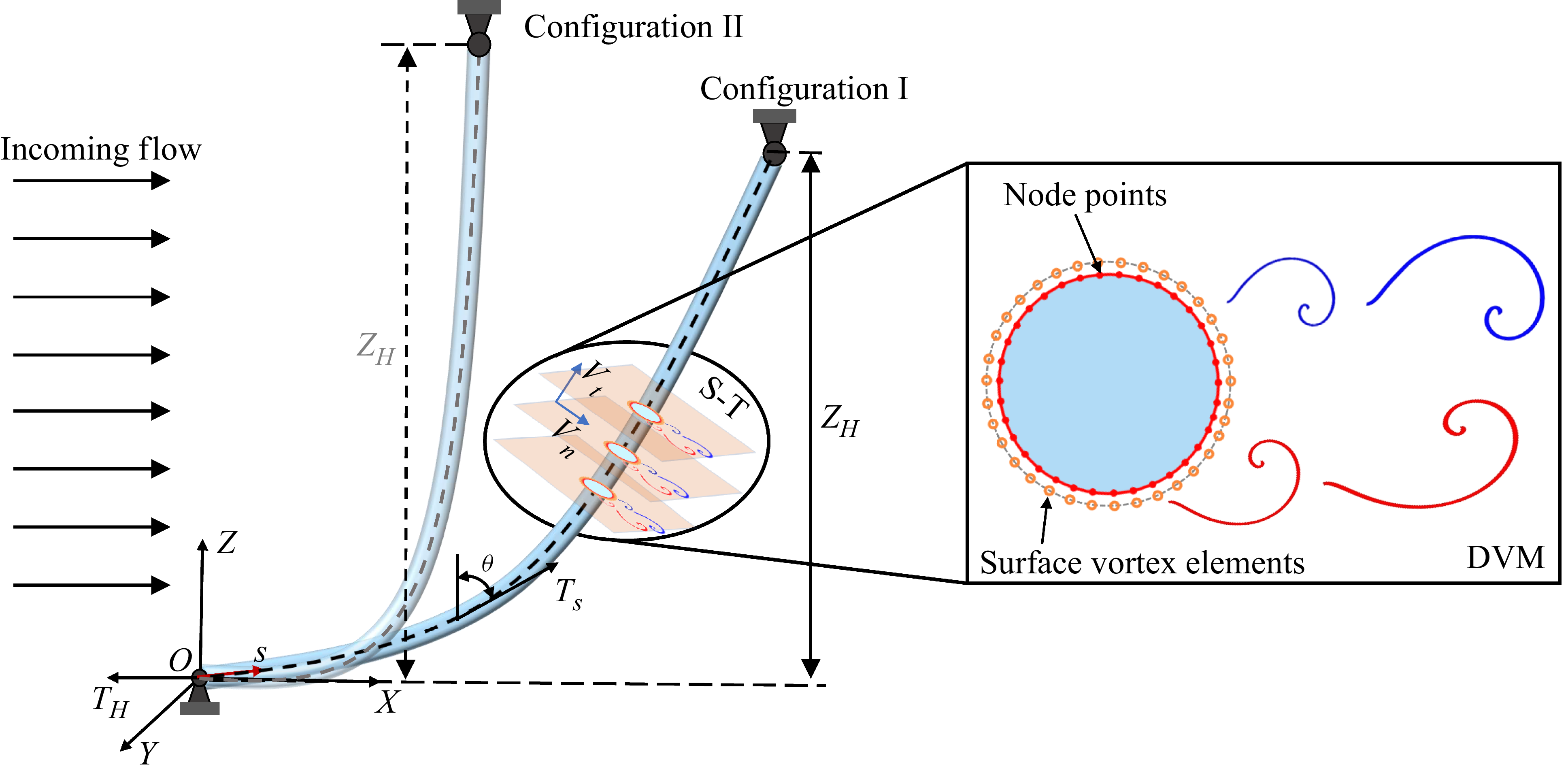
Schematic of the CTR geometry, illustrating two initial configurations (I and II) and the sketch of the strip-theory-based DVM.

where
 $N$
is the total number of vortex elements,
 $U_{\infty }$
is the incoming flow velocity,
 $\sigma _i$
represents the radius of the
 $i$
th vortex element, which was introduced by Chorin (Reference Chorin1973) to remove the singularity in vortex element formulations, and
 $\varGamma _i$
and
 $\boldsymbol{r}_i=(x_i,y_i)$
are the circulation and position of the
 $i$
th vortex element, respectively. To solve (2.3), the vortex core growth method (Park & Hifuchi Reference Peltzer and Rooney1989) is adopted, leading to the following expression:
 \begin{equation} \sigma ^{n+1} =\sqrt {(\sigma ^{n})^{2}+4.946\upsilon \Delta t}, \end{equation}
where
 $\Delta t$
denotes the time increment, while superscripts
 $n$
and
 $n+1$
correspond to the
 $n$
th and
 $(n+1)$
th time steps, respectively. The validity of this approach has been demonstrated in our earlier study (Lin & Wang Reference Lin, Wang, Fan and Triantafyllou2019; Xia et al. Reference Zheng and Wang2025).
The core concept of DVM is to approximate the continuous vorticity field by a series of discrete vortex elements with circulation. For the flow around a bluff body, vorticity originates from the development of the boundary layer. To mimic this process, surface vortex elements are generated on the body surface at corresponding node points to represent the vorticity produced within the boundary layer, as shown in figure 1. Once the release locations of these newly generated vortices are specified, their circulation is determined by solving a linear equations as
 $[\boldsymbol{A}]\boldsymbol{\varGamma }=[\boldsymbol{B}]$
, derived from the no-slip boundary condition (Xia et al. Reference Zheng and Wang2025). The elements of matrices
 $A$
and
 $B$
are defined as
 \begin{align} & \qquad\qquad\qquad a_{k i}=\frac {1}{4 \pi } \ln \frac {\left [\left (\boldsymbol{r}_{k+1}-\boldsymbol{r}_i\right )^2+\sigma _{i}^2\right ]}{\left [\left (\boldsymbol{r}_k-\boldsymbol{r}_i\right )^2+\sigma _{i}^2\right ]},\end{align}
 \begin{align} b_k & = \left (\boldsymbol{U}_{\infty }-\boldsymbol{U}_{k}\right )\left (\boldsymbol{r}_{k+1}-\boldsymbol{r}_k\right )-\frac {1}{4 \pi } \sum _{i=1}^{N_w} \varGamma _i \ln \frac {\left [\left (\boldsymbol{r}_{k+1}-\boldsymbol{r}_i\right )^2+\sigma _{i}^2\right ]}{\left [\left (\boldsymbol{r}_k-\boldsymbol{r}_i\right )^2+\sigma _{i}^2\right ]},\end{align}
where
 $\boldsymbol{U_k}$
is the body velocity at
 $k$
th surface node point,
 $N_w$
is the total number of vortex elements already present in the wake.
With the circulation obtained, the induced velocity of each vortex element is obtained from (2.4), and its trajectory is subsequently updated in a Lagrangian framework with (2.2) and (2.3). As the simulation progresses, vortex elements with identical circulation will aggregate to form the vortices in the wake. At each time step, new surface vortex elements are shed from the body surface, causing the total number of vortex elements to increase rapidly. This growth not only leads to excessive computational costs but also introduces redundant computations due to overlapping vortex elements. To address these issues, the vortex-merging criterion proposed by Spalart & Leonard (Reference Srinil, Ma and Zhang1981) is applied to reduce the number of vortex element while preserving the essential flow characteristics. Furthermore, to ensure the no-penetration condition at the body surface, the image vortex with correction boundary condition method developed by Pang et al. (Reference Park and Hifuchi2016) is adopted to properly handle the vortex elements that inadvertently penetrate into the body interior. The fluid pressure on the body surface is evaluated by performing a closed-loop line integral of the tangential pressure gradient, which is derived from the no-slip boundary condition, along the surface. From this procedure, the pressure relationship between
 $k$
th and
 $(k+1)$
th node points can be expressed as follows:
 \begin{equation} p_{k+1}=p_k+\rho \left ( -\frac {\varGamma _k}{\Delta t}-a_{tk}\Delta s\right )\!, \end{equation}
where
 $\Delta s$
denotes the length of the segment connecting the
 $k$
th and
 $(k+1)$
th node points and
 $a_{tk}$
is the tangential acceleration at the boundary of the
 $k$
th segment. The time-varying hydrodynamic forces on the structure are obtained by integrating the pressure distribution along the body surface, thereby overcoming the limitations of reduced-order models that depend on empirical hydrodynamic coefficients. The detailed solution procedure of the DVM is presented in our previous studies (Lin & Wang Reference Lin, Wang, Fan and Triantafyllou2019; Lin et al. Reference Liu, Ai, Sun and Soares2021; Ren et al. Reference Seyed-Aghazadeh, Benner and Gjokollari2024; Xia et al. Reference Zheng and Wang2025).
2.2. Governing equations of the structural responses
For flexible cylinders with very large aspect ratios, shear deformation is negligible compared with the bending deformation. Accordingly, in this work the structural dynamics is modelled using a tensioned Euler–Bernoulli beam with both ends fixed, as is commonly adopted in related studies (Bourguet et al. Reference Bourguet, Karniadakis and Triantafyllou2011a , Reference Bourguet, Modarres-Sadeghi, Karniadakis and Triantafylloub ; Lin & Wang Reference Lin, Wang, Fan and Triantafyllou2019; Zheng & Wang Reference Zhu, Hu, Gao, Zhao and Xu2022; Xia et al. Reference Zheng and Wang2025). The governing dynamic equation for the cylinder transverse response under hydrodynamic excitation can be expressed as
 \begin{align} m\frac {\partial ^2q_i(z,t)}{\partial t^2}+c\frac {\partial q_i(z,t)}{\partial t}+\frac {\partial ^2}{\partial z^2}\left (\! EI(z)\frac {\partial ^2q_i(z,t)}{\partial z^2}\right )-\frac {\partial }{\partial z}\left ( T(z,t)\frac {\partial q_i(z,t)}{\partial z}\right )\!=\!{f_q}_i(z,t), \end{align}
where
 $m$
denotes the mass of the cylinder per unit of length;
 $c$
is the damping of the cylinder;
 $E$
is the Young’s modulus and
 $I(z)$
is the moment of inertia of the structure;
 $q_i(z,t)$
represents the structural displacement in the in-line (IL) direction (
 $i=1$
) and the cross-flow (CF) direction (
 $i=2$
);
 ${f_q}_i(z,t)$
and
 $T(z,t)$
denote the hydrodynamic forces and the top tension, respectively. By discretising (2.9) with the finite element method, the structural governing equation is written as
 \begin{equation} \boldsymbol{[M]}\ddot {\boldsymbol{q}}+\boldsymbol{[B]}\dot {\boldsymbol{q}}+\boldsymbol{[K]}\boldsymbol{q}=\boldsymbol{[F(t)]}, \end{equation}
where
 $\boldsymbol{q}$
is the vector of displacement of the node, with
 $\dot {\boldsymbol{q}}$
and
 $\ddot {\boldsymbol{q}}$
representing the velocity and acceleration vectors, corresponding to the first- and second-order time derivatives of
 $\boldsymbol{q}$
, respectively. Here,
 $\boldsymbol{M}$
is the mass matrix,
 $\boldsymbol{B}$
is the damping matrix derived using the Rayleigh assumption and
 $\boldsymbol{K}$
is the stiffness matrix, consisting of both the elastic stiffness matrix
 $\boldsymbol{K_E}$
and the geometric stiffness matrix
 $\boldsymbol{K_G}$
, i.e.
 $\boldsymbol{K} = \boldsymbol{K_E} + \boldsymbol{K_G}$
. Also,
 $\mathbf{F}(t)$
represents the time-varying external loads induced by hydrodynamic forces on the structural elements. The structural dynamic equation is solved using the Hilbert–Huang Transform-
 $\alpha$
method scheme (Hughes Reference Jiang, Pettersen, Andersson, Kim and Kim1983), in which the parameters are defined as
 $0 \leqslant \alpha \leqslant 1/3$
,
 $\beta = (1 + \alpha )^2 / 4$
and
 $\gamma = 1/2 + \alpha$
.
2.3. Fluid–structure interaction framework and CTR parameters
Under self-weight loading, the CTR adopts a curved equilibrium configuration, where fluid–structure interactions mediated by curvature give rise to enhanced VIV complexity compared with straight risers (Srinil et al. Reference Srinil, Wiercigroch and O’Brien2018). Therefore, determining this initial configuration is a prerequisite for subsequent VIV analysis. Assuming a horizontal hinged bottom end, the initial configuration and axial tension can be obtained as (Xia et al. Reference Zheng and Wang2025)
 \begin{align} \theta & =arctan\left(\frac {T_H}{sW_e}\right),\end{align}
 \begin{align} T_s & = \sqrt {T_H^2+s^2W_e^2},\end{align}
 \begin{align} x=\frac {T_H}{We}arsinh\left(\frac {sW_e}{T_H}\right),&\quad z=\sqrt {\left(\frac {T_H}{W_e}\right)^2+s^2}-\frac {T_H}{W_e},\end{align}
where
 $\theta$
denotes the angle between the axial direction and the vertical plane;
 $T_s$
is the axial tension at a given position;
 $x$
and
 $z$
are the coordinates of a point on the CTRs in the Cartesian coordinate system (
 $X$
–
 $Y$
–
 $Z$
);
 $T_H$
is the constant horizontal static tension;
 $s$
is the length of the CTRs at a certain position; and
 $W_e$
is the effective weight of the CTRs fully immersed in water, defined as
 $W_e = (M_s - \rho \pi D^2 / 4)g$
.
As illustrated in figure 1, two initial configurations of the CTRs are presented. In this study, the initial configuration is not modified by altering the self-weight but by artificially varying the vertical subsea height
 $Z_H$
while keeping the total length unchanged. For example, increasing
 $Z_H$
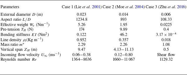
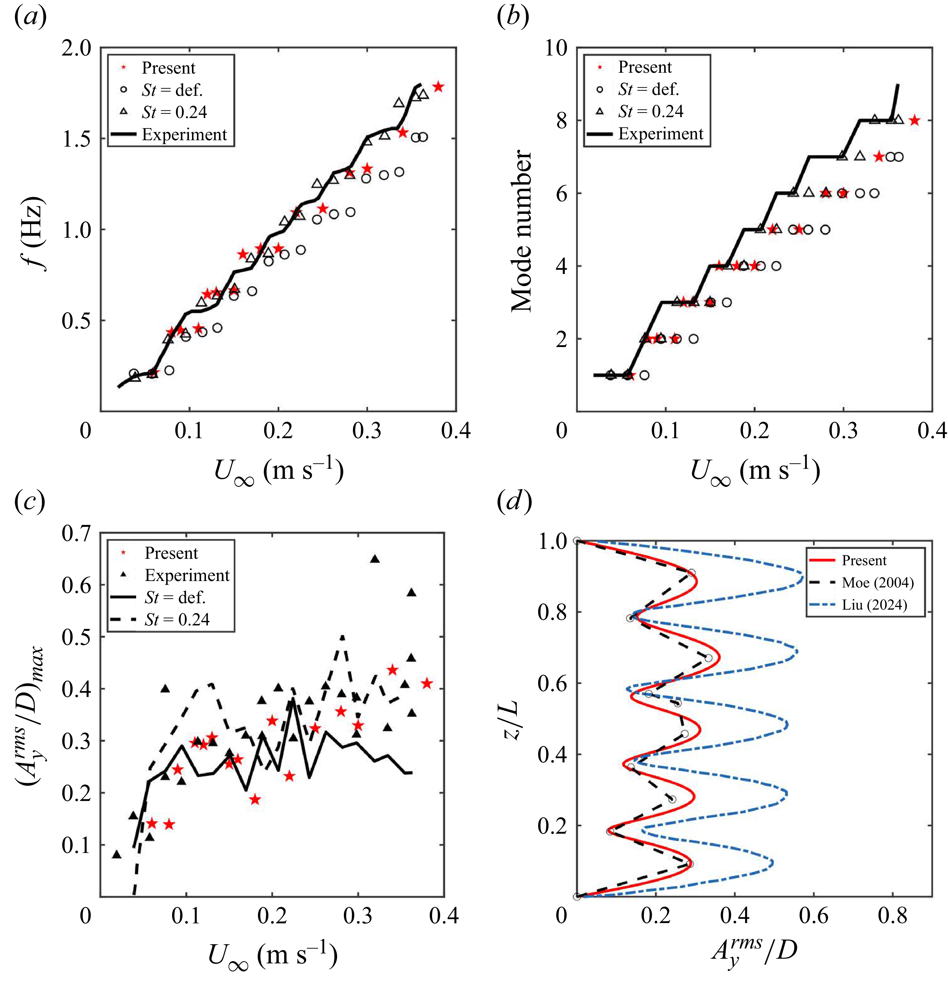
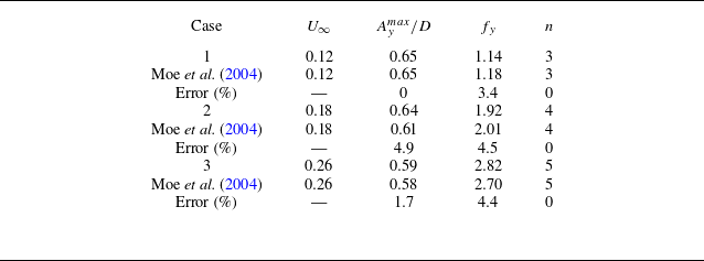
results in a transition from configuration I to configuration II. This approach provides a convenient means to obtain the desired configuration and facilitates a systematic analysis of how the initial geometry influences the VIV responses at different axial positions. The CTR parameters adopted in this work are consistent with those reported by Moe et al. (Reference Morooka and Tsukada2004), as summarised in table 1.
The main parameters of the CTRs adopted in the present work and Lie et al. (Reference Lin, Sun, Liu, Zhu, Wang, Triantafyllou and Fan2001), Moe et al. (Reference Morooka and Tsukada2004), Zhu et al. (Reference Zhu, Lin and Yao2016).

In the present fluid–structure interaction (FSI) framework, the strip-theory-based DVM is employed as a quasi-three-dimensional CFD model. Instead of solving the full-scale three-dimensional flow field, the flow is decomposed into a series of two-dimensional flow strips associated with the structural elements. Previous studies have shown that long structural extension (Miliou et al. Reference Modarres-Sadeghi, Mukundan, Dahl, Hover and Triantafyllou2007), high axial tension (Bourguet et al. Reference Bourguet, Karniadakis and Triantafyllou2015) and structural vibrations (Leclercq & de Langre Reference Lehn2018; Srinil et al. Reference Srinil, Wiercigroch and O’Brien2018) can all reduce three-dimensional flow effects of curved structures, thereby supporting the validity of this simplification. On each strip, the motion of vortex elements around the circular cross-section is computed using the DVM algorithm, thereby providing the hydrodynamic forces acting on the corresponding structural element, as described in § 2.1. Due to the curved geometry of the CTRs, the flow on each strip exhibits an inclination angle relative to the local axial direction, which significantly increases the numerical complexity. To address this issue, Zhu et al. (Reference Zhu, Lin and Yao2019a
) demonstrated experimentally the applicability of the IP for CTR configurations. Accordingly, the IP is adopted here by decomposing the incoming velocity into a normal component,
 $V_n = U_\infty \cos \theta$
, which dominates the FSI, and a tangential component
 $V_t = U_\infty \sin \theta$
, which is neglected (see circular inset in figure 1) (Friehe & Schwarz Reference Friehe and Schwarz1968). Then, the resulting hydrodynamic forces are then transferred to the structural solver to compute the global structural response, as outlined in § 2.2. Following the structural update, the new positions of the vortex elements on the surface are advanced according to the new configuration, and this process is iterated until the end of the simulation.
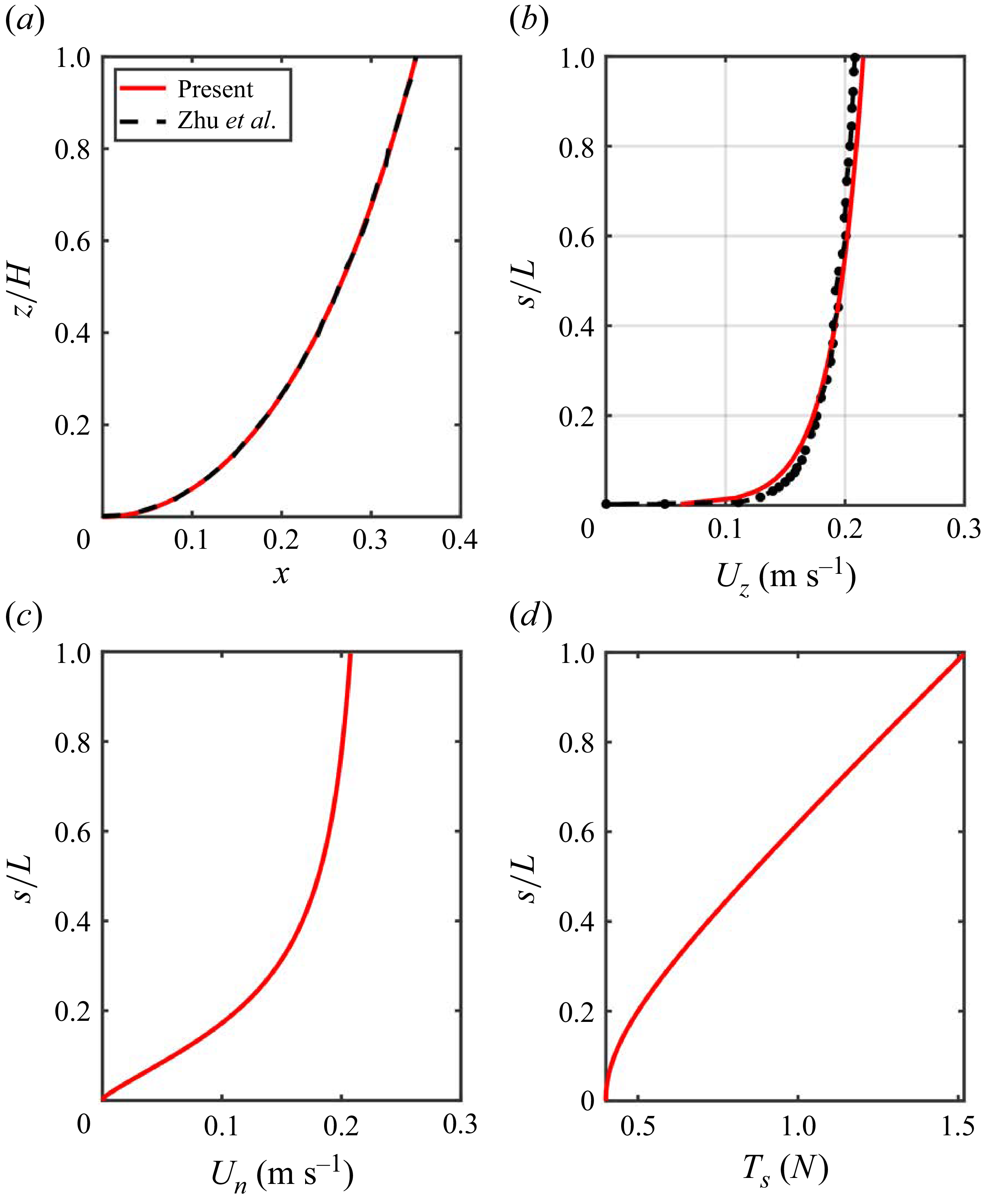
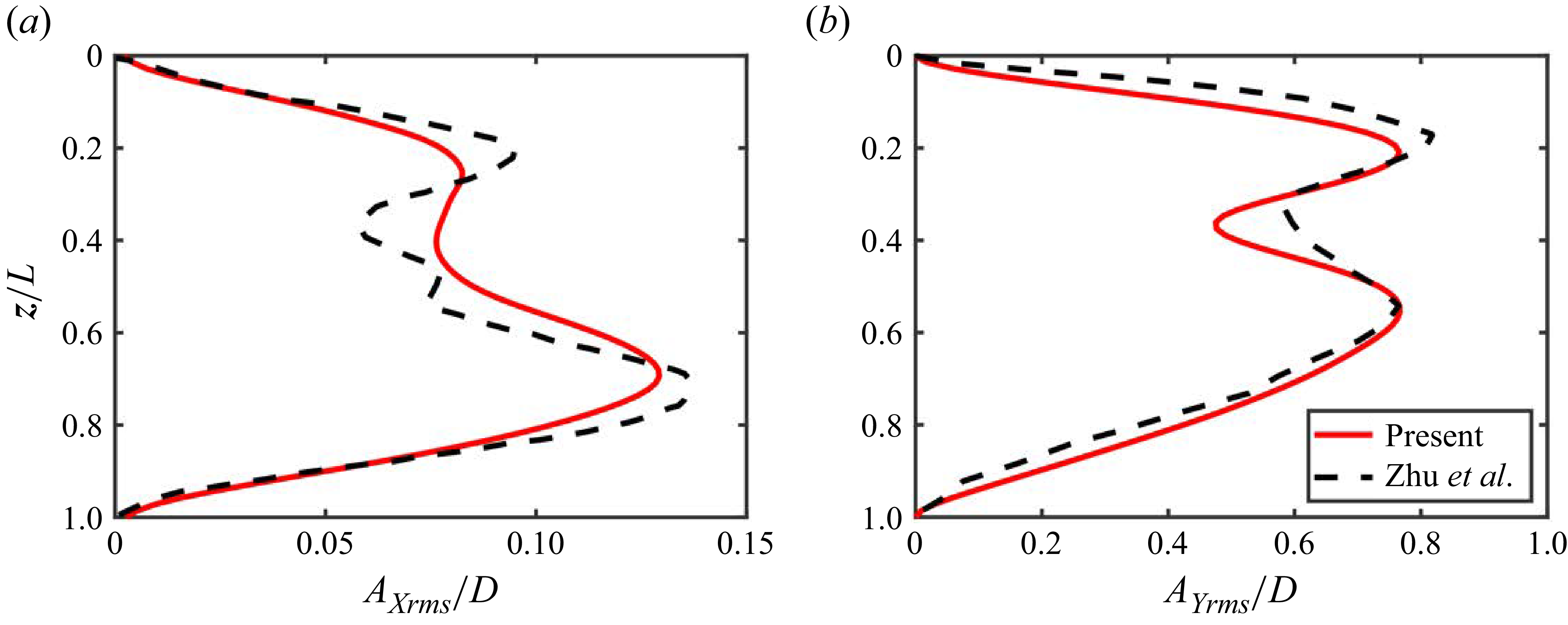
This modelling framework eliminates reliance on empirical hydrodynamic coefficients by directly resolving the instantaneous hydrodynamic forces acting on the structure, while at the same time offering substantial computational savings relative to full-scale three-dimensional simulations. The validation of the algorithm is presented in detail in the Appendix.
3. Vortex-induced vibration response of the CTRs under different incoming velocities
In this section, the spanwise variation of CTR VIV responses under different incoming flow velocities is examined. The frequency and CF displacement response is presented in § 3.1, with particular emphasis on clarifying the relationship between mono-frequency and multi-frequency responses during the modal-group transitions. Subsequently, § 3.2 analyses the characteristics of the FSI, focusing on the spanwise response features, within which three distinct spanwise regimes are identified. The modulation effect of the incoming velocity on the spanwise distribution of these regimes is then discussed in § 3.3. Finally, the vortex-shedding patterns corresponding to these regimes are illustrated in § 3.4.
3.1. Structural response characteristics
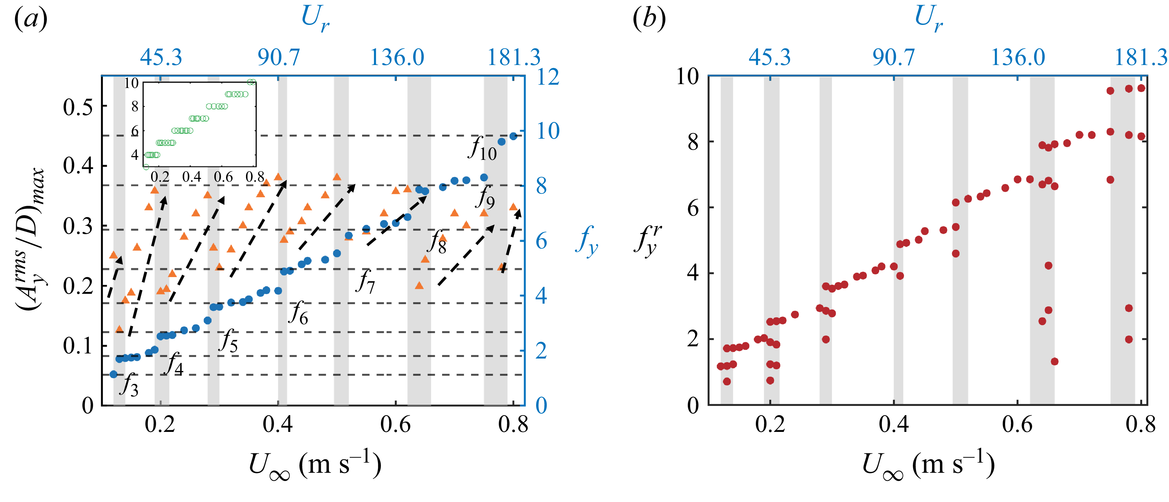
Investigating the characteristics of structural responses is a critical first step toward understanding the mechanisms of FSI. We first examined the maximum of the root-mean-square (r.m.s.) CF displacement,
 $(A_y^{rms}/D)_{max}$
, and the dominant response frequency,
 $f_y$
, over a range of incoming velocities fixed
 $Z_H=7.13$
, and the modal-group phenomenon is identified as shown in figure 2
 $(a)$
. Within each modal group, the dominant frequency remains locks onto the natural frequency of the corresponding mode number (dashed lines in figure 2
 $(a)$
), while
 $(A_y^{rms}/D)_{max}$
increases monotonically with the incoming velocity
 $U_{\infty }$
. During transitions between modal groups (grey shaded areas in figure 2
 $(a)$
), the dominant frequency shifts to the next higher mode as the mode number increases, accompanied by an abrupt drop in
 $(A_y^{rms}/D)_{max}$
. Meanwhile, the structural response contains multiple frequency components, in contrast to the mono-frequency response observed within the modal group, as illustrated in figure 2
 $(b)$
. Similar behaviour has also been reported for vertical flexible cylinders by Chaplin et al. (Reference Chaplin, Bearman, Huarte and Pattenden2005) in non-uniform currents and by Fan et al. (Reference Fan, Wang, Triantafyllou and Karniadakis2019) in uniform currents, where the phenomenon was interpreted in terms of the spatially averaged added-mass coefficient. In addition, Zhu et al. (Reference Zhu, Lin and Gao2021) and Xia et al. (Reference Zheng and Wang2025) observed comparable behaviour in experimental and numerical studies of catenary flexible risers, respectively. An important question is whether the structural responses differ between conditions within the modal group and in modal-transition region, as such comparisons are essential for elucidating the mechanisms underlying frequency switching and modal competition. To address this, we select three representative cases for detailed analysis:
 $U_{\infty }=0.38$
ms−1, located within sixth modal group, and
 $U_{\infty }=0.20$
and
 $0.65$
ms−1, corresponding to transitions from the fourth to fifth and from the eighth to ninth modal groups, respectively.
 $(a)$
Dominant frequency
 $f_y$
and maximum r.m.s. in CF displacement
 $(A_y^{rms}/D)_{max}$
of CTRs as functions of incoming velocity
 $U_{\infty }$
at
 $Z_H=7.13$
. The inset shows the corresponding mode number
 $n$
versus
 $U_{\infty }$
.
 $(b)$
Frequencies involved in the structure response
 $f_y^r$
as a function of
 $U_{\infty }$
, with the grey shading indicating the multi-frequency response region.

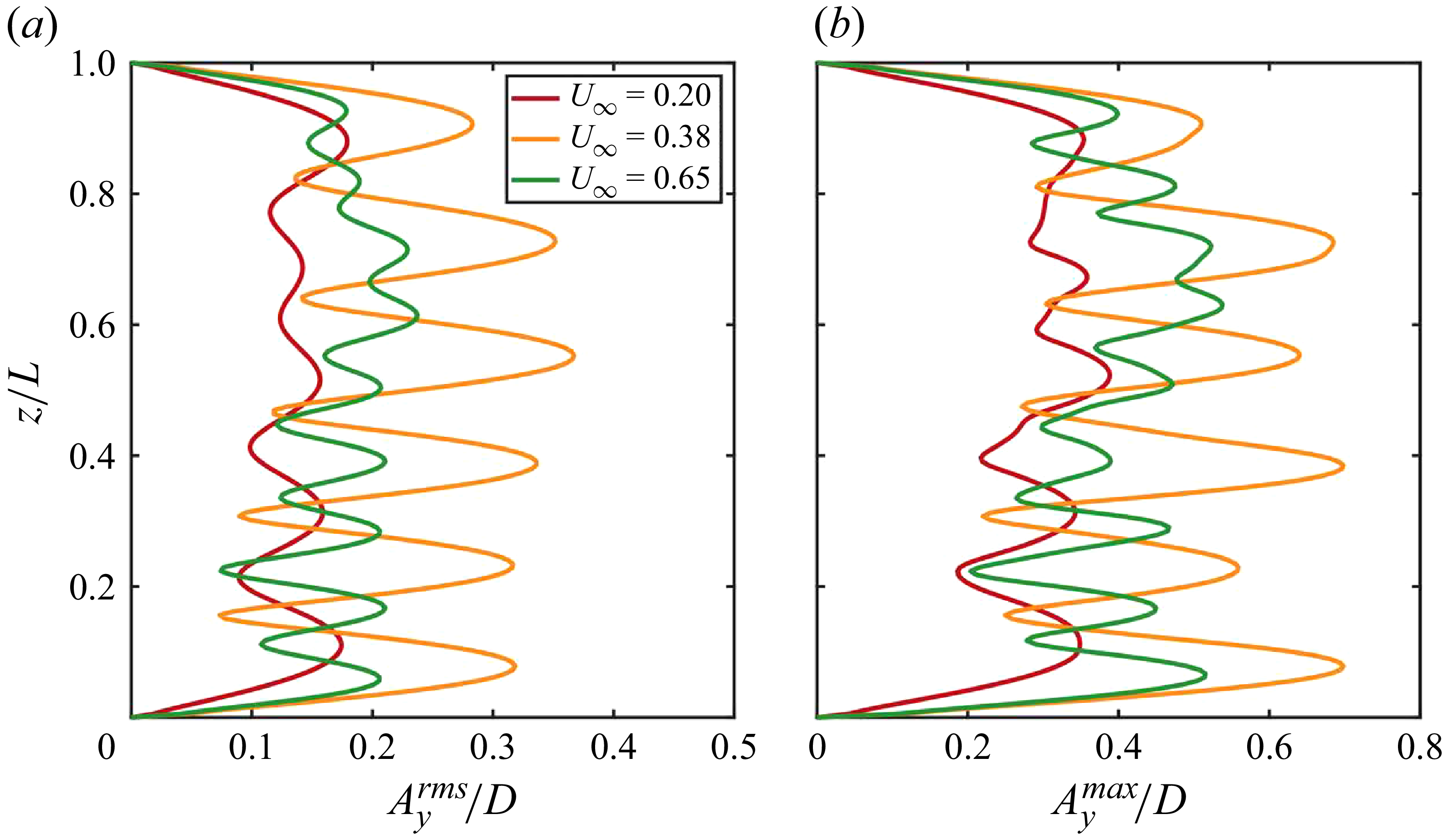
 $(a)$
The r.m.s. and
 $(b)$
maximum values of CF displacement along the CTR span at
 $U_{\infty }=0.20$
,
 $U_{\infty }=0.38$
and
 $U_{\infty }=0.65$
ms−1.

The
 $A_y^{rms}/D$
and
 $A_y^{max}/D$
values of the CF displacement along the CTR span at these representative incoming velocities are shown in figure 3. Both
 $A_y^{rms}/D$
and
 $A_y^{max}/D$
exhibit a mixed standing–travelling-wave pattern. The alternating distribution of ‘nodes’ (local minima) and ‘anti-nodes’ (local maxima) indicates the presence of standing waves, while the non-zero r.m.s. values at the nodes highlight the contribution of travelling waves. These results demonstrate that the mixed standing–travelling-wave patterns is an inherent feature of CTR VIV responses, consistent with previous findings in flexible cylinders (Lucor et al. Reference Lucor, Mukundan and Triantafyllou2001, Reference Ma and Srinil2006; Bourguet et al. Reference Bourguet, Karniadakis and Triantafyllou2011a
).
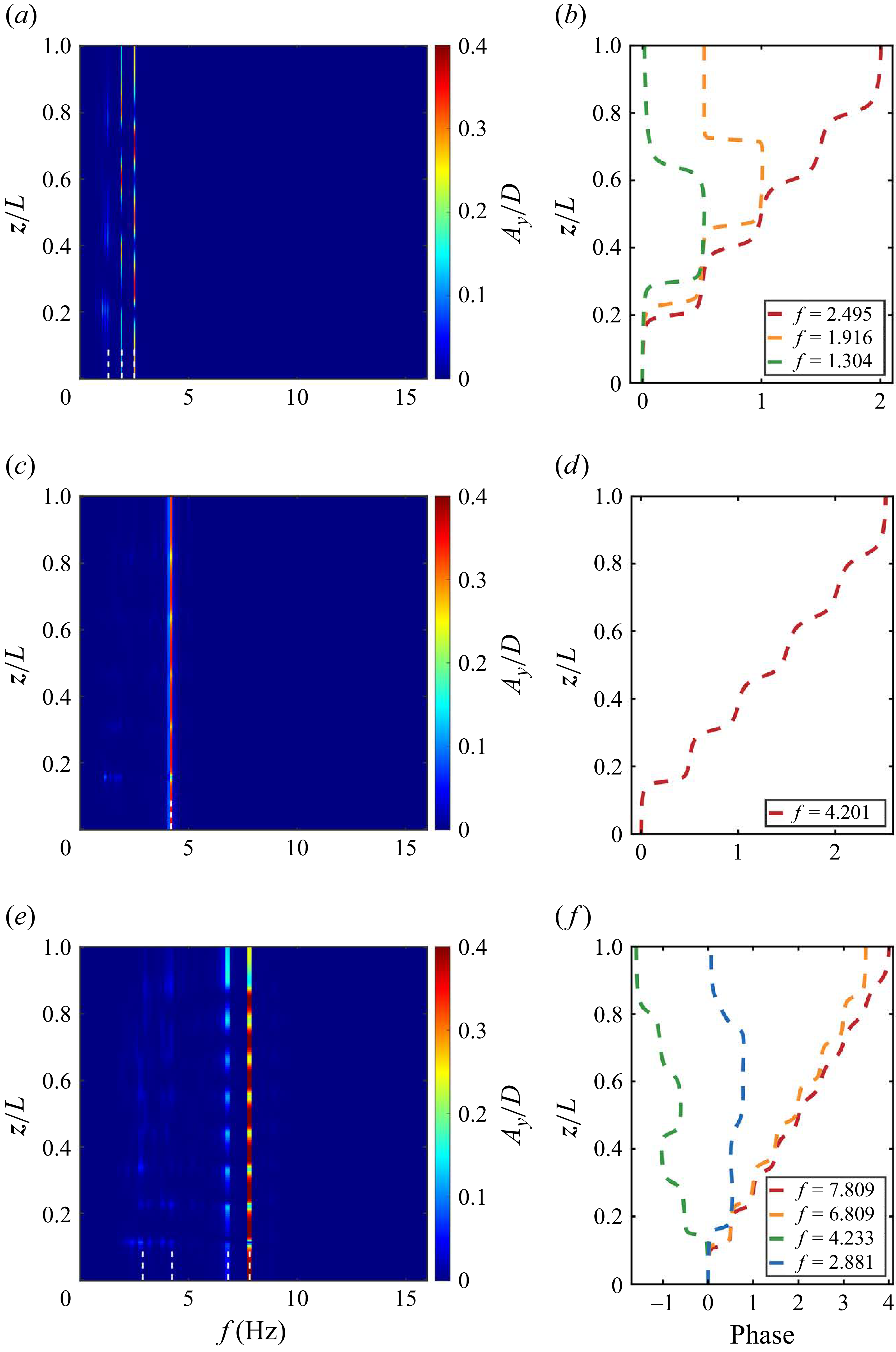
Subsequently, spectral analyses of the structural displacement responses are performed. The power spectral densities (PSDs) are normalised at each spanwise location by the corresponding displacement variance to eliminate the influence of amplitude on spectral magnitude (Bourguet et al. Reference Bourguet, Karniadakis and Triantafyllou2011a
), as shown in figures 4(a), 4(c) and 4(e). At
 $U_{\infty }=0.38$
ms−1 (within the modal group), a response dominated by a single frequency
 $f=4.201$
Hz is observed along the entire span (figure 4
c), corresponding to a mono-frequency response regime. However, At
 $U_{\infty }=0.20$
ms−1, two comparable response frequencies coexist and compete, accompanied by secondary peaks, leading to a multi-frequency response regime. Multi-frequency response also occurs at
 $U_{\infty }=0.65$
ms−1, where multiple peaks emerge but one is dominant. In this case, the excited frequencies span a broad range of [2.881, 7.807], corresponding to a broadband response, which was first identified by Bourguet et al. (Reference Bourguet, Karniadakis and Triantafyllou2013) for a long flexible cylinder subjected to an exponentially shear flow. Benefiting from the efficiency of the present algorithm, extensive simulations demonstrate that mono-frequency responses consistently occur within modal groups, whereas multi-frequency responses arise in the modal-transition region, as shown in figure 2
 $(b)$
. In the figure, each red dot denotes a frequency component of the displacement response. Within the grey-shaded velocity range, several frequency components coexist, signifying a multi-frequency response. This region aligns precisely with the modal-transition region.
 $(a,c,e)$
Temporal spectral analysis of CF displacement along the CTR span and
 $(b,d,f)$
spanwise evolution of selected temporal mode phase angles at
 $(a,b)$
 $U_{\infty }=0.20$
ms−1,
 $(c,d)$
 $U_{\infty }=0.38$
ms−1 and
 $(e,f)$
 $U_{\infty }=0.65$
ms−1.

Moreover, the spanwise evolution of phase angles exhibits pronounced differences between these two regimes. Following the method of Lucor, Mukundan & Triantafyllou (Reference Ma and Srinil2006), the structure response is expressed as
 $N+1$
temporal Fourier modes
 \begin{equation} A_y(z,t)\approx \sum _{q=-N/2}^{N/2}{a_q^y(z)}\exp {[2\pi if_q t]}=\sum _{q=-N/2}^{N/2}{|a_q^y|(z)\exp {[i(2\pi f_qt+\phi _q^y(z))]}}, \end{equation}
where
 $a_q^y$
are written in terms of its moduli
 $|a_q^y|$
and spatial phase angles
 $\phi _q^y$
, and
 $f_q$
is the frequency associated with the
 $q$
th mode and
 $T_s$
the sampling period, namely
 $f_q=q/T_s$
. figures 4(b), 4(d) and 4(f) show the spanwise distribution of phase angles at several selected frequencies (marked by the white dashed lines in figures 4(a), 4(c) and 4(e)). At
 $U_{\infty }=0.38$
ms−1, the phase angles at the dominant frequency decrease monotonically with decreasing
 $z$
, indicating travelling waves propagating from the high-velocity region (near
 $z/L=1$
) toward the low-velocity region. In contrast, at
 $U_{\infty }=0.20$
and
 $U_{\infty }=0.65$
ms−1, the phase evolution consists of two components: one exhibiting the same monotonic variation as in the mono-frequency case, and another originating from a specific mid-span location and varying toward both ends, as illustrated in figures 4(a) and 4(c). Accordingly, 3.1 can be decomposed into two parts as
 \begin{equation} A_y(z,t)=\!\!\sum _{q=-N_m/2}^{N_m/2}{|a_q^y|(z)\exp {[i(2\pi f_qt\!+\!\phi _q^y(z))]}} \!+\! \!\sum _{q=-N_l/2}^{N_l/2}{|a_q^y|(z)\exp {[i(2\pi f_qt\!+\!\phi _q^y(z))]}}, \end{equation}
where
 $N_m$
and
 $N_l=N-N_m$
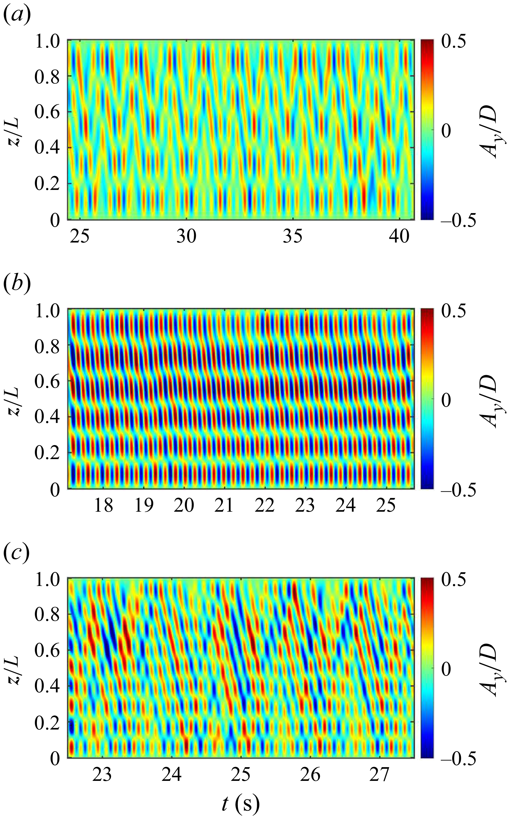
denote the sets of monotonic and non-monotonic phase components, respectively. The implications of these distinct behaviours are revealed in figure 5, which shows the temporal evolution of CF displacement along the CTR span at different incoming velocities. In the mono-frequency response regime, the first term in (3.2) dominates, producing a stable downstream propagation of response from the high normal-velocity region at the top to the low normal-velocity region at the bottom, consistent with the monotonic phase variation of the dominant frequency (figure 5
b). In contrast, in the multi-frequency regime, both terms contribute significantly, leading to pronounced travelling-wave reflection – the response energy initially propagates downward before being reflected upward from the bottom end, as shown in figures 5(a) and 5(c).
The temporal evolution of CF displacement along the CTR span at
 $(a)$
 $U_{\infty }=0.20$
ms−1,
 $(b)$
 $U_{\infty }=0.38$
ms−1 and
 $(c)$
 $U_{\infty }=0.65$
ms−1.

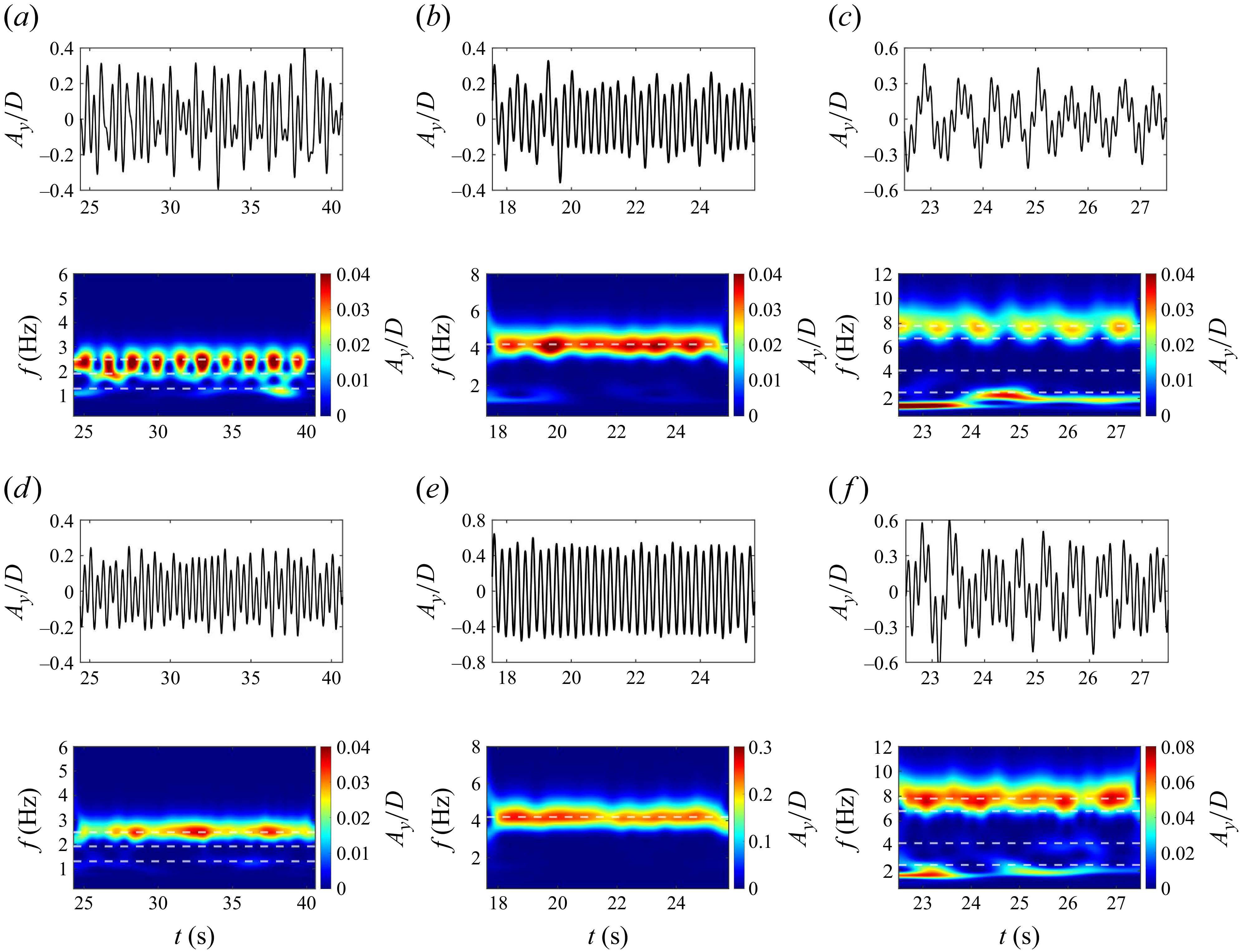
Another important question is whether the multi-frequency response observed in the modal-transition region is a sustained multi-frequency state, or it is instantaneously mono-frequency with a shifting frequency in time. To address this, wavelet analyses were conducted on CF displacement signals at two spanwise locations,
 $(a,b,c), z/L=0.134$
and
 $(d,e,f), z/L=0.721$
, with the resulting time–frequency spectra shown in figure 6. In each case, the upper part presents the displacement signals within the selected time interval, and the lower part displays the corresponding time–frequency spectra. In the mono-frequency regime (
 $U_{\infty }=0.38$
ms−1), the dominant frequency remains nearly constant, closely matching the peak identified in figure 4
 $(c)$
, as indicated by the dashed line, and this behaviour is consistent across both spanwise positions (figures 6
b and 6
c). By contrast, in the multi-frequency regimes (
 $U_{\infty }=0.20$
and
 $0.65$
ms−1), the vibration frequency exhibits pronounced temporal and spatial variability. In these cases, the structural response is instantaneously dominated by a single frequency that drifts regularly between the predominant peaks, producing the cellular pattern evident in figures 6(a) and 6(c). Thus, the multi-frequency responses observed in the spectra can be interpreted as a sequence of ‘instantaneous mono-frequency’ states, a behaviour first reported by Bourguet et al. (Reference Bourguet, Karniadakis and Triantafyllou2011a
) in the VIV of flexible cylinders in shear flows. Additionally, the multi-frequency response has also been observed by Seyed-Aghazadeh et al. (Reference Seyed-Aghazadeh, Budz and Modarres-Sadeghi2021) and Zhu et al. (Reference Zhu, Lin and Gao2021), who respectively associated it with intermittent vortex-shedding pattern and modal switching phenomena. The broadband character is particularly pronounced at
 $U_{\infty }=0.65$
ms−1, where the increased inflow velocity amplifies the difference between the maximum and minimum local velocities (Bourguet et al. Reference Bourguet, Karniadakis and Triantafyllou2013). Spatial variability is also a key feature of the multi-frequency regime: for example, clear temporal frequency switching is evident in figures 6(a) and 6(c), whereas the response at
 $z/L=0.721$
(figures 6
d and 6
f) remains nearly constant.
Selected CF displacement time series and corresponding frequency spectra at
 $(a,b,c)$
 $z/L=0.134$
and
 $(d,e,f)$
 $z/L=0.721$
, under
 $(a,d)$
 $U_{\infty }=0.20$
ms−1,
 $(b,e)$
 $U_{\infty }=0.38$
ms−1 and
 $(c,f)$
 $U_{\infty }=0.65$
ms−1. Dashed lines indicate the predominant frequencies identified in figure 4.

In summary, two distinct response regimes are identified in the structure response of CTRs. The first is a mono-frequency regime, dominated by a single vibration frequency, where the phase angle varies monotonically along the span and the temporal evolution of displacement is steadily transferred from the high normal-velocity region to the low normal-velocity region. The second is a multi-frequency regime, characterised by the coexistence of several dominant frequencies. This overall character can be interpreted as the superposition of several temporally instantaneous mono-frequencies, whose superposed propagation of phase angle characteristics give rise to travelling-wave reflection of the temporal evolution. Leveraging the efficiency of the present algorithm, the underlying connection of these regimes can be generalised: the mono-frequency response is typically associated with local lock-in within a modal group, whereas the multi-frequency response emerges in the modal-transition region. Despite these differences, a mixed standing–travelling-wave pattern consistently arises as a unifying feature across all cases.
3.2. Fluid–structure interaction characteristics
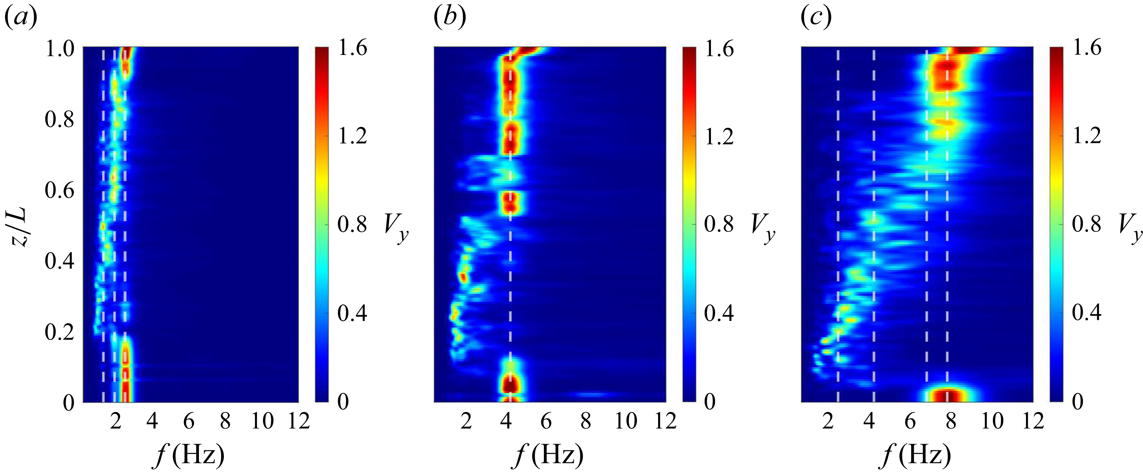
Owing to the geometric configuration of CTRs, additional effects such as flow–curvature interactions can induce spanwise variations in vortex-shedding patterns and frequencies, even under uniform incoming flow. The questions that arise are how do vortex-shedding frequencies vary along the span under mono-frequency and multi-frequency response regimes, and in what ways do these behaviours differ? To address this, the PSD of the CF velocity component of flow,
 $V_{y}$
, is plotted along the span for three inflow velocities in figure 7, where the white dashed lines indicate the predominant structural vibration frequencies identified in figure 4. Three characteristic spanwise regions are distinguished in all cases: two lock-in regions occur in both the high normal-velocity zone near the top of the CTRs and the low normal-velocity zone near the bottom, where the vortex-shedding frequency coincides with the structural vibration frequency. By contrast, the mid-span corresponds to a non-lock-in region, characterised by a mismatch between the vortex shedding and structural vibration frequencies. This behaviour is different from the findings of Bourguet et al. (Reference Bourguet, Karniadakis and Triantafyllou2011a
,
Reference Bourguet, Modarres-Sadeghi, Karniadakis and Triantafylloub
) for flexible risers in linear shear flows, where only two regions were identified: a lock-in region confined to the high-velocity zone and a non-lock-in region elsewhere.
Temporal spectral analysis of the CF component of the flow velocity along a spanwise line in the wake at
 $(a)$
 $U_{\infty }=0.20$
ms−1,
 $(b)$
 $U_{\infty }=0.38$
ms−1 and
 $(c)$
 $U_{\infty }=0.65$
ms−1. The white dashed lines indicate the frequencies identified in figure 4.

Concretely, in the mono-frequency regime at
 $U_{\infty }=0.38$
ms−1, the lock-in region is locked to a single dominant frequency. By contrast, in the multi-frequency regimes at
 $U_{\infty }=0.20$
and
 $U_{\infty }=0.65$
ms−1, the lock-in no longer occurs with a single global frequency; instead, different spanwise locations synchronise with different dominant frequencies, a phenomenon can be regarded as ‘local mono-frequency lock-in’. For instance, at
 $U_{\infty }=0.20$
ms−1, the segment
 $z/L \in [0.915,1]$
locks onto the dominant frequency
 $f=2.495$
Hz, whereas
 $z/L \in [0.570,0.915]$
locks onto
 $f=1.916$
Hz. This behaviour is analogous to the ‘distributed lock-in’ reported by Bourguet et al. (Reference Bourguet, Karniadakis and Triantafyllou2013) for flexible risers in exponential shear flows. Moreover, in the non-lock-in region, the shedding frequency decreases systematically with decreasing
 $z$
, consistent with the reduction of the local Strouhal-based frequency along the span, and exhibits a cellular pattern in which spanwise regions of nearly constant shedding frequency are separated by sharp discontinuities (Bourguet et al. Reference Bourguet, Karniadakis and Triantafyllou2011a
).
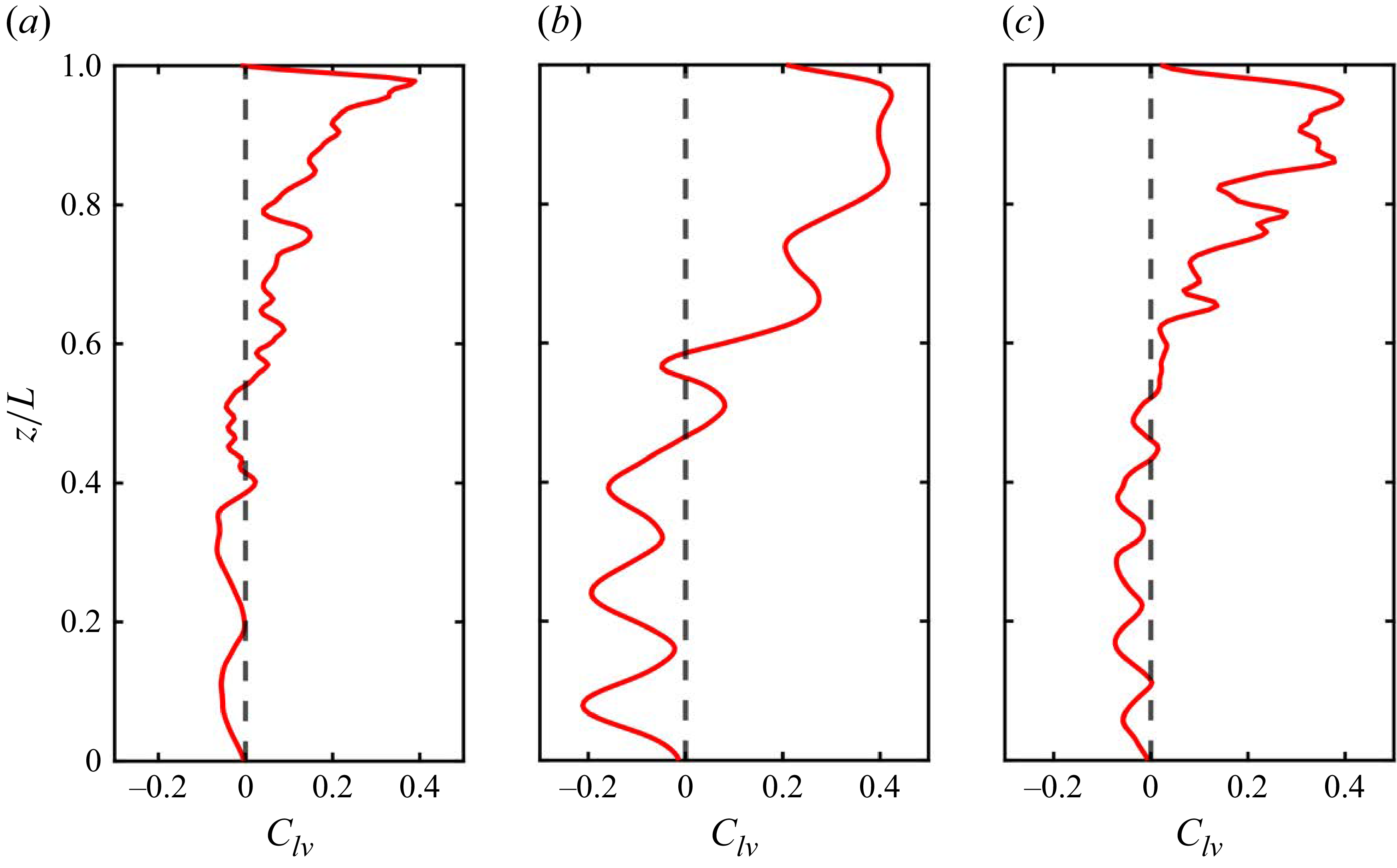
To further elucidate the characteristics of FSI, we examine how the energy transfer between fluid and structure varies across the span of the CTRs. Lock-in is closely associated with this exchange, which constitutes the core mechanism of VIV. Accordingly, the spanwise evolution of the energy transfer parameter,
 $C_{lv}$
, is analysed at three different incoming velocities, as shown in figure 8. The parameter
 $C_{lv}$
is defined as the time-averaged value of the force coefficient component in phase with the structural velocity as
 \begin{equation} C_{lv}(z)= \frac {\frac {1}{T_s} \int _{T_s} (C_l(z,t)V_{s_y}(z,t))\text{d}t}{\sqrt {\frac {1}{T_s}\int _{T_s} V_{s_y}^2(z,t)\text{d}t}}, \end{equation}
where
 $C_l(z,t)$
and
 $V_{s_y}(z,t)$
denote the lift coefficient and the CF structural velocity at different spanwise locations, respectively, while
 $T_s$
represents the selected time series. A positive
 $C_{lv}$
corresponds to energy transfer from the fluid to the structure (flow-induced excitation), whereas a negative
 $C_{lv}$
indicates energy transfer from the structure back to the fluid (damping by the flow).
As shown in figure 8, the spanwise distribution of
 $C_{lv}$
can be divided into two regions: a fluid-excitation region, where
 $C_{lv}\gt 0$
and the structure is excited by the flow, which largely coincides with the top lock-in region at higher normal velocities; and a fluid-damping region, where
 $C_{lv}\lt 0$
and the structure is damped by the flow, which primarily overlaps with the non-lock-in region and the bottom lock-in region at lower normal velocities. The overall trend of
 $C_{lv}$
remains consistent across the three incoming velocities, except that, under mono-frequency response (
 $U_{\infty }=0.38$
ms−1), the variation of
 $C_{lv}$
is relatively smooth, whereas under multi-frequency responses (
 $U_{\infty }=0.20,0.65$
ms−1), the variation becomes more pronounced, particularly within the fluid-excitation region.
The spanwise evolution of the fluid–structure energy transfer parameter
 $C_{lv}$
at
 $(a)$
 $U_{\infty }=0.20$
ms−1,
 $(b)$
 $U_{\infty }=0.38$
ms−1 and
 $(c)$
 $U_{\infty }=0.65$
ms−1.

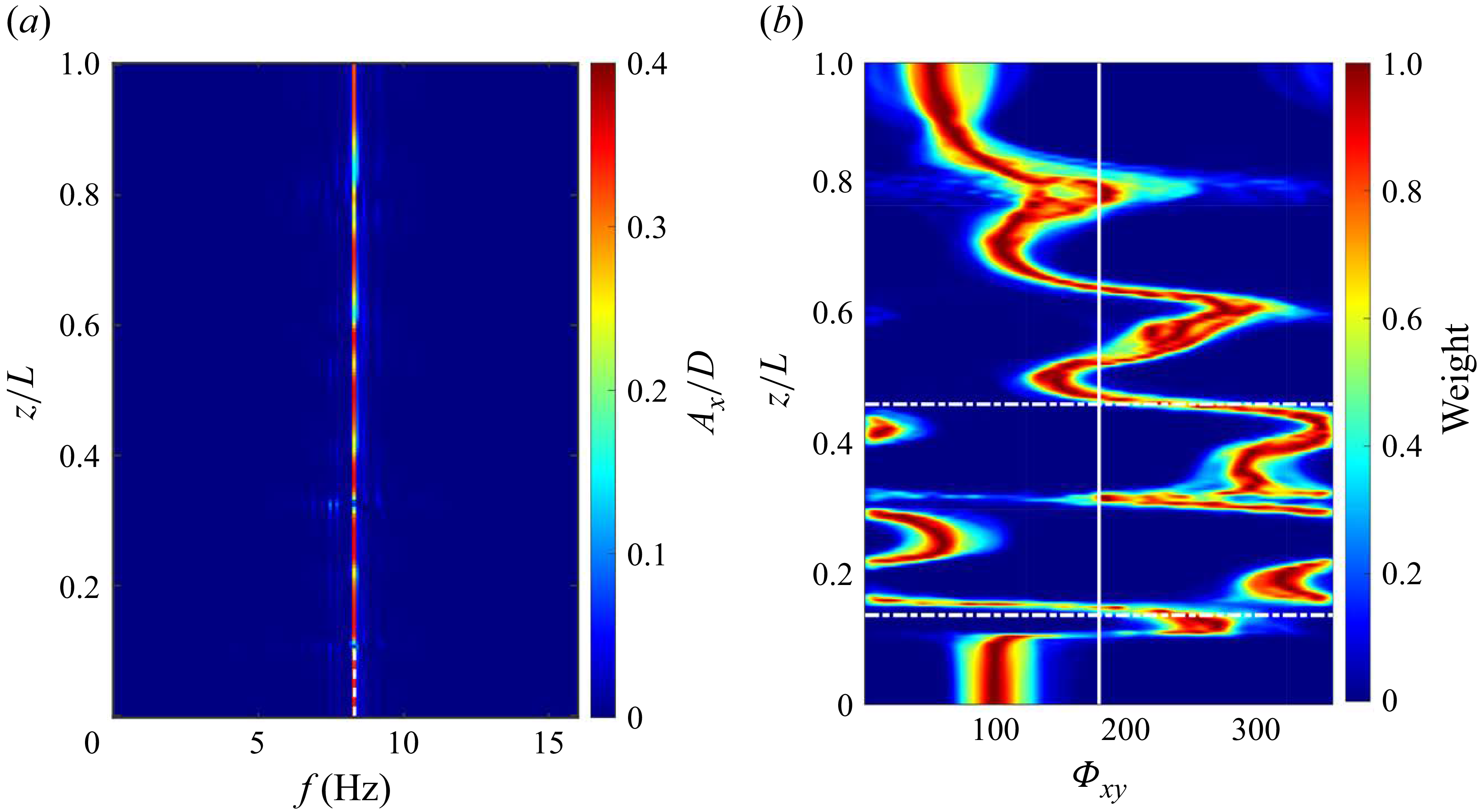
 $(a)$
Temporal spectral analysis of IL displacement along the CTR span and
 $(b)$
spanwise evolution of the histogram of phase difference between the IL and CF displacements
 $\varPhi _{xy}$
at
 $U_{\infty }=0.38$
ms−1.

Moreover, the synchronisation between the IL and CF displacements along the span is shown to be related to the nature of the fluid–structure energy transfer (Dahl et al. Reference Dahl, Hover, Triantafyllou, Dong and Karniadakis2007, Reference Dahl, Hover, Triantafyllou and Oakley2010; Bourguet et al. Reference Bourguet, Karniadakis and Triantafyllou2011a
,
Reference Bourguet, Modarres-Sadeghi, Karniadakis and Triantafylloub
). Therefore, the instantaneous phase of the IL and CF vibrations,
 $\phi _x$
and
 $\phi _y$
, are evaluated using the Hilbert transform to observe their spanwise distribution. Following the approach proposed by Huera-Huarte & Bearman (Reference Huera-Huarte and Bearman2009b
), the phase difference
 $\varPhi _{xy}$
is defined as
 \begin{equation} \varPhi _{xy}=[p\phi _x-q\phi _y, \text{mod} 360^{\circ }], \end{equation}
where
 $p$
and
 $q$
are two integers representing the synchronisation order. To determine these parameters, the spectral analysis of the IL displacement responses was performed at a representative incoming velocity
 $U_{\infty }=0.38$
ms−1, as shown in figure 9
 $(a)$
. In this case, the response is dominated by a single frequency
 $f_x=8.303$
Hz, which is approximately twice the CF vibration frequency
 $f_y=4.201$
Hz as shown in figure 4
 $(c)$
. Accordingly, the couple
 $(p, q) = (1, 2)$
is adopted.
To quantify the predominant phase difference along the span, histograms of
 $\varPhi _{xy}$
are evaluated from the corresponding time series. Figure 9
 $(b)$
presents the relative weights of the phase difference angles along the CTR span at
 $U_{\infty }=0.38$
ms−1, normalised by the maximum weight. According to previous studies (Bourguet et al. Reference Bourguet, Karniadakis and Triantafyllou2011a
,
Reference Bourguet, Modarres-Sadeghi, Karniadakis and Triantafylloub
), values of
 $\varPhi _{xy}$
within
 $0^{\circ }-180^{\circ }$
 $(180^{\circ }-360^{\circ })$
correspond to trajectories where the cylinder moves upstream (downstream) when reaching the CF oscillation maxima. These two types of trajectories are referred to as counter-clockwise (CC) and clockwise (C), respectively. In figure 9
 $(b)$
, the vertical white line indicates the position where
 $\varPhi _{xy}=180^{\circ }$
. Three regions can be distinguished, which are separated by the dashed lines in figure 9
 $(b)$
. For
 $z/L\gt 0.458$
,
 $\varPhi _{xy}$
is generally less than
 $180^{\circ }$
, indicating that CC trajectories dominate this region and correspond to positive energy transfer to the structure. Values slightly exceeding
 $180^{\circ }$
appear near
 $z/L = 0.6$
, which is related to the interruption observed at this location, as shown in figure 8
 $(b)$
. In contrast, C trajectories mainly occur in the range
 $0.139\lt z/L\lt 0.458$
, where the fluid forces are primarily damping. The switching CC–C pattern is altered by the development of mainly travelling waves oriented from high- to low-velocity regions (decreasing z). Moreover, for
 $z/L\lt 0.139$
, the spanwise evolution of the phase angle remains nearly constant, resembling standing-wave behaviour in both the IL and CF directions. In the present of mixed standing–travelling-wave responses,
 $\varPhi _{xy}$
exhibits a zigzaging spanwise pattern, drifting toward higher phase difference angles as z decreases. These results are consistent with the findings reported by Bourguet et al. (Reference Bourguet, Modarres-Sadeghi, Karniadakis and Triantafyllou2011b
).
Based on the spanwise evolution of the lock-in phenomena, fluid–structure energy transfer parameter
 $C_{lv}$
and the phase difference
 $\varPhi _{xy}$
, three distinct regimes are revealed along the span of the CTRs:
-
(i) Flow-induced lock-in regime (F-L regime): for the high normal velocity near the top of the CTRs, the high normal velocity excites the structure vibration and transfers energy from the flow to the structure. In this regime, the vortex-shedding frequency coincides with the structural vibration frequency and the vibration predominantly follows CC trajectories, corresponding to
 $\varPhi _{xy}\lt 180^{\circ }$
and
$C_{lv}\gt 0$
.
-
(ii) Non-lock-in regime (N-L regime): for the medium normal velocity in the middle of the CTRs, the vortex-shedding frequency departs from the vibration frequency, accompanied by the emergence of a discontinuous, cellular pattern. In this regime, the energy transfer parameter
$C_{lv}\lt 0$
and is accompanied by C trajectories. -
(iii) Structural resonance regime (S-R regime): for the low normal velocity in the bottom of the CTRs, the travelling waves from the upper span evolve into standing waves, driving the local structural vibration and the phase difference remains nearly constant. Here, the incoming flow has little influence on vortex shedding, which is instead entrained by the structural motion. As a result, the vortex-shedding frequency once again coincides with the vibration frequency, but
$C_{lv}\lt 0$
, indicating that energy is transferred from the structure back to the flow and the flow damps the vibration.


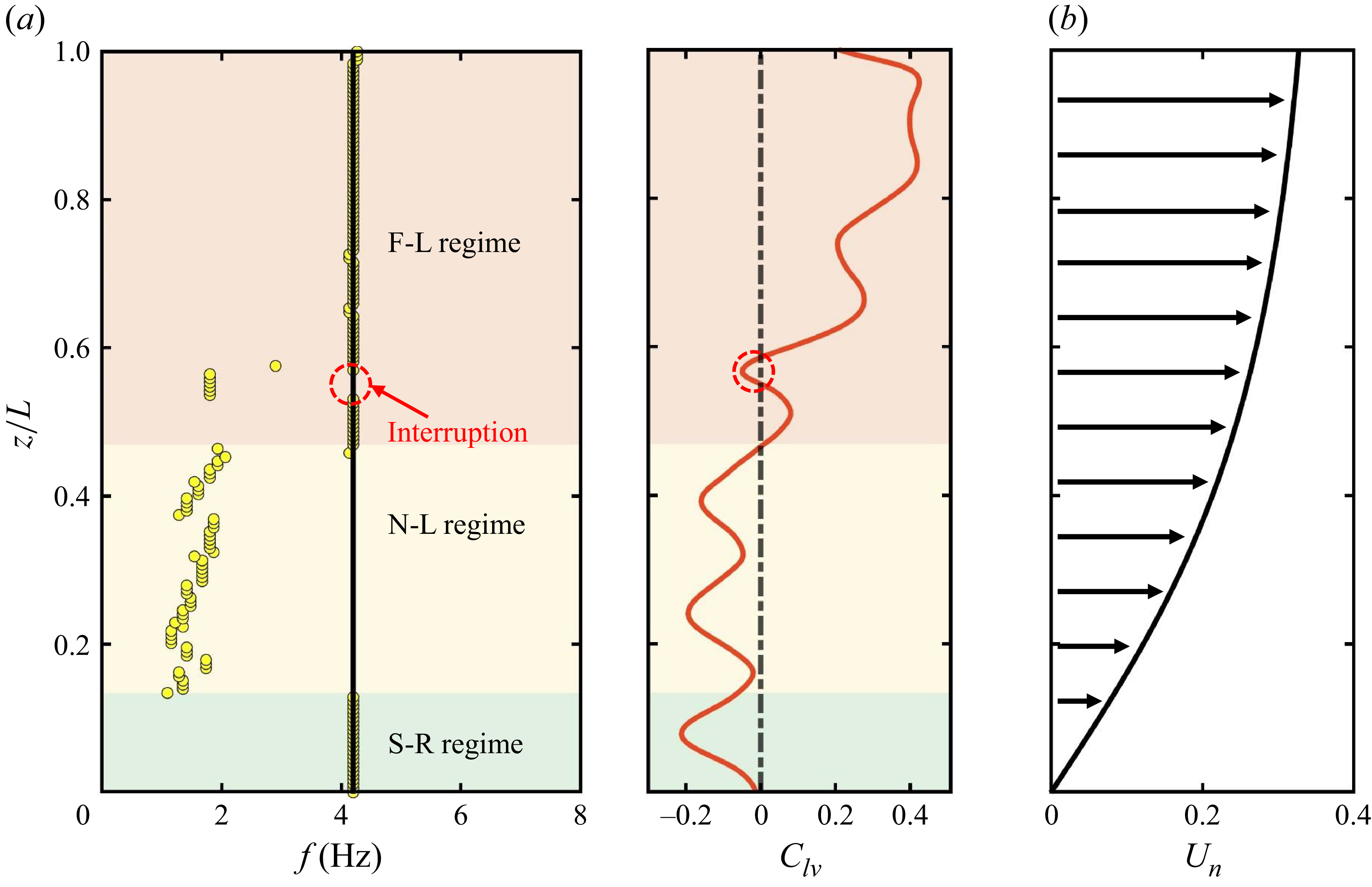
Schematic of the spanwise regimes of the CTRs at
 $U_{\infty }=0.38$
ms−1.
 $(a)$
Spanwise evolution of the vortex-shedding frequency (left) and the fluid–structure energy transfer parameter
 $C_{lv}$
(right), where yellow dots indicate the shedding frequency at each spanwise location and the black line denotes the dominant structural vibration frequency extracted from figure 4(c);
 $(b)$
the normal velocity
 $U_n$
along the CTR span based on the IP. Three spanwise regimes are distinguished by background shading.

Figure 10 illustrates the distribution of the three regimes at the representative incoming velocity of
 $U_{\infty }=0.38$
ms−1. Figure 10
 $(b)$
presents the corresponding normal-velocity profile, derived using the IP. To clarify the transition behaviour, two critical positions are defined:
 $F_c$
, marking the onset of transition from the F-L regime to the N-L regime, and
 $S_c$
, marking the onset of transition from the S-R regime to N-L regime. For example, the interval
 $z/L \in [0.458,1]$
corresponds to the F-L regime, with
 $F_c=0.458$
, while
 $z/L \in [0,0.134]$
corresponds to the S-R regime, with
 $S_c=0.134$
. The remaining interval,
 $z/L \in [0.134,0.458]$
, is therefore identified as the N-L regime, as shown in figure 10
 $(a)$
. These three regions collectively delineate the axial partitioning of the CTR response, providing a clear physical framework for understanding the interplay between flow-induced and structure-induced mechanisms. Notably, within the F–L regime, intermittent interruption occurs, where the vortex-shedding and vibration frequencies deviate with
 $C_{lv}\lt 0$
, as highlighted by the red circle in figure 10
 $(a)$
.
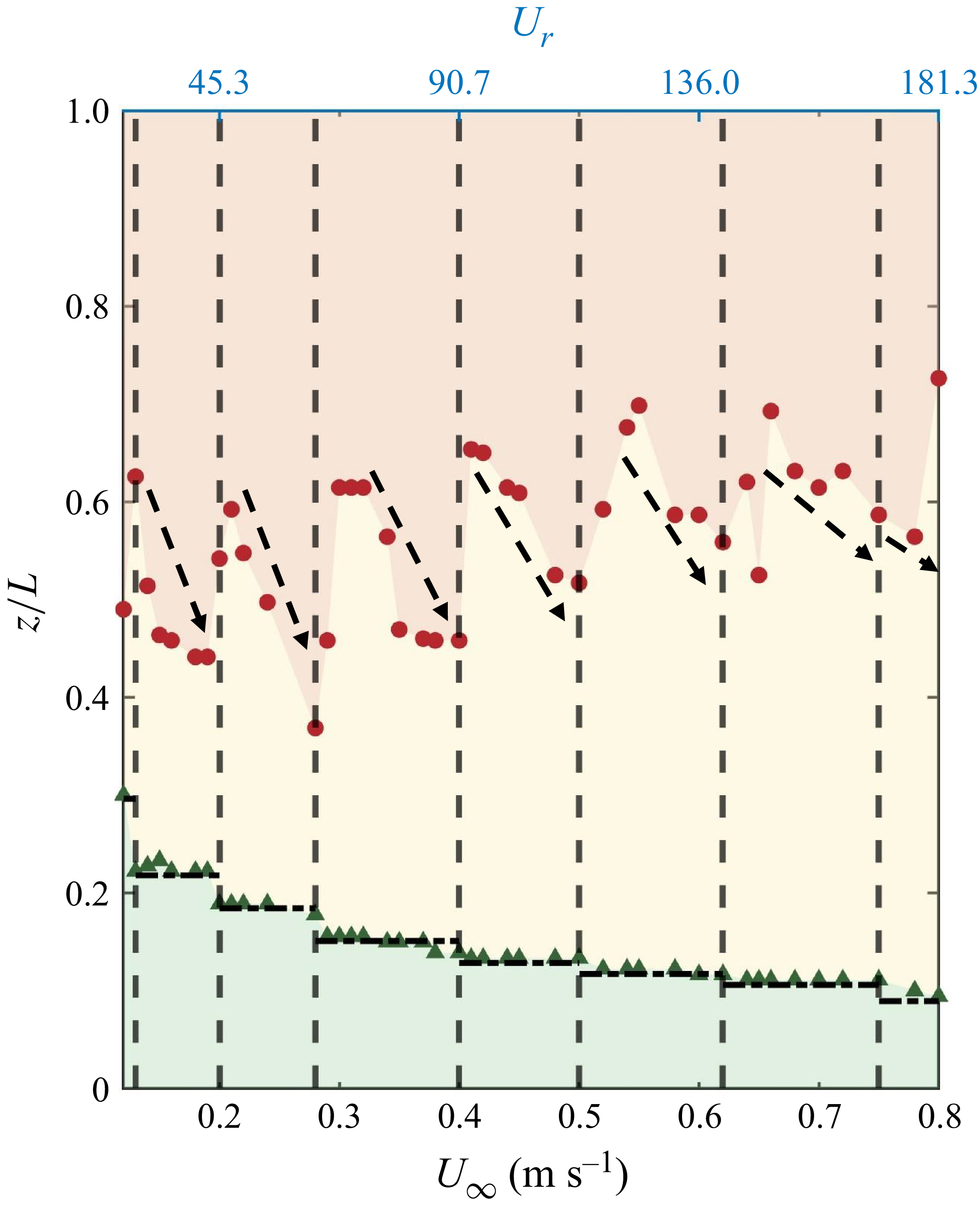
Distribution of spanwise regimes as a function of the incoming velocity
 $U_{\infty }$
ms−1. The vertical dashed line indicates the boundary between different modal groups, as shown in figure 2. The red dots and green triangles denote the locations of
 $F_c$
and
 $S_c$
, respectively.

These findings naturally raise two important questions: How does the incoming velocity modulate the distribution of these regimes, and what physical mechanisms govern their distribution? From an engineering perspective, clarifying the distribution of these regimes is of considerable practical significance, as it enables the formulation of targeted strategies based on the response characteristics of each regime. To address these questions, we investigate a range of incoming velocities, thereby uncovering the intrinsic principles governing the spanwise partitioning of regimes in the next section.
3.3. Modulation of spanwise regimes by incoming velocity
The spatial distributions of these three spanwise regimes under different incoming velocities
 $0.12 \leqslant U_{\infty } \leqslant 0.8$
(corresponding
 $1660 \leqslant Re \leqslant 11067$
) are compared in figure 11, with identical regimes highlighted using consistent background colours for ease of comparison. Within the same modal group (i.e. between any two vertical dashed lines in figure 11(a)), the proportion of the flow-induced lock-in regime increases with
 $U_{\infty }$
. This indicates that a larger portion of the span is subjected to energy transfer from the flow, leading to greater vibration amplitudes. As shown in figure 2
 $(a)$
, the maximum amplitude of the r.m.s.
 $(A_y^{rms}/D)_{max}$
correspondingly increases with
 $U_{\infty }$
within the same modal group. In contrast, the critical position
 $S_c$
remains nearly constant within each modal group but shifts downward with increasing mode number, as indicated by the horizontal black dashed line in figure 11, suggesting that the structural resonance regime is primarily governed by the structural mode number rather than the incoming velocity. The underlying physical mechanism is discussed in detail in § 4.3.
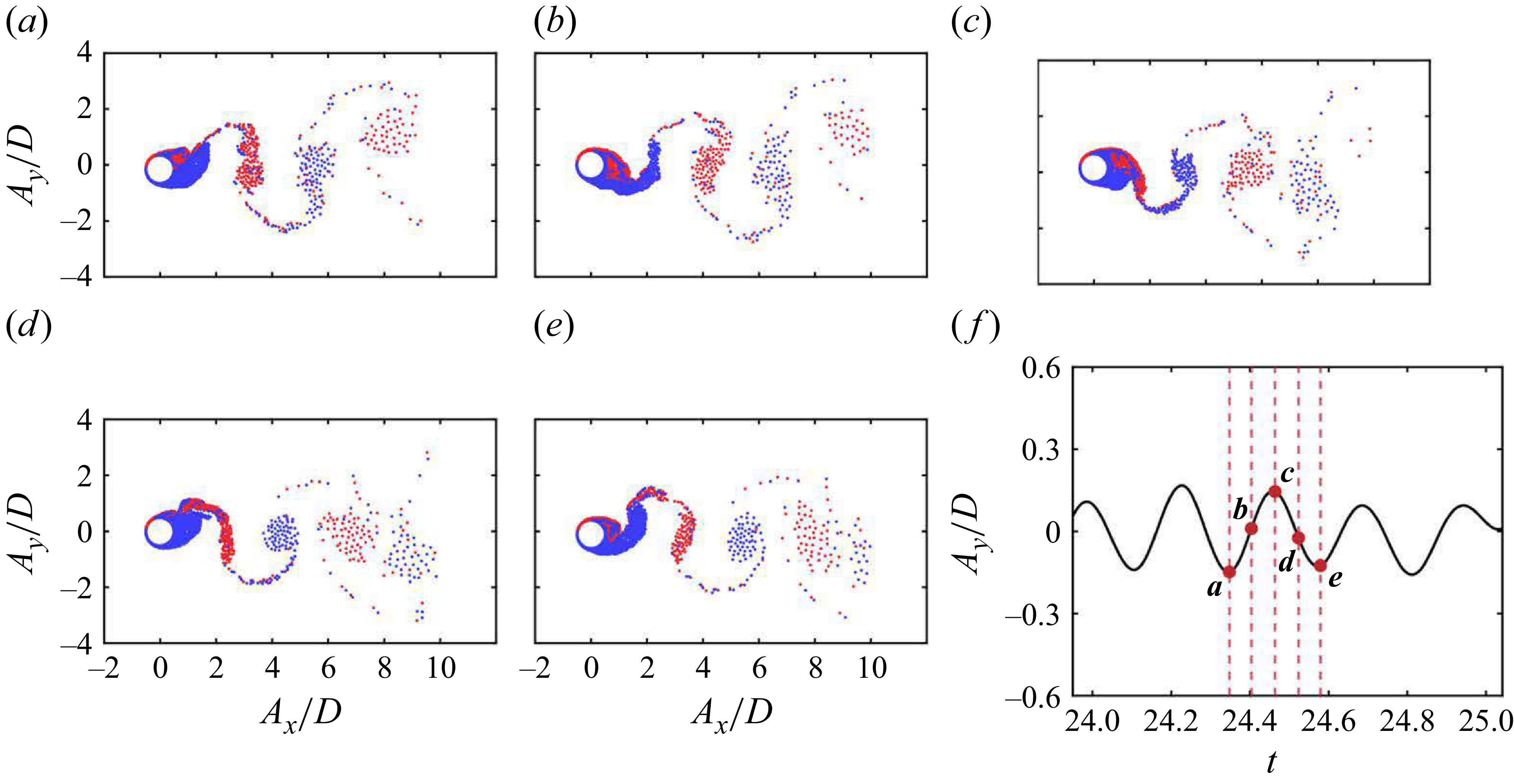
Simulation results of vortices at
 $z/L=0.726$
for
 $U_{\infty }=0.38$
ms−1 and
 $Z_H=7.13$
over one period of CF oscillation:
 $(a{-}e)$
instantaneous field of vortices;
 $(f)$
time trace of the cylinder CF motion. The red circle highlights the corresponding time from
 $(a)$
to
 $(e)$
.

By contrast, the physical mechanism underlying the flow-induced lock-in regime remains unclear. This suggests that varying the incoming velocity alone is insufficient to elucidate its origin, and that additional influencing factors must be considered. Among these, the initial geometric configuration of the CTRs warrants particular attention, as changes in geometry can significantly modify both the normal-velocity component acting on the structure and the axial tension, thereby altering the spatial distribution of the three spanwise regimes. To address this question, we conduct simulations of CTRs with different initial configurations in § 4.
Simulation results of vortices at
 $z/L=0.977$
for
 $U_{\infty }=0.38$
ms−1 and
 $Z_H=7.13$
over one period of CF oscillation:
 $(a{-}e)$
instantaneous field of vortices;
 $(f)$
time trace of the cylinder CF motion. The red circle highlights the corresponding time from
 $(a)$
to
 $(e)$
.

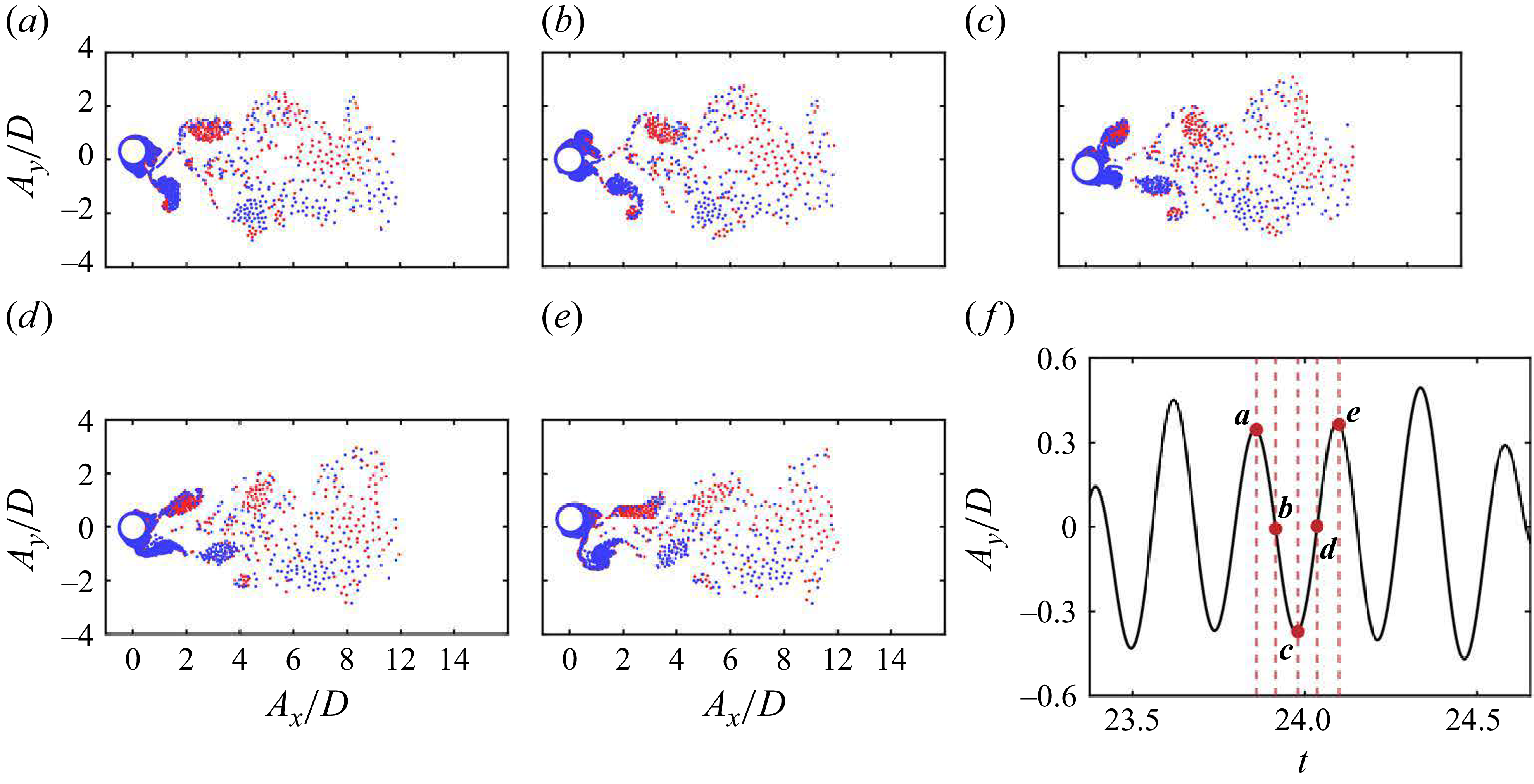
Simulation results of vortices at
 $z/L=0.419$
for
 $U_{\infty }=0.38$
ms−1 and
 $Z_H=7.13$
over one period of CF oscillation:
 $(a{-}e)$
instantaneous field of vortices;
 $(f)$
time trace of the cylinder CF motion. The red circle highlights the corresponding time from
 $(a)$
to
 $(e)$
.

3.4. Wake patterns under different spanwise regime
Finally, the wake patterns corresponding to different spanwise regimes are examined. Similar to the findings of Techet, Hover & Triantafyllow (Reference Vandiver1998), Flemming & Williamson (Reference Flemming and Williamson2005), Huera-Huarte & Bearman (Reference Huera-Huarte and Bearman2009b
) and Seyed-Aghazadeh et al. (Reference Seyed-Aghazadeh, Budz and Modarres-Sadeghi2021), who reported the coexistence of multiple shedding patterns along the span of flexible cylinders, four representative patterns are identified for the CTRs. For example, the shedding patterns at different spanwise regimes at
 $U_{\infty }=0.38$
ms−1 and
 $Z_H=7.13$
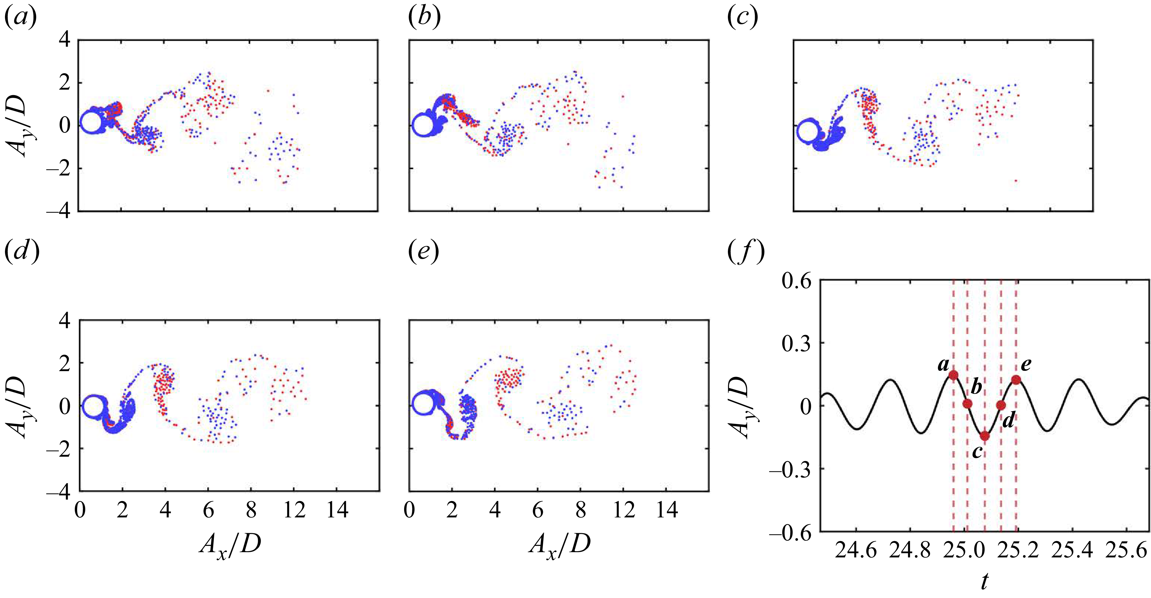
are shown in figures 12, 13, 14 and 15. In subfigures
 $(a{-}e)$
, positive (CC) and negative (C) vorticities are indicated by blue and red dots, respectively, while subfigure
 $(f)$
shows the corresponding CF motion trace, with red circles denoting the time of the snapshots. It should be noted that the wake vortices appear increasingly diffuse with downstream distance due to the vortex-merging criterion introduced in § 2.1. This effect is enhanced in the far field, leading to sparser vortex elements, but it does not affect the identification of the overall shedding pattern.
Simulation results of vortices at
 $z/L=0.112$
for
 $U_{\infty }=0.38$
ms−1 and
 $Z_H=7.13$
over one period of CF oscillation:
 $(a{-}e)$
instantaneous field of vortices;
 $(f)$
time trace of the cylinder CF motion. The red circle highlights the corresponding time from
 $(a)$
to
 $(e)$
.

In the flow-induced lock-in regime, the wake is generally dominated by a shedding mode of ‘2P’, as exemplified in figure 12 at
 $z/L=0.726$
. The evolution over one vibration cycle is shown in subfigures
 $(a{-}e)$
as: at the bottom of the cylinder trajectory (subfigure
 $a$
), a vortex pair (one positive and one negative) is about to detach from the cylinder rear, while an additional positive vortex develops in the upper shear layer and a negative vortex develops in the lower shear layer, connected to the soon-to-detach negative vortex. As the cylinder moves upward (subfigure
 $b$
), the positive vortex stretches across the rear together with the lower negative vortex, which subsequently splits into two. When the cylinder reaches the top of its oscillation (subfigure
 $c$
), another vortex pair detaches from the near, while a new negative vortex forms in the lower shear layer and a positive vortex in the upper shear layer, with the latter connected to the newly detached positive vortex. During the downward motion in the second half-cycle (subfigure
 $d$
), the lower negative vortex extends across the cylinder near field while the upper positive vortex separates from the detached one. Finally, in subfigure
 $(e)$
, the lower vortex detaches from the wake, completing a cycle that repeats the process shown in subfigure
 $(a)$
. Furthermore, within this regime, occasional occurrences of a ‘2S’ shedding pattern are observed at certain locations, as exemplified in figure 13 at
 $z/L=0.997$
. Unlike the ‘2P’ mode, the ‘2S’ pattern is characterised by the regular shedding of a single vortex pair – one positive and one negative – during each oscillation cycle.
In the non-lock-in regime, the wake is mostly dominated by a 2S-like shedding pattern, occasionally interspersed with irregular or intermittent modes. Compared with the classical ‘2S’ mode, the wake is more disordered and the vortex shedding less regular; nevertheless, it consistently exhibits the shedding of one positive and one negative vortex within each oscillation cycle. An illustrative example is shown in figure 14 at
 $z/L=0.419$
. The evolution proceeds as follows: at the top of the cylinder trajectory (subfigure
 $a$
), a negative vortex sheds from the cylinder wake, while a positive vortex and a negative vortex simultaneously begin to form in the upper and lower shear layers, respectively. As the cylinder moves downward (subfigure
 $b$
), both vortices extend progressively on either side of the wake. When the cylinder reaches the bottom of its oscillation (subfigure
 $c$
), the upper positive vortex begins to shed, whereas the lower negative vortex continues to extend. During the upward motion in the second half-cycle (subfigure
 $d,e$
), the lower negative vortex gradually detaches, and new vortices form in the shear layers on both sides of the cylinder, thereby completing a cycle that repeats the process initiated in subfigure
 $(a)$
.
In the structural resonance regime, the shedding mode is predominantly characterised by the ‘P+S’ mode, in which one vortex pair and one single vortex are released from opposite sides of the cylinder within one period of CF vibration. A representative case is shown in figure 15 at
 $z/L=0.112$
. At the top of the cylinder trajectory (subfigure
 $a$
), a positive vortex is about to detach from the cylinder rear, while a negative vortex begins to form in the lower shear layer. As the cylinder moves downward (subfigure
 $b$
), the positive vortex gradually detaches, accompanied by the progressive extension of the lower negative vortex. When the cylinder reaches the bottom of its oscillation (subfigure
 $c$
), the lower negative vortex, together with a positive vortex, simultaneously sheds and grows, a process that continues through subfigure
 $(d)$
. Finally, in subfigure
 $(e)$
, a complete vortex pair detaches from the rear, while a new positive vortex develops in the upper shear layer, thereby completing a cycle that repeats the process shown in subfigure
 $(a)$
. Notably, in this regime, the normal velocity becomes sufficiently small that the vortices convect much more slowly compared with the other regimes.
In summary, distinct dominant shedding modes are observed across different spanwise response regimes. In the flow-induced lock-in regime, the wake is primarily governed by the ‘2P’ mode, with occasional occurrences of the ‘2S’ mode. In the non-lock-in regime, the wake exhibits irregular or intermittent patterns, with a ‘2S-like’ mode occasionally identified, consistent with the findings of Bourguet et al. (Reference Bourguet, Karniadakis and Triantafyllou2011a
). In the structure-reduced lock-in regime, the wake is predominantly characterised by the ‘P+S’ mode. These behaviours persist across all simulations in the present study and agree with the experimental results of Zhu et al. (Reference Zhu, Lin and Yao2019a
), who attributed the differences in wake patterns to phase jumps of approximately
 $180^\circ$
.
4. Vortex-induced vibration response of the CTRs under different initial geometric configurations
This section examines the role of different initial geometric configurations in shaping the VIVs of CTRs, with particular attention to their modulation of the spanwise distribution among the three response regimes. Section 4.1 first characterises the spanwise VIV responses through statistical and spectral analyses (in analogy to § 3.1), together with an assessment of lock-in occurrence and the associated fluid–structure energy transfer (as in § 3.2). The modulation of these spanwise regimes by the initial configuration is then analysed in § 4.2. Finally, § 4.3 elucidates the underlying physical mechanisms governing the sensitivity of the spanwise regimes to variations in both the incoming velocity and the initial geometry.
4.1. The spanwise VIV response characteristics
In present work, the initial configuration is varied by adjusting the vertical height
 $Z_H$
of the CTRs, as described in § 2.3. We investigate the different geometric configurations with
 $Z_H$
ranging from 4.13 to 11.13 at a fixed incoming velocity of
 $U_\infty =0.38$
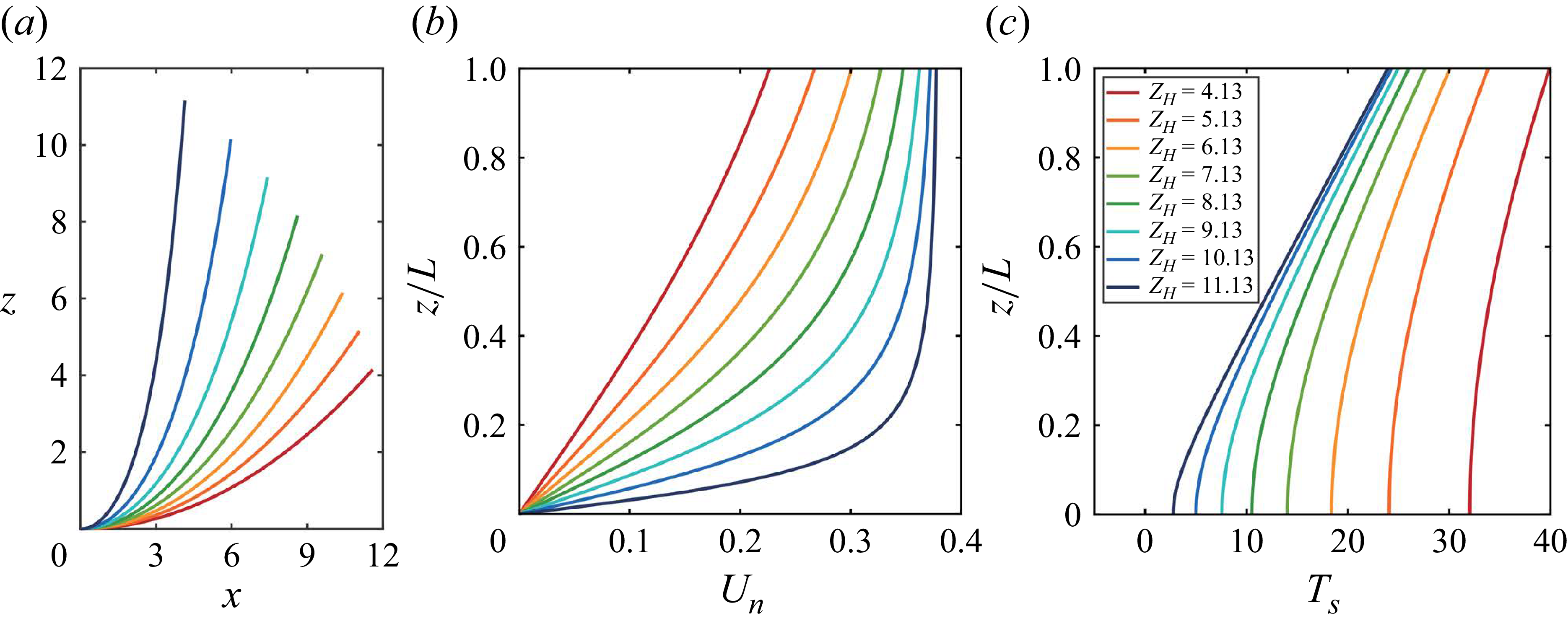
, with the corresponding initial geometries shown in figure 16
 $(a)$
. The initial geometric configuration significantly affects both the normal-velocity component
 $U_n$
acting on the structure and the axial tension
 $T_s$
within the system, as shown in figures 16
 $(b)$
and 16
 $(c)$
, respectively. As
 $Z_H$
increases, the CTR adopts a more vertical configuration and the normal velocity
 $U_n$
increases. The variation of
 $U_n$
becomes smoother near the top but steeper toward the bottom. At the same time, the overall axial tension decreases, while the contrast between its maximum and minimum values becomes more pronounced.
 $(a)$
The initial geometric configuration with different vertical heights
 $Z_H$
;
 $(b)$
normal-velocity component
 $U_n$
ms−1 and
 $(c)$
axial tension
 $T_s$
N alone the CTR span under different
 $Z_H$
at
 $U_{\infty }=0.38$
ms−1.

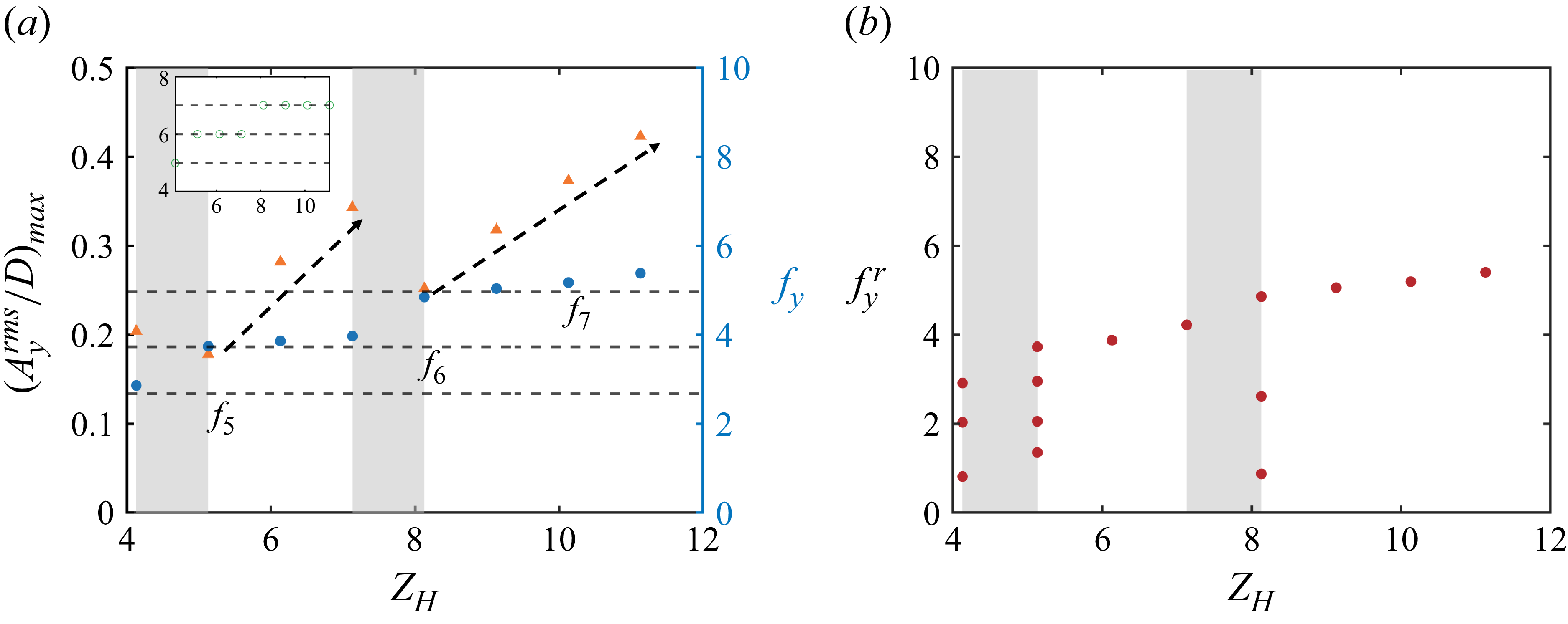
The modal-group switching phenomenon is likewise observed across different vertical heights, as shown in figure 17
 $(a)$
. With increasing
 $Z_H$
, both the number of excited vibration modes and the dominant response frequency rise, transitioning from a fifth-order response at
 $Z_H=4.13$
to a seventh-order response at
 $Z_H=11.13$
. Within each modal group,
 $(A_y^{rms}/D)_{max}$
increases monotonically, consistent with the trend observed under varying incoming velocities (figure 2). As shown in figure 17
 $(b)$
, multiple frequency components appear in the structural response within the modal-transition region (grey-shaded region). To further clarify the spanwise characteristics of VIV responses, two representative cases are examined in detail:
 $Z_H=5.13$
, located in the transition region between the fifth and sixth modal groups, and
 $Z_H=10.13$
, situated within the seventh modal group.
 $(a)$
Dominant frequency
 $f_y$
and maximum r.m.s. CF displacement
 $(A_y^{rms}/D)_{max}$
of CTRs as functions of vertical height
 $Z_H$
at
 $U_{\infty }=0.38$
ms−1. The inset shows the corresponding mode number
 $n$
versus
 $Z_H$
.
 $(b)$
Frequencies involved in the structure response
 $f_y^r$
as a function of
 $Z_H$
, with the grey shading indicating the multi-frequency response region.

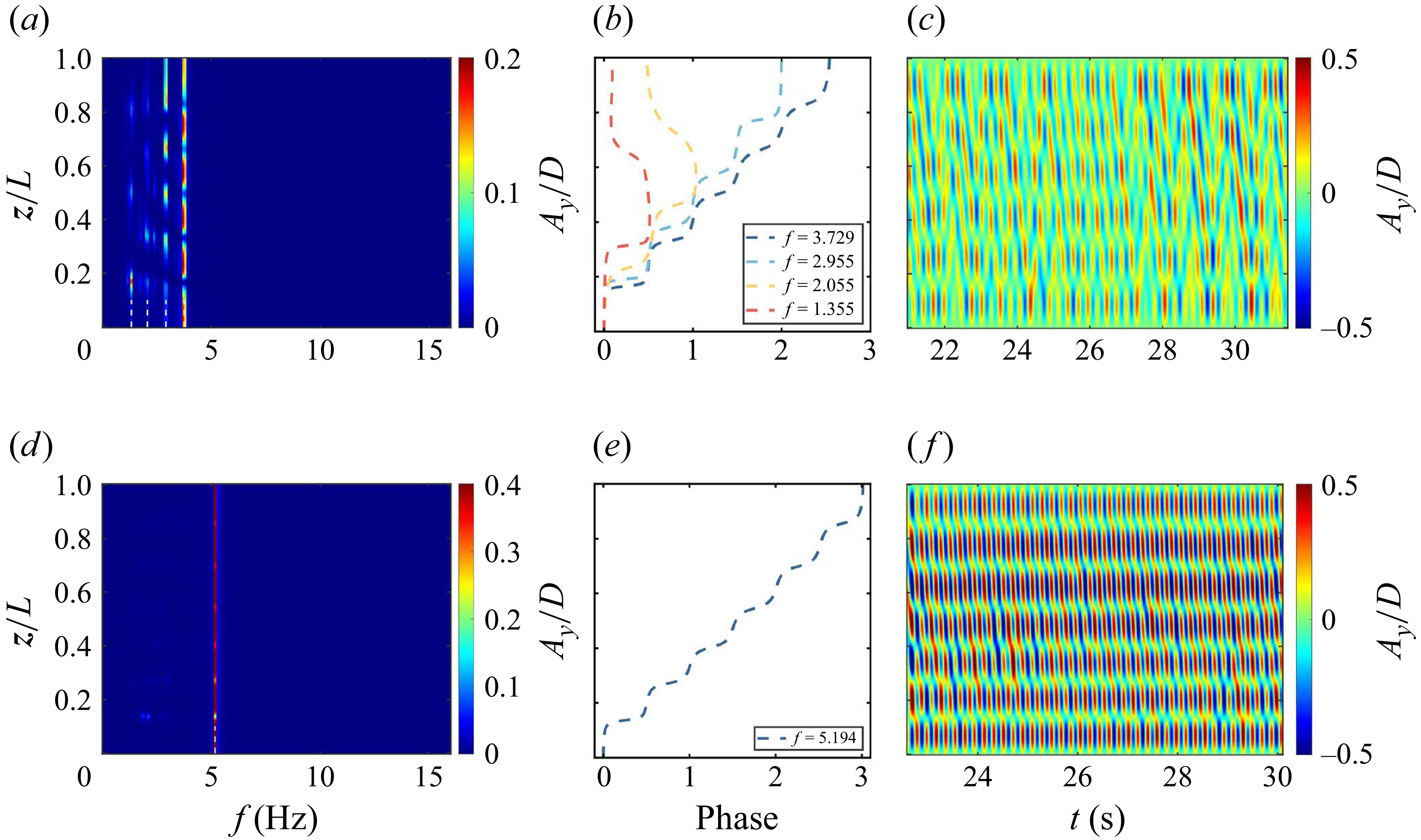
In the modal-transition region (
 $Z_H=5.13$
), the structural displacement response exhibits multi-frequency components, as shown in figure 18
 $(a)$
. Four distinct peaks are identified, corresponding to the 6th, 5th, 4th and 3rd modal contributions, with the 6th mode being dominant. The phase angles of the first two modes increase monotonically with
 $z$
, whereas those of the latter two originate from an intermediate position and propagate toward both ends (figure 18
 $b$
). Consequently, the temporal evolution reveals a pronounced travelling-wave reflection (figure 18
 $c$
). These features are consistent with those observed at
 $U_{\infty }=0.65$
ms−1 in § 3.1. Within the modal group (
 $Z_H=10.13$
), the response exhibits a mono-frequency, as shown in figure 18
 $(d)$
, dominated by a single frequency corresponding to the 7th mode. The associated phase angle increases monotonically with
 $z$
, with no additional components present. As a result, the temporal evolution exhibits a stable downstream propagation, extending from the high normal-velocity region at the top to the low normal-velocity region at the bottom (figures 18
e and 18
f). These features are consistent with the response observed at
 $U_{\infty }=0.38$
ms−1 in § 3.1.
 $(a{,}d)$
Temporal spectral analysis of the CF displacement along the CTR span;
 $(b{,}e)$
spanwise evolution of phase angles for selected frequencies; and
 $(c{,}f)$
temporal evolution of the CF displacement along the CTR span, for
 $(a{-}c)$
 $Z_H=5.13$
and
 $(d{,}e{,}f)$
 $Z_H=10.13$
. All simulations are performed at
 $U_{\infty }=0.38$
ms−1.

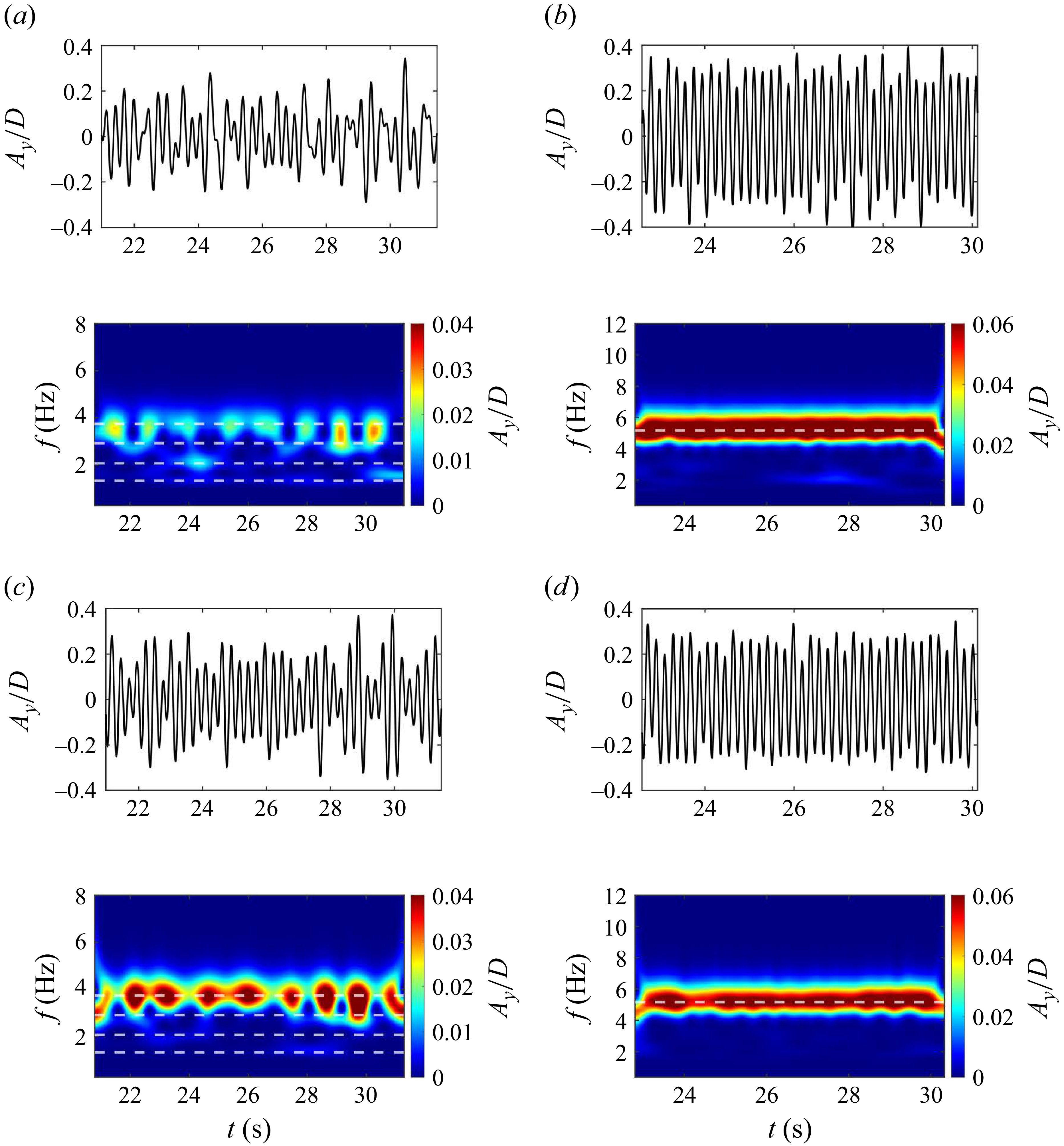
Similarly, figure 19 presents the time–frequency spectra of the CF displacement at two spanwise locations,
 $(a{-}c), z/L=0.134$
and
 $(d{-}f), z/L=0.721$
, for vertical heights
 $Z_H=5.13$
and
 $Z_H=10.13$
. The phenomenon of instantaneous mono-frequency response is evident in the multi-frequency response (figures 19
a and 19
c), whereas in the single-frequency response the frequency remains constant over time (figures 19
b and 19
d). These findings indicate that the displacement response characteristics induced by variations in the initial geometric configuration are essentially consistent with those produced by changes in the incoming flow velocity. This is because increasing
 $Z_H$
enhances the normal velocity
 $V_n$
, even though the inflow speed
 $U_\infty$
is held constant. Variations in axial tension may also influence the response characteristics. However, the relative contributions of axial tension and velocity are not examined in the present study.
Selected CF displacement time series and corresponding frequency spectra at
 $(a{,}b)$
 $z/L=0.134$
and
 $(c{,}d)$
 $z/L=0.721$
with
 $(a{,}c)$
 $Z_H=5.13$
and
 $(b{,}d)$
 $Z_H=10.13$
fixed
 $U_{\infty }=0.38$
ms−1. Dashed lines indicate the predominant frequencies identified in figure 17.

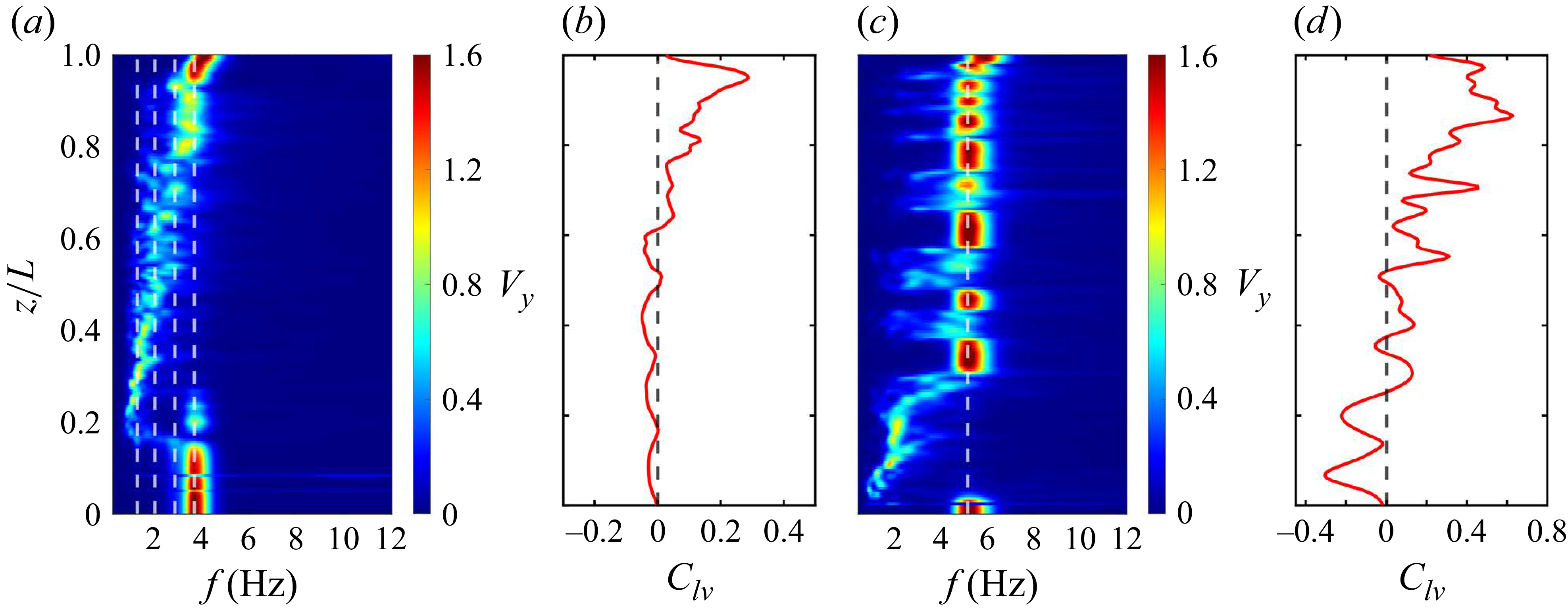
Furthermore, the PSD of the wake flow and the spanwise evolution of the energy transfer parameter
 $C_{lv}$
are shown in figure 20. For
 $Z_H=5.13$
, local single-frequency lock-in is again observed, similar to the cases at
 $U_{\infty }=0.20$
and
 $0.65$
ms−1, all of which belong to the multi-frequency response regime. For
 $Z_H=10.13$
, the characteristics are broadly similar to those observed at
 $U_{\infty }=0.38$
ms−1 as shown in figures 7 and 8, corresponding to the mono-frequency response regime. Taken together, the wake vortex characteristics across different initial geometric configurations closely parallel those observed under varying incoming velocities. This consistency confirms that the regime classification proposed in § 3.3 remains applicable for a range of initial geometries. In the following section, we further investigate how the three regimes are modulated by the initial geometric configuration.
 $(a,c)$
Temporal spectral analysis of the CF component of the wake velocity along the spanwise line, and
 $(b,d)$
spanwise evolution of the fluid–structure energy transfer parameter
 $C_{lv}$
, for
 $(a,b)$
 $Z_H=5.13$
and
 $(c,d)$
 $Z_H=10.13$
. The black dashed lines in
 $(a,c)$
denote the frequencies identified in figure 17.

Distribution of spanwise regimes as a function of the vertical height
 $Z_H$
. The vertical dashed line indicates the boundary between different modal groups, as shown in figure 17. The red dots and green triangles denote the locations of
 $F_c$
and
 $S_c$
, respectively.

4.2. Modulation of spanwise regimes by initial geometric configuration
In this section, we focus on how the initial geometric configuration influences the spatial distributions of these three spanwise regimes and the physical mechanism underlying these regimes. As shown in figure 21, the structural resonance regime generally coincides with different initial configurations under the same modal group, except when
 $Z_H\gt 10.13$
. Within each modal group (vertical dashed lines), the proportion of the flow-induced lock-in regime increases with
 $Z_H$
, as highlighted by the black arrows in figure 21. This indicates greater energy input from the flow and leads to larger maximum vibration amplitudes
 $(A_y^{rms}/D)_{max}$
(as shown in figure 17), consistent with trends observed under varying incoming velocities (figures 2 and 11). The value of the critical position
 $F_c$
and
 $S_c$
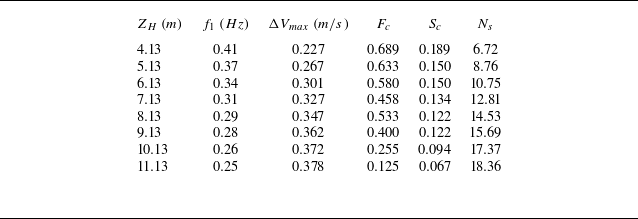
is summarised in table 2.
The main parameters of the CTRs under different vertical heights
 $Z_H$
.

Kim, Vandiver & Holler (Reference Leclercq and de Langre1986) and Vandiver (Reference Vandiver, Marcollo, Swithenbank and Jhingran1993) have identified two key parameters governing the occurrence of lock-in in long flexible cylinders subjected to ocean currents: the number of potentially excited modes,
 $N_s$
, and the shear fraction,
 $\beta$
, defined as
 \begin{equation} N_s=\frac {\Delta V}{f_1DV_r}, \quad\beta =\frac {\Delta V}{V_{max}}, \end{equation}
where
 $\Delta V$
denotes the velocity difference of the ocean current between two positions along the flexible cylinder,
 $f_1$
is the first natural frequency of the structure,
 $V_r$
represents the reduced velocity and
 $V_{max}$
is the maximum velocity experienced by the structure.
In general, the number of potentially excited modes
 $N_s$
can serve as a criterion for identifying the presence of partitioned lock-in: when
 $N_s$
approaches zero, the long flexible cylinder is effectively exposed to a uniform current. For
 $N_s\lt 1$
, the structure is highly prone to global single-frequency lock-in, whereas for
 $N_s\gt 100$
, lock-in does not occur. At intermediate values of
 $N_s$
, lock-in is confined to localised portions of the cylinder, with multiple modes invariably contributing to the response (Vandiver Reference Vandiver, Marcollo, Swithenbank and Jhingran1993). According to (4.1), the values of
 $N_s$
for different initial geometric configurations are summarised in table 2, with
 $V_r$
fixed at
 $5.9$
following Vandiver’s recommendation. The results show that
 $N_s$
falls within the range
 $6.72{-}18.36$
, indicating the occurrence of local lock-in accompanied by multi-modal responses, consistent with the earlier observations.
The shear fraction,
 $\beta$
, can serve as a criterion for identifying lock-in regions. Based on the normal-velocity component acting on the CTRs, (4.1) may be reformulated as
 $\beta =\Delta U_n/U_n^{\textit{max}}$
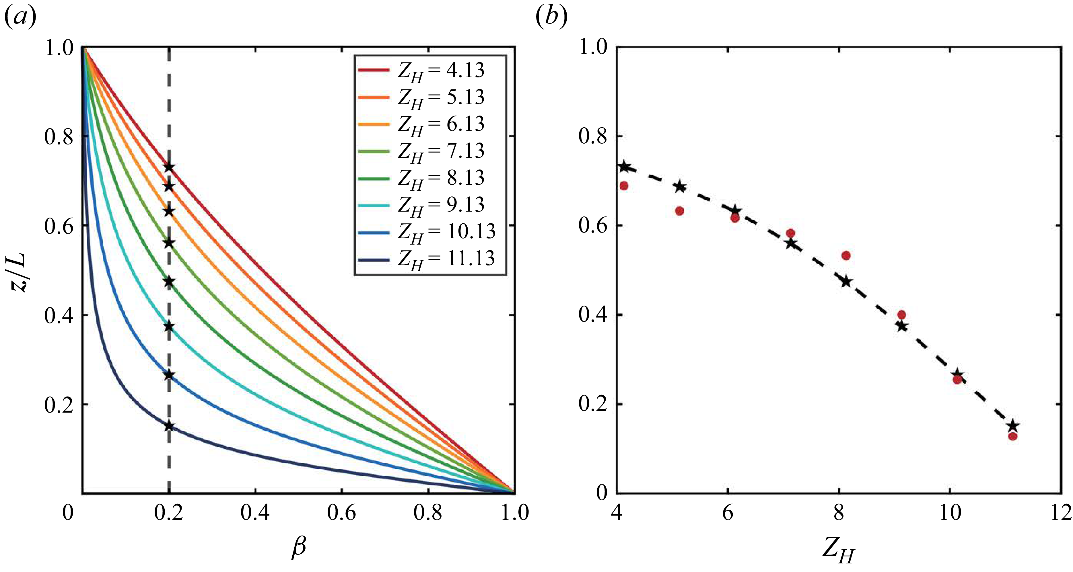
. Figure 22
 $(a)$
shows the spanwise distribution of
 $\beta$
for different
 $Z_H$
, indicating that
 $\beta$
decreases at a given spanwise location
 $z/L$
with increasing
 $Z_H$
. As shown in figure 22
 $(b)$
, we find that the position corresponding to
 $\beta =0.2$
coincides precisely with the boundary between the flow-induced lock-in and non-lock-in regimes identified in the numerical results for the CTRs under uniform incoming flow. The red solid symbols denote the numerical data extracted from figure 21, while the black pentagram symbols mark the theoretical positions where
 $\beta =0.2$
, obtained from the intersections of the vertical dashed lines with the velocity profiles in figure 22
 $(a)$
. This close agreement demonstrates that the onset of the flow-induced lock-in regime is affected by the relative velocity difference. Similarly, Vandiver (Reference Vandiver, Marcollo, Swithenbank and Jhingran1993) reported that, for flexible risers in linear shear currents, lock-in occurs within a shear fraction of approximately
 $20\,\,\%$
. Using data from the Norwegian Deepwater Programme experiments, Modarres-Sadeghi et al. (Reference Moe, Teigen, Simantiras, Willis and Lie2010) observed that this range could extend to more than
 $40\,\,\%$
under linear shear. For short-driven cylinders, Stansby (Reference Techet, Hover and Triantafyllow1976) suggested a threshold of approximately
 $25\,\,\%$
, whereas Griffin (Reference Griffin1985) proposed a broader value of approximately
 $30\,\%$
, consistent with the numerical results of Bourguet et al. (Reference Bourguet, Karniadakis and Triantafyllou2011a
) for flexible cylinders in linear shear.
 $(a)$
The normalised normal velocity normalised by the maximum of the normal velocity
 $\beta = \Delta U_n/U_n^{max}$
under different vertical heights
 $Z_H$
. The vertical dashed line represents the position of
 $20\,\%$
.
 $(b)$
Comparison of theoretical and numerical results under different vertical heights
 $Z_H$
fixed
 $U_{\infty }=0.38$
ms−1. Dashed line show theoretical results from
 $(a)$
, and symbols show numerical data from figure 21.

However, the underlying physical mechanisms driving these spanwise behaviours remain not fully understood and are largely described in qualitative terms. Bourguet et al. (Reference Bourguet, Karniadakis and Triantafyllou2011a
,
Reference Bourguet, Modarres-Sadeghi, Karniadakis and Triantafylloub
) identified two primary regions for vertical flexible cylinders in both linear and exponential shear: a lock-in region confined to high-velocity zones and a non-lock-in region in other areas. More recently, Zhu et al. (Reference Zhu, Zhang, Zhao, Xie, Tang and Zhou2023) categorised the axial response of the catenary flexible riser under shear flow into four coupling patterns based on vibration shape and frequency: strong coupling
 $^+$
, strong coupling, weak coupling and weak coupling
 $^-$
. In the following section, we examine in detail the physical processes underlying the observed spanwise regimes.
4.3. Physical mechanisms responsible for different spanwise regimes
As discussed above, the structural resonance regime is closely associated with the vibration mode number, and the flow-induced lock-in regime depends strongly on the relative velocity difference, which is jointly influenced by the incoming velocity and the initial configuration of the CTRs. In this subsection, we try to establish a reasonable model to understand these spanwise regimes.
First, the mechanism underlying the structural resonance regime is examined. The standing-wave length,
 $\lambda _s$
, is defined from the spanwise distribution of the phase difference of the dominant frequency. For instance, the dashed region where the phase difference remains constant corresponds to the standing-wave length near the bottom at
 $U_{\infty }=0.38$
ms−1 and
 $Z_H=7.13$
, and is illustrated in figure 23
 $(a)$
. The normalised critical positions
 $S_c/\lambda _s$
for various incoming velocities and initial configurations are presented in figures 23
 $(b)$
and 23
 $(c)$
, respectively. It is observed that the value of
 $S_c/\lambda _s$
is basically a constant of 1, except for cases with
 $Z_H\gt 10.13$
, where the strong curvature of the CTRs enhances flow–curvature interactions and induces a vertical velocity component not captured by strip theory (Assi et al. Reference Assi, Srinil, Freire and Korkischko2014), thereby leading to larger discrepancies. This consistency indicates that the the structural resonance regime is governed by the standing wave formed at the lower end of the structure. In this region, the normal component of the incoming flow is negligible, contributing minimally to excitation. Conversely, the fluid now exerts a damping effect, yielding
 $C_{lv}\lt 0$
, indicating energy transfer from the structure back to the fluid, as shown in figure 10. As vibrations generated near the upper section propagate downward as travelling waves, they reach the lower end and transition into standing waves, exciting the bottom region. The phase difference
 $\varPhi _{xy}$
exhibits a similar behaviour, as shown in figure 9. In this regime, the anti-node of the CF displacement corresponds to a node of the IL displacement, and the IL structural mode typically has twice the modal number of the CF mode (Bourguet et al. Reference Bourguet, Karniadakis and Triantafyllou2011a
). This process synchronises local vortex shedding with the structural motion rather than the local Strouhal frequency, leading to persistent overlap between the standing-wave zone and the structural resonance regime.
 $(a)$
The spanwise evolution of the phase angle of the dominant vibration frequency at
 $U_{\infty }=0.38$
ms−1 and
 $Z_H=7.13$
. Normalised critical position
 $S_c/\lambda _s$
vs incoming velocity
 $U_{\infty }$
and vertical height
 $Z_H$
in
 $(b)$
and
 $(c)$
, respectively.
 $(d)$
The critical position
 $S_c$
as a function of the mode number
 $n$
. The dashed line in
 $(d)$
represents the fitted scaling relation
 $S_c \sim n^{-1.0}$
.

Furthermore, when the structural response exhibits the
 $n$
th vibration mode, the standing-wave region near the bottom is expected to occupy approximately
 $1/n$
of the total length (Vandiver Reference Vandiver, Marcollo, Swithenbank and Jhingran1993; Facchinetti, de Langre & Biolley Reference Facchinetti, de Langre and Biolley2004; Williamson & Govardhan Reference Xia, Ren, Guo, Liu, Lin and Wang2004), as expressed
 \begin{equation} \lambda _s=\frac {1}{n}. \end{equation}
As shown in figure 23
 $(d)$
, a fitted power law between the critical position
 $S_c$
and the mode number, i.e.
 $S_c \sim n^{-1.0}$
, further confirms that the structural resonance regime is controlled by the standing wave formed at the lower end of the CTRs.
The mechanism underlying the flow-induced lock-in regime is examined further. When the structure experiences spanwise variations in the normal velocity (as shown in figure 16
 $(b)$
), the local Strouhal shedding frequency correspondingly varies along the span. Hence, the shear fraction
 $\beta$
quantifies the relative difference in the Strouhal vortex-shedding frequency. For a tensioned beam, the lock-in regions corresponding to different natural frequencies are mutually exclusive (Vandiver Reference Vandiver, Marcollo, Swithenbank and Jhingran1993). This implies that when the high normal velocity near the upper part drives the structure into lock-in with its
 $n$
th natural frequency, the remaining natural frequencies act as detuning factors that impede synchronisation. The spanwise variation of the normal velocity thus introduces this detuning effect. Consequently, once locked into the
 $n$
th mode, the structure exhibits perturbation resistance until the local Strouhal vortex-shedding frequency – determined by the normal velocity – approaches the
 $(n-1)$
th natural frequency. At this critical condition, the lock-in state breaks down, and the corresponding normal velocity can be expressed as
Comparison of theoretical and numerical results under
 $(a)$
different incoming velocities
 $U_{\infty }$
ms−1 and
 $(b)$
different vertical heights
 $Z_H$
. The red shaded area represents the range of theoretical results
 $\lambda _d$
under different Strouhal number from 0.20 to 0.22, and the black symbols show numerical data
 $F_c$
. The grey shaded area represents the multi-frequency response region.

 \begin{equation} U_n(z) = \frac {f_{n-1}D}{St}, \end{equation}
where
 $f_{n-1}$
is the
 $(n-1)$
th natural frequency. Applying the normal velocity
 $U_n(z)=U_{\infty }\cos (\theta )$
and (2.11), the corresponding axial position can be derived as
 \begin{equation} \frac {z}{L}=\frac {T_H}{W_eL\sqrt {\left(\dfrac{U_{\infty }St}{f_{n-1}D}\right)^2-1}}. \end{equation}
Following the work by Xia et al. (Reference Zheng and Wang2025), the horizontal static tension
 $T_H=(L^2-Z_H^2)/2Z_H$
. Finally, we get the critical detuning length
 $\lambda _d$
, expressed as
 \begin{equation} \lambda _d=\frac {z}{L}=\frac {L^2-Z_H^2}{2Z_HL\sqrt {\left(\dfrac{U_{\infty }St}{f_{n-1}D}\right)^2-1}}. \end{equation}
Equation (4.5) reveals that the critical position marking the onset of the transition from the flow-induced lock-in regime to the non-lock-in regime depends on the incoming velocity
 $U_{\infty }$
, the vertical height
 $Z_H$
and the natural frequency
 $f_{n-1}$
. This dependence implies that the modal order influences the relative extent of the flow-induced lock-in region, consistent with our earlier observation of jumps in the critical position
 $F_c$
between different modal groups. Furthermore, when the modal group and initial configuration are fixed (i.e.
 $f_{n-1}$
and
 $Z_H$
remain constant), an increase in
 $U_{\infty }$
leads to a decrease in
 $F_c$
, as shown in figure 11. Conversely, when the modal group and incoming velocity are held constant, increasing the vertical height
 $Z_H$
also results in a reduction of
 $F_c$
, consistent with the trend observed in figure 21.
Figure 24 shows the comparison of the analytical solution from (4.5) and numerical data under different incoming velocities
 $U_{\infty }$
and different vertical heights
 $Z_H$
. The Strouhal number
 $St$
, which also influences the transition, typically ranges between 0.20 and 0.22 within the present Reynolds number range (
 $1660 \leqslant Re \leqslant 11067$
) (Williamson & Govardhan Reference Xia, Ren, Guo, Liu, Lin and Wang2004). Accordingly, a theoretical band corresponding to this
 $St$
interval is plotted. At lower flow velocities, the numerical results align well with the upper bound of this theoretical band, whereas at higher velocities, they tend toward the lower bound, consistent with the gradual increase of
 $St$
with Reynolds number (Williamson & Govardhan Reference Xia, Ren, Guo, Liu, Lin and Wang2004). In the modal-transition region, deviations arise due to the coexistence and interaction of multiple frequency components, partially diminishing the exclusivity of frequency-locking zones associated with distinct natural frequencies. Moreover, the high normal-velocity-induced lock-in enhances structural vibrations through fluid to structure energy transfer, yielding
 $C_{lv}\gt 0$
, as shown in figure 10. Overall, the close agreement between the theoretical predictions and numerical results across different
 $U_{\infty }$
and
 $Z_H$
confirms the robustness of (4.5).
In conclusion, this study elucidates the underlying mechanisms governing the spanwise response regimes of CTRs. These findings provide new physical insight into the dynamics of curved flexible structures and offer guidance for the prediction, suppression and control of VIVs.
5. Summary
We have performed a series of numerical simulations of the VIV of the CTRs to investigate the spanwise response characteristics along the span of the CTRs under the uniform flow based on the strip-theory-based DVM. The simulations across a range of incoming velocities from
 $U_{\infty }=0.12$
to
 $U_{\infty }=0.80$
ms−1 (
 $1660\leqslant Re\leqslant 11\,067$
) and a range of different configurations from
 $Z_h=4.13$
to
 $Z_h=11.13$
. Adopting the tensioned Euler–Bernoulli beam with the IP, we quantified the structural response and the wake patters of the CTRs.
First, a modal-group switching phenomenon was identified through the analysis of the maximum normalised r.m.s. displacement
 $(A_y^{rms}/D)_{max}$
and dominant frequency
 $f_y$
. Within a given modal group,
 $(A_y^{rms}/D)_{max}$
increased monotonically with
 $U_{\infty }$
, while
 $f_y$
remains locked onto the natural frequency of the corresponding mode number
 $n$
. Once the flow velocity exceeded a threshold, the response transitioned to a new modal group, characterised by a reduction in
 $(A_y^{rms}/D)_{max}$
and a shift of both
 $f_y$
and mode number
 $n$
to the next natural frequency. Second, the results reveal a clear connection between mono-frequency and multi-frequency responses governed by modal-group switching. Within each modal group, the CTRs exhibited a mono-frequency response, where a single dominant frequency remained locked along the span and the phase angle varied monotonically, forming a travelling wave from the high normal-velocity top toward the low normal-velocity bottom. In the modal-transition region, the response became multi-frequency, comprising a sequence of temporally drifting instantaneous mono-frequency events. The corresponding phase angles displayed non-monotonic spanwise variations, leading to travelling-wave reflections in the spatio-temporal patterns. Despite these transitions, a mixed standing–travelling-wave pattern consistently emerged across all flow velocities and geometric configurations.
Further, three distinct spanwise regimes are identified from the FSI response, which are flow-induced lock-in regime (F-L regime), non-lock-in regime (N-L regime), and structure resonance regime (S-R regime). In the F-L regime, the vibration frequency locks onto the vortex-shedding frequency, with
 $C_{lv}\gt 0$
and predominantly CC trajectories, indicating that the normal-velocity component excites the vibration and transfers energy from the flow to the structure. In the N-L regime, the vortex-shedding frequency follows the local Strouhal-based frequency rather than the vibration frequency, accompanied by cellular wake patterns, with
 $C_{lv}\lt 0$
and predominantly C trajectories almost everywhere. In the S-R regime, the vibration frequency again locks onto the vortex-shedding frequency, but with
 $C_{lv}\lt 0$
and an approximately constant
 $\varPhi _{xy}$
, showing that energy is transferred back from the structure to the flow. In this regime, standing-wave behaviour dominates and the vibration is damped. The spatial extent of these regimes exhibits distinct scaling behaviours. The proportion of the S-R regime remains nearly independent of the incoming velocity but correlates strongly with the vibration mode number: for a given mode, the relative extent of the S-R regime is constant, while it decreases progressively with increasing mode number. In contrast, the F–L regime expands with increasing flow velocity within the same modal group, and its upper boundary coincides approximately with the shear fraction location at
 $\beta \approx 0.2$
. Moreover, the spanwise regimes correlate closely with the wake topology. The F–L regime is primarily associated with the ‘2P’ shedding mode, occasionally transitioning to a ‘2S’ pattern; the N–L regime features irregular or intermittent shedding, including a ‘2S-like’ mode; while the S-R regime is dominated by the ‘P+S’ pattern.
Building on these observations, we further elucidate the physical mechanisms underlying the different spanwise regimes. Two intrinsic length scales are found to govern the CTR spanwise partitioning response: the lower-span standing-wave length
 $\lambda _s$
and the critical detuning length
 $\lambda _d$
. The critical position
 $S_c$
, marking the onset of transition from S-R to N-L regime, is controlled by
 $\lambda _s=1/n$
, scaling inversely with mode number
 $S_c \sim n^{-1.0}$
. In contrast, the critical position
 $F_c$
, denoting the transition from F-L to N-L regime, is determined by
 $\lambda _d=(L^2-Z_H^2)/(2Z_HL\sqrt {({U_{\infty }St}/{f_{n-1}D})^2-1})$
. The theoretical predictions are shown to be in perfect agreement with the numerical results for all cases studied.
Overall, these findings demonstrate the spanwise partitioning of VIV responses in CTRs under uniform flow and provide a dual-scale framework for understanding their underlying mechanisms. The results carry significant engineering implications, enabling the prediction and mitigation of VIV by targeting sensitive axial regions. For instance, modifying the initial configuration to reduce the axial extent of the F–L regime can lower energy input, suppress vibration amplitudes and extend service life. The study also offers valuable guidance for developing VIV suppression strategies and simplified low-order models for fatigue assessment and offshore structure design.
Acknowledgements
The authors acknowledge the support provided by the National Natural Science Foundation of China.
Funding
This work was supported by the National Natural Science Foundation of China (grant nos. U2441218 and 12502281).
Declaration of interests
The authors report no conflict of interest.
Appendix. Validation cases for the algorithm
The present algorithm is validated against three experimental datasets. The first were performed in the towing tank at MARINTEK in Trondheim, Norway by Lie et al. (Reference Lin, Sun, Liu, Zhu, Wang, Triantafyllou and Fan2001), where a steel catenary riser was mounted on a vertical frame and exposed to a uniform current. The main parameters are summarised in table 1. Figure 25
 $(a{-}c)$
compares the dominant frequency, vibration mode number and the maximum of the normalised r.m.s. CF displacement
 $(A_y^{rms}/D)_{max}$
with the experimental data and the semi-empirical model VIVANA (evaluated with two Strouhal numbers, one using the default curve and the other fixed at
 $0.24$
), respectively. Both frequency and mode number exhibit stepwise growth with incoming velocity, in excellent agreement with the experiments and consistent with VIVANA, whereas
 $(A_y^{rms}/D)_{max}$
shows improved agreement with the experiments.
Comparison of
 $(a)$
the dominant frequency,
 $(b)$
vibration mode number and
 $(c)$
the normalised maximum r.m.s. CF displacement
 $(A_y^{rms}/D)_{max}$
of the structure with the experimental and numerical results of Lie et al. (Reference Lin, Sun, Liu, Zhu, Wang, Triantafyllou and Fan2001).
 $(d)$
Spanwise distribution of
 $A_y^{rms}/D$
at
 $U_{\infty }=0.26$
ms−1, compared with experimental (Moe et al. Reference Morooka and Tsukada2004) and numerical (Liu et al. Reference Liu, Li, Qiu, Leng, Li and Li2024) data.

The second case is based on the STRIDE experiments by Moe et al. (Reference Morooka and Tsukada2004), also performed at MARINTEK, which investigated the VIV response of CTRs with varying inclined angles. The key parameters are listed in table 1. For three representative incoming velocities, comparisons of the dominant frequency
 $f_y$
, vibration mode number
 $n$
and normalised maximum amplitude
 $A_y^{max}/D$
demonstrate excellent agreement between the present algorithm and the experimental results, as shown in table 3. Importantly, the accuracy of the present predictions surpasses that of the VICoMo model proposed by Moe et al. (Reference Morooka and Tsukada2004), with maximum discrepancies below
 $5\,\%$
. Furthermore, figure 25
 $(d)$
shows the spanwise distribution of
 $A_y^{rms}/D$
at
 $U_{\infty }=0.26$
ms−1, where the present algorithm achieves near-perfect agreement with the experiments and substantially outperforms the wake-oscillator-based model of Liu et al. (Reference Liu, Li, Qiu, Leng, Li and Li2024). Further details about the wake, computational efficiency and extended discussions are available in our earlier work (Xia et al. Reference Zheng and Wang2025).
Comparison of the normalised maximum amplitude
 $A_y^{\textit{max}}/D$
, the dominant frequency
 $f_y$
, and the mode number
 $n$
of the CTRs at three representative incoming velocities with the experimental results reported by Moe et al. (Reference Morooka and Tsukada2004).

Comparison with the experimental results of Zhu et al. (Reference Zhu, Lin and Yao2016): (a) initial geometric configuration;
 $(b)$
velocity profile
 $U_z$
(ms−1);
 $(c)$
normal-velocity component
 $U_n$
(ms−1); and
 $(d)$
the axial tension
 $T_s$
(N) along the CTR span.

The third case is based on the recirculating water-channel experiments of Zhu, Lin & Yao (Reference Zhu, Lin and Yao2016), which investigated the VIV response of CTRs under shear flow. The key parameters are also listed in table 1. As shown in figures 26(a) and 26(b), the initial configuration of the CTR and the shear-flow velocity profile are compared with the experimental measurements, showing good agreement and ensuring consistent simulation initial conditions. Subsequently, the IP is applied to determine the normal velocity
 $U_n$
(ms−1) and the axial tension
 $T_s$
(N) along the span, as shown in figures 26(c) and 26(d), respectively. The r.m.s. values of the IL and CF displacements are then compared with the experimental results, as shown in figure 27. The distribution of
 $A_{Xrms}/D$
exhibits a second-order modal response with noticeable non-periodicity, with the maximum occurring at
 $z/L = 0.74$
, which is slightly lower than the experimental value. In the middle region of the CTR, the numerical results are slightly higher and smoother than the experimental measurements, but the average difference remains below
 $5\,\%$
. Overall, the numerical results capture the main response characteristics well. Similarly,
 $A_{Yrms}/D$
also shows features of a second-order modal response with non-periodicity. Its maximum occurs at
 $z/L = 0.22$
, where the numerical prediction is again slightly lower than the experimental measurement, with only a small discrepancy. Overall, good agreement is observed between the numerical and experimental results.
Comparison of the r.m.s. values of the IL and CF displacements with the experimental results: (a) IL displacement; (b) CF displacement.

Furthermore, the motion trajectories of the CTR at several representative positions are compared with the experimental results, as shown in figure 28. The vertical locations of the selected rings are shown on the left, and their trajectories in the X–Y plane are shown on the right, with identical axis scales. For
 $z/H\lt 0.2$
, the trajectories evolve into a line-shaped pattern due to the combined effects of logarithmic shear flow and axial tension, which significantly reduce the streamwise displacement (Zhu et al. Reference Zhu, Lin and Yao2016). For
 $z/H\gt 0.6$
, the trajectories decrease proportionally in size toward the surface, mainly due to increasing axial tension, while the normal velocity varies little in the upper region. Near both ends of the CTR, the trajectories gradually distort into half-moon or C-shaped patterns, consistent with experimental observations. The numerical results reproduce these features accurately.
Comparison of the response trajectories of motion for the CTRs with the experimental results.

The instantaneous wake patterns at different spanwise locations of the CTR under the G15 inflow condition are compared with experimental results in figure 29. In the simulations, red and blue dots denote positive and negative vorticity, respectively, with schematic arrows indicating the vortex rotation direction. Different vortex-shedding modes, including 2P and P+S, are observed along the span, and the wake patterns predicted by the present numerical method show good agreement with the experiments. This demonstrates that the strip-theory-based approach can accurately capture the wake dynamics of catenary risers, and that weak three-dimensional effects do not significantly affect its applicability, consistent with Zhu et al. (Reference Zhu, Lin and Yao2019a ).
Comparison of locally instantaneous wake patterns at representative locations along the CTR with experimental results.

Comparison of the global vortex-shedding patterns at representative locations along the CTRs with experimental results. The colour bar in (b) represents the CF vibration amplitude normalised by the cylinder diameter.

The global wake pattern of the CTR, composed of seventeen representative instantaneous flow fields, is compared with the experimental results in figure 30. The colour bar in figure 30(b) represents the CF vibration amplitude normalised by the cylinder diameter. The numerical results show excellent agreement with the experiments, further confirming the validity and applicability of the proposed method for CTR structures. The complex wake structures also reveal strong spatial variation and zonal behaviour along the span, in line with previous studies (Seyed-Aghazadeh et al. Reference Seyed-Aghazadeh, Budz and Modarres-Sadeghi2021; Xia et al. Reference Zheng and Wang2025).
In summary, these validations confirm both the accuracy and efficiency of the proposed algorithm for simulating the VIV response of CTRs. By directly computing unsteady hydrodynamic forces without relying on empirical parameters, the method provides higher predictive capability than existing reduced-order models.