1 Introduction
Recent advances in the study of voting behavior and the study of legislatures have relied on ideal point estimation for measuring the preferences of political actors, and increasingly, these applications have involved very large data matrices. Large-scale problems include Poole and Rosenthal’s (Reference Poole and Rosenthal1997) DW-Nominate Common Space (DWCS) measure of the ideal points of members of House and Senate from the first to the current Congress, Shor and McCarty’s (Reference Shor and McCarty2011) measure of the ideal points of legislators for the 99 state legislatures ranging from 1993 to 2016, and Tausanovitch and Warshaw’s (Reference Tausanovitch and Warshaw2013) estimates of the ideal points of a few hundred thousand survey respondents from 2000 to 2011.
Applications of ideal point estimation have typically relied on Poole and Rosenthal’s (Reference Poole and Rosenthal1991, Reference Poole and Rosenthal1997) zigzag method (as implemented in wnominate), Jackman (Reference Jackman2001) and Martin and Quinn’s (Reference Martin and Quinn2002) Bayesian approach using data augmentation (as implemented in ideal), and Imai, Lo, and Olmsted’s (Reference Imai, Lo and Olmsted2016) EM approach (as implemented in emIRT). Large-scale ideal point estimation has, however, proved challenging for the widely available approaches, and studies involving large datasets have often applied specialized software. Poole and Rosenthal’s (Reference Poole and Rosenthal1997) DWCS estimates relied on a program that is not available for others to use and is specialized to chambers with overlapping membership. Shor and McCarty’s (Reference Shor and McCarty2011) estimates are based on linear mapping, and better estimates could potentially be arrived at using joint estimation. Tausanovitch and Warshaw’s (Reference Tausanovitch and Warshaw2013) estimates relied on a specialized Gibbs sampler implemented to run on graphics processing units.
The three widely available methods each suffer from some limitations. All three methods do not efficiently deal with sparse data matrices—data matrices where most of the entries are missing. Most large-scale ideal point estimation problems involve connecting many chambers (e.g., different sessions of Congress) using a small number of bridge voters or bridge votes, leading to very sparse data matrices. This means that in large-scale applications, existing methods will be slow and consume excessive memory. wnomimate and emIRT employ the parametric bootstrap for computing standard errors and therefore become many times slower when standard errors are needed. None of the three methods have fully adequate approaches for computing starting values, and in large-scale applications, the estimators will not converge properly in the absence of good starting values. emIRT can only estimate one-dimensional ideal points.
Even the two specialized methods share many of these limitations (beyond the fact that they are not readily available to other scholars).Footnote 1 The DWCS estimator efficiently deals with sparse data matrices, but not in a way that generalizes beyond the intended application. DWCS requires the parametric bootstrap to compute standard errors. The Gibbs sampler employed by Tausanovitch and Warshaw (Reference Tausanovitch and Warshaw2013) cannot efficiently handle sparse data matrices. Neither approach has solved the problem of computing starting values for large-scale problems.
In this paper, I focus on developing methods for estimating multidimensional ideal points in large-scale applications in a computationally efficient manner. The methods I develop solve large-scale problems quickly, are efficient in the presence of sparse data matrices, and can efficiently compute standard errors. In addition, I provide a computationally efficient approach for generating starting values for both dense and sparse data matrices. I develop these methods in an r package (ipe). The main algorithm optimizes a penalized maximum likelihood objective function using limited memory BFGS. Standard errors are calculated using the asymptotic Hessian.
I compare my method to three existing methods for ideal point estimation—wnominate, ideal, and emIRT. With good starting values, my method and the alternative methods produce very similar results, but vary substantially in the time they take to execute and the memory they consume. My approach is significantly faster than wnominate and ideal across a broad range of circumstances. emIRT achieves impressive performance across many applications, but my approach is more computationally efficient than emIRT when the data matrix is sparse and when standard errors are required. On many large-scale applications, emIRT will not converge properly due to the absence of appropriate starting values. For the largest applications I consider, alternative methods require excessive memory, while my method can solve each of these problems in less than a few hours on a laptop computer.
2 Model
Consider the
 $N\times T$
data matrix y with elements
 $y_{nt} $
, where n denotes individuals or voters and t denotes items or votes. Assume that
 $y_{nt} \in \{ 1,2\}, $
where
 $y_{nt} =2$
denotes a yea vote and
 $y_{nt} =1$
denotes a nay vote. Each individual is characterized by a (potentially multidimensional) ideal point
 $\alpha _{n} \in {\mathbb R}^{D} $
, where
 $D\ge 1$
and each item is characterized by a (potentially multidimensional) cutting plane, with
 $a_{t} \in {\mathbb R}$
and
 $b_{t} \in {\mathbb R}^{D} $
. Assume that we observe
 $y_{nt} =2$
with probability
 $\Phi (a_{t} +b_{t} '\alpha _{n} )$
and
 $y_{nt} =1$
with probability
 $1-\Phi (a_{t} +b_{t} '\alpha _{n} )$
, and assume that these probabilities are independent across n and t.
This model can be viewed as arising from a latent variable model. Specifically,
 $y_{nt}^*=a_{t} +b_{t} '\alpha _{n} +\varepsilon _{nt} $
, where
 $\varepsilon _{nt} $
are independent
 $N(0,1)$
errors and
 $y_{nt} =2\Leftrightarrow 1\{ y_{nt}^* \ge 0\} $
. The latent variable model itself can be viewed as arising from a random utility model. Suppose that the utility for voting for the proposal (
 $y_{nt} =2$
) is given by
 $u_{nt}^{p} =-(\alpha _{n} -p_{t} )'W(\alpha _{n} -p_{t} )+\varepsilon _{nt}^{p} $
and the utility of voting for the status quo (
 $y_{nt} =1$
) is given by
 $u_{nt}^{s} =-(\alpha _{n} -s_{t} )'W(\alpha _{n} -s_{t} )+\varepsilon _{nt}^{s} $
, where
 $p_t \in {\mathbb R}^{D}$
is a proposal location,
 $s_t \in {\mathbb R}^{D}$
is a status quo location, and W is a positive definite matrix. Assume that
 $\varepsilon _{nt}^{p} -\varepsilon _{nt}^{s} \sim N(0,\sigma _{t} )$
, where
 $\sigma _{1} $
is normalized to 1. A yea vote is observed when
 $u_{nt}^{p} \ge u_{nt}^{s} $
, or when
 $u_{nt}^{p} -u_{nt}^{s} =-p_{t} 'Wp_{t} +s_{t} 'Ws_{t} +2(p_{t} -s_{t} )'W\alpha _{n} +\varepsilon _{nt}^{p} -\varepsilon _{nt}^{s} \ge 0$
. The two models can be related by setting
 $y_{nt}^*=u_{nt}^{p} -u_{nt}^{s} $
,
 $a_{t} =\frac {-p_{t} 'Wp_{t} +s_{t} 'Ws_{t} }{\sigma _{t} } $
,
 $b_{t} =\frac {2(p_{t} -s_{t} )'W\alpha _{n} }{\sigma _{t} } $
, and
 $\varepsilon _{nt} =\frac {\varepsilon _{nt}^{p} -\varepsilon _{nt}^{s} }{\sigma _{t} } $
. The item response model can thus be viewed as a reduced form of the binary random utility model where
 $\alpha _{n} $
are the ideal points.
The model described here is most similar to Jackman (Reference Jackman2001) and is often called the two-parameter item response theory model (it differs from Jackman (Reference Jackman2001) only in the parameterization). Imai et al. (Reference Imai, Lo and Olmsted2016) consider multiple models, but the model described here is equivalent to their “standard ideal point model.” Poole and Rosenthal’s (Reference Poole and Rosenthal1991, Reference Poole and Rosenthal1997) model is similar, but employs Gaussian utilities and extreme value errors.Footnote 2 In addition, some of their models allow ideal points to evolve over time as a polynomial. Various papers in the literature use similar models with different deterministic utilities and different error term distributions. It has generally been found that such differences in the underlying model, as well as differences in the estimation approach, lead to similar results—see Figure 2 in Imai et al. (Reference Imai, Lo and Olmsted2016), for example.
3 Details of the Algorithm
3.1 Estimating the Parameters
The log-likelihood for the model is
 $$ \begin{align} l(\alpha ,a,b)=\sum _{n=1}^{N}\sum _{t=1}^{T}\left\{1\{ y_{nt} =2\} \log \Phi (a_{t} +b_{t} '\alpha _{n} )+1\{ y_{nt} =1\} \log [1-\Phi (a_{t} +b_{t} '\alpha _{n} )]\right\}. \end{align} $$
The penalized log-likelihood can be formed as
 $$ \begin{align} Q(\alpha ,a,b)=l(\alpha ,a,b)+\lambda _{\alpha } \sum _{n=1}^{N}\alpha _{n} '\alpha _{n} +\lambda _{\delta } \sum _{t=1}^{T}(a_{t} ,b_{t} )'(a_{t} ,b_{t} ) \end{align} $$
with penalty parameters
 $\lambda _{\alpha }>0$
and
 $\lambda _{\delta }>0$
.Footnote
3
My algorithm estimates
 $\alpha $
, a, and b by maximizing
 $Q(\alpha ,a,b)$
over
 $(\alpha ,a,b)$
. The penalty terms are included in the objective function, because the ideal points are only identified up to a linear transformation. The penalty terms are one way of preventing the objective function from having no strict local maxima. The optimization approach I apply would perform poorly if applied to a function with no strict local maxima, and the penalized objection function helps avoid these problems.Footnote
4
Because the likelihood involves a double sum and the penalty terms involve a single sum, the influence on the penalty becomes smaller and smaller as the sample size increases. Maximizing the penalized objective function is equivalent to maximizing a Bayesian posterior for this model, with normal mean-zero independent priors for all parameters. A penalized objective function is not the only way to deal with the nonidentification of the ideal points—Poole and Rosenthal (Reference Poole and Rosenthal1997), for example, used inequality constraints on the parameter space—but this approach allows me to apply efficient methods of numerical optimization.
My approach for maximizing
 $Q(\alpha ,a,b)$
is a variant of the Quasi-Newton method. Quasi-Newton methods are the default method for nonlinear optimization recommended by many optimization texts, but have been avoided by scholars working on the ideal point estimation problem, because they were believed to be too computationally costly. Poole and Rosenthal (Reference Poole and Rosenthal1991, Reference Poole and Rosenthal1997) developed an alternative approach for optimizing the ideal point likelihood to get around the presumed insurmountable computational cost of applying Quasi-Newton methods. Indeed, naive implementations of Quasi-Newton methods involve such insurmountable costs when applied to ideal point estimation. Below, I demonstrate how these methods can be applied efficiently.
At each iteration, the Quasi-Newton method requires calculating
 $Q(\alpha ,a,b)$
and
 ${\tfrac {\partial }{\partial (\alpha ,a,b)}} Q(\alpha ,a,b)$
. To analyze the computational cost of the algorithm, I employ “big O notation.” Here,
 $O(f(n))$
indicates that a given computation requires on the order of
 $f(n)$
operations, where f is a function, n is the size of the input to the algorithm, and an operation refers to a computation step (e.g., addition, multiplication, etc.). For example, if the algorithm requires
 $2n^2 -3n + 7$
operations, we would say that it requires
 $O(n^2)$
operations. The order of operations thus capture how quickly the computational cost grows as the size of the problem grows. It captures the fact that for large enough problems, the
 $-3n + 7$
will be negligible relative to
 $2n^2$
. By ignoring the
 $2$
in front of
 $n^2$
, it emphasizes the fact that an
 $an^2$
algorithm is likely to be much slower than a
 $bn$
algorithm, for most values of a and b.
Calculating
 $Q(\alpha ,a,b)$
involves
 $O(NT)$
operations. A naive approach for calculating the gradient,
 ${\tfrac {\partial }{\partial (\alpha ,a,b)}} Q(\alpha ,a,b)$
, would rely on a finite difference approximation. Given that the number of variables is
 $DN+(D+1)T$
, doing so would require
 $O(NT\max (N,T) )$
operations. The Quasi-Newton method using the standard BFGS approximation to the Hessian would require solving
 $B^{-1} g$
, where B is the BFGS approximation and g is the gradient. Applying the naive version of the BFGS approach would require
 $O(\max (N,T) ^{3} )$
operations per iteration overall.
This cost can be brought down in two ways. First,
 $B^{-1} g$
does not have to be solved at each iteration. Each iteration of the Quasi-Newton method involves a rank-one update to the matrix B (Dennis and Schnabel Reference Dennis and Schnabel1983). Instead of reforming
 $B^{-1} $
at each iteration, a Cholesky decomposition of
 $B^{-1} $
can be maintained. At each iteration, this requires applying a rank-one update of
 $B^{-1} $
and solving two triangular systems of equations. The overall cost is
 $O(\max (N,T) ^{2} )$
operations. The linear algebra cost can be brought down further by considering a limited memory BFGS update (Gill, Murray, and Wright Reference Gill, Murray and Wright1981). In this case, a factorization B is not retained. Instead, the iterates and gradients from the last m iterations are retained, where m is typically between 5 and 20. In this case, the cost of the linear algebra is
 $O(\max ( N,T) )$
operations. Beyond the decrease in computation time, limited memory BFGS reduces the memory requirements—while BFGS requires
 $O(\max (N,T) ^{2} )$
memory, limited memory BFGS requires
 $O(\max ( N,T) )$
memory.
Second, the derivatives of
 $Q(\alpha ,a,b)$
can be calculated as
 $$ \begin{align} {\tfrac{\partial }{\partial \alpha _{n} }} Q(\alpha ,a,b)&=\sum _{t=1}^{T}\Bigg\{1\{ y_{nt} =2\} \frac{\phi (a_{t} +b_{t} '\alpha _{n} )}{\Phi (a_{t} +b_{t} '\alpha _{n} )} b_{t} -1\{ y_{nt} =1\} \frac{\phi (a_{t} +b_{t} '\alpha _{n} )}{1-\Phi (a_{t} +b_{t} '\alpha _{n} )} b_{t} \Bigg\} +2\lambda _{\alpha } \alpha _{n}, \end{align} $$
 $$ \begin{align} {\tfrac{\partial }{\partial (a_{t} ,b_{t} )}} Q(\alpha ,a,b)&=\sum _{n=1}^{N}\Bigg\{1\{ y_{nt} =2\} \frac{\phi (a_{t} +b_{t} '\alpha _{n} )}{\Phi (a_{t} +b_{t} '\alpha _{n} )} (1,\alpha _{n} )\nonumber\\ &\qquad-1\{ y_{nt} =1\} \frac{\phi (a_{t} +b_{t} '\alpha _{n} )}{1-\Phi (a_{t} +b_{t} '\alpha _{n} )} (1,\alpha _{n} )\Bigg\} +2\lambda _{\delta } (a_{t} ,b_{t} ). \end{align} $$
This implies that the cost of calculating the gradient is
 $O(NT)$
operations. Combined, our total cost is
 $O(NT)$
operations per iteration of the limited memory BFGS algorithm, which is much smaller than the cost of the naive approach, which would require
 $O(\max ( N,T)^3 )$
operations per iteration and would require
 $O(\max ( N,T)^2 )$
memory.
The two aspects of my approach—reducing the cost of linear algebra using limited memory BFGS and reducing the cost of computing the gradient—are not unknown to the field of numerical optimization—in fact, these are standard recommendations. Limited memory BFGS is the default approach for large-scale optimization recommended in many textbooks (Gill et al. Reference Gill, Murray and Wright1981; Nocedal and Wright Reference Nocedal and Wright2006) and is implemented in high-quality optimization software (Gill, Murray, and Wright Reference Gill, Murray and Wright2002; Byrd, Nocedal, and Waltz Reference Byrd, Nocedal, Waltz, Di Pillo and Roma2006). A well-known result in the optimization literature is that the gradient of a function can be calculated in no more than five times the cost of evaluating the function itself (Griewank and Walther Reference Griewank and Walther2008). Reducing the cost of linear algebra using limited memory BFGS simply requires using good optimization routines, as opposed to the widely applied dfpmin (from Numerical Recipes) and optim (implemented in r). Reducing the cost of computing the gradient requires differentiating the gradient by hand (as is done in Equation (3)) and supplying it to the optimization software, rather than relying on the finite difference approximation to the gradient. Finally, it is worth mentioning that the alternative methods I compare my method to also achieve a cost of
 $O(NT)$
operations per iteration. This subsection demonstrates that my method is competitive with the other methods and demonstrates why it is competitive. Sections 3.2 and 3.3 below identify instances where my method is likely to be superior to alternative methods. Section 5 further below accounts for the number of iterations and the cost per iteration for the various methods to identify when my method performs better than alternative approaches.
3.2 Estimating the Variance–Covariance Matrix
The second derivatives of the objective function can be calculated as follows:
 $$ \begin{align} &\tfrac{\partial ^{2} }{\partial \alpha _{n} \partial \alpha _{n} '} Q(\alpha ,a,b)\nonumber\\ &= \sum _{t=1}^{T}\left\{\begin{array}{l} {1\{ y_{nt} =2\} \frac{\Phi (a_{t} +b_{t} '\alpha _{n} )\phi '(a_{t} +b_{t} '\alpha _{n} ) -\phi (a_{t} +b_{t} '\alpha _{n} )^{2} }{\Phi (a_{t} +b_{t} '\alpha _{n} )^{2} } b_{t} b_{t} '} \\ {-1\{ y_{nt} =1\} \frac{(1-\Phi (a_{t} +b_{t} '\alpha _{n} ))\phi '(a_{t} +b_{t} '\alpha _{n} )+\phi (a_{t} +b_{t} '\alpha _{n} )^{2} }{(1-\Phi (a_{t} +b_{t} '\alpha _{n} ))^{2} } b_{t} b_{t} '} \end{array}\right\} +2\lambda _{\alpha } I, \end{align} $$
 $$ \begin{align} \tfrac{\partial ^{2} }{\partial \alpha _{n} \partial \alpha _{m} '} Q(\alpha ,a,b)=0, \end{align} $$
 $$ \begin{align*} \tfrac{\partial ^{2} }{\partial (a_{t} ,b_{t} )\partial (a_{t} ,b_{t} )'} Q(\alpha ,a,b) \notag \end{align*} $$
 $$ \begin{align} =\sum _{n=1}^{N}\left\{\begin{array}{l} {1\{ y_{nt} =2\} \frac{\Phi (a_{t} +b_{t} '\alpha _{n} )\phi '(a_{t} +b_{t} '\alpha _{n} )-\phi (a_{t} +b_{t} '\alpha _{n} )^{2} }{\Phi (a_{t} +b_{t} '\alpha _{n} )^{2} } (1,\alpha _{n} )(1,\alpha _{n} )'} \\ {-1\{ y_{nt} =1\} \frac{(1-\Phi (a_{t} +b_{t} '\alpha _{n} ))\phi '(a_{t} +b_{t} '\alpha _{n} )+\phi (a_{t} +b_{t} '\alpha _{n} )^{2} }{(1-\Phi (a_{t} +b_{t} '\alpha _{n} ))^{2} } (1,\alpha _{n} )(1,\alpha _{n} )'} \end{array}\right\} +2\lambda _{\delta } I, \end{align} $$
 $$ \begin{align} \tfrac{\partial ^{2} }{\partial (a_{t} ,b_{t} )\partial (a_{s} ,b_{s} )'} Q(\alpha ,a,b)=0, \end{align} $$
 $$ \begin{align} \tfrac{\partial ^{2} }{\partial \alpha _{n} \partial a_{t} } Q(\alpha ,a,b) =\left\{\begin{array}{l} {1\{ y_{nt} =2\} \frac{\Phi (a_{t} +b_{t} '\alpha _{n} )\phi '(a_{t} +b_{t} '\alpha _{n} )-\phi (a_{t} +b_{t} '\alpha _{n} )^{2} }{\Phi (a_{t} +b_{t} '\alpha _{n} )^{2} } b_{t} } \\ {-1\{ y_{nt} =1\} \frac{(1-\Phi (a_{t} +b_{t} '\alpha _{n} ))\phi '(a_{t} +b_{t} '\alpha _{n} )-\phi (a_{t} +b_{t} '\alpha _{n} )^{2} }{(1-\Phi (a_{t} +b_{t} '\alpha _{n} ))^{2} } b_{t} } \end{array}\right\}, \end{align} $$
 $$ \begin{align} \tfrac{\partial ^{2} }{\partial \alpha _{n} \partial b_{t} '} Q(\alpha ,a,b) =\left\{\begin{array}{l} {1\{ y_{nt} =2\} \frac{\Phi (a_{t} +b_{t} '\alpha _{n} )\phi '(a_{t} +b_{t} '\alpha _{n} )-\phi (a_{t} +b_{t} '\alpha _{n} )^{2} }{\Phi (a_{t} +b_{t} '\alpha _{n} )^{2} } b_{t} \alpha _{n} '} \\ {-1\{ y_{nt} =1\} \frac{(1-\Phi (a_{t} +b_{t} '\alpha _{n} ))\phi '(a_{t} +b_{t} '\alpha _{n} )+\phi (a_{t} +b_{t} '\alpha _{n} )^{2} }{(1-\Phi (a_{t} +b_{t} '\alpha _{n} ))^{2} } b_{t} \alpha _{n} '} \\ {+1\{ y_{nt} =2\} \frac{\phi (a_{t} +b_{t} '\alpha _{n} )}{\Phi (a_{t} +b_{t} '\alpha _{n} )} -1\{ y_{nt} =1\} \frac{\phi (a_{t} +b_{t} '\alpha _{n} )}{1-\Phi (a_{t} +b_{t} '\alpha _{n} )} } \end{array}\right\}. \end{align} $$
The structure of the Hessian matrix is that there are blocks along the diagonal, which are sums over N and T, and there is a lower left and upper right block which does not involve a sum. The Hessian can be represented as
 $$ \begin{align} H=\left[\begin{array}{cc} {H_{11} } & {H_{12} } \\ {H_{21} } & {H_{22} } \end{array}\right], \end{align} $$
where
 $$ \begin{align} [H_{11} ]_{mn} ={\tfrac{\partial ^{2} }{\partial \alpha _{m} \partial \alpha _{n} '}} Q(\alpha ,a,b), \end{align} $$
 $$ \begin{align} [H_{12} ]_{nt} ={\tfrac{\partial ^{2} }{\partial \alpha _{n} \partial (a_{t} ,b_{t} )'}} Q(\alpha ,a,b), \end{align} $$
 $$ \begin{align} [H_{21} ]_{tn} ={\tfrac{\partial ^{2} }{\partial (a_{t} ,b_{t} )\partial \alpha _{n} '}} Q(\alpha ,a,b), \end{align} $$
 $$ \begin{align} [H_{22} ]_{ts} ={\tfrac{\partial ^{2} }{\partial (a_{t} ,b_{t} )\partial (a_{s} ,b_{s} )'}} Q(\alpha ,a,b). \end{align} $$
Standard approaches for calculating the standard errors would require calculating
 $H^{-1}$
. Since the dimension of the Hessian is
 $ND+T(D+1)$
, standard algorithms for inverting the Hessian would involve
 $O(\max (N,T)^3)$
operations and would require
 $O(\max (N,T)^2)$
memory. This standard approach is infeasible on larger problems. For example, for the largest problem I consider, the memory requirement for storing the Hessian would be 221 gigabytes. My approach develops an asymptotically equivalent expression for Hessian that can be inverted without this insurmountable computational cost. In online Appendix A.2, I demonstrate that
 $\tfrac {1}{T} H $
converges to a block diagonal matrix in large samples. Since the limit is block-diagonal, it can be inverted by inverting the blocks.Footnote
5
Calculating H requires
 $O(NT)$
operations and inverting it requires
 $O(\max ( N,T))$
operations. Hence, inferences on the parameters can be performed in
 $O(NT)$
operations and require
 $O(\max (N,T))$
memory.
3.3 Sparse Data Matrices
In many cases, some voters will not vote on all items. I represent such a situation using a zero in the data matrix, i.e.,
 $y_{nt} = 0$
. When y is sparse—that is, it contains many zero entries—the penalized log-likelihood can be written as
 $$ \begin{align} &l(\alpha ,a,b)\nonumber\\ &=\sum _{n=1}^{N}\sum _{t=1}^{T}\bigg\{1\{ y_{nt} =2\} \log \Phi (a_{t} +b_{t} '\alpha _{n} )+1\{ y_{nt} =1\} \log [1-\Phi (a_{t} +b_{t} '\alpha _{n} )]\nonumber\\&\qquad+1\{ y_{nt} =0\} \log (1)\bigg\}\nonumber\\ &=\sum _{n,t:y_{nt} \ne 0}\bigg\{1\{ y_{nt} =2\} \log \Phi (a_{t} +b_{t} '\alpha _{n} )+1\{ y_{nt} =1\} \log [1-\Phi (a_{t} +b_{t} '\alpha _{n} )]\bigg\}. \end{align} $$
Let S be the number of nonzero entries in y. Computing the penalized log-likelihood, computing the gradient, computing the Hessian, and inverting the approximate Hessian each require
 $O(S)$
operations. Doing so requires storing y in an appropriate data structure, such as a compressed row or a compressed column matrix (Golub and Van Loan Reference Golub and Van Loan1996). The various steps require
 $O(S)$
memory. Compare this to the cost for dense data matrices—
 $O(NT)$
operations and
 $O(NT)$
memory. In the largest applications, I have found that S will often be less than 1% of
 $NT$
, leading to substantial increases in computational efficiency.Footnote
6
3.4 Computing Starting Values
One algorithm for computing starting values is widely known in the ideal point estimation literature. wnominate and ideal both base their starting values on an eigenvalue decomposition of the double-centered agreement score matrix. Below, I demonstrate an equivalent way of computing these starting values with lower computational costs and less memory required. Consider the complete data matrix y. Let
 $\bar {y}_{n,.} $
denote the individual means, let
 $\bar {y}_{.,t} $
denote the item means, and let
 $\bar {y}_{.,.} $
denote the overall mean. The double-centered matrix is given by
 $\tilde {y}=y-\bar {y}_{n,.} 1_{T} '-1_{N} \bar {y}_{.,t} '+1_{N} 1_{T} '\bar {y}_{.,.} $
, where
 $1_i$
denotes a vector of length i with all elements equal to
 $1$
. Note that the row means and column means are given by
 $$ \begin{align} \bar{\tilde{y}}_{n,.} ={\tfrac{1}{T}} \sum _{t=1}^{T}(y_{nt} -\bar{y}_{n,.} -\bar{y}_{.,t} +\bar{y}_{.,.} ) =\bar{y}_{n,.} -\bar{y}_{n,.} -\bar{y}_{.,.} +\bar{y}_{.,.} =0, \end{align} $$
 $$ \begin{align} \bar{\tilde{y}}_{.,t} ={\tfrac{1}{N}} \sum _{n=1}^{N}(y_{nt} -\bar{y}_{n,.} -\bar{y}_{.,t} +\bar{y}_{.,.} ) =\bar{y}_{.,t} -\bar{y}_{.,.} -\bar{y}_{.,t} +\bar{y}_{.,.} =0. \end{align} $$
The row-wise and column-wise variance elements are given by
 $$ \begin{align} \Omega _{mn}^{r} ={\tfrac{1}{T-1}} \sum _{t=1}^{T}(\tilde{y}_{nt} -\bar{\tilde{y}}_{n,.} )(\tilde{y}_{mt} -\bar{\tilde{y}}_{m,.} ) ={\tfrac{1}{T-1}} \sum _{t=1}^{T}\tilde{y}_{nt} \tilde{y}_{mt}, \end{align} $$
 $$ \begin{align} \Omega _{st}^{c} ={\tfrac{1}{N-1}} \sum _{n=1}^{N}(\tilde{y}_{nt} -\bar{\tilde{y}}_{.,t} )(\tilde{y}_{nt} -\bar{\tilde{y}}_{.,s} ) ={\tfrac{1}{N-1}} \sum _{n=1}^{N}\tilde{y}_{nt} \tilde{y}_{ns}. \end{align} $$
The singular value decomposition (SVD) can be applied to
 $\tilde {y}$
and the eigenvalue decomposition can be applied to
 $\Omega ^{r} ={\tfrac {1}{T-1}} \tilde {y}\tilde {y}'$
and
 $\Omega ^{c} ={\tfrac {1}{N-1}} \tilde {y}'\tilde {y}$
to obtain
 $$ \begin{align} \tilde{y}=USV', \end{align} $$
 $$ \begin{align} \Omega ^{r} =U_{r} \Lambda _{r} U_{r} ', \end{align} $$
 $$ \begin{align} \Omega ^{c} =V_{c} \Lambda _{c} V_{c} ', \end{align} $$
where
 $U'U = I$
,
 $V'V = I$
,
 $U_r'U_r = I$
, and
 $V_c' V_c = I$
. Notice that
 $$ \begin{align} \Omega ^{r} ={\tfrac{1}{T-1}} \tilde{y}\tilde{y}'={\tfrac{1}{T-1}} USV'VSU'={\tfrac{1}{T-1}} USSU'=U{\tfrac{1}{T-1}} S^{2} U', \end{align} $$
 $$ \begin{align} \Omega ^{c} ={\tfrac{1}{N-1}} \tilde{y}'\tilde{y}={\tfrac{1}{N-1}} (USV')'(USV')={\tfrac{1}{N-1}} VS'U'USV'=V{\tfrac{1}{N-1}} S^{2} V'. \end{align} $$
This result suggests that
 $U_{r} =U$
,
 $\Lambda _{r} ={\tfrac {1}{T-1}} S^{2} $
,
 $V_{c} =V$
, and
 $\Lambda _{c} ={\tfrac {1}{N-1}} S^{2} $
. This suggests three equivalent ways of computing U, S, and V:
-
• Method A: Apply an SVD to the double-centered matrix
 $\tilde {y}$
to obtain the first D columns of U, S, and V.
-
• Method B: Apply an eigenvalue decomposition to the row-wise variance matrix
$\Omega ^r $
to obtain the first D columns of
$U_{r} $
and
$\Lambda _{r} $
. Set
$U=U_{r} $
,
$S_{d} =\sqrt {(T-1)\Lambda _{r,d} } $
, and
$V=\tilde {y}'U(S')^{-1} $
. -
• Method C: Apply an eigenvalue decomposition to the column-wise variance matrix
$\Omega ^c $
to obtain
$V_{c} $
and
$\Lambda _{c} $
. Set
$V=V_{c} $
,
$S_{d} =\sqrt {(N-1)\Lambda _{c,d} } $
, and
$U=\tilde {y}VS^{-1}. $


Comparing the computational cost of the three methods, for both the SVD and the eigenvalue decomposition, the columns of the decomposition are computed one at a time using an iterative algorithm. For each, we only need to compute D columns and the computational cost per iteration is proportional to the size of the matrix. For Method A, the computational cost per iteration is
 $O(NT)$
. For Method B, the variance matrix must be first formed, and the cost of computing the variance matrix is
 $O(N^2T)$
. The computational cost is then
 $O(N^2)$
per iteration. For Method C, the variance matrix must be first formed (at cost
 $O(NT^2)$
) and the per iteration cost is
 $O(T^2)$
. Since D as well as the number of iterations required to compute a column of the SVD and eigenvalue decompositions is typically small, Method A will typically be much faster than the other methods.
Both wnominate and ideal use Method B to generate starting values. In their implementations, this alone means that the starting value algorithms cannot be applied when N is large, since it requires forming an array whose dimension is larger than the size of integer they use to index the matrix.Footnote 7 If applied to the largest problem we consider, computing the starting values alone would require storing a 60-gigabyte matrix. Beyond this, they use an inefficient implementation of the eigenvalue decomposition, which computes all columns of the decomposition when only the first D columns are needed.
The advantages of applying Method A are less obvious when the data matrix y is sparse. Methods A, B, and C must be modified to the case when y contains missing values. The approach that wnominate and ideal take (based on Method B) is to form the agreement score matrix using pairwise correlations, substituting the mean nonmissing correlation for pairs that are never observed. Here, I develop a way to apply Method A when y has missing values. My approach is motivated by the fact that for the dense matrix, the row means and column means of the double-centered matrix are equal to zero. If the same were true for the sparse matrix, setting the missing elements of y to be the matrix mean would leave these missing elements as zero when double-centered, leaving the double-centered matrix sparse if y is sparse. The advantages of this method are that the cost of computing the SVD would fall to
 $O(S)$
per iteration, which will typically be much smaller than
 $O(NT)$
.
My implementation of Method A will essentially always be much faster than efficient implementations of Methods B and C. Though numerically equivalent when y has no missing entries, the three methods are not in general numerically equivalent. What is less clear then is which of these methods will lead to a greater likely of converging to the global optimum and which will lead to fewer iterations required for optimizing the penalized maximum likelihood objective function. In extensive experiments, I found a relatively small difference in the number of iterations required, and no consistent patterns in which of the three starting value algorithms led the optimization to converge in fewer iterations. Since Method A is often many times faster and requires much less memory than Methods B and C, my approach uses Method A exclusively.
The procedure above yields starting values for
 $\alpha $
. This may be sufficient to obtain good performance, but it might be desirable to also obtain starting values for
 $(a,b)$
. This can easily be accomplished by estimating vote-specific probits, taking the initial estimate of
 $\alpha $
as given (Jackman Reference Jackman2001). The starting value
 $(\alpha ,a,b)$
would still be on an arbitrary scale. Better performance can be achieved by transforming
 $(\alpha ,a,b)$
to the scale suggested by the prior. The likelihood is only identified up to a linear transformation of
 $\alpha $
. For any invertible D by D matrix C and D-element vector d,
 $(\tilde {\alpha },\tilde {a},\tilde {b})$
will yield the same likelihood, where
 $$ \begin{align} \tilde{\alpha}_n = C \alpha_n + d, \end{align} $$
 $$ \begin{align} \tilde{a}_t = a_{t} -b_{t} '(C^{-1} )'d, \end{align} $$
 $$ \begin{align} \tilde{b}_{t} = C^{-1} b_{t}. \end{align} $$
To find the scale suggested by the prior, I selected the matrix C and the vector d to minimize
 $$ \begin{align} \lambda _{\alpha } \sum _{n=1}^{N}(C\alpha _{n} +d)'(C\alpha _{n} +d) +\lambda _{\delta } \sum _{t=1}^{T}(a_{t} -b_{t} '(C^{-1} )'d)^{2} +b_{t} '(C^{-1} )'C^{-1} b_{t} \end{align} $$
and transformed the starting values using Equations 26-28.
Very sparse vote matrices arise in bridging problems. Existing methods of ideal point estimation are known to work poorly without good starting values on bridging problems. Unfortunately, the generic starting value methods outlined above perform poorly when the data matrix is very sparse. The method I recommended (Method A) requires substituting the matrix mean for missing values in the vote matrix, which does not distort the result much when there are few missing values, but increasingly distorts the results when there are many missing entries. Similarly, the method employed by wnominate and ideal (Method B) requires substituting missing entries in the agreement score matrix with the matrix mean. This too is effective when few values are missing, but leads to increasingly distorted results when there are many missing values. In online Appendix A.1, I develop an alternative approach for generating starting values, which is specially tuned to the case of bridged chambers.
4 Comparison to Alternative Methods
4.1 W-Nominate
wnominate estimates the parameters using constrained maximum likelihood, where the ideal points are constrained to lie within the unit circle and the cutting lines are constrained to intersect the unit circle for identification purposes. The algorithm maximizes the likelihood using the zigzag algorithm, repeatedly maximizing over groups of parameters until there is no further improvement in the likelihood. Standard errors are calculated using the parametric bootstrap (Lewis and Poole Reference Lewis and Poole2004). This generally means that computing standard errors will require much more computation time than computing the estimates. Starting values are generated by applying the eigenvalue decomposition to the
 $N \times N$
agreement score matrix. This will fail if
 $N^2> 2,147,483,647$
, or if
 $N> 43,640$
, due to the size of the matrix being larger than the maximum integer size of the integer data type used in the software. However, even if
 $N=20,000$
, for example, it will take an excessively long time to compute the starting values due to the need to compute both the agreement score matrix and the full eigenvalue decomposition. In principal, the algorithm used in wnominate could be applied to relatively large chambers, but there is no way to skip the starting value calculation without altering the Fortran code upon which the software is based.
4.2 ideal
ideal is a Bayesian estimator. The posterior is sampled using data augmentation and combining the Gibbs sampler for blocks with direct sampling. Standard errors (or other inferential quantities) do not require much additional computation beyond what is necessary to estimate the ideal points. Identification can be imposed in a number of ways, but the most effective way is to postnormalize the Markov chain. Starting values for
 $\alpha $
are calculated in the same way as they are for wnominate, but the starting values can be disabled, meaning that for large chambers ideal can be applied.
4.3 emIRT
emIRT employs the EM algorithm in estimating what they call the standard ideal point model. emIRT only implements the one-dimensional case. Standard errors are computed using the parametric bootstrap, and thus, like wnominate, computing standard errors takes much longer than computing the estimates.
5 Results
5.1 Monte Carlo Analysis
Throughout, I refer to my approach by the name of the r package, ipe, to distinguish it from the alternative approaches it is compared to. As a first test of the estimation approach, I applied it to Monte Carlo data. I varied the number of individuals and items to be 200, 500, 1,000, and 2,000. I set the number of dimensions equal to 1 in the simulations. I drew the true ideal points as uniformly distributed between
 $-2$
and 2, and I placed the individuals into one of two parties based on whether their ideal point was positive or negative. The first bill parameter was drawn from the Normal(0,1) distribution and the second was drawn from the Uniform(0.1,1.1) distribution.Footnote
8
Seventy percent of the observations were set to missing to allow the number of individuals and bills to grow quite large without resulting in an excessively large dataset. The results were normalized, so that the two parties had mean ideal points of
 $-1$
and 1 (which had only a small effect on the scale of the ideal points since they were drawn from a distribution which had these means). These ideal points were held constant throughout the Monte Carlo experiment for a given sample size.
I drew 100 Monte Carlo datasets and applied my estimator to each of these datasets. Drawing these datasets involved drawing the latent variable and categorizing the outcome as 1 or 2. The results were postnormalized such that the two parties had ideal points of
 $-1$
and 1, so that both the true ideal points and the estimated ideal points in each Monte Carlo dataset were on a scale where the left-wing party had an average ideal point of
 $-1$
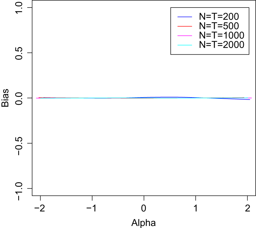
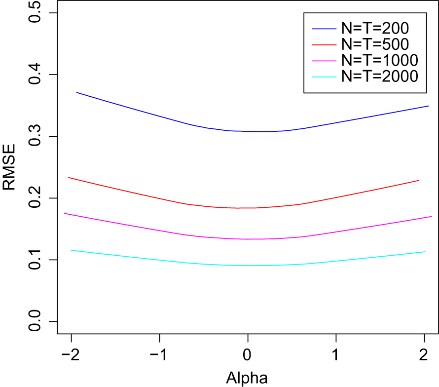
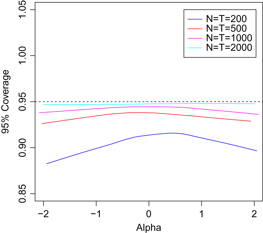
and the right-wing party had an average ideal point of 1. I calculated three quantities—the bias, the root-mean-square error (RMSE), and the coverage of a 95% confidence interval. The bias is the average estimated ideal point across the Monte Carlo datasets, subtracting the true ideal point. The RMSE is the square root of the average error between the estimated and true ideal points. Both of these were used to test whether the estimator was behaving as a consistent estimator—if the estimator is consistent, the bias and RMSE should converge to zero as N and T go to infinity. The coverage of the 95% confidence interval was used to test whether the standard errors were behaving as they should—if the estimates are asymptotically normal and the asymptotic Hessian has been calculated properly, the empirical coverage of a 95% confidence interval should converge to 95% as N and T go to infinity.
 $$ \begin{align} \widehat{Bias}_n = \tfrac{1}{R} \sum_{r=1}^R \left( \hat{\alpha}_{n,r} - \alpha_{n0} \right). \end{align} $$
 $$ \begin{align} \widehat{RMSE}_n = \sqrt{\tfrac{1}{R} \sum_{r=1}^R \left( \hat{\alpha}_{n,r} - \alpha_{n0} \right)^2}. \end{align} $$
 $$ \begin{align} \widehat{Coverage}_n = \tfrac{1}{R} \sum_{r=1}^R \left( 1\{ \hat{\alpha}_{n,r} - 1.96 s^{\alpha}_n \le \alpha_{n0} \le \hat{\alpha}_{n,r} + 1.96 s^{\alpha}_n\} \right). \end{align} $$
The results of the Monte Carlo experiments are given in Figures 1, 2, and 3. The results reported in Figure 1 demonstrate that the bias is very close to zero (relative to the scale of the true ideal points), even for relatively small sample sizes. The results reported in Figure 2 demonstrate that the RMSE becomes smaller and smaller as the sample size increases. The results reported in Figure 3 demonstrate that the empirical coverage gets closer and closer to 95% as the sample size increases. Even for small sample sizes, the coverage is very close to 95% for ideal points near the center of the distribution, while for more extreme ideal points, there is a small amount of undercoverage. Overall, these results suggest that the estimator and its associated standard errors perform well. To be clear, I am not suggesting that alternative estimators—such as wnominate, ideal, and emIRT—perform poorly. Existing Monte Carlo evidence suggests they perform well and the evidence I present in the next section demonstrates that all these estimators produce very similar estimates when they properly converge.
Monte Carlo estimates of bias for the ipe estimator.

Monte Carlo estimates of the root-mean-square error for the ipe estimator.

Monte Carlo estimates of 95% coverage for the ipe estimator—the dashed line represents correct coverage.

5.2 Small-Scale Applications
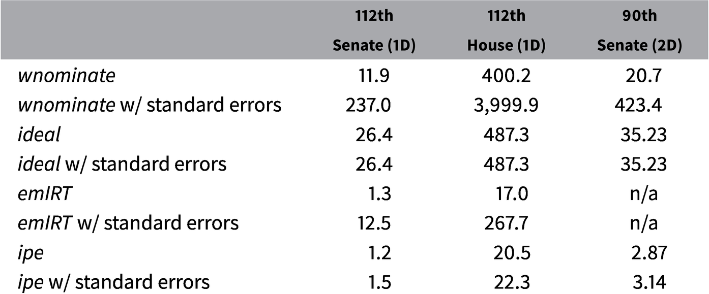
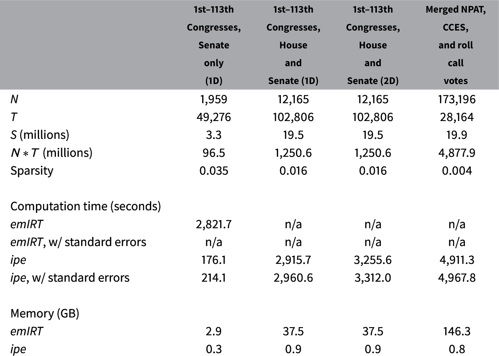
I applied my method as well as the three existing methods to a number of applications. I begin by comparing my method to wnominate, ideal, and emIRT on a number of small-scale applications. I first consider small-scale applications, because wnominate and ideal either cannot handle large-scale applications or will require excessive computation time on these applications. These small-scale applications are enough to illustrate the similarity of the results produced by the methods when they converge properly and to illustrate the advantage of my method over wnominate and ideal in computation time (Table 1). The next subsection will consider increasing challenging applications, demonstrating that my estimator can handle applications that existing estimators cannot.
Computation time (in seconds) for small-scale applications.

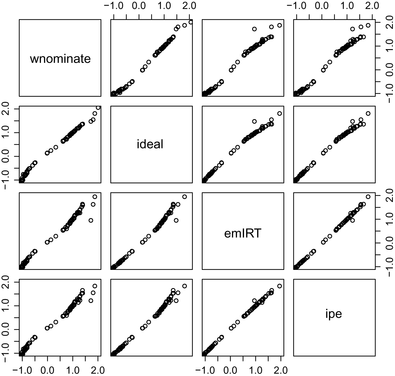
The first example involves estimating a one-dimensional model applied to the 112th Senate. Figure 4 compares the ideal points estimated using the four different methods. As can be seen, the four methods produce very similar estimates. Table 2 reports the computation time for each of the methods, for this and a number of other applications. ipe performed best, requiring 1.2 and 1.5 seconds without and with standard errors, respectively. If one is not interested in standard errors, emIRT was very quick, requiring 1.3 seconds. wnominate required 11.9 seconds. The computation time of ideal depends on the number of Markov chain iterations. I choose to run ideal for 5,000 iterations, with the first 2,500 being burn-in. This is a smaller number of iterations than is used in published work, and more iterations will lead to longer computation times. To emphasize the advantages of ipe, I choose to use a number of iterations at the low end, since even at this low end, my approach preforms favorably. I found that ideal took 26.4 seconds. When standard errors were required, wnominate and emIRT took considerably longer. In timing these methods, I assumed a very low number of bootstrap replications—20. Lewis and Poole (Reference Lewis and Poole2004) and Imai et al. (Reference Imai, Lo and Olmsted2016) used 1,000 replications in their published work. Even with this very low number of bootstrap replications, I found that emIRT required 12.5 seconds and wnominate required 237.0 seconds.
Estimated ideal points for the 112th Senate.

Computation time (in seconds) for small-scale applications.

Abbreviations: CCES, Cooperative Congressional Election Study; NPAT, National Political Awareness Test.
I next applied all the methods to a larger chamber—the 112th House. When no standard errors were required, emIRT was the quickest, requiring 17.0 seconds. ipe required 20.5 seconds. ideal and wnominate took much longer. When standard errors were desired, ipe was the quickest, requiring 22.3 seconds. emIRT took more than 10 times as long, with ideal slower and wnominate requiring over an hour.
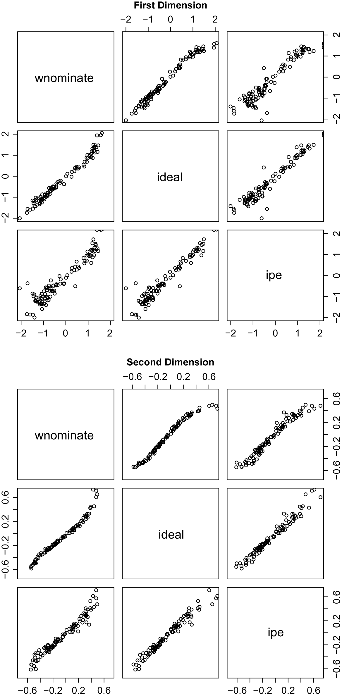
I next applied three of the methods to estimate two-dimensional ideal points for the 90th Senate (emIRT does not support estimating ideal points in more than one dimension).Footnote
9
Figure 5 compares the estimates. To make the estimates comparable, a common normalization must be chosen. I normalized the ideal points, so that the mean Republican was located at (1,0), the mean non-Southern Democrat was located at (
 $-1,-0.25$
), and the mean Southern Democrat was located at (
 $-0.6,0.25$
). The three methods produce similar estimates with one important difference—wnominate imposes the constraint that the ideal points lie in the unit circle and this leads to some Democratic ideal points bunching up against the border of the unit circle. In terms of computation time, ipe was the fastest method by a significant margin.
Estimated two-dimensional ideal points for the 90th Senate.

To summarize the results on the small-scale applications, when standard errors are not required, ipe and emIRT are competitive. When standard errors are required, ipe is much more computationally efficient, and beats the alternative methods in all cases by a factor greater than 10, even when generous assumptions are made with respect to the number of bootstrap replications and the number of Markov chain iterations. It should be noted that while it appears that emIRT dominates ideal when standard errors are required, one could argue that the assumption of 20 bootstrap replications is too generous to emIRT. If one left the number of Markov chain iterations for ideal unchanged and raised the number of bootstrap replications for emIRT to 100, ideal would be more computationally efficient when standard errors are required. In addition, the computation time will have some sensitivity to the convergence criterion used.Footnote 10
5.3 Large-Scale Applications
I next turn to some more difficult problems. The first such application estimates the ideal points of Senators who served in the 1st through the 113th Congresses. I follow the approach taken by Poole’s DWCS and use as bridge voters Senators who served in more than one congress.Footnote
11
The resulting data matrix contains
 $N=1,959$
voters and
 $T=49,276$
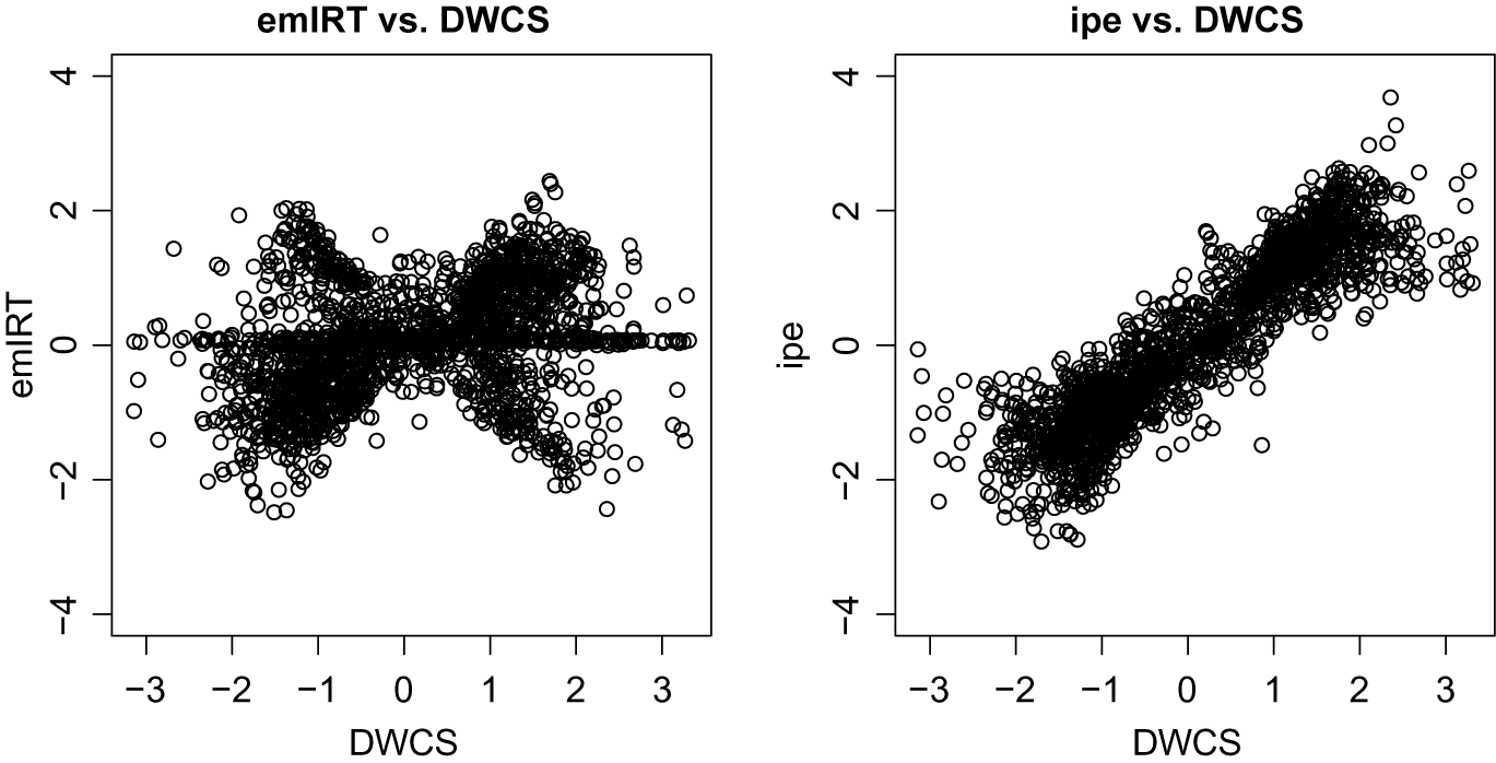
votes, with 97 million entries, of which 3 million are nonmissing. I applied only emIRT and ipe, because wnominate and ideal would take excessively long to run. I used random starting values for emIRT, because this software does not include an approach for identifying good starting values. For ipe, I applied the approach developed in Section A.1. Figure 6 reports the scatter plots between the two estimators and the DWCS. There is a strong correspondence between the ideal points estimated by ipe and the DWCS indicating that my method of estimating the ideal points, combined with my method of generating starting values, is effective in this application.
Scatter plot of ideal points of Senators who served in the 1st through 113th Congresses.

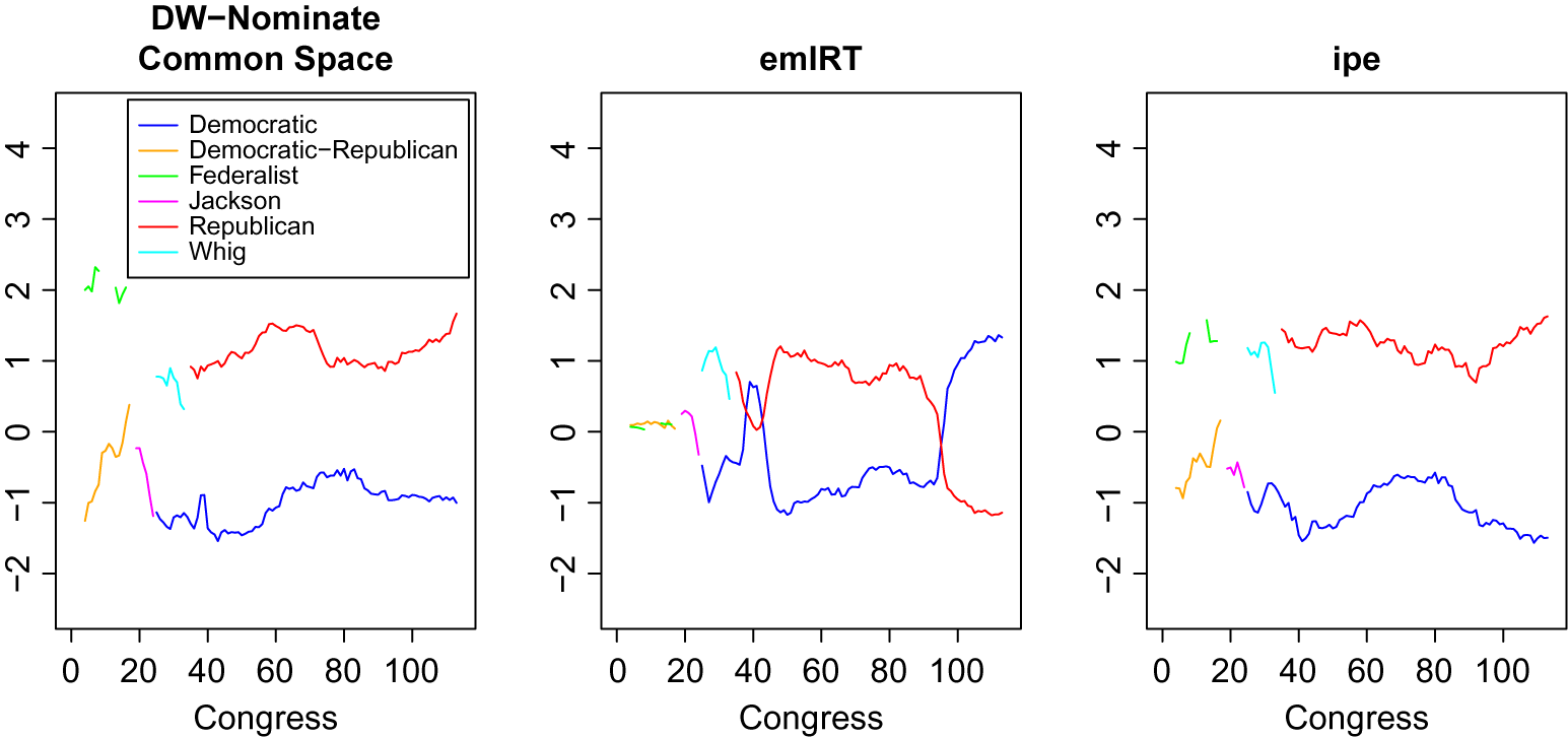
The results for emIRT do not appear to converge properly. The resulting estimates are presented in Figures 6 and 7. The estimates are barely correlated with the DWCS and the ipe results. I note that Imai et al. (Reference Imai, Lo and Olmsted2016) do not claim that their method performs well on such applications without proper starting values. Instead, when they did apply their approach to estimate dynamic ideal points for the U.S. House, they applied the same starting values used by Poole and Rosenthal (Reference Poole and Rosenthal1997) in computing the DWCS . These starting values were in turn computed over time using experimentation—Poole has referred to himself as the “outer loop,” adjusting the starting values when the results did not appear to converge properly. I also note that emIRT may converge properly if one is lucky with the random starting values. I believe it is appropriate to compare my method to emIRT with random starting values, because borrowing the starting values—as Imai et al. (Reference Imai, Lo and Olmsted2016) do—would not be available to scholars in other applications, so this comparison better captures the performance of the two methods in new applications that may emerge. Moreover, even for this application, an automatic way of deriving starting values is an improvement over the experimentation that was used to arrive at the starting values for the DWCS . Figure 7 demonstrates where the convergence problems come from—the algorithm gets stuck in a local maximum where certain sessions of Congress have the wrong left–right orientation relative to other sessions.Footnote 12 This problem is common to emIRT, ipe, and Poole and Rosenthal’s (Reference Poole and Rosenthal1997) various estimators, and a similar problem can lead Bayesian samplers to become trapped in a local mode of the posterior.
Party means for Senators who served in the 1st through 113th Congresses.

Beyond the problem of proper convergence, ipe is faster than emIRT. My method required 176 seconds to compute without standard errors and 214 seconds to compute with standard errors. emIRT required 2,821.7 seconds to compute without standard errors. If standard errors were desired, emIRT would require many multiples of this.
I next consider an even more challenging application—ideal points for members of the House and Senate for the 1st through 113th Congresses. In this case, there are
 $N=12,165$
voters and
 $T=102,806$
votes. The resulting data matrix includes 1.3 billion entries, of which 19 million are nonmissing. Because of the large data matrix, applying emIRT is not feasible. Experimenting on smaller problems, I found that emIRT required approximately 30 bytes to store each observation, meaning that applying it to this dataset would require 38 gigabytes of memory, which is more than any computer I have access to. Beyond the infeasibility, extrapolating from the results on the dynamic U.S. Senate suggests that computing the estimates would require excessive time, particularly if standard errors were desired. The fact that ipe is able to avoid storing missing votes in the data matrix means that it avoids this problem. The entire process of computing starting values, estimating the ideal points, and computing the standard errors required about 40 minutes. I similarly applied ipe to estimate two-dimensional ideal points for the 1st through 113th U.S. House and Senate. ipe again performed well, requiring 55 minutes to compute the estimates.
The next application was designed to test estimation where the chambers are held together by bridge votes. I estimated ideal points of members of the House and Senate for the 103rd through 114th Congresses, House and Senate candidates who had coded responses to the 1992–2016 National Political Awareness Test (NPAT), and survey respondents from the 2006, 2008, 2010, 2012, and 2014 Cooperative Congressional Election Studies (CCESs). Legislators and legislative candidates were allowed to have different ideal points in different years, and bridge votes are used to connect the various chambers. Four types of bridge votes were used, including (i) identical roll call votes in the U.S. House and Senate, (ii) identical NPAT questions that appeared in multiple years, (iii) identical CCES questions that appeared in multiple years, and (iv) CCES questions that asked respondents to take positions on roll call votes. This is probably the most challenging application I consider—there are
 $N = 173,196$
voters and
 $T = 28,164$
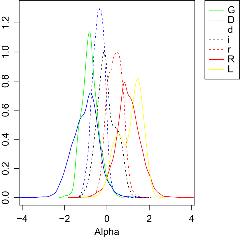
votes. The data matrix has 4.9 billion entries, of which 19 million are nonmissing. Here again, emIRT is not feasible—I estimated that the memory requirements alone would be 146 gigabytes. Because ipe does not require storing the dense matrix, the memory requirements are much lower—approximately 0.8 gigabytes. The computation time for ipe was 83 minutes in total (including the computation of standard errors). Of this, approximately 56 seconds were used to compute the standard errors and 26 minutes were used for computing the starting values. Figure 8 reports the density of the estimated ideal points.
Estimated ideal points for legislators, legislative candidates, and Cooperative Congressional Election Study (CCES) respondents—d, i, and r denote Democratic, independent, and Republican respondents to the CCES, and D, R, L, and G denote Democratic, Republican, Libertarian, and Green legislators or legislative candidates. The analysis includes individuals for which at least 10 votes were available.

6 Conclusion
In this paper, I introduced a set of techniques for large-scale ideal point estimation, designed to overcome a number of limitations of existing methods. My method is computationally fast, is able to efficiently deal with sparse data matrices, is able to efficiently compute standard errors, and is able to generate starting values automatically.
The methods I introduce here hold promise in related ideal point problems and nonlinear panel data models more generally. The estimation approach I developed can be applied to any M-Estimator with fixed effects. My result on the asymptotic Hessian may extend to this general framework as well. The approaches for computing starting values could be applied to other ideal point problems including ones considered in Slapin and Proksch (Reference Slapin and Proksch2010), Peress and Spirling (Reference Peress and Spirling2010), Bonica (Reference Bonica2013), Peress (Reference Peress2013), Bonica (Reference Bonica2014), and Barbera (Reference Barbera2015).
Acknowledgments
I would like to thank James Lo as well as three anonymous reviewers for helpful comments on this paper.
Data Availability Statement
The replication materials for this paper can be found in Peress (Reference Peress2020) or the Harvard Dataverse at http://doi.org/10.7910/DVN/P5SIO1.
Supplementary Material
For supplementary material accompanying this paper, please visit http://doi.org/10.1017/pan.2021.5.