1 Introduction
Marine and coastal structures may often operate in harsh sea environments and be exposed to violent water wave impacts. This concern is especially relevant today where the world is facing an increase in the number and severity of extreme natural events that directly influence the sea state. When these structures interact with a violent wave field, several loading scenarios may occur, such as impulsive wave attack (e.g. sloshing) or the impact of a focused wave group. These loading scenarios may cause serious structural damage and even structural failure, and thus they may endanger human lives (Nikolkina & Didenkulova Reference Nikolkina and Didenkulova2011). Therefore, it is essential to accurately model the interaction between violent wave fields and structures, so that the hydrodynamic loading and the corresponding structural response are properly assessed.
In practice, wave–structure interaction problems for marine and coastal applications are usually modelled by assuming that the structure is perfectly rigid (see Faltinsen Reference Faltinsen1993). This allows one to perform separate analyses to predict the hydrodynamic loads and the corresponding structural response. In many cases, the characteristic time period of the impacting waves is much longer than the characteristic time period of the elastic response. In such conditions, separate analyses are reasonable (Newman Reference Newman1994). However, in violent interaction scenarios and especially when the structure is relatively flexible, hydroelastic effects can have a decisive role in predicting the hydrodynamic loads and the corresponding elastic response (see e.g. Faltinsen Reference Faltinsen2000; Faltinsen & Timokha Reference Faltinsen and Timokha2009; Korobkin, Părău & Vanden-Broeck Reference Korobkin, Părău and Vanden-Broeck2011), and therefore must be taken into account. In order to account for hydroelasticity, a coupled model of interaction is needed and a coupled analysis must be performed.
Most of the hydroelastic models that are found in the open literature are devoted to floating structures, as these can be utilized for many important applications such as very large floating structures (Watanabe, Utsunomiya & Wang Reference Watanabe, Utsunomiya and Wang2004) or ice floes (Squire Reference Squire2007). Models for vertical fixed structures are quite rare. Nevertheless, these models are important for several fundamental applications, such as wind turbines (Marino, Lugni & Borri Reference Marino, Lugni and Borri2013), flexible breakwaters (Wang & Ren Reference Wang and Ren1993; Kumar & Sahoo Reference Kumar and Sahoo2006; Behera, Mandal & Sahoo Reference Behera, Mandal and Sahoo2013), energy convertors (Xie, Wang & Wu Reference Xie, Wang and Wu2014), liquefied natural gas (LNG) tanks (Malenica et al. Reference Malenica, Korobkin, Scolan, Gueret, Delafosse, Gazzola, Mravak, Chen and Zalar2006; Ten, Malenica & Korobkin Reference Ten, Malenica and Korobkin2011; Lugni et al. Reference Lugni, Bardazzi, Faltinsen and Graziani2014) and cylindrical piles (Choi, Lee & Gudmestad Reference Choi, Lee and Gudmestad2015).
The few available models for hydroelastic interaction between vertical structures and water waves are categorized into analytical models (e.g. He & Kashiwagi Reference He and Kashiwagi2009; Korobkin, Stukolov & Sturova Reference Korobkin, Stukolov and Sturova2009; Peter & Meylan Reference Peter and Meylan2010), which are typically limited to linear wave theory, semi-analytical models (e.g. Ten et al. Reference Ten, Malenica and Korobkin2011), which can only be used to study specific impact scenarios, and numerical models, which are more general and can consider the impact of an arbitrary and nonlinear wave field. The advantages of numerical models make them the most suitable for hydroelastic analyses of vertical structures under various interaction scenarios. On the other hand, they commonly demand considerable computational power and long computation times.
Most of the models that have already been proposed are based on coupling of a solution method for the fluid and a solution method for the structure. The latter is most commonly the finite element method (FEM). For the solution of the fluid motion, several methods have been proposed, for example, the boundary element method (BEM) (He & Kashiwagi Reference He and Kashiwagi2009, Reference He and Kashiwagi2012), the finite differences method (FDM) (Liao & Hu Reference Liao and Hu2013) and particle methods such as the meshless local Petrov–Galerkin (MLPG) method (Sriram & Ma Reference Sriram and Ma2012) and smooth particle hydrodynamics (SPH) (Antoci, Gallati & Sibilla Reference Antoci, Gallati and Sibilla2007).
Although promising, these numerical approaches mostly address the fully coupled hydroelastic solution through an iterative process in each time step. Together with the requirement for nonlinear solution of the fluid, and perhaps the structure, the numerical approach becomes very expensive in terms of computational time. This problem is particularly relevant to particle methods (e.g. SPH), which are so time-consuming that it is not feasible to use them for hydroelastic problems that require large domains, long interaction times, or repeated simulations for parametric investigation or statistical purposes. On the other hand, the particle methods are suitable for studying rapid and extremely severe hydroelastic interactions in complex domains.
When the considered problem is formulated in a simple domain, global interpolant functions can be utilized for the nonlinear solution of the fluid, and can significantly reduce the computational time. Therefore, for such problems, a numerical method that is based on global interpolant functions can be used to study certain phenomena which may only be captured in investigations involving long fluid–structure interaction time or repeated simulations.
In the present paper, such a method is first suggested for the fundamental problem of the interaction of a nonlinear wave field over constant depth and an elastic wall. The approach proposed here is based on two spectral methods. For the solution of the fluid, the high-order spectral method (HOSM) is used (Dommermuth & Yue Reference Dommermuth and Yue1987; West et al. Reference West, Brueckner, Janda, Milder and Milton1987), whereas the mode expansion method (MEM) is used to solve the motion of the wall (Han, Benaroya & Wei Reference Han, Benaroya and Wei1999). The formulation of the coupled method is detailed in § 2 for two basic cases: a rigid wall supported by elastic springs, and a deformable elastic wall. The first case represents a model problem where the deformability of the wall is reflected by a single degree of freedom. The second problem represents the general continuous case of an elastic deformable wall. The verification of the method and its ability to model the hydroelastic interaction of a rigid wall supported by springs and an incoming wave field is considered in § 3. In the same section, the method is used to gain further insight into the phenomenon of hydrodynamic amplification that occurs as a result of structural elastic response to an impulsive wave impact. This phenomenon has been recently reported by Lugni et al. (Reference Lugni, Bardazzi, Faltinsen and Graziani2014) and Choi et al. (Reference Choi, Lee and Gudmestad2015), and it contradicts the anticipated relaxation results (Malenica et al. Reference Malenica, Korobkin, Scolan, Gueret, Delafosse, Gazzola, Mravak, Chen and Zalar2006; He & Kashiwagi Reference He and Kashiwagi2012). To this end, § 3 also concerns a parametric investigation which studies the influence of the wall’s dynamics on the maximum wave run-up and wave force due to an impulsive wave impact. In § 4, the method is verified for the hydroelastic interaction with a continuously deformable elastic wall. Then, it is used to investigate the hydroelastic response of the deformable wall due to the impact of a nonlinear wave group. Special attention is drawn to the effect of the nonlinear group evolution on the interaction of the incoming waves with the deformable wall, aiming to extend recent results of this effect which have been found for the interaction with a fixed wall (Akrish, Rabinovitch & Agnon Reference Akrish, Rabinovitch and Agnon2016a ; Akrish et al. Reference Akrish, Schwartz, Rabinovitch and Agnon2016b ). Finally, conclusions are drawn in § 5.
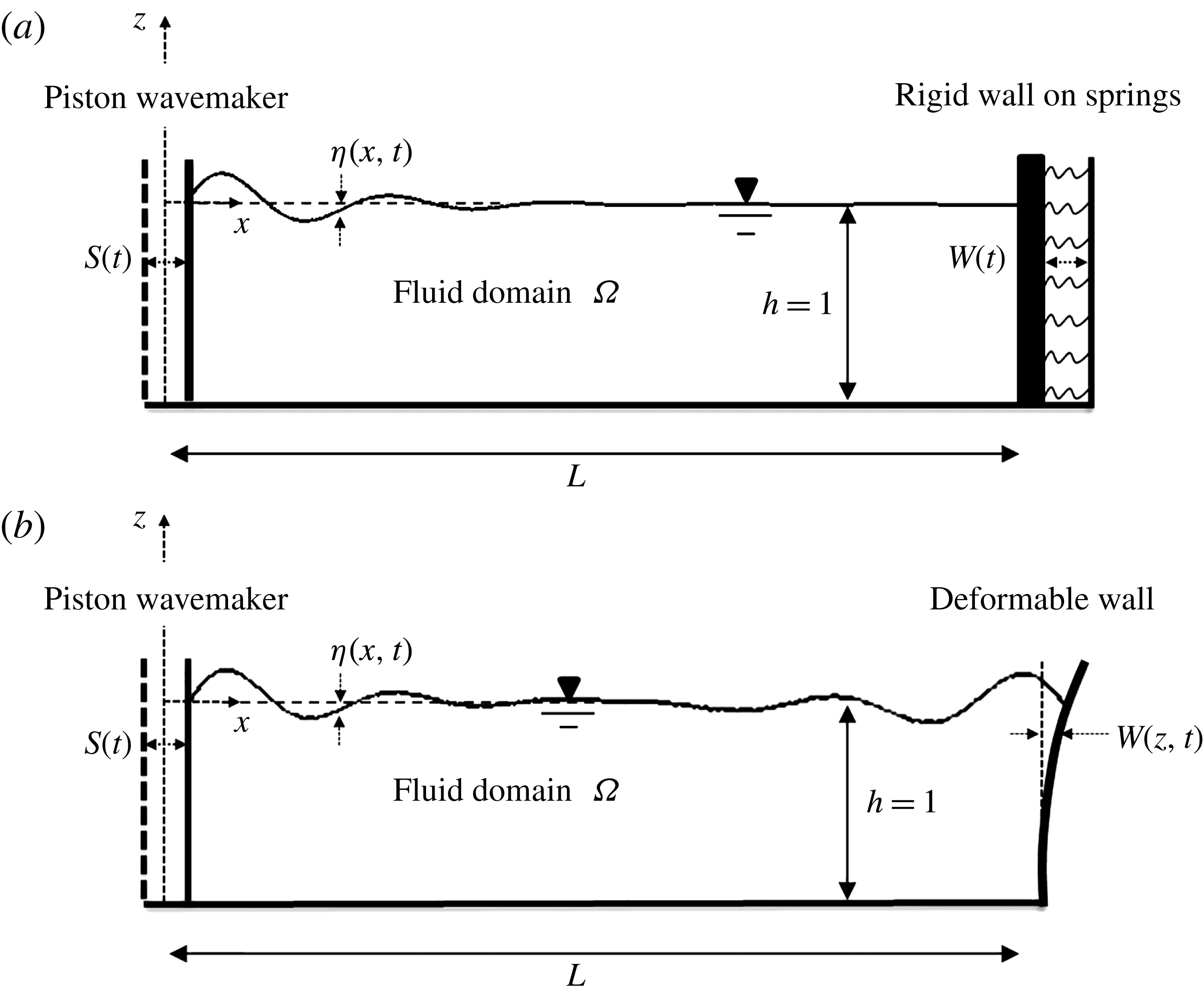
Models of the numerical wave flume: the notation, geometry and coordinates. (a) The interaction model of water waves and a rigid wall supported by lateral springs. (b) The interaction model of water waves and a deformable wall.

2 A spectral method for hydroelastic problems
2.1 Mathematical formulation
The two-dimensional hydroelastic problems considered here are illustrated in figure 1. For both problems, a Cartesian coordinate system with the origin located at the intersection of the wavemaker and the mean water level is adopted. The vertical axis,
 $z$
, is oriented upwards and the horizontal axis,
 $x$
, is oriented towards the elastic wall, which is located at the end of each of the illustrated flumes. The vertical and horizontal dimensions of the flumes are denoted by
 $h$
and
 $L$
, whereas
 $\unicode[STIX]{x1D702}$
,
 $S$
and
 $W$
represent the displacement functions of the water surface, the wavemaker and the elastic wall, respectively. Water waves are simulated along the flume using Euler’s equations, which are derived by assuming incompressible fluid and inviscid flow. These assumptions, together with the assumption of irrotational flow, successfully describe the water behaviour under nonlinear surface waves (Dommermuth et al.
Reference Dommermuth, Yue, Lin, Rapp, Chan and Melville1988; Bonnefoy, Le Touzé & Ferrant Reference Bonnefoy, Le Touzé and Ferrant2006). Applying the definition of a velocity potential,
 $\boldsymbol{u}=\unicode[STIX]{x1D735}\unicode[STIX]{x1D719}$
, the irrotational Euler system can be expressed as follows:
 $$\begin{eqnarray}\displaystyle & \displaystyle \unicode[STIX]{x1D6FB}^{2}\unicode[STIX]{x1D719}=0,\quad \text{in}~\unicode[STIX]{x1D6FA}, & \displaystyle\end{eqnarray}$$
 $$\begin{eqnarray}\displaystyle & \displaystyle \unicode[STIX]{x1D70C}_{w}\,\unicode[STIX]{x2202}_{t}\unicode[STIX]{x1D719}+{\textstyle \frac{1}{2}}\unicode[STIX]{x1D70C}_{w}((\unicode[STIX]{x2202}_{x}\unicode[STIX]{x1D719})^{2}+(\unicode[STIX]{x2202}_{z}\unicode[STIX]{x1D719})^{2})+\unicode[STIX]{x1D70C}_{w}gz+p=0,\quad \text{in}~\unicode[STIX]{x1D6FA}, & \displaystyle\end{eqnarray}$$
where
 $\boldsymbol{u}$
is the water velocity field,
 $\unicode[STIX]{x1D6FA}$
denotes the physical domain of the flume,
 $\unicode[STIX]{x1D70C}_{w}$
is the water mass density,
 $g$
is the gravitational acceleration,
 $p$
is the fluid pressure and
 $\unicode[STIX]{x1D719}$
is the velocity potential. Equations (2.1) and (2.2) express the requirements for mass and momentum conservation in the flume’s domain. These requirements are accompanied by the following kinematic conditions on the boundaries of the flume:
 $$\begin{eqnarray}\displaystyle & \displaystyle \unicode[STIX]{x2202}_{x}\unicode[STIX]{x1D719}=\unicode[STIX]{x2202}_{t}S,\quad \text{on}~x=0, & \displaystyle\end{eqnarray}$$
 $$\begin{eqnarray}\displaystyle & \displaystyle \unicode[STIX]{x2202}_{z}\unicode[STIX]{x1D719}=0,\quad \text{on}~z=-h, & \displaystyle\end{eqnarray}$$
 $$\begin{eqnarray}\displaystyle & \displaystyle \unicode[STIX]{x2202}_{x}\unicode[STIX]{x1D719}=\unicode[STIX]{x2202}_{t}W,\quad \text{on}~x=L, & \displaystyle\end{eqnarray}$$
 $$\begin{eqnarray}\displaystyle & \displaystyle \unicode[STIX]{x2202}_{t}\unicode[STIX]{x1D702}=\unicode[STIX]{x2202}_{z}\unicode[STIX]{x1D719}-\unicode[STIX]{x2202}_{x}\unicode[STIX]{x1D719}\unicode[STIX]{x2202}_{x}\unicode[STIX]{x1D702},\quad \text{on}~z=\unicode[STIX]{x1D702}(x,t), & \displaystyle\end{eqnarray}$$
where (2.3) represents the movement of the piston wavemaker as illustrated in figure 1, (2.4) is a no-vertical-flow condition on the fixed bottom of the flume, (2.5) is the linear kinematic condition on the wall’s surface and (2.6) is the kinematic condition on the free surface. Note that, unlike
 $S$
, the motion of the wall,
 $W$
, can be a function of
 $z$
. The two latter conditions consist of two additional unknown functions, namely,
 $\unicode[STIX]{x1D702}$
and
 $W$
. In order to obtain a solution for
 $\unicode[STIX]{x1D719}$
,
 $\unicode[STIX]{x1D702}$
and
 $W$
, two additional equations are required. The first of these two is given by the dynamic condition,
 $$\begin{eqnarray}\displaystyle & \displaystyle \unicode[STIX]{x2202}_{t}\unicode[STIX]{x1D719}=-{\textstyle \frac{1}{2}}(\unicode[STIX]{x2202}_{x}\unicode[STIX]{x1D719}^{2}+\unicode[STIX]{x2202}_{z}\unicode[STIX]{x1D719}^{2})-\,g\unicode[STIX]{x1D702},\quad \text{on}~z=\unicode[STIX]{x1D702}(x,t), & \displaystyle\end{eqnarray}$$
which is derived by neglecting surface tension effects and assuming that the pressure equals zero. The second additional equation is the equation of motion for the elastic wall. For the case of the rigid wall supported by a lateral spring it reads
 $$\begin{eqnarray}\displaystyle & \displaystyle M_{s}\unicode[STIX]{x2202}_{tt}W+K_{s}W=-\int _{-h}^{\unicode[STIX]{x1D702}}\left[\unicode[STIX]{x1D70C}_{w}\unicode[STIX]{x2202}_{t}\unicode[STIX]{x1D719}+{\textstyle \frac{1}{2}}\unicode[STIX]{x1D70C}_{w}(\unicode[STIX]{x2202}_{x}\unicode[STIX]{x1D719}^{2}+\unicode[STIX]{x2202}_{z}\unicode[STIX]{x1D719}^{2})\right]\,\text{d}z,\quad \text{on}~x=L & \displaystyle\end{eqnarray}$$
and for the elastic flexible wall it reads
 $$\begin{eqnarray}\displaystyle & \displaystyle \unicode[STIX]{x1D70C}_{s}b\,\unicode[STIX]{x2202}_{tt}W+EI\,\unicode[STIX]{x2202}_{zzzz}W=-\unicode[STIX]{x1D70C}_{w}\unicode[STIX]{x2202}_{t}\unicode[STIX]{x1D719}-{\textstyle \frac{1}{2}}\unicode[STIX]{x1D70C}_{w}(\unicode[STIX]{x2202}_{x}\unicode[STIX]{x1D719}^{2}+\unicode[STIX]{x2202}_{z}\unicode[STIX]{x1D719}^{2}),\quad \text{on}~x=L, & \displaystyle\end{eqnarray}$$
where
 $M_{s}$
and
 $K_{s}$
stand for the total mass of the rigid wall and the total spring stiffness, both per unit width, while
 $\unicode[STIX]{x1D70C}_{s}b$
and
 $EI$
are the uniformly distributed mass per unit area and bending stiffness of the deformable wall per unit width (
 $b$
is the thickness of the wall, thus
 $I=b^{3}/12$
, and
 $E$
is the wall’s elastic modulus). Equation (2.8a
) is a one-dimensional spring model, while (2.8b
) is the Euler–Bernoulli beam model, which is derived based on certain simplifying assumptions (e.g. the cross-section of the beam remains planar and normal to the deformed axis). Note that the Euler–Bernoulli beam model predicts well the dynamical behaviour of relatively slender beams. But, as a consequence of its underlying assumptions, it disregards several effects (e.g. shear deformations and rotary inertia) that become significant for non-slender beams (Han et al.
Reference Han, Benaroya and Wei1999). In such cases, alternative models such as Timoshenko’s first-order shear deformation theory or higher-order beam theories may be considered. The right-hand side of (2.8a
) is the dynamic fluid force (excluding the hydrostatic contribution at rest) and the right-hand side of (2.8b
) is the dynamic fluid pressure. Finally, the edge conditions of the deformable wall should be specified as well. For a fixed–free wall (see figure 1)
 $$\begin{eqnarray}\displaystyle \left.\begin{array}{@{}l@{}}W=0,\quad \unicode[STIX]{x2202}_{z}W=0,\quad \text{on}~z=-h,\\[2.0pt] \unicode[STIX]{x2202}_{zz}W=0,\quad \unicode[STIX]{x2202}_{zzz}W=0,\quad \text{on}~z=\unicode[STIX]{x1D6E4},\end{array}\right\} & & \displaystyle\end{eqnarray}$$
and for a fixed–fixed wall
 $$\begin{eqnarray}\displaystyle \left.\begin{array}{@{}l@{}}W=0,\quad \text{on}~z=-h,\unicode[STIX]{x1D6E4},\\[2.0pt] \unicode[STIX]{x2202}_{z}W=0,\quad \text{on}~z=-h,\unicode[STIX]{x1D6E4},\end{array}\right\} & & \displaystyle\end{eqnarray}$$
where
 $\unicode[STIX]{x1D6E4}$
represents the height of the wall above the level of the free water surface at rest. In order to obtain a time-dependent solution for
 $\unicode[STIX]{x1D719}$
,
 $\unicode[STIX]{x1D702}$
and
 $W$
, an initial condition for each of these quantities is required:
 $$\begin{eqnarray}\displaystyle & \displaystyle \unicode[STIX]{x1D719}(x,z,t=0)=\unicode[STIX]{x1D719}^{0}(x,z), & \displaystyle\end{eqnarray}$$
 $$\begin{eqnarray}\displaystyle & \displaystyle \unicode[STIX]{x1D702}(x,t=0)=\unicode[STIX]{x1D702}^{0}(x), & \displaystyle\end{eqnarray}$$
for the rigid wall on springs
 $$\begin{eqnarray}\displaystyle & \displaystyle W(t=0)=W^{0} & \displaystyle\end{eqnarray}$$
and for the deformable wall
 $$\begin{eqnarray}\displaystyle & \displaystyle W(z,t=0)=W^{0}(z). & \displaystyle\end{eqnarray}$$
The initial condition of the wall’s velocity is implicitly taken into account through (2.5) and (2.11a
). This completes the formulation of the mathematical model which is implemented in this study in a non-dimensional form. The constant fluid depth
 $h$
, the water mass density
 $\unicode[STIX]{x1D70C}_{w}$
and the gravitational acceleration
 $g$
are used to scale the variables. The solution of the model, which consists of the governing equations for the fluid (2.1) and (2.2), together with the governing equation for the wall (2.8), the boundary conditions (2.3)–(2.7), (2.9) and (2.10), and the initial conditions (2.11), is obtained numerically using spectral methods. This solution is presented in the next section.
2.2 The spectral method
2.2.1 Potential decomposition
The proposed spectral method couples the HOSM for the solution of the fluid (Dommermuth & Yue Reference Dommermuth and Yue1987; West et al. Reference West, Brueckner, Janda, Milder and Milton1987) and the MEM for solving the motion of the wall (Han et al. Reference Han, Benaroya and Wei1999). In each of these methods, the spatial solution is approximated using a global interpolant function that is composed of the eigenfunctions of the considered domain. The spatial derivatives of a differential equation are then accurately evaluated by differentiating the interpolant function analytically. Besides accuracy, the proposed method also serves efficiency. Obviously, most of the computational demand arises from the solution of the fluid. Through the original HOSM formulation (Dommermuth & Yue Reference Dommermuth and Yue1987; West et al. Reference West, Brueckner, Janda, Milder and Milton1987), the assumption of a periodic domain allows one to formulate the interpolant function using Fourier functions, and thus the spatial derivatives are efficiently evaluated through the fast Fourier transform (FFT). However, in the present case, the domain is not periodic. Such cases led to the idea of the potential decomposition concept (Agnon & Bingham Reference Agnon and Bingham1999), where the original problem is decomposed into a sum of several problems. The first problem is periodic. This problem is derived by imposing reflecting lateral boundary conditions. The rest of the problems are called the additional problems. These problems satisfy the movable lateral boundary conditions at the wavemaker and at the vertical wall. Such a decomposition technique is allowable due to the linearity of the Laplace equation (2.1). The solution of the present non-periodic problem is therefore expressed as
 $$\begin{eqnarray}\displaystyle & \displaystyle \unicode[STIX]{x1D719}=\unicode[STIX]{x1D719}_{p}+\unicode[STIX]{x1D719}_{wm}+\unicode[STIX]{x1D719}_{vw}, & \displaystyle\end{eqnarray}$$
where the subscripts
 $p$
,
 $wm$
and
 $vw$
stand for periodic, wavemaker and vertical wall, respectively. This approach allows each problem to be solved separately, where the spatial solution of the periodic potential can be represented by classical standing wave solutions. The time-dependent solution is obtained by adding back the three potentials to satisfy the remaining boundary conditions on the free water surface, where the additional solutions are used as forcing terms, and on the elastic wall boundary. In this way, the efficiency that characterizes the original HOSM is preserved for non-periodic problems as well.
2.2.2 The solution for the additional potentials
An additional solution may stand for a wavemaker condition, absorbing layer condition, elastic boundary, etc. In the present study, the additional problems should satisfy the piston wavemaker condition and the elastic wall condition at the lateral boundaries (see figure 1). The formulation of each of these additional problems is derived from the following general one:
 $$\begin{eqnarray}\displaystyle \left.\begin{array}{@{}l@{}}\unicode[STIX]{x1D6FB}^{2}\unicode[STIX]{x1D719}_{a}=0,\quad \text{in}~\unicode[STIX]{x1D6FA},\\ \unicode[STIX]{x2202}_{x}\unicode[STIX]{x1D719}_{a}=\unicode[STIX]{x2202}_{t}S,\quad \text{on}~x=0,\\ \unicode[STIX]{x2202}_{z}\unicode[STIX]{x1D719}_{a}=0,\quad \text{on}~z=-1,\\ \unicode[STIX]{x2202}_{x}\unicode[STIX]{x1D719}_{a}=\unicode[STIX]{x2202}_{t}W,\quad \text{on}~x=L,\end{array}\right\} & & \displaystyle\end{eqnarray}$$
where
 $\unicode[STIX]{x1D719}_{a}=\unicode[STIX]{x1D719}_{wm}+\unicode[STIX]{x1D719}_{vw}$
and the subscript
 $a$
stands for additional. The formulation for
 $\unicode[STIX]{x1D719}_{wm}$
is derived by substituting
 $W=0$
in (2.13), while the formulation for
 $\unicode[STIX]{x1D719}_{vw}$
is derived by substituting
 $S=0$
in (2.13). Following Agnon & Bingham (Reference Agnon and Bingham1999), the solutions of (2.13) and for the case of a rigid boundary (i.e. the wavemaker or the wall on springs) can be achieved with quadratic polynomials. It is well known that the polynomial solutions for the Laplace equation in the current two-dimensional domain are found from the real and imaginary parts of
 $$\begin{eqnarray}\displaystyle & \displaystyle (x+\text{i}z)^{n},\quad n=0,1,2,\ldots . & \displaystyle\end{eqnarray}$$
Confining to
 $n\leqslant 2$
, and applying the lateral and bottom boundaries expressed in (2.13), the additional potential solutions due to the wavemaker and due to the wall on springs are
 $$\begin{eqnarray}\displaystyle & \displaystyle \unicode[STIX]{x1D719}_{wm}=\frac{\unicode[STIX]{x2202}_{t}S}{2L}[(z+1)^{2}-(x-L)^{2}],\quad \text{in}~\unicode[STIX]{x1D6FA}, & \displaystyle\end{eqnarray}$$
 $$\begin{eqnarray}\displaystyle & \displaystyle \unicode[STIX]{x1D719}_{vw}=\frac{\unicode[STIX]{x2202}_{t}W}{2L}[x^{2}-(z+1)^{2}],\quad \text{in}~\unicode[STIX]{x1D6FA}. & \displaystyle\end{eqnarray}$$
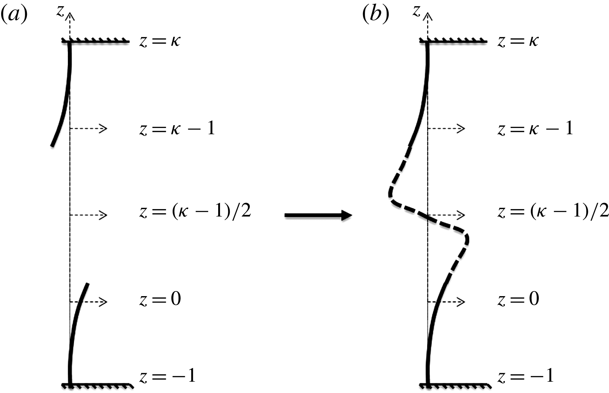
The additional potential corresponding to the case of a deformable wall is obtained following the idea proposed by Bonnefoy et al. (Reference Bonnefoy, Le Touzé and Ferrant2006). The idea is to formulate the additional problem in an extended domain with the following fictitious boundary condition:
 $$\begin{eqnarray}\displaystyle & \displaystyle \unicode[STIX]{x2202}_{z}\unicode[STIX]{x1D719}_{vw}=0,\quad \text{on}~z=\unicode[STIX]{x1D705}, & \displaystyle\end{eqnarray}$$
where
 $\unicode[STIX]{x1D705}$
is chosen according to the following requirements. The first is volume conservation in the extended domain. This is accomplished by asymmetrical extension of the wall boundary (see figure 2). The second is to ensure that the extended wall boundary is smooth enough in order to avoid the Gibbs phenomenon errors. The implementation of these two requirements is described in figure 2, where the free ends in figure 2(a) are interpolated in figure 2(b) by
 $$\begin{eqnarray}\displaystyle & \displaystyle y(z)=-\text{tanh}[r(z-(\unicode[STIX]{x1D705}-1)/2)]. & \displaystyle\end{eqnarray}$$
The coefficient
 $r$
is chosen such that
 $y(z)=1$
at the bottom free end, and
 $y(z)=-1$
at the upper free end. Finally, following the boundary conditions expressed in (2.13) and (2.17), the solution of the additional potential due to the deformable wall can be written as
 $$\begin{eqnarray}\displaystyle \left.\begin{array}{@{}l@{}}\unicode[STIX]{x1D719}_{vw}=\displaystyle \mathop{\sum }_{i=1}^{K}\unicode[STIX]{x1D719}_{vw,i},\\[3.0pt] \unicode[STIX]{x1D719}_{vw,i}=\unicode[STIX]{x2202}_{t}w_{i}\displaystyle \mathop{\sum }_{b=0}^{B}C_{i,b}\cos [\unicode[STIX]{x1D706}_{b}(z+1)]{\displaystyle \frac{\cosh \unicode[STIX]{x1D706}_{b}x}{\cosh \unicode[STIX]{x1D706}_{b}L}},\quad \text{in}~\unicode[STIX]{x1D6FA},\end{array}\right\} & & \displaystyle\end{eqnarray}$$
where
 $w_{i}$
is the time-dependent function that corresponds to the wall’s eigenfunction
 $f_{i}$
, assuming that (in accordance with the MEM) the solution of wall can be written as
 $$\begin{eqnarray}\displaystyle \left.\begin{array}{@{}l@{}}\displaystyle W=\mathop{\sum }_{i=1}^{K}W_{i},\\[3.0pt] \displaystyle W_{i}=w_{i}\,f_{i}.\end{array}\right\} & & \displaystyle\end{eqnarray}$$
The coefficients
 $C_{i,b}$
are obtained through (2.13) to be
 $$\begin{eqnarray}\displaystyle \left.\begin{array}{@{}l@{}}C_{i,b}=-{\displaystyle \frac{\hat{f}_{i,b}}{\unicode[STIX]{x1D706}_{b}\tanh (\unicode[STIX]{x1D706}_{b}L)}},\\[8.0pt] \hat{f}_{i,b}={\displaystyle \frac{2}{\unicode[STIX]{x1D705}+1}}\displaystyle \int _{-1}^{\unicode[STIX]{x1D705}}f_{i}\cos [\unicode[STIX]{x1D706}_{b}(z+1)]\,\text{d}z,\quad b=1,3,5,\ldots .\end{array}\right\} & & \displaystyle\end{eqnarray}$$
Finally,
 $\unicode[STIX]{x1D706}_{b}=b\unicode[STIX]{x03C0}/(1+\unicode[STIX]{x1D705})$
are the standing wavenumbers and
 $B$
,
 $K$
define the number of the wave modes and the number of the wall’s eigenfunctions, respectively.
The method to extend the boundary condition of a wall with an arbitrary vertical shape: (a) asymmetrical extension, (b) smooth interpolation.

Adding back the periodic and the two additional problems, the conditions at the lateral and bottom boundaries of the flume are satisfied. The remaining conditions to satisfy are the free boundary conditions (2.6) and (2.7) and the kinetic wall condition (2.8a ) and (2.8b ).
2.2.3 The numerical solution of the coupled set of equations: the free surface equations and the kinetic wall equation
A fully coupled solution of the free surface equations and the kinetic wall equation is a challenging task. In order to obtain a relatively fast numerical solution of these equations in time, and to capture nonlinear and hydroelastic effects, several approximations are considered. First, the formulation of the HOSM assumes that the values of
 $\unicode[STIX]{x1D719}_{p}$
and
 $\unicode[STIX]{x1D702}$
are small, with a magnitude of
 $O(\unicode[STIX]{x1D700})$
, where
 $\unicode[STIX]{x1D700}$
is a measure of the wave steepness. It is advantageous to formulate these equations in terms of the periodic surface potential
 $\unicode[STIX]{x1D719}_{p}^{s}$
, which is defined as
 $\unicode[STIX]{x1D719}_{p}^{s}=\unicode[STIX]{x1D719}_{p}(x,z=\unicode[STIX]{x1D702},t)$
(Zakharov Reference Zakharov1968). Using this definition and the separate potential representation (2.12), the free surface boundary conditions may be rewritten as
 $$\begin{eqnarray}\displaystyle \left.\begin{array}{@{}l@{}}\unicode[STIX]{x2202}_{t}\unicode[STIX]{x1D702}=V[1+(\unicode[STIX]{x2202}_{x}\unicode[STIX]{x1D702})^{2}]+\unicode[STIX]{x2202}_{z}\unicode[STIX]{x1D719}_{a}-(\unicode[STIX]{x2202}_{x}\unicode[STIX]{x1D719}_{p}^{s}+\,\unicode[STIX]{x2202}_{x}\unicode[STIX]{x1D719}_{a})\unicode[STIX]{x2202}_{x}\unicode[STIX]{x1D702},\\[3.0pt] \unicode[STIX]{x2202}_{t}\unicode[STIX]{x1D719}_{p}^{s}={\textstyle \frac{1}{2}}V^{2}[1+(\unicode[STIX]{x2202}_{x}\unicode[STIX]{x1D702})^{2}]-{\textstyle \frac{1}{2}}(\unicode[STIX]{x2202}_{z}\unicode[STIX]{x1D719}_{a})^{2}-{\textstyle \frac{1}{2}}(\unicode[STIX]{x2202}_{x}\unicode[STIX]{x1D719}_{p}^{s}+\unicode[STIX]{x2202}_{x}\unicode[STIX]{x1D719}_{a})^{2}-\unicode[STIX]{x2202}_{t}\unicode[STIX]{x1D719}_{a}-\unicode[STIX]{x1D702},\end{array}\right\}\quad \text{on}~z=\unicode[STIX]{x1D702}(x,t). & & \displaystyle \nonumber\\ \displaystyle & & \displaystyle\end{eqnarray}$$
Using Zakharov’s formulation leaves the modified free surface equations with the periodic vertical velocity
 $V=\unicode[STIX]{x2202}_{z}\unicode[STIX]{x1D719}_{p}(x,z=\unicode[STIX]{x1D702},t)$
as the only non-free surface component. Owing to its periodicity, this quantity can be evaluated following the original HOSM formulation (Dommermuth & Yue Reference Dommermuth and Yue1987; West et al.
Reference West, Brueckner, Janda, Milder and Milton1987):
 $$\begin{eqnarray}\displaystyle \left.\begin{array}{@{}l@{}}\displaystyle V=\mathop{\sum }_{m=1}^{M}V^{(m)},\\[3.0pt] \displaystyle V^{(m)}=\mathop{\sum }_{j=0}^{m-1}{\displaystyle \frac{\unicode[STIX]{x1D702}^{j}}{j!}}\unicode[STIX]{x2202}_{z^{j+1}}\unicode[STIX]{x1D719}_{p}^{(m-j)}(x,0,t),\quad m=1,2,\ldots ,M,\end{array}\right\} & & \displaystyle\end{eqnarray}$$
where
 $M$
is the order of nonlinearity and
 $\unicode[STIX]{x1D719}_{p}$
can be expressed as
 $$\begin{eqnarray}\displaystyle \left.\begin{array}{@{}l@{}}\displaystyle \unicode[STIX]{x1D719}_{p}=\mathop{\sum }_{m=1}^{M}\unicode[STIX]{x1D719}_{p}^{(m)},\quad A_{n}=\mathop{\sum }_{m=1}^{M}A_{n}^{(m)},\\[6.0pt] \displaystyle \unicode[STIX]{x1D719}_{p}^{(m)}=\mathop{\sum }_{n=0}^{N}A_{n}^{(m)}(t){\displaystyle \frac{\cosh [k_{n}(z+1)]}{\cosh k_{n}}}\cos k_{n}x,\end{array}\right\} & & \displaystyle\end{eqnarray}$$
defined by
 $k_{n}=n\unicode[STIX]{x03C0}/L$
, the wavenumbers, and
 $N$
, the number of wave modes that are considered. In this study, all the simulations are performed with
 $M=8$
, whereas the value of
 $N$
is selected specifically for each simulation. Note that (2.22) also depends on the motion of the wall,
 $W$
, which is governed by (2.8a
) and (2.8b
). In turn, (2.8a
) and (2.8b
) depend on both
 $\unicode[STIX]{x1D719}_{p}$
and
 $\unicode[STIX]{x1D702}$
, which are necessary to calculate the pressure (or the force for the wall on springs case) exerted on the wall. The solution of (2.8b
) (for the deformable wall case) is obtained using the MEM. Through this method, the orthogonality of the wall’s eigenfunctions is used to reduce (2.8b
) to a system of equations. This is done by substituting (2.20) into (2.8b
), multiplying by
 $f_{i}$
and integrating from
 $-1$
to
 $\unicode[STIX]{x1D6E4}$
. The resulting system of equations is given as follows:
 $$\begin{eqnarray}\displaystyle \unicode[STIX]{x1D614}_{eff}\left(\begin{array}{@{}c@{}}\unicode[STIX]{x2202}_{tt}w_{1}\\ \unicode[STIX]{x2202}_{tt}w_{2}\\ \vdots \\ \unicode[STIX]{x2202}_{tt}w_{K}\end{array}\right)+\unicode[STIX]{x1D612}_{eff}\left(\begin{array}{@{}c@{}}w_{1}\\ w_{2}\\ \vdots \\ w_{K}\end{array}\right)=\left(\begin{array}{@{}c@{}}\tilde{F}_{1}\\ \tilde{F}_{2}\\ \vdots \\ \tilde{F}_{K}\end{array}\right). & & \displaystyle\end{eqnarray}$$
The matrices
 $\unicode[STIX]{x1D614}_{eff}$
and
 $\unicode[STIX]{x1D612}_{eff}$
can be written explicitly as
 $$\begin{eqnarray}\displaystyle & \displaystyle \unicode[STIX]{x1D614}_{eff}=\left[\left(\begin{array}{@{}cccc@{}}N_{11}m_{s} & 0 & \cdots \, & 0\\ 0 & N_{22}m_{s} & & \vdots \\ \vdots & & \ddots & 0\\ 0 & \cdots \, & 0 & N_{KK}m_{s}\end{array}\right)+\left(\begin{array}{@{}cccc@{}}\unicode[STIX]{x1D6FF}_{11} & \unicode[STIX]{x1D6FF}_{12} & \cdots \, & \unicode[STIX]{x1D6FF}_{1K}\\ \unicode[STIX]{x1D6FF}_{21} & \unicode[STIX]{x1D6FF}_{22} & & \vdots \\ \vdots & & \ddots & \unicode[STIX]{x1D6FF}_{K-1,K}\\ \unicode[STIX]{x1D6FF}_{K1} & \cdots \, & \unicode[STIX]{x1D6FF}_{K,K-1} & \unicode[STIX]{x1D6FF}_{KK}\end{array}\right)\right], & \displaystyle \nonumber\\ \displaystyle & & \displaystyle\end{eqnarray}$$
 $$\begin{eqnarray}\displaystyle & \displaystyle \unicode[STIX]{x1D612}_{eff}=\left(\begin{array}{@{}cccc@{}}N_{11}k_{s}\unicode[STIX]{x1D6FD}_{1}^{4} & 0 & \cdots \, & 0\\ 0 & N_{22}k_{s}\unicode[STIX]{x1D6FD}_{2}^{4} & & \vdots \\ \vdots & & \ddots & 0\\ 0 & \cdots \, & 0 & N_{KK}k_{s}\unicode[STIX]{x1D6FD}_{K}^{4}\end{array}\right), & \displaystyle\end{eqnarray}$$
where
 $m_{s}=\unicode[STIX]{x1D70C}_{s}b/\unicode[STIX]{x1D70C}_{w}h$
is the non-dimensional mass,
 $k_{s}=EI/\unicode[STIX]{x1D70C}_{w}gh^{4}$
is the non-dimensional stiffness and
 $\unicode[STIX]{x1D6FD}_{i}$
is the
 $i$
th wall’s wavenumber associated with the eigenfunction
 $f_{i}$
. Additionally,
 $N_{i}$
,
 $\unicode[STIX]{x1D6FF}_{ij}$
(the so-called ‘added-mass’ terms) and
 $\tilde{F}_{i}$
are defined by the following:
 $$\begin{eqnarray}\displaystyle \displaystyle N_{ii}=\int _{-1}^{\unicode[STIX]{x1D6E4}}f_{i}\,f_{i}\,\text{d}z, & & \displaystyle\end{eqnarray}$$
 $$\begin{eqnarray}\displaystyle \left.\begin{array}{@{}l@{}}\displaystyle \unicode[STIX]{x1D6FF}_{ij}=\int _{-1}^{\unicode[STIX]{x1D702}}f_{i}\mathop{\sum }_{b}C_{j,b}\cos [\unicode[STIX]{x1D706}_{b}(z+1)]\,\text{d}z\\[3.0pt] \qquad -\displaystyle \int _{-1}^{0}f_{i}\mathop{\sum }_{n=0}^{N}\,p_{j}\,\text{d}z\,-\int _{0}^{\unicode[STIX]{x1D702}}f_{i}\mathop{\sum }_{r}{\displaystyle \frac{z^{r}}{r!}}\unicode[STIX]{x2202}_{z^{r}}p_{j}(L,0,t)\,\text{d}z,\\[8.0pt] \displaystyle p_{j}=\hat{\unicode[STIX]{x1D719}}_{vw,j}{\displaystyle \frac{\cosh k_{n}(z+1)}{\cosh k_{n}}}\cos k_{n}L,\end{array}\right\} & & \displaystyle\end{eqnarray}$$
 $$\begin{eqnarray}\displaystyle \left.\begin{array}{@{}l@{}}\tilde{F}_{i}=-\tilde{F}_{1,i}-{\textstyle \frac{1}{2}}\tilde{F}_{2,i}-\tilde{F}_{3,i}-\tilde{F}_{4,i},\\[4.0pt] \displaystyle \tilde{F}_{1,i}=\int _{-1}^{0}f_{i}\unicode[STIX]{x1D713}\,\text{d}z,\quad \text{on}~x=L,\\[8.0pt] \displaystyle \tilde{F}_{2,i}=\int _{-1}^{0}f_{i}\unicode[STIX]{x2202}_{z}\unicode[STIX]{x1D719}_{p}^{2}\,\text{d}z,\quad \text{on}~x=L,\\[6.0pt] \displaystyle \tilde{F}_{3,i}=\int _{0}^{\unicode[STIX]{x1D702}}f_{i}\left[z+\mathop{\sum }_{r}{\displaystyle \frac{z^{r}}{r!}}\unicode[STIX]{x2202}_{z^{r}}p_{p}(L,0,t)\right]\,\text{d}z,\quad p_{p}=\unicode[STIX]{x1D713}+{\displaystyle \frac{1}{2}}\unicode[STIX]{x2202}_{z}\unicode[STIX]{x1D719}_{p}^{2},\\[8.0pt] \displaystyle \tilde{F}_{4,i}=\int _{-1}^{\unicode[STIX]{x1D702}}f_{i}\unicode[STIX]{x2202}_{t}\unicode[STIX]{x1D719}_{wm}\,\text{d}z,\quad \text{on}~x=L,\end{array}\right\} & & \displaystyle\end{eqnarray}$$
where
 $\unicode[STIX]{x1D713}$
is defined as
 $$\begin{eqnarray}\displaystyle \unicode[STIX]{x1D713}=\mathop{\sum }_{n=0}^{N}\hat{\unicode[STIX]{x1D713}}\frac{\cosh [k_{n}(z+1)]}{\cosh k_{n}}\cos k_{n}x & & \displaystyle\end{eqnarray}$$
and
 $\hat{\unicode[STIX]{x1D713}}$
is essentially the Fourier components of the periodic potential acceleration without the effect of the wall’s acceleration. Accordingly, it is defined as
 $$\begin{eqnarray}\displaystyle \hat{\unicode[STIX]{x1D713}}=\unicode[STIX]{x2202}_{t}A_{n}+\mathop{\sum }_{i=1}^{K}\unicode[STIX]{x2202}_{tt}w_{i}\hat{\unicode[STIX]{x1D719}}_{vw,i}. & & \displaystyle\end{eqnarray}$$
Finally,
 $\hat{\unicode[STIX]{x1D719}}_{vw,j}$
are the Fourier components of the additional function related to
 $f_{j}$
on the free surface. Using the definition in (2.31), all the terms that multiply wall acceleration component,
 $\unicode[STIX]{x2202}_{tt}w_{i}$
, are substituted in the added-mass terms,
 $\unicode[STIX]{x1D6FF}_{ij}$
, at the left side of (2.25). To conclude the presentation of the MEM, it is noted that, due to the orthogonality of the wall’s eigenfunctions,
 $\unicode[STIX]{x1D612}_{eff}$
and the first part of
 $\unicode[STIX]{x1D614}_{eff}$
become diagonal (
 $N_{ij}=0,~i\neq j$
). However, the system is still coupled through the added-mass terms,
 $\unicode[STIX]{x1D6FF}_{ij}$
. For the rigid wall on springs, the wall’s kinetic equation can be written as
 $$\begin{eqnarray}\displaystyle (m_{s}+\unicode[STIX]{x1D6FF})\unicode[STIX]{x2202}_{tt}W+k_{s}W=\tilde{F}, & & \displaystyle\end{eqnarray}$$
where in this case the non-dimensional mass is defined as
 $m_{s}=M_{s}/\unicode[STIX]{x1D70C}_{w}h^{2}$
, and the non-dimensional stiffness is defined as
 $k_{s}=K_{s}/\unicode[STIX]{x1D70C}_{w}gh$
. Here,
 $\unicode[STIX]{x1D6FF}$
is defined by
 $$\begin{eqnarray}\displaystyle \left.\begin{array}{@{}c@{}}\displaystyle \unicode[STIX]{x1D6FF}={\displaystyle \frac{1}{2L}}\left[L^{2}(\unicode[STIX]{x1D702}+1)-\,{\displaystyle \frac{(\unicode[STIX]{x1D702}+1)^{2}}{3}}\right]-\int _{-1}^{0}\mathop{\sum }_{n=0}^{N}\,p\,\text{d}z\,-\int _{0}^{\unicode[STIX]{x1D702}}\mathop{\sum }_{r}{\displaystyle \frac{z^{r}}{r!}}\unicode[STIX]{x2202}_{z^{r}}p(L,0,t)\,\text{d}z,\\[8.0pt] \displaystyle p=\hat{\unicode[STIX]{x1D719}}_{vw}{\displaystyle \frac{\cosh k_{n}(z+1)}{\cosh k_{n}}}\cos k_{n}L,\end{array}\right\} & & \displaystyle\end{eqnarray}$$
and
 $\tilde{F}$
is simply derived by substituting
 $f_{i}=1$
into (2.29).
The implementation of (2.8a
) and (2.8b
), through (2.25) and (2.32), respectively, introduces further simplifying assumptions. One assumption is that the run-up on the wall is lower than the wall’s height. An additional assumption suggests that the contribution of products containing the additional potentials for the computation of
 $\tilde{F}$
(e.g.
 $\unicode[STIX]{x2202}_{z}\unicode[STIX]{x1D719}_{wm}^{2}$
,
 $\unicode[STIX]{x2202}_{z}\unicode[STIX]{x1D719}_{vw}^{2}$
,
 $\unicode[STIX]{x2202}_{z}\unicode[STIX]{x1D719}_{vw}\unicode[STIX]{x2202}_{z}\unicode[STIX]{x1D719}_{p}$
) are negligible, and therefore are omitted.
This completes the implementation of the present spectral method, which can be summarized with the following steps: Decompose the problem into the periodic and the additional problems, and derive their spatial solutions. Then, the problems are added back to satisfy the free boundary conditions, where the additional derivatives serve as forcing terms, and the kinetic condition on the wall, where the components that explicitly depend on the wall acceleration are introduced into the added-mass terms,
 $\unicode[STIX]{x1D6FF}$
. Next, the spatial derivatives for
 $\unicode[STIX]{x1D719}_{p}^{s}$
and
 $\unicode[STIX]{x1D702}$
at each time step are efficiently computed utilizing the FFT algorithm (following the HOSM), and in the case of the deformable wall, the spatial derivative is performed analytically by differentiating the wall’s eigenfunction (following the MEM). Finally, the spatially discretized coupled set of equations for solving
 $\unicode[STIX]{x1D719}_{p}^{s}$
,
 $\unicode[STIX]{x1D702}$
and
 $W$
are marched in time using the classical fourth-order Runge–Kutta (RK4) scheme.
In the following, the present spectral method is used to study two scenarios. First, the method is used to study the interaction of a rigid wall supported by lateral springs and a pulse-type water wave. Then, the method is used to investigate the interaction of a continuously deformable wall and an incident wave group. Recall once again that this study is implemented in a non-dimensional form (the representative dimensions are given in § 2). Additionally, note that in the following the results are also normalized by the initial hydrodynamic parameters.
3 Hydroelastic interaction of a rigid wall supported by springs and a pulse-type wave
A rigid wall supported by lateral springs can be regarded as an equivalent, single-degree-of-freedom, simplified model of a more complex structure. The main objective of this section is to study the influence of the wall’s dynamical response on the maximum wave run-up and wave force due to a specific initial pulse-type wave condition. Utilizing the efficiency of the present spectral method, a parametric study is carried out for a wide range of wall eigenfrequencies. Nonlinear effects are also examined by comparing the results of the analysis to the linear ones. Yet, before presenting the parametric study, the verification of the method and its ability to model the hydroelastic interaction of a rigid wall supported by springs and an incoming wave field is considered.
3.1 Verification of the method for the interaction with a rigid wall supported by springs
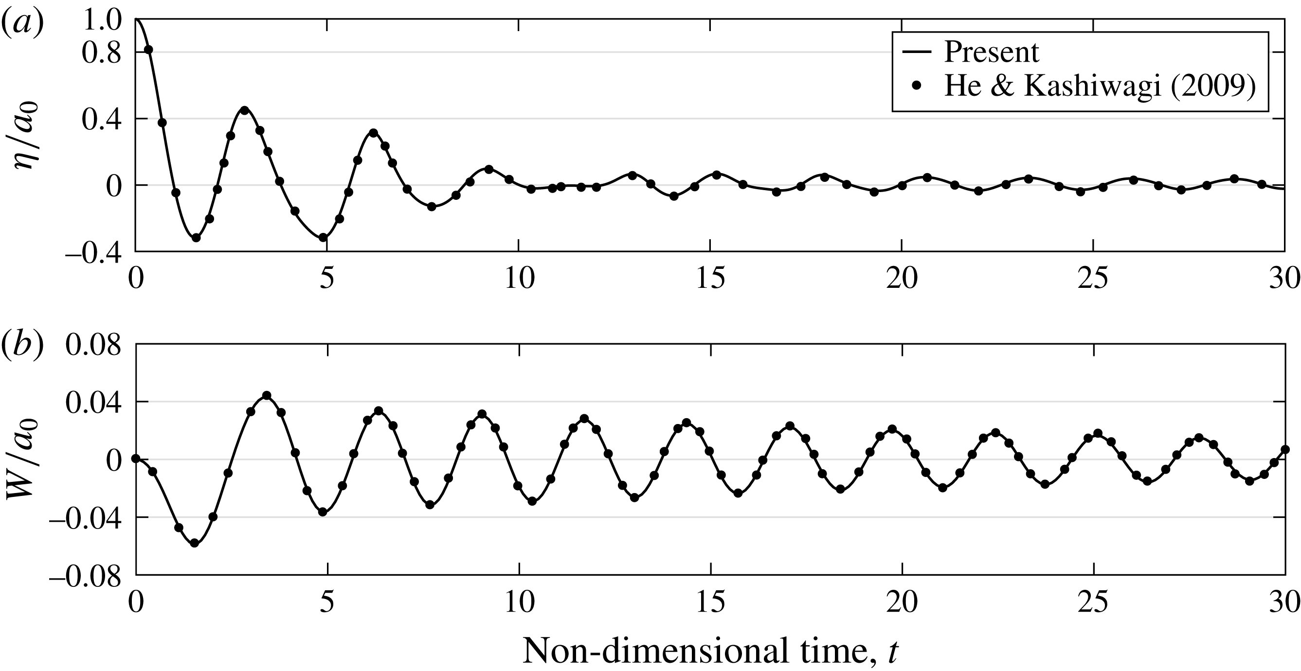
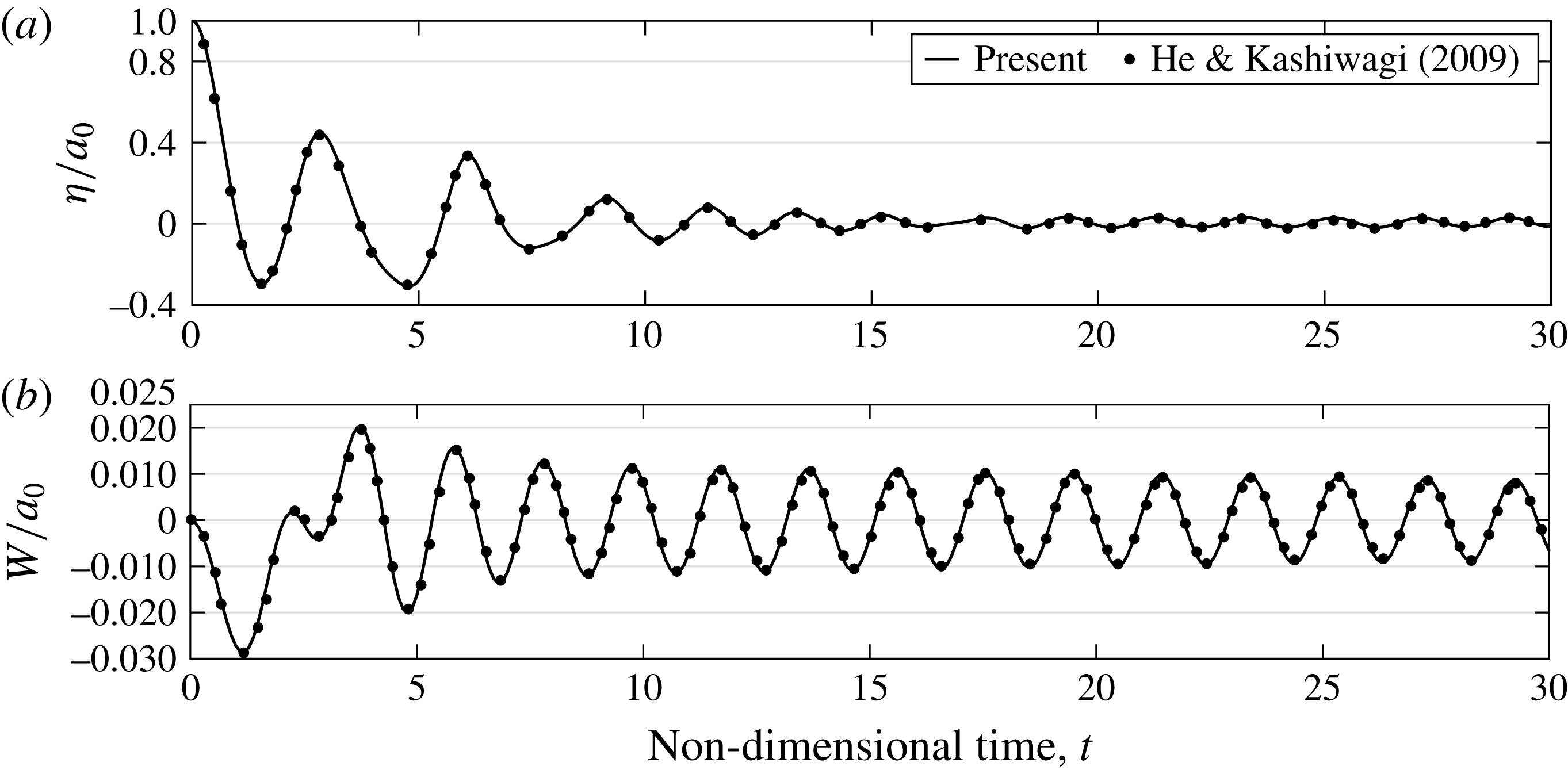
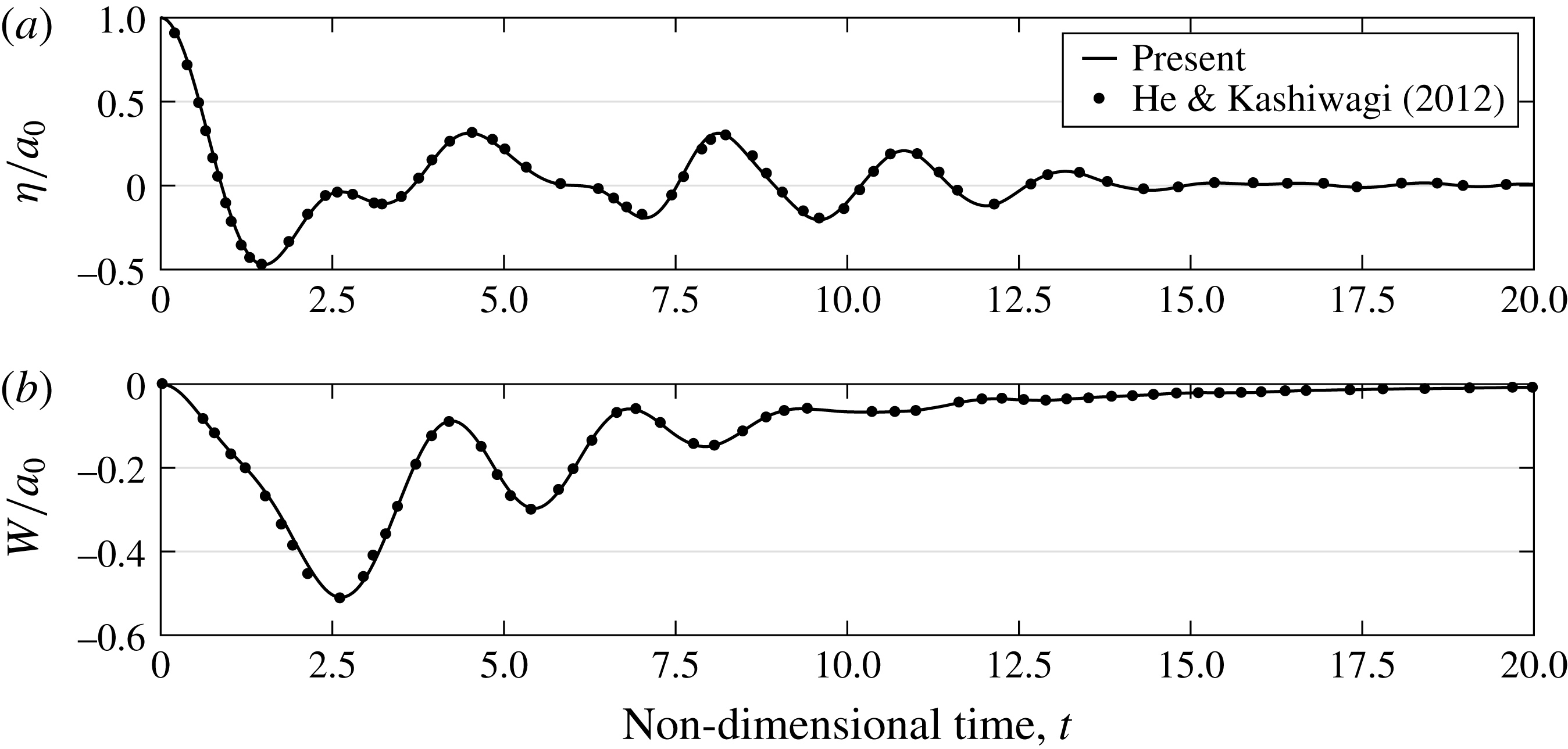
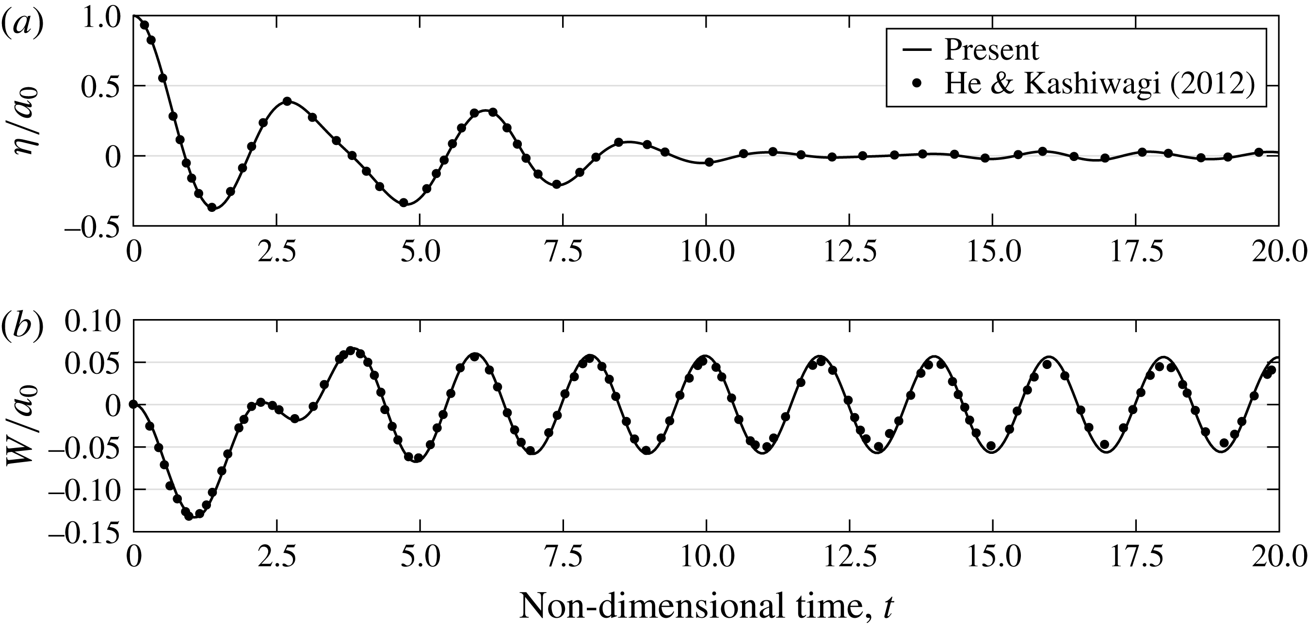
The proposed method for the interaction with a rigid wall supported by springs is verified by comparing its results to an independent set of numerical results presented by He & Kashiwagi (Reference He and Kashiwagi2009). The reference results were obtained using the BEM. An initial pulse-type wave condition, which will be used later for the parametric study, is considered for the verification study. This initial condition is expressed as follows:
 $$\begin{eqnarray}\displaystyle \unicode[STIX]{x1D702}_{0}(x)=\left\{\begin{array}{@{}l@{}}(a_{0}/2)[1+\cos (\unicode[STIX]{x03C0}(x-x_{0})/d)],\quad |x-x_{0}|\leqslant d,\\[4.0pt] 0,\quad |x-x_{0}|>d,\end{array}\right. & & \displaystyle\end{eqnarray}$$
where
 $d$
controls the pulse width,
 $x_{0}$
controls the location of the pulse peak and
 $a_{0}$
is the peak amplitude. Two cases are considered for the verification. In both cases, the pulse width, location and amplitude are selected as
 $d=0.5$
,
 $x_{0}=L-0.7$
and
 $a_{0}=0.1$
. In the first case, the structural parameters are chosen to be
 $m_{s}=1.5$
and
 $k_{s}=10$
, whereas the parameters selected for the second case are
 $m_{s}=1.5$
and
 $k_{s}=20$
. The results of these two cases are shown in figures 3 and 4. In both figures, good agreement appears between the results of the present spectral method and the results of He & Kashiwagi (Reference He and Kashiwagi2009).
Comparison between the results of the present spectral method and those of He & Kashiwagi (Reference He and Kashiwagi2009): (a) normalized time-dependent surface elevation,
 $\unicode[STIX]{x1D702}/a_{0}$
, at
 $x_{0}=L-0.7$
; (b) normalized time-dependent wall vibration,
 $W/a_{0}$
. The parameters used in this example are
 $m_{s}=1.5$
,
 $k_{s}=10$
and
 $a_{0}=0.1$
.

Comparison between the results of the present spectral method and those of He & Kashiwagi (Reference He and Kashiwagi2009): (a) normalized time-dependent surface elevation,
 $\unicode[STIX]{x1D702}/a_{0}$
, at
 $x_{0}=L-0.7$
; (b) normalized time-dependent wall vibration,
 $W/a_{0}$
. The parameters used in this example are
 $m_{s}=1.5$
,
 $k_{s}=20$
and
 $a_{0}=0.1$
.

3.2 Hydroelasticity causing relaxation and amplification
Intuitively, hydroelastic effects are expected to result in relaxation of the hydrodynamic values due to the structural elastic response. Indeed, this intuition has been verified in several works (e.g. Malenica et al.
Reference Malenica, Korobkin, Scolan, Gueret, Delafosse, Gazzola, Mravak, Chen and Zalar2006; He & Kashiwagi Reference He and Kashiwagi2012) by analysing the effect of the structural stiffness on the hydrodynamic results. However, recently Lugni et al. (Reference Lugni, Bardazzi, Faltinsen and Graziani2014) experimentally showed that the opposite effect may occur. Lugni et al. (Reference Lugni, Bardazzi, Faltinsen and Graziani2014) demonstrated that the impact of a ‘flip-through’ event (a term that refers to a specific near-breaking wave impact, see e.g. Cooker & Peregrine Reference Cooker and Peregrine1990, Reference Cooker and Peregrine1992) can be much more significant on a flexible plate than on a rigid one. This suggests that hydroelastic effects may also result in amplification of the hydrodynamic values in the vicinity of the reflecting structure. These two opposite results (i.e. relaxation or amplification of hydrodynamic values) emphasize the need to gain more insight into the effect of structural dynamics on the fluid’s motion and pressure. To this end, the present spectral method is used to compute the maximum wave run-up and wave force on the spring-supported rigid wall for a wide range of wall eigenfrequencies. This is performed for two different initial pulse-type wave conditions. Both of the initial conditions are defined by (3.1) with
 $a_{0}=0.15$
. The first initial condition is referred to as ‘low impulse’ and it is generated with the following parameters:
 $d=2.0$
and
 $x_{0}=L-2.2$
. The second is generated with
 $d=0.5$
and
 $x_{0}=L-0.7$
and is referred to as ‘high impulse’. Finally, in order to examine nonlinear effects, the linear results of the described simulations are plotted as well by simply disregarding the nonlinear terms in (2.22) and (2.32).
Before discussing the results, it will be helpful to determine the peak wave frequency that is generated due to the initial pulse. Using linear theory and assuming an infinite domain, the time-dependent water elevation at
 $x_{0}$
due to the initial pulse (3.1) can be written as
 $$\begin{eqnarray}\displaystyle \unicode[STIX]{x1D702}(x_{0},t)=\frac{ad}{\unicode[STIX]{x03C0}}\int _{0}^{\infty }\hat{\unicode[STIX]{x1D702}}\cos \unicode[STIX]{x1D714}t\,\text{d}k, & & \displaystyle\end{eqnarray}$$
where
 $\unicode[STIX]{x1D714}=\sqrt{k\tanh k}$
according to the linear dispersion relation, and
 $\hat{\unicode[STIX]{x1D702}}$
is defined as
 $$\begin{eqnarray}\displaystyle \hat{\unicode[STIX]{x1D702}}=\left\{\begin{array}{@{}ll@{}}{\displaystyle \frac{\sin kd}{kd\left[1-\left({\displaystyle \frac{k}{\unicode[STIX]{x03C0}/d}}\right)^{2}\right]}}, & k\neq 0\quad \text{or}~\unicode[STIX]{x03C0}/d,\\ 1, & k=0,\\ 1/2, & k=\unicode[STIX]{x03C0}/d.\end{array}\right. & & \displaystyle\end{eqnarray}$$
This solution can be integrated numerically over
 $k$
and subsequently transformed into the frequency domain. Through this procedure, it is found that the peak angular frequency and the corresponding wavenumber which are generated in the low-impulse case are approximately
 $\unicode[STIX]{x1D714}_{0}\cong 0.94$
and
 $k_{0}\cong 1.10$
, respectively. For the high-impulse case the peak angular frequency and the corresponding wavenumber are approximately
 $\unicode[STIX]{x1D714}_{0}\cong 2.04$
and
 $k_{0}\cong 4.17$
. These results imply that the low impulse generates waves that can be characterized as waves in intermediate water depth, whereas the waves generated by the high impulse can be characterized as waves in deep water.
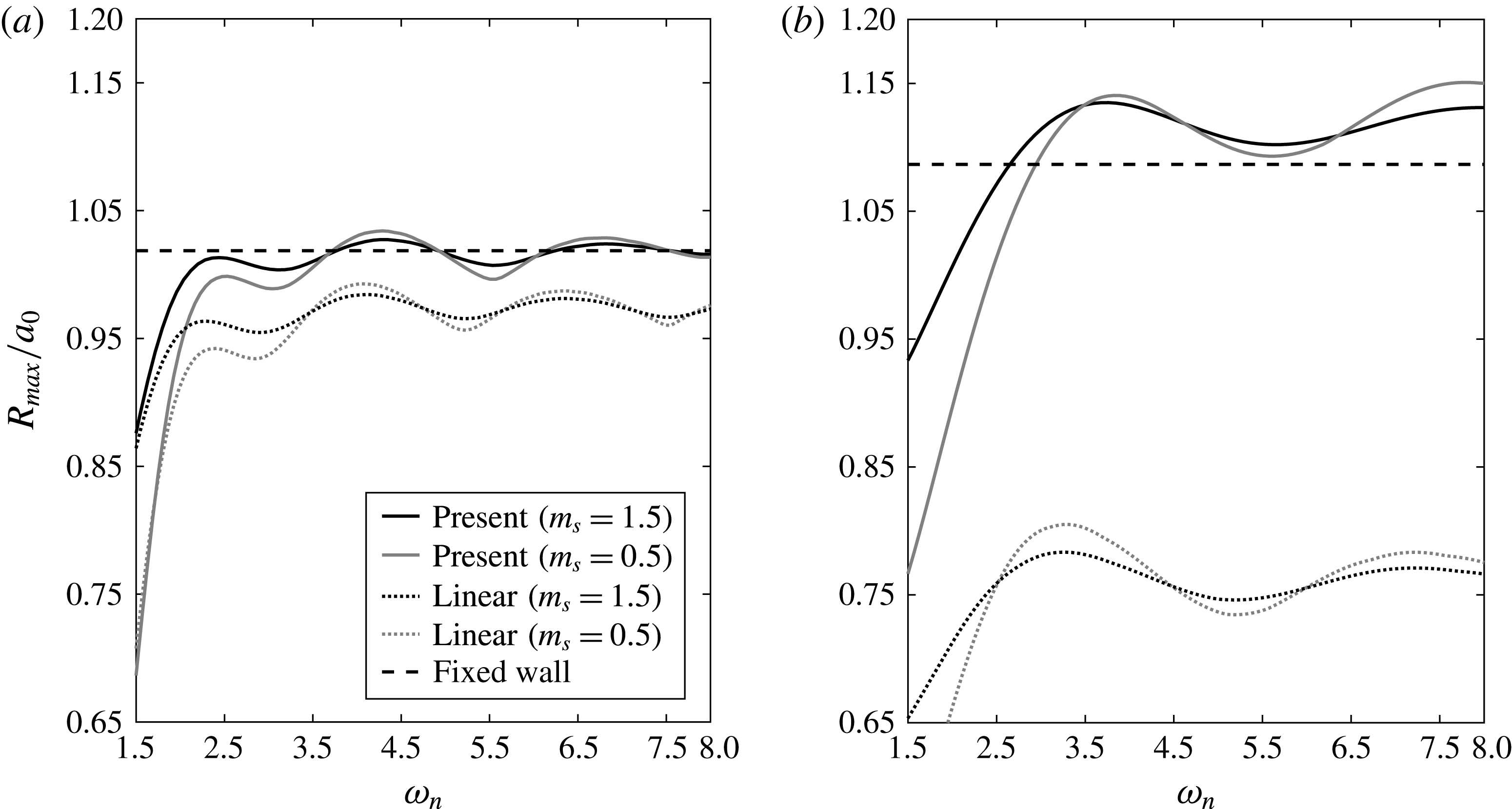
Maximum wave run-up
 $R_{max}$
(normalized by
 $a_{0}$
) versus the eigenfrequency of the wall
 $\unicode[STIX]{x1D714}_{n}$
: (a) low-impulse initial conditions; (b) high-impulse initial conditions.

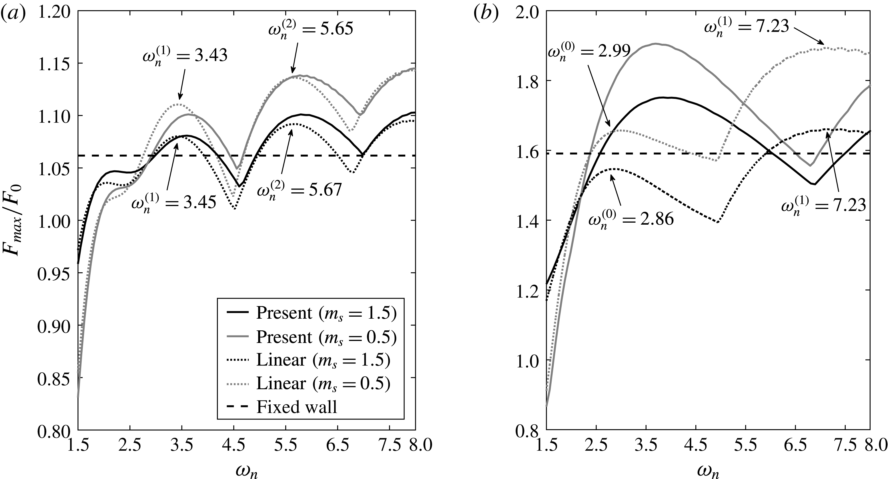
The linear and nonlinear results of the maximum wave run-up
 $R_{max}$
and wave force
 $F_{max}$
on the wall versus the eigenfrequency of the wall,
 $\unicode[STIX]{x1D714}_{n}$
, in the range of
 $1.5\leqslant \unicode[STIX]{x1D714}_{n}\leqslant 8$
, are shown in figures 5 and 6 for both initial wave conditions and for two mass values,
 $m_{s}=0.5$
and
 $m_{s}=1.5$
. The eigenfrequency of the wall is defined as follows:
 $$\begin{eqnarray}\displaystyle \unicode[STIX]{x1D714}_{n}=\sqrt{k_{s}/(m_{s}+\tilde{\unicode[STIX]{x1D6FF}})}, & & \displaystyle\end{eqnarray}$$
where
 $\tilde{\unicode[STIX]{x1D6FF}}$
is the linear added-mass term defined according to the linear conditions on the free water surface, and therefore, as opposed to the definition in (2.33), can be evaluated in advance using the following expression (see e.g. Billingham & King Reference Billingham and King2000):
 $$\begin{eqnarray}\displaystyle \tilde{\unicode[STIX]{x1D6FF}}=\mathop{\sum }_{q}{\displaystyle \frac{2\sin ^{2}k_{e}(q)}{k_{e}^{2}(q)[k_{e}(q)+{\textstyle \frac{1}{2}}\sin 2k_{e}(q)]}}. & & \displaystyle\end{eqnarray}$$
The wavenumbers,
 $k_{e}(q)$
, are the solutions of
 $\unicode[STIX]{x1D714}_{n}^{2}=-k_{e}\tan k_{e}$
. Therefore, the linear added mass depends on
 $\unicode[STIX]{x1D714}_{n}$
through
 $k_{e}(q)$
. The solution for
 $\unicode[STIX]{x1D714}_{n}$
,
 $\tilde{\unicode[STIX]{x1D6FF}}$
and
 $k_{e}(q)$
is obtained iteratively using (3.4) and (3.5), and the relation between
 $\unicode[STIX]{x1D714}_{n}$
and
 $k_{e}(q)$
.
Maximum wave force
 $F_{max}$
(normalized by
 $F_{0}$
) versus the eigenfrequency of the wall
 $\unicode[STIX]{x1D714}_{n}$
: (a) low-impulse initial conditions; (b) high-impulse initial conditions.

Finally, note that the maximum run-up is normalized by the initial wave amplitude,
 $a_{0}$
, and the maximum wave force is normalized by the reference wave force,
 $F_{0}$
. The reference wave force is defined as the linear dynamic force obtained under a crest of a uniform wave train. Therefore,
 $F_{0}$
can be calculated by integrating the linear wave dynamic pressure as follows:
 $$\begin{eqnarray}\displaystyle F_{0}=\int _{-1}^{0}a_{0}{\displaystyle \frac{\cosh [k_{0}(z+1)]}{\cosh k_{0}}}\,\text{d}z=a_{0}{\displaystyle \frac{\tanh k_{0}}{k_{0}}}, & & \displaystyle\end{eqnarray}$$
where
 $a_{0}$
is the initial pulse amplitude and
 $k_{0}$
is the wavenumber that corresponds to the peak angular frequency.
Both the linear and the nonlinear results of the wave maximum run-up and wave force reveal an interesting phenomenon. The values demonstrate a prominent fluctuation around the hydrodynamic values obtained in the case of a fixed wall (which is calculated by setting
 $\unicode[STIX]{x1D719}_{vw}=0$
; see also the formulation in Akrish et al. (Reference Akrish, Schwartz, Rabinovitch and Agnon2016b
)) as a function of
 $\unicode[STIX]{x1D714}_{n}$
. For lower values of
 $\unicode[STIX]{x1D714}_{n}$
, relaxation of the hydrodynamic values is observed. Comparing the high- and low-impulse results, the fluctuation frequency is higher for the low-impulse case. The reason for that is discussed below. In addition, the maximum wave force values are also higher in the low-impulse case, as the vertical distribution of wave pressure reduces more slowly for longer waves. This observation cannot be detected directly from the figures, but by realising that the value of
 $F_{0}$
for the low-impulse case is approximately three times higher than for the high-impulse case. On the other hand, the maximum run-up values are higher in the high-impulse case. This is because the nonlinear contributions in the high-impulse case are more significant as a result of higher water surface steepness. The significance of nonlinear contributions in the high-impulse case versus the low-impulse case is also reflected by comparing the nonlinear results with the linear ones in figures 5 and 6.
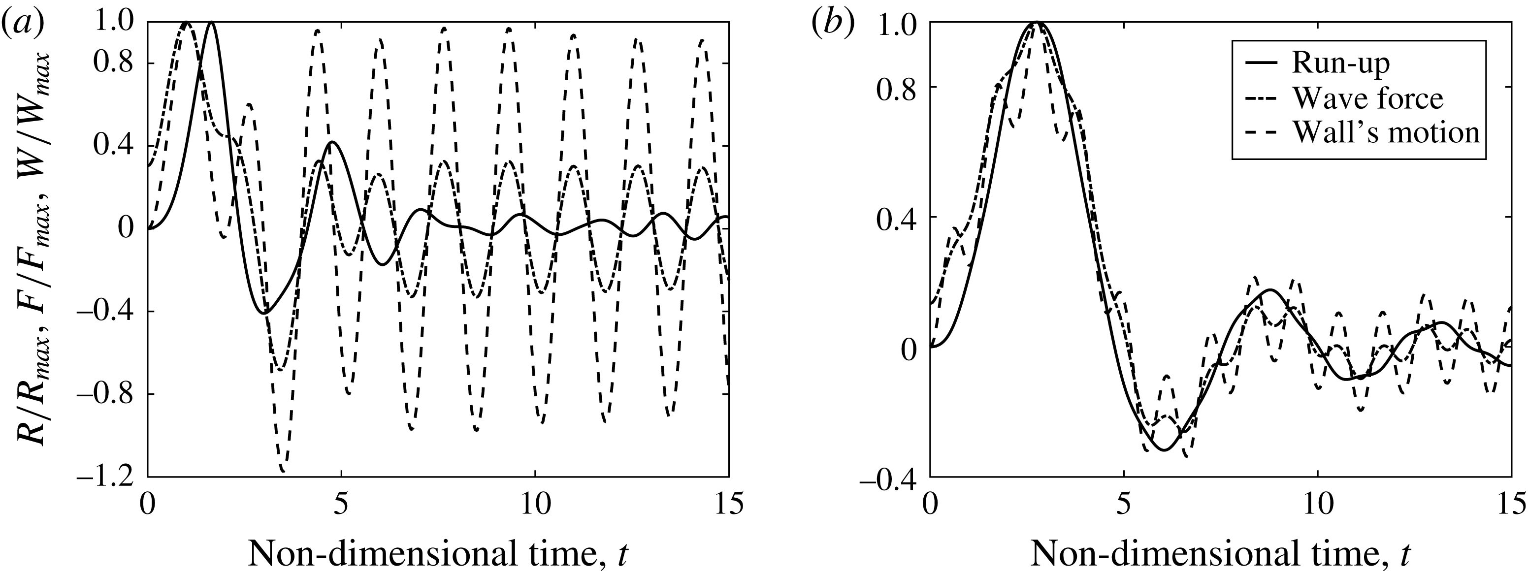
The mechanism that leads to the fluctuation phenomenon of the maximum wave run-up and wave force values is examined by looking at two sets of results. The first concerns the extreme run-up value which is obtained for the high-impulse case with
 $\unicode[STIX]{x1D714}_{n}\cong 3.78$
and
 $m_{s}=1.5$
(note that in this layout an extreme wave force value is obtained as well), while the second concerns the extreme wave force value which occurs for the low-impulse case with
 $\unicode[STIX]{x1D714}_{n}\cong 5.65$
and
 $m_{s}=1.5$
. The mechanism leading to these extreme interaction events is explained in figure 7, which compares the time-dependent results of the run-up and wave force with the wall displacement for each of these cases. As can be deduced from figure 7(a), extreme run-up value occurs in the first case due to a constructive interference between the wave run-up and the wall’s negative velocity. In addition, similar interference is detected between the wave force and the wall’s negative acceleration. This is a special case in which the two phases interfere constructively. This situation may only occur when the moment of maximum wave force does not overlap with the moment of maximum run-up. In the second case, the incoming wave has lower steepness, leading to a shared moment of maximum wave run-up and wave force. Thus, in this case, the previous special situation is not possible, and only the wave force and the wall’s negative acceleration interfere constructively (see figure 7
b). This leads to the extreme wave force event which appears in figure 6. Following this analysis, it can also be deduced that the lower points of maximum wave run-up and wave force (the values’ relaxation points) in figures 5 and 6 occur when the corresponding phases of the wall and the fluid motion interfere destructively.
Time-dependent comparison between the run-up
 $R$
, the wave force
 $F$
and the wall displacement
 $W$
for two extreme interaction examples: (a) high-impulse initial conditions with
 $\unicode[STIX]{x1D714}_{n}\cong 3.78$
and
 $m_{s}=1.5$
; (b) low-impulse initial conditions with
 $\unicode[STIX]{x1D714}_{n}\cong 5.65$
and
 $m_{s}=1.5$
.

This analysis calls for a more general picture that can describe the hydrodynamic response due to the considered wave impulses for any choice of
 $m_{s}$
. As a first step towards this goal, the linear problem is examined in greater detail. First, the possibility of constructing a general curve of the maximum wave force against
 $\unicode[STIX]{x1D714}_{n}$
is examined. To this end, a general condition to obtain an extremum can be formulated. As implied in figure 7(b), and in accordance with the initial conditions of the wall (
 $W=0,W_{t}=0$
), an extremum is obtained when the ratio between the time of maximum wave force,
 $T_{0}$
, and the period of the wall’s oscillations,
 $2\unicode[STIX]{x03C0}/\unicode[STIX]{x1D714}_{n}$
, equals
 $j+1/2$
. Namely, the values,
 $\unicode[STIX]{x1D714}_{n}^{(j)}$
, where extrema are expected to form may be predicted by the following expression:
 $$\begin{eqnarray}\displaystyle \unicode[STIX]{x1D714}_{n}^{(j)}=2\unicode[STIX]{x03C0}(j+1/2)/T_{0},\quad j=0,1,2,\ldots . & & \displaystyle\end{eqnarray}$$
Under this condition, the wall’s negative acceleration is expected to interfere constructively with the maximum incoming waves force. Note that (3.7) also explains the higher fluctuation frequency in the low-impulse case, as for this loading case the value of
 $T_{0}$
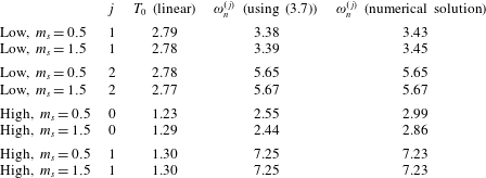
is larger. In order to check the prediction of (3.7), eight values of
 $\unicode[STIX]{x1D714}_{n}^{(j)}$
, which are indicated in figure 6, are examined in table 1. The table summarizes the extremum number,
 $j$
, the associated
 $T_{0}$
and the values for
 $\unicode[STIX]{x1D714}_{n}^{(j)}$
as predicted by (3.7) and by figure 6 for the two considered masses and wave conditions (low or high refers to low impulse or high impulse).
Sampled values of
 $T_{0}$
and
 $\unicode[STIX]{x1D714}_{n}$
, associated with extrema of maximum wave force on the wall supported by springs.

The following observations can be readily deduced from the values in table 1. First, it is clear that
 $T_{0}$
is a function of both
 $\unicode[STIX]{x1D714}_{n}$
and
 $m_{s}$
. Secondly, even if the influence of
 $m_{s}$
on the value of
 $T_{0}$
is taken into account (as done for the calculated values of
 $\unicode[STIX]{x1D714}_{n}^{(j)}$
using (3.7)), there are still discrepancies between the values of
 $\unicode[STIX]{x1D714}_{n}^{(j)}$
as predicted by (3.7) and numerically, and between the values of
 $\unicode[STIX]{x1D714}_{n}^{(j)}$
for different
 $m_{s}$
. The reason for that is directly related to the decay rate of the oscillating wall, which is a function of the two parameters,
 $\unicode[STIX]{x1D714}_{n}$
and
 $m_{s}$
, as well. Note that stronger decay rate will occur for lower values of
 $\unicode[STIX]{x1D714}_{n}$
and
 $m_{s}$
(when the oscillations of the wall radiate longer waves). Therefore, for lower values of
 $\unicode[STIX]{x1D714}_{n}$
, the positions
 $\unicode[STIX]{x1D714}_{n}^{(j)}$
tend to be higher when considering lower values of
 $m_{s}$
. Following these observations, it may concluded that, in order to construct a general curve for the maximum wave force for any value of
 $m_{s}$
, one has to formulate a different independent variable which, as opposed to
 $\unicode[STIX]{x1D714}_{n}$
, accounts for the effect of
 $m_{s}$
on
 $T_{0}$
and on the decay rate. Further complexity is introduced when formulating the normalized dependent variable on the vertical axis, for which the effect of the decay rate and its dependence on
 $m_{s}$
also hampers the construction of a general curve for any value of
 $m_{s}$
.
The generalization of the nonlinear problem is expected to be much more challenging, as in this case both the added mass and the decay rate are functions of the high-order contributions of the hydrodynamic value, which in turn depend on
 $m_{s}$
. The influence of nonlinearity on the values of
 $\unicode[STIX]{x1D714}_{n}^{(j)}$
is clearly evident for the high-impulse case, as shown in figure 6(b). Note that the lower frequency in the fluctuation of the nonlinear curve in figure 6(b) is also a result of a much shorter
 $T_{0}$
caused by the effect of the nonlinear contributions.
Following the discussion above, it was decided to concentrate on the main goals of this study through a couple of representative examples. The challenging task of generalizing the results that are shown here for any value of
 $m_{s}$
should be preserved for a separate study. Nevertheless, note that, for the linear case, (3.7) provides a good approximation, especially for higher values of
 $\unicode[STIX]{x1D714}_{n}^{(j)}$
, where hydroelastic effects become weak.
This section is closed by noting that the present analysis demonstrates the hydroelastic effects only in a qualitative manner. As a result it tends to somewhat underestimate the amplification reflected by the maximum results that correspond to the elastic and the rigid walls. Quantitatively, Lugni et al. (Reference Lugni, Bardazzi, Faltinsen and Graziani2014) showed that the impact pressure of a flip-through event can be twice as high due to the hydroelastic effects.
4 Hydroelastic interaction of a deformable wall and an incident wave group
In this section, the hydroelastic interaction of the general continuous case of an elastic deformable wall and an incident water wave group is considered. The generation of the wave group is simulated by means of a piston wavemaker at the entrance of the numerical flume (see figure 1). This problem of interaction can be considered as a composition of two stages: the group evolution stage, in which the group evolves along the flume until it meets the wall, and the reflection stage, during which the group–wall interaction occurs. The main goal of the investigation is to analyse the role of nonlinearity during both of these stages and to analyse the role of hydroelasticity during the reflection stage. As has been done in § 3, the method is verified before presenting the main investigation.
4.1 Verification of the method for the interaction with the deformable wall case
The proposed method for the interaction with the deformable wall is verified using the results presented in He & Kashiwagi (Reference He and Kashiwagi2012). These results were derived using a numerical code which is based on the BEM for solving the fluid motion and on the FEM for the solution of the wall motion. The verification considers two cases. The first one concerns the hydroelastic interaction of an incoming wave field and a wall with fixed–free boundary conditions, see (2.9). The second case deals with the same problem of interaction, but with fixed–fixed boundary conditions, see (2.10). For both cases, the motion is triggered by the pulse-type wave, equation (3.1), that was introduced in § 3, with initial parameters that correspond to the high-impulse case and with an initial wave amplitude of
 $a_{0}=0.01$
. The structural parameters are
 $k_{s}=0.01$
,
 $m_{s}=0.1$
and
 $\unicode[STIX]{x1D6E4}=0$
. Note that the value selected for
 $\unicode[STIX]{x1D6E4}$
violates the assumption that the run-up on the wall is lower than the wall’s height; however, due to the low value of the initial wave amplitude, this violation will result in a negligible effect. The results of these examples appear in figures 8 and 9 and show that both the surface elevation and the motion of the wall, which were obtained using the present spectral method, are in good agreement with the results of He & Kashiwagi (Reference He and Kashiwagi2012). A small deviation, which is attributed to the decay rate, appears in the fixed–fixed wall vibration in figure 9(b). Yet this discrepancy, which is not observed in the surface elevation versus time curve, is not significant and it may be an outcome of artificial damping in the reference model. The satisfying verification results allow us to return the focus on the main investigation of this section.
Comparison between the results of the present spectral method and those of He & Kashiwagi (Reference He and Kashiwagi2012) for the fixed–free case: (a) normalized time-dependent surface elevation,
 $\unicode[STIX]{x1D702}/a_{0}$
, at
 $x_{0}=L-0.7$
; (b) normalized time-dependent horizontal displacement at the centre of the wall,
 $W/a_{0}$
. The parameters used in this example are
 $k_{s}=0.01$
,
 $m_{s}=0.1$
and
 $a_{0}=0.01$
.

Comparison between the results of the present spectral method and those of He & Kashiwagi (Reference He and Kashiwagi2012) for the fixed–fixed case: (a) normalized time-dependent surface elevation,
 $\unicode[STIX]{x1D702}/a_{0}$
, at
 $x_{0}=L-0.7$
; (b) normalized time-dependent horizontal displacement at the centre of the wall,
 $W/a_{0}$
. The parameters used in this example are
 $k_{s}=0.01$
,
 $m_{s}=0.1$
and
 $a_{0}=0.01$
.

4.2 The role of nonlinearity and hydroelasticity
The main investigation concerns the interaction of the deformable wall with an incident wave group. The considered wave group is generated by the motion of the piston wavemaker with the following stroke function:
 $$\begin{eqnarray}\displaystyle S(t)=S_{0}\exp \left(-\left(\frac{t-\unicode[STIX]{x1D70F}}{\unicode[STIX]{x1D707}T_{0}}\right)^{2}\right)\cos (\unicode[STIX]{x1D714}_{0}(t-\unicode[STIX]{x1D70F})),\quad \text{on}~x=0. & & \displaystyle\end{eqnarray}$$
This function generates a periodic wave modulated by a Gaussian envelope, where
 $\unicode[STIX]{x1D707}$
controls the envelope width, and
 $\unicode[STIX]{x1D714}_{0}$
is the carrier wave angular frequency, which is defined by the carrier wave period
 $T_{0}=2\unicode[STIX]{x03C0}/\unicode[STIX]{x1D714}_{0}$
and associated with the carrier wavenumber
 $k_{0}$
through the linear dispersion relation (
 $\unicode[STIX]{x1D714}_{0}=\sqrt{k_{0}\tanh k_{0}}$
). The highest stroke amplitude,
 $S_{0}$
, relates to the maximum wave amplitude,
 $a_{0}$
, through the wavemaker’s amplitude-to-stroke ratio (Dean & Dalrymple Reference Dean and Dalrymple1991). Finally,
 $\unicode[STIX]{x1D70F}$
controls the initiation of the wavemaker motion so as to avoid abrupt wavemaker motion, which may result in unstable evolution. In the present investigation, the incident wave group is generated using the following values:
 $a_{0}=0.03$
,
 $\unicode[STIX]{x1D714}_{0}=2.12$
(
 $k_{0}=4.5$
),
 $\unicode[STIX]{x1D707}=5$
and
 $\unicode[STIX]{x1D70F}=12$
. The interaction between the wave group and the deformable wall is studied for a wide range of flexural stiffness:
 $0.5\leqslant k_{s}\leqslant 6$
. In addition, the considered boundary conditions of the wall obey the definition of the fixed–free boundaries given in (2.9). The remaining structural parameters are:
 $m_{s}=0.25$
and
 $\unicode[STIX]{x1D6E4}=0.1$
.
As mentioned above, the goal of the investigation is to analyse the roles of nonlinearity and hydroelasticity throughout the evolution stage and the reflection stage. The role of nonlinearity is examined through comparison with the linear results, which are obtained by neglecting the nonlinear terms in (2.22) and (2.25). The role of hydroelasticity is examined by comparison with the results of an uncoupled analysis, in which the hydrodynamic and the corresponding structural response are solved separately. This analysis assumes a fixed wall for the solution of the fluid motion and pressure (i.e. setting
 $\unicode[STIX]{x1D719}_{vw}=0$
), while the solution of the wall’s response is obtained using a simplified condition on the free water surface in order to evaluate the required added-mass components in (2.28). This simplified free surface condition is based on the high-frequency approximation of the linear free surface condition (i.e.
 $\lim _{\unicode[STIX]{x1D714}\rightarrow \infty }-\unicode[STIX]{x1D714}^{2}\unicode[STIX]{x1D719}+g\unicode[STIX]{x1D719}_{z}=-\unicode[STIX]{x1D714}^{2}\unicode[STIX]{x1D719}=0$
). This approximation has been used in several studies in order to gain insight into the dynamic characteristics of vertical plates in contact with water (see e.g. Zhou & Cheung Reference Zhou and Cheung2000; Ergin & Uğurlu Reference Ergin and Uğurlu2003; Hashemi, Karimi & Taher Reference Hashemi, Karimi and Taher2010). Such analysis provides reasonable results for relatively stiff plates (Fu & Price Reference Fu and Price1987). Using the present spectral method, the evaluation of the added-mass components according to the high-frequency approximation are obtained by solving (2.13) with the additional condition
 $\unicode[STIX]{x1D719}_{vw}=0$
on the free surface and substituting the resulting
 $C_{i,b}$
values into (2.28), for which
 $p_{j}$
and
 $\unicode[STIX]{x1D702}$
are set to zero. The results of the investigation are discussed in the following two parts. The first part considers the maximum absolute values as a function of
 $k_{s}$
. The second part examines three specific simulations, each representing a different scenario of wave–wall interaction. Note that all the results are normalized by reference values. The wave run-up and wall’s displacement values are normalized by
 $a_{0}$
, and the wave force is normalized by
 $F_{0}$
(see the definition in (3.6)).
4.2.1 The interaction results as a function of the flexural stiffness
 $k_{s}$

As a way to gain insight into the dynamic behaviour of the wave–wall system, the wall’s eigenfrequencies are evaluated first. To this end, two approaches are employed, the high-frequency approximation and the linear theory. In the discussion above, the high-frequency approximation is introduced as a method to evaluate the added-mass components. Once the added-mass components are known, the eigenfrequencies are obtained by taking the square root of the eigenvalues of
 $\unicode[STIX]{x1D614}_{eff}^{-1}\unicode[STIX]{x1D612}_{eff}$
(see (2.25)). This procedure also holds when considering the linear theory. But, as opposed to the high-frequency approximation, the linear theory preserves the complete linear condition on the free water surface. As a result, the added-mass components depend on the frequencies of the incoming waves. In this approach, the added-mass components are calculated using the expression
 $$\begin{eqnarray}\displaystyle & \displaystyle \tilde{\unicode[STIX]{x1D6FF}}_{ij}=\mathop{\sum }_{q}\tilde{C}_{j,q}\int _{-1}^{0}f_{i}\cos [k_{e}(q)(z+1)]\,\text{d}z, & \displaystyle\end{eqnarray}$$
which assumes that the wall interacts with a uniform wave train characterized by
 $\unicode[STIX]{x1D714}$
, where, as mentioned in § 3,
 $k_{e}(q)$
is the
 $q$
solution of
 $\unicode[STIX]{x1D714}^{2}=-k_{e}\tan k_{e}$
, and
 $\tilde{C}_{j,q}$
is defined as
 $$\begin{eqnarray}\displaystyle & \displaystyle \tilde{C}_{j,q}=\frac{\displaystyle \int _{-1}^{0}f_{j}\cos [k_{e}(q)(z+1)]\,\text{d}z}{\displaystyle k_{e}(q)\tanh [k_{e}(q)L]\int _{-1}^{0}\cos ^{2}[k_{e}(q)(z+1)]\,\text{d}z}. & \displaystyle\end{eqnarray}$$
This expression generalizes a similar expression for the case of a rigid wall supported by springs (see (3.5)) derived, for example, in Billingham & King (Reference Billingham and King2000). Note that (4.2) introduces further approximation by the assumption that the wall interacts with a uniform wave train. Therefore, by using the carrier frequency of the incident wave group,
 $\unicode[STIX]{x1D714}_{0}$
, (4.2) serves as an approximation to the linear approach.
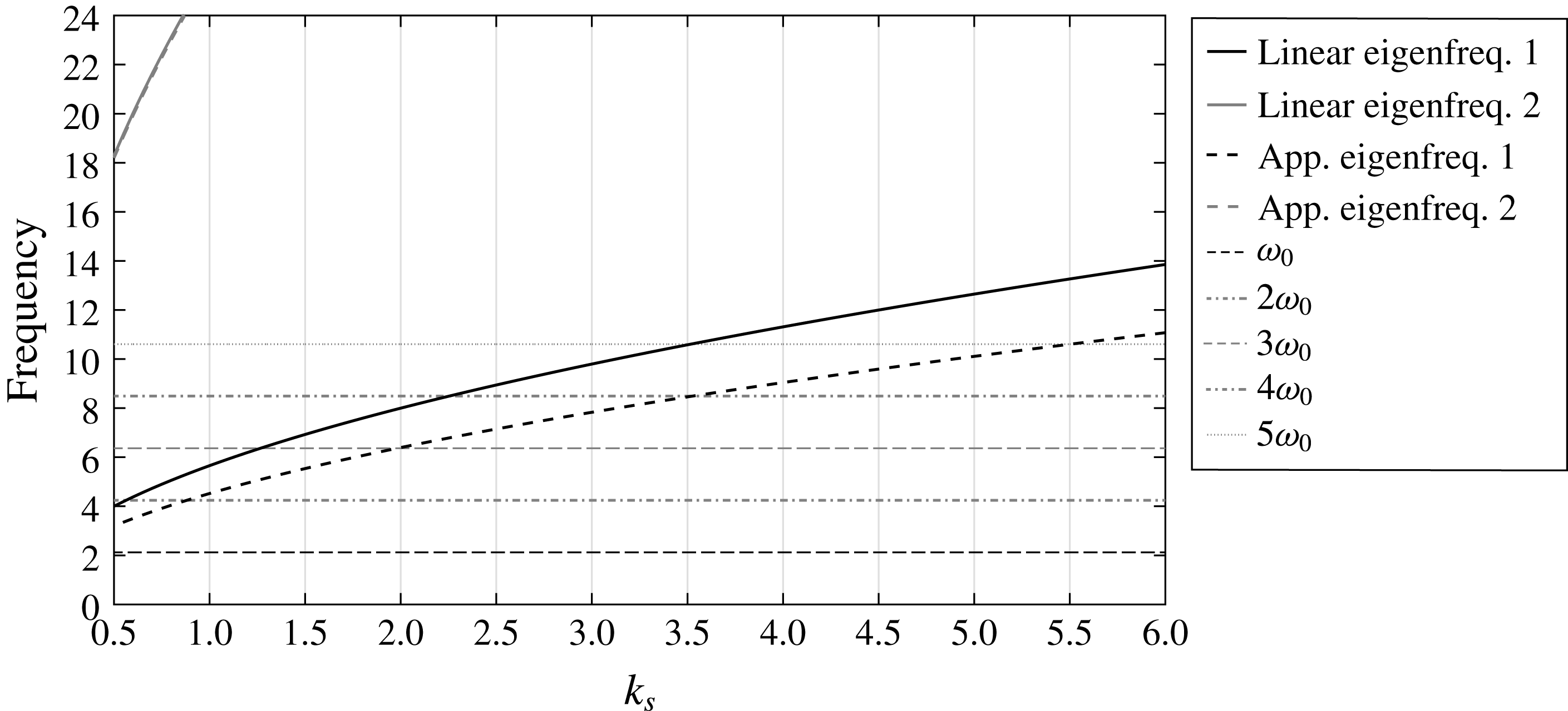
The eigenfrequencies of the first and second modes of the wall versus
 $k_{s}$
, evaluated through the linear theory (solid line) (using
 $\unicode[STIX]{x1D714}=\unicode[STIX]{x1D714}_{0}$
as the representative frequency) and the high-frequency approximation (dashed line) (
 $\unicode[STIX]{x1D714}\rightarrow \infty$
).

The results of the eigenfrequencies, using both approximations, are plotted as a function of
 $k_{s}$
in figure 10. For reference, several horizontal lines that denote the first- and higher-order carrier frequencies of the incident wave group are also shown in figure 10. The intersections between these horizontal lines and the eigenfrequency curves indicate the regions of
 $k_{s}$
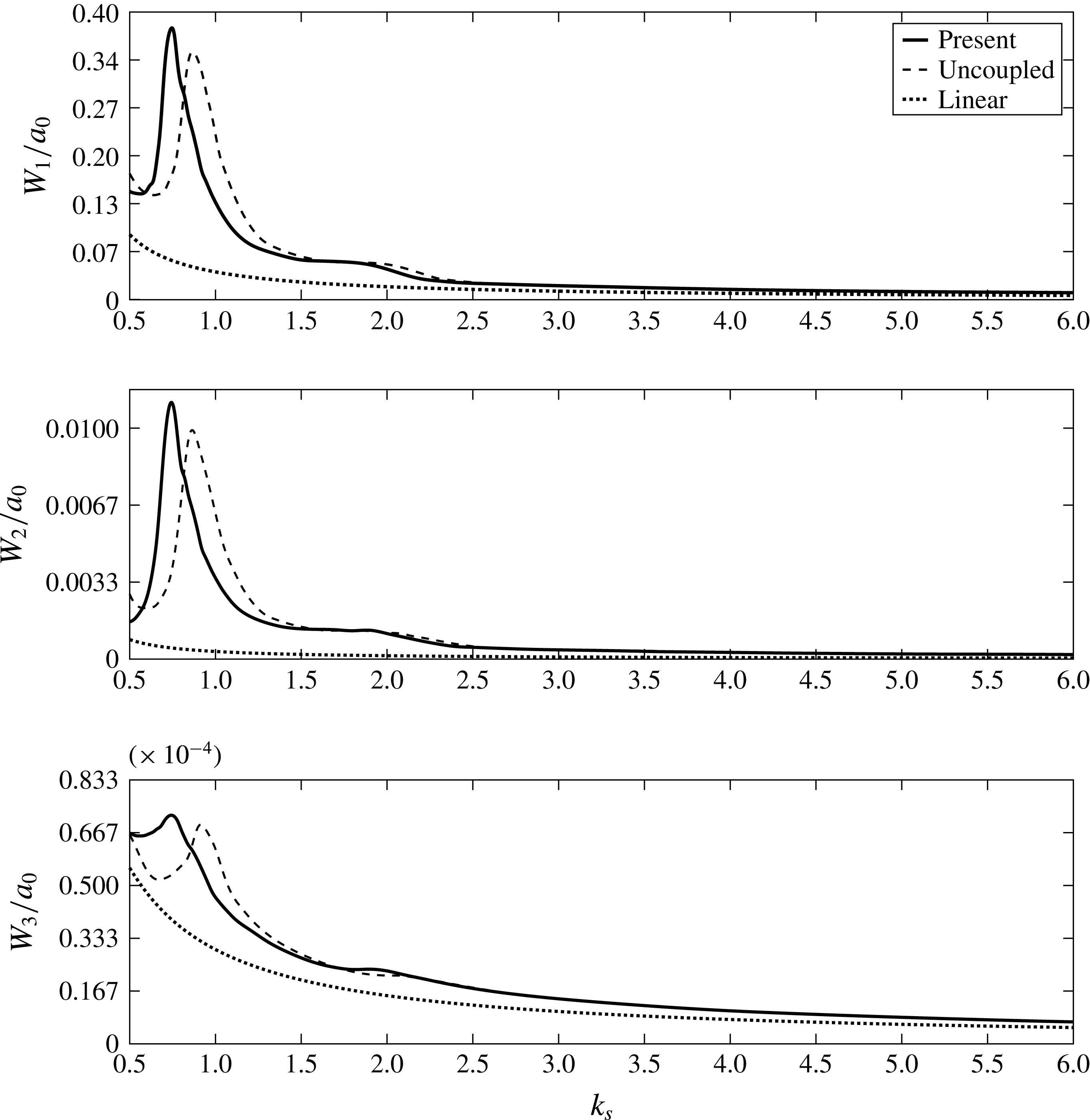
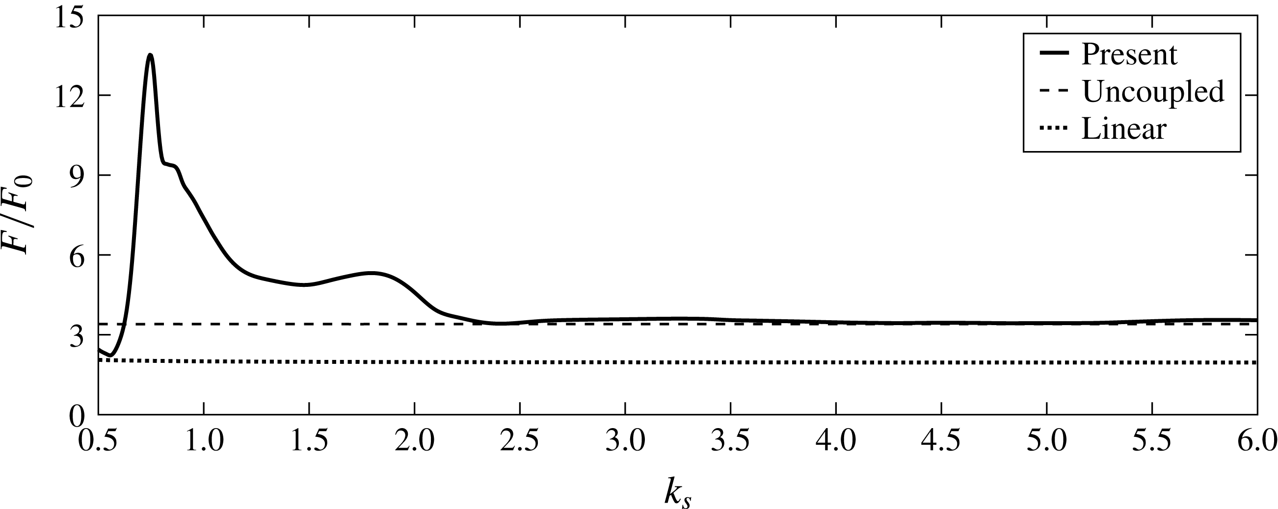
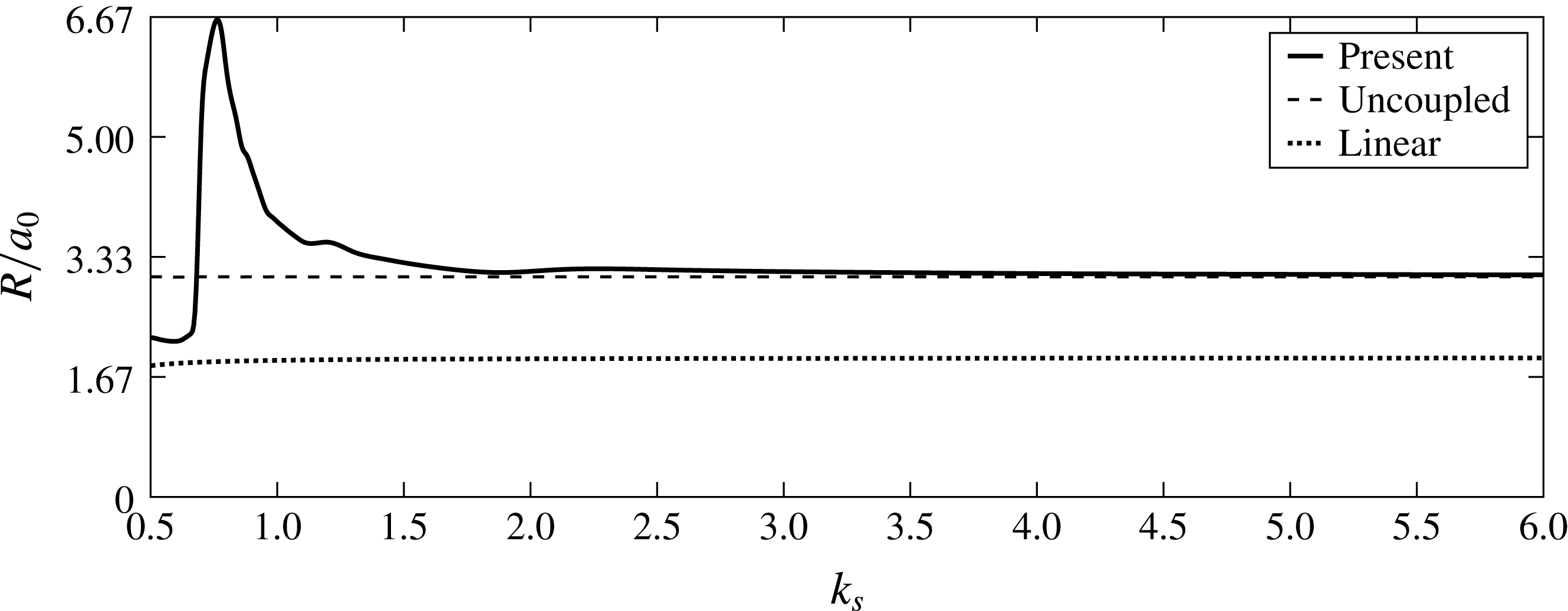
for which resonant interactions are expected. Indeed, figures 11–13, which show the wall’s deflections, the force exerted on the wall and the run-ups, reveal peak values in these regions due to resonant interactions. The occurrence of these resonance scenarios explains the importance of the role of nonlinearity during the evolution stage, through which the higher harmonics are generated. Obviously, the linear results cannot predict such scenarios. Referring again to figure 10, it is clear that only the first eigenfrequency of the wall intersects with the frequencies of the waves.
Maximum absolute displacement of the wall’s first three modes,
 $W_{1}$
,
 $W_{2}$
and
 $W_{3}$
, at the mid-water depth (normalized by
 $a_{0}$
) versus
 $k_{s}$
: comparison between the results of the present spectral method, the uncoupled analysis and the linear analysis.

The question arises as to why the rest of the wall’s modes are in resonance as well, as shown in figure 11. This is because the modes of the wall are coupled through the added-mass terms,
 $\unicode[STIX]{x1D6FF}_{ij}$
. The vibration of one mode creates water pressure, the distribution of which induces the activation of the other modes. Figure 10 also explains why the locations of the resonant interactions, as predicted by the present spectral method, are different from those found with the uncoupled analysis. The reason is that the present method accounts for the coupling between the frequencies of the waves and the wall (as in the linear approximation). This coupling becomes weaker as the frequencies of the incoming waves are higher (and eventually disappears as in the high-frequency approximation). This is why the agreement between the results of the present method and the uncoupled analysis in figure 11 is stronger around the region of
 $k_{s}\cong 1.8$
, where resonant interaction due to wave load of third-order harmonics occurs, as compared to the region of
 $k_{s}\cong 0.8$
, where resonant interaction due to wave load of second-order harmonics takes place. The role of hydroelasticity also results in different maximum displacement values, as appears by comparing the results of the present method and the uncoupled analysis in figure 11. Close to
 $k_{s}\cong 0.5$
, the wall’s response causes relaxation of the wave loads (see figure 12), which in turn leads to lower displacement value. On the other hand, in a region of resonant interaction, the wall’s response amplifies the hydrodynamic pressure (as deduced from figure 12), which in turn leads to higher displacement value. These effects highlight the significance of the role of hydroelasticity in the attempt to describe the interaction of waves and elastic structures.
Maximum absolute force,
 $F$
(normalized by
 $F_{0}$
), exerted by the incident wave group, versus
 $k_{s}$
: comparison between the results of the present spectral method, the uncoupled analysis and the linear analysis.

Maximum absolute run-up,
 $R$
(normalized by
 $a_{0}$
), on the wall induced by the incident wave group, versus
 $k_{s}$
: comparison between the results of the present spectral method, the uncoupled analysis and the linear analysis.

Finally, it is desired to draw attention to the hydrodynamic results. Figure 12 presents the maximum absolute value (normalized by
 $F_{0}$
) of the wave force on the wall as a function of
 $k_{s}$
. The figure shows nicely all the regions where resonant interactions take place. This includes the resonant interactions due to fourth- and fifth-order excitation load, which appear around
 $k_{s}\cong 3.3$
and
 $k_{s}\cong 5.7$
, respectively. The highest peak is obtained around
 $k_{s}\cong 0.8$
, where the second-order harmonics evoke resonant interaction. The results in this region exceed the limits of the simulations as the run-up values depicted in figure 13 exceed
 $\unicode[STIX]{x1D6E4}$
. At the highest peak the run-up reaches close to
 $R\cong 0.2$
(almost seven times the initial group amplitude,
 $a_{0}$
), which is above the height of the wall. The analysis treats the region above the height of the wall as fixed, and therefore could describe those run-up values, but the values in this region should only be taken as an approximation. However, these values do imply that, in certain circumstances, in which hydroelastic and nonlinear effects are significant, the hydrodynamic and structural results can be much more significant than the linear ones.
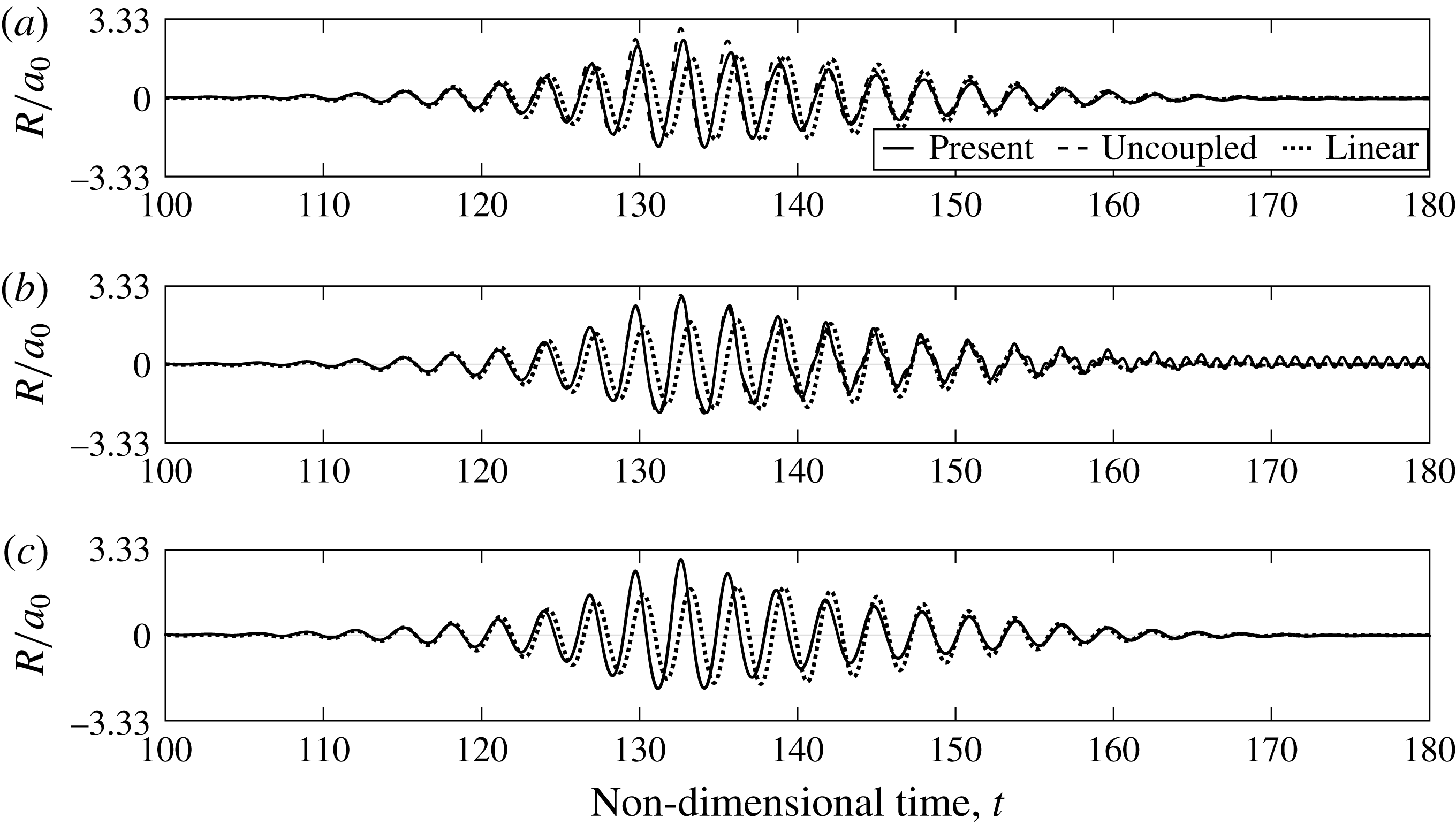
The normalized wave group run-up,
 $R/a_{0}$
, on the wall using the present spectral method, the uncoupled analysis and the linear analysis for the following values of flexural stiffness: (a)
 $k_{s}=0.5$
, (b)
 $k_{s}=1.85$
, (c)
 $k_{s}=3$
.

4.2.2 Analysis of the time-dependent interaction of three interaction scenarios
Following the results of the interaction versus
 $k_{s}$
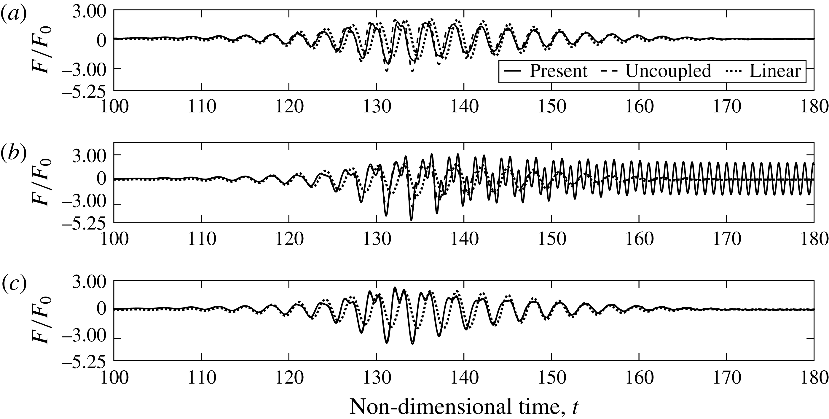
, three typical scenarios of wave–wall interaction are defined and examined. The first is characterized by a relaxation of the hydrodynamic and structural values. The second gives rise to an amplification of these values. The third is characterized by a weak hydroelastic effect. The aim here is to examine each type of interaction more closely and to look into the evolution of the response as a function of time. To this end, three simulations using three representative values of flexural stiffness,
 $k_{s}=0.5,~1.85,~3$
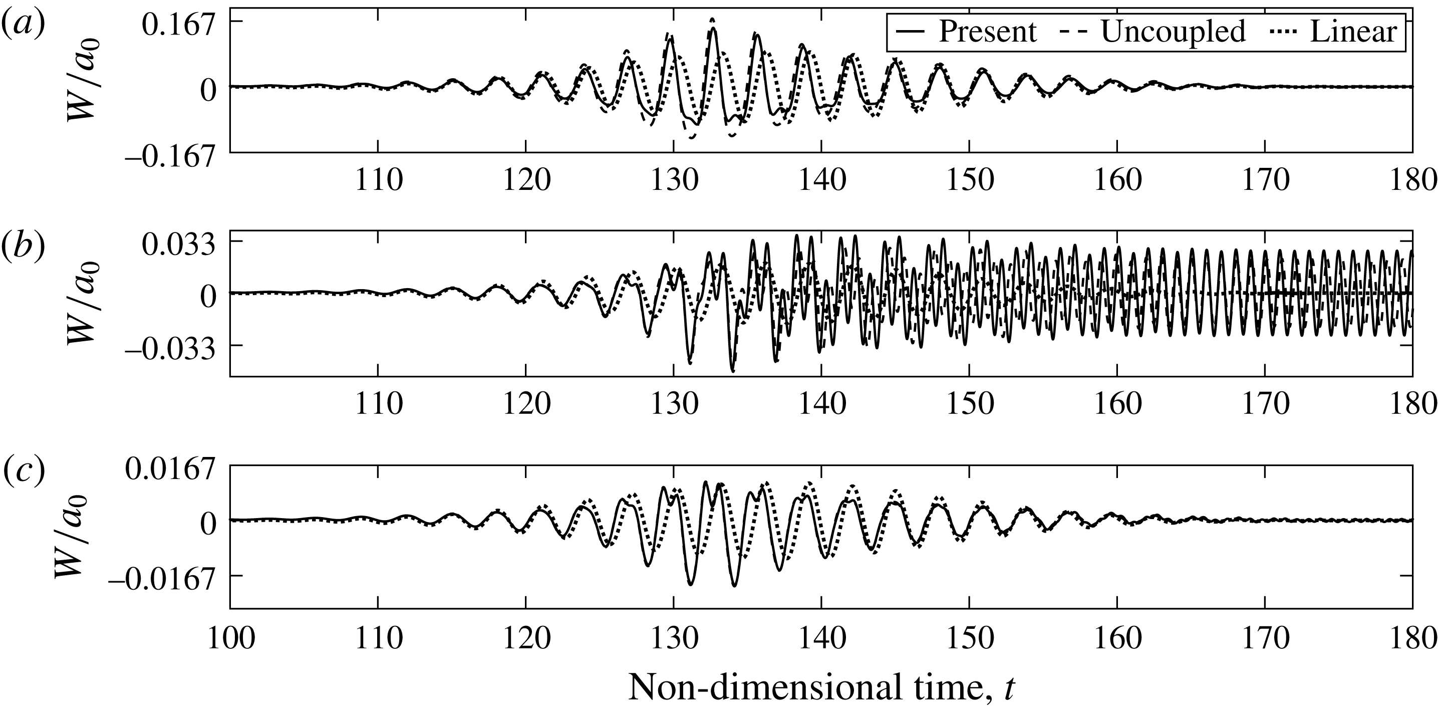
, are discussed. The results of the simulations are given in terms of the wave run-up in figure 14, the wave force in figure 15 and the wall’s motion at the mid-water depth in figure 16. Hydroelastic effects are immediately detected in the interaction results with the most flexible wall (
 $k_{s}=0.5$
). In this case, the results of the present spectral method show values’ relaxation compared with the results of the uncoupled analysis. On the other hand, the results of the two approaches are almost identical for the case of interaction with the stiffest wall (
 $k_{s}=3$
). In this case the effect of the wall’s response on the hydrodynamic values is weak, but in both cases the nonlinear effects lead to a significant deviation of the present results from the results of the linear analysis. The hydrodynamic and structural results of the present method reveal higher values and show a different pattern of oscillations. These differences are attributed to the contribution of higher wave harmonics, which are generated and amplified through resonant interactions between wave components of the incident group during the evolution stage (Carbone et al.
Reference Carbone, Dutykh, Dudley and Dias2013; Viotti, Carbone & Dias Reference Viotti, Carbone and Dias2014; Akrish et al.
Reference Akrish, Rabinovitch and Agnon2016a
,Reference Akrish, Schwartz, Rabinovitch and Agnon
b
). The initial narrow spectrum of the incident group (controlled by
 $\unicode[STIX]{x1D707}$
) becomes wider, a process that results in wave amplification along the flume and eventually leads to higher wave run-ups, as demonstrated by the present results in figure 14. The contribution of the higher harmonics to the wave force, and thus to the wall’s motion, causes multiple peaks at the locations of significant wave run-ups, as shown in figures 15 and 16.
The normalized wave group force,
 $F/F_{0}$
, on the wall using the present spectral method, the uncoupled analysis and the linear analysis for the following values of flexural stiffness: (a)
 $k_{s}=0.5$
, (b)
 $k_{s}=1.85$
, (c)
 $k_{s}=3$
.

The normalized wall’s motion at the mid-water depth,
 $W/a_{0}$
, using the present spectral method, the uncoupled analysis and the linear analysis for the following values of flexural stiffness: (a)
 $k_{s}=0.5$
, (b)
 $k_{s}=1.85$
, (c)
 $k_{s}=3$
.

An exceptional oscillation pattern is revealed in the interaction results with the wall whose flexural stiffness is
 $k_{s}=1.85$
. In this case, the third-order harmonics of the wave group lead to a resonant interaction (as also shown in figure 10). Obviously, this scenario cannot be predicted by the linear analysis, which does not account for the generation of the higher harmonics. Discrepancies are also found between the present and the uncoupled results. The reasons for these discrepancies stem from several simplifying assumptions adopted in the latter. First, the uncoupled analysis disregards the effect of the wall’s response on the hydrodynamic values. Therefore, the effect of the resonant interaction on the run-up (figure 14
b) and on the wave force (figure 15
b) appears only through the present results. Second, the uncoupled analysis ignores the effect of surface waves on the added-mass components by adopting the high-frequency approximation. And third, the uncoupled analysis disregards the effect of the amplification in wave pressure on the wall’s motion.
It is desired to close the discussion with a final remark regarding the decay rate of the wall’s oscillations. The decay of the oscillating wall is taken into account in the model of the present study through wave radiation. However, owing to its high eigenfrequencies, the wall generates wave energy that radiates at a fairly slow pace. Therefore, the effect of decay is hardly detected in figure 16(b). Obviously, this mechanism is totally neglected by the uncoupled analysis as a result of the high-frequency approximation.
5 Conclusions
This study has investigated the interaction of water waves and an elastic wall over constant water depth. The investigation has been carried out numerically in a two-dimensional flume-like computational domain. The simplicity of the domain has allowed us to perform highly efficient numerical simulations through spectral methods. For the solution of the fluid, the high-order spectral method (HOSM) has been applied, whereas the mode expansion method (MEM) has been used to solve the motion of the wall. The efficiency of this newly developed numerical code has been utilized to study several hydroelastic and nonlinear effects that arise in two cases of interaction. The first case focused on the interaction between a pulse-type wave and a rigid wall supported by lateral springs. The second case studied the interaction of an incident wave group and a deformable cantilever (fixed–free) wall.
The results of the first case of interaction revealed an interesting and unexpected phenomenon. The maximum wave run-up and wave force demonstrate prominent fluctuation around the values corresponding to a fixed wall, as a function of the wall’s eigenfrequency,
 $\unicode[STIX]{x1D714}_{n}$
. In order to explain this behaviour, extreme situations have been selected and analysed. It has been found that the mechanism leading to such extreme scenarios is the constructive interference between corresponding phases of the wall and the fluid motion. Accordingly, the lower points of maximum wave run-up and wave force (the values’ relaxation points) occur when the corresponding phases of the wall and the fluid motion interfere destructively.
Hydroelastic effects also play an important role in the second case of interaction. In particular, the following results are highlighted. First, hydroelastic effects were found to be crucial to evaluate the eigenfrequencies of the wall, and therefore to correctly predict the occurrence of resonant interactions. Second, they also lead to relaxation or amplification of the wall’s oscillations. These effects arise due to the influence of the wall’s response on the hydrodynamic pressure, which in turn relaxes or amplifies the oscillations. Finally, hydroelastic effects are necessary to quantify the hydrodynamic values. In a resonant interaction, as in an impact scenario, hydroelastic effects together with the effect of nonlinearity can lead to an extreme wave force and run-up. Such an extreme scenario has been demonstrated in the resonant interaction case due to second-order excitation.
The hydroelastic and nonlinear phenomena, which have been revealed through the interaction scenarios investigated in this study, can be crucial for the design of flexible structures exposed to violent wave fields. The study only takes an initial step towards looking into these phenomena, by considering simple structural models and non-breaking waves. Future studies should focus more on the quantitative significance of these phenomena under non-breaking and breaking wave conditions.
Acknowledgements
This study was supported by the Israel Ministry of Science, Space and Technology, contract no. 605404541.