1. Introduction
In the past decade, 3D light detection and ranging (LiDAR) sensors have received widespread attention and developed rapidly. Credited to its high resolution, high precision, and strong anti-interference ability, LiDAR(-inertial) odometry has been extensively studied. It is widely applied in many fields, such as self-driving vehicles [Reference Zhang, Wang, Jiang, Zeng and Dai1], autonomous unmanned aerial vehicles (UAVs) [Reference Li, Savkin and Vucetic2], and intelligent service robots. In the LiDAR-inertial odometry (LIO) system, local map maintenance is one of the critical blocks. The quality of the local map and the reconstruction of the SLAM system vary in different environments [Reference Fasiolo, Scalera and Maset3]. Maintaining a high-precision local map is significant to the accuracy of the LIO system. A classic method of mapping is KD-Tree [Reference Bentley4, Reference Friedman, Bentley and Finkel5]. Due to its computational efficiency, KD-Tree is widely used in LiDAR-based odometry. LOAM [Reference Zhang and Singh6], on which a series of recent works are based, constructs the map online by registering the raw LiDAR points into a local point cloud map using KD-Tree. To improve the efficiency, LOAM has to perform downsampling to reduce the points in the point cloud map. Moreover, KD-Tree is widely applied in the derivate method of LOAM, e.g., Lego-LOAM [Reference Shan and Englot7], LIO-SAM [Reference Shan, Englot, Meyers, Wang, Ratti and Rus8], and LINS [Reference Qin, Ye, Pranata, Han, Zhang and Liu9].
However, the KD-Tree structure has a nonnegligible limitation: the cost of reconstructing increases rapidly as the local map increases. To overcome the defect of the reconstruction cost, Fast-LIO2 [Reference Xu, Cai, He, Lin and Zhang10] introduces incremental KD-Tree (ikd-Tree) structure to the LIO system, which enables incremental updates and dynamic re-balancing. Compared with KD-Tree, ikd-Tree significantly reduces the computation load and improves efficiency. Based on iKD-Tree, Point-LIO [Reference He, Xu, Chen, Kong, Yuan and Zhang11] proposes a point-by-point state update, which fuses a LiDAR point at its actual sampling time without accumulating into a frame. This strategy allows Point-LIO to enormously increase the odometry rate and bandwidth significantly.
Faster-LIO [Reference Bai, Xiao, Chen, Wang, Zhang and Gao12] further improves the efficiency of mapping by introducing a sparse incremental voxel structure, which splits the local map into a hash-indexed voxel map to achieve a higher tracking speed. Unlike the tree-like structure, Faster-LIO stores the point cloud in hash-indexed sparse voxels and allows high-speed incremental addition and deletion, which is very computationally cheap for real-time LIO algorithms. AdaLIO [Reference Lim, Kim, Kim and Myung13] further imports an adaptive strategy in Faster-LIO, adaptively adjusts internal parameters by checking degeneracy and wins first place in the Hilti SLAM Challenge 2023.
LiTAMIN [Reference Yokozuka, Koide, Oishi and Banno14] develops a fast and light registration method, where the traditional ICP method [Reference Besl and McKay15] is stabilized with normalization of the cost function by the Frobenius norm and a regularized covariance matrix. LiTAMIN2 [Reference Yokozuka, Koide, Oishi and Banno16] further reduces the number of registered points and applies symmetric KL-divergence to ICP matching. Such strategy, however, leads to a decrease in accuracy compared with the traditional GICP [Reference Segal, Haehnel and Thrun17] method.
With further research facilitating, this point-based mapping structure does not satisfy the demands of describing the environment characteristics and the uncertainty of the point cloud. Consequently, a range of voxel mapping methods is proposed.
VGICP [Reference Koide, Yokozuka, Oishi and Banno18] extends the generalized iterative closest point (GICP) approach with voxelization. The pose optimization in VGICP is processed parallel to avoid costly nearest-neighbor searches employing the voxelization approach. Moreover, the voxel distributions are estimated by aggregating the distribution of each point in the voxel, which yields valid voxel distributions even when there are few points in a voxel.
Ba-liom [Reference Li, Zhang, Zhang, Yuan, Liu and Wu19] introduces adaptive voxel maps into LIO-SAM to mitigate the problem of undesired ground warping due to sparsity of laser scans and significantly reduce odometry drift.
Inspired by the normal distribution transformation [Reference Biber and Straßer20], VoxelMap [Reference Yuan, Xu, Liu, Hong and Zhang21] proposes an adaptive-size and coarse-to-fine voxel construction method based on octo-tree structure, which adds plane assumption in the voxel, and further estimate the covariance of the plane which achieve excellent performance in robustness and efficiency. VoxelMap++ [Reference Wu, You, Yuan, Kong, Zhang, Li and Zhao22] promotes the plane fitting and covariance estimation method in Voxelmap from 6DOF to 3DOF and proposes a novel online voxel merging method, arising the plane fitting accuracy. The shortcoming of these voxel-based methods is their significant calculation of resource consumption. The CPU usage of VoxelMap++ can reach up to 700%, yet under the same conditions, the CPU usage of Fast-LIO2 is just about 50%.
Nevertheless, these voxel-based methods also have limitations. In the voxel mapping method, there is often no connection between voxels. VoxelMap only considers segmenting large voxels based on planar features without considering other features and merging between voxels. In contrast, VoxelMap++ only merges voxels with plane features, regardless of voxels without plane features.
Meanwhile, in methods that implement feature-based or distribution-based registration metrics, point clouds are discarded if there is no target feature or distribution, which is harmful to the robustness of the system.
In this work, we address these issues by proposing two novel techniques: Incremental mergeable voxel and adaptive point matching method. More specifically, our contributions are as follows:
-
(i) A novel dynamic voxel smoothing method that allows online voxel smoothing without reducing computational efficiency. To achieve this goal, a cache of point cloud is set for each voxel to store the latest registered points. These points in the cache are to be added to this voxel to calculate the probabilistic model or replace the old points in the voxel if necessary. This approach is proposed from the perspective of engineering implementation, avoiding the blurriness of the local map, which is usually caused by accumulated odometry errors.
-
(ii) A promotion of the online voxel merging method in VoxelMap++, which allows the neighbor voxels to be connected or disconnected flexibly according to their similarity. Based on the voxel smoothing method, the voxels in this work are dynamically transforming, and due to the measurement noise and the FoV (Field of View) of the LiDAR sensor, a plane feature could only emerge after the corresponding voxels are merged. Thus, the voxel merging method is promoted not only for planar features but also for non-planar features. Moreover, a feature in a Union can also be removed once transformed dramatically. As shown in the experiment, this promotion has little impact on the system’s efficiency.
-
(iii) An adaptive feature matching method to ensure a high points matching rate. This approach provides k nearest points search for fitting a local plane facet for the area that has not been sufficiently explored. In the meantime, local features are extracted from the nearby voxels to address the measurement model for the sufficiently explored area. This approach is also proposed from the engineering implementation perspective and is proven valid for improving system robustness.
2. Methodology
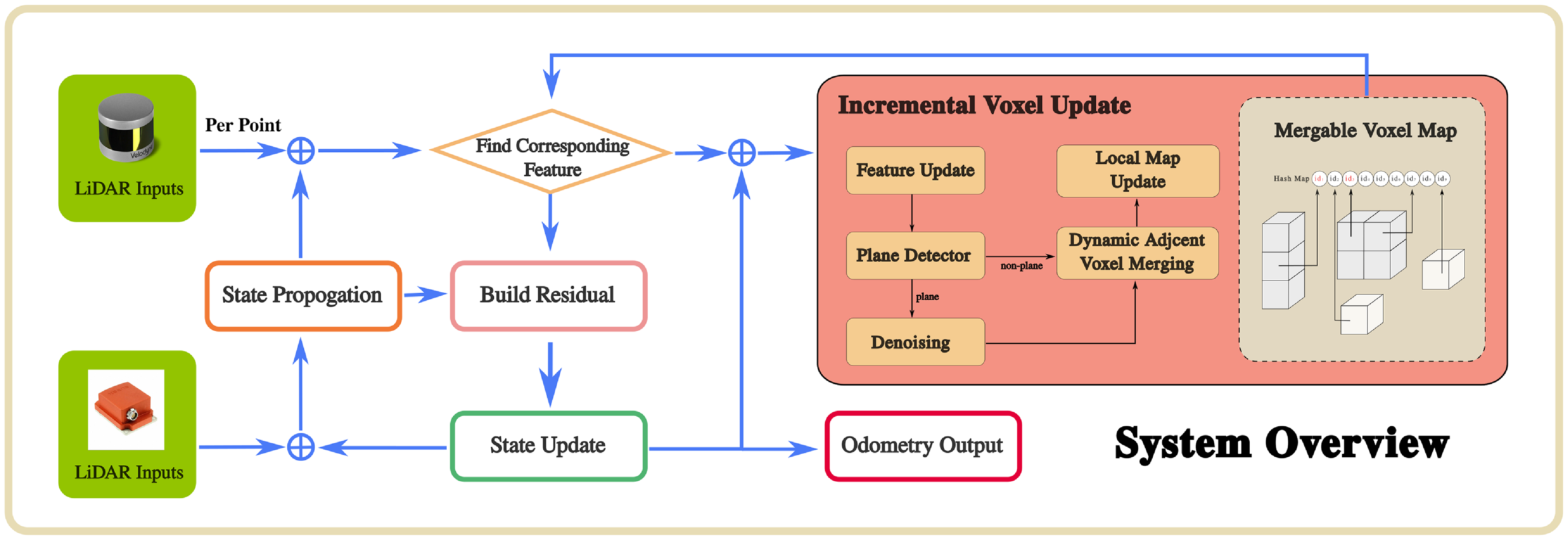
The pipeline of DV-LIO is shown in Figure 1. For each LiDAR point received, a corresponding voxel that contains a plane feature from the voxel map is searched. If successfully matched, a residual is computed to update the system state. If not, the nearest neighbor points will be searched to fit a local plane facet to calculate the residual. The optimized pose finally registers the LiDAR point into the global frame, registers to the local map, and proceeds to the next LiDAR Point. Otherwise, the Kalman filter-predicted pose directly registers it to the local map. After registering all the points in the received scan to the local map, smoothing and merging evaluations are performed on all the varying voxels.
System overview.

2.1. Data structure of dynamic voxel
The voxel map method based on sparse hash indexing is a lightweight and flexible map management model. In our map management strategy, we maintain local environmental information in the voxel map. As the basic theory of the voxel structure in DV-LIO, the noise model of the laser point is first obtained based on the observation model of the LiDAR sensor. After modeling the uncertainty of the point cloud, the voxel structure, along with the voxel smoothing and merging method, could be carried out.
2.1.1. Uncertainty of LiDAR points
The uncertainty of the point cloud result from LiDAR measurement noises should first be described to form the probabilistic model of the voxel map. As is shown in ref. [Reference Yuan, Xu, Liu, Hong and Zhang21], the uncertainty of each point received from LiDAR is determined by the ranging uncertainty and bearing direction uncertainty. The noise
 $\delta p_i$
of the measured point
 $p_i$
and its covariance
 $\Sigma _{p_i}$
follow:
 \begin{align} \delta _{p_i} &= \begin{bmatrix} \omega _i & -d_i{[\omega _i]}_\wedge N(\omega _i) \end{bmatrix} \begin{bmatrix} \delta _{d_i} \\ \delta _{\omega _i} \end{bmatrix} \sim \mathcal {N}(0,\Sigma _{p_i} ) \end{align}
 \begin{align} \Sigma _{p_i} &= \begin{bmatrix} \omega _i & -d_i{[\omega _i]}_\wedge N(\omega _i) \end{bmatrix} \begin{bmatrix} \Sigma _{d_i} & \\ & \Sigma _{\omega _i} \end{bmatrix} \begin{bmatrix} \omega _i & -d_i{[\omega _i]}_\wedge N(\omega _i) \end{bmatrix}^T \end{align}
where
 $\omega _i$
is the measured bearing direction of LiDAR,
 $\delta _{\omega _i}\sim \mathcal {N}(0,\Sigma _{\omega _i} )$
is the bearing direction noise in the tangent plane of
 $\omega _i$
, and
 $\delta _{d_i} \sim \mathcal {N}(0,\Sigma _{d _i})$
is the be the ranging noise of LiDAR.
 $N(\omega _i) = \begin{bmatrix} N_1 & N_2 \end{bmatrix} \in \mathbb {R}^{3 \times 2}$
is an orthonormal basis of the tangent plane at
 $\omega _i$
,
 ${[\cdot ]}_\wedge$
denotes the skew-symmetric matrix mapping the cross product. Detailed derivation of equation (1) and (2) can be found in refs. [Reference Yuan, Xu, Liu, Hong and Zhang21, Reference Liu and Zhang23]. The point
 $^{L}p_i$
and its covariance
 $\Sigma {^{L}p_i}$
could be further mapped to the world coordinate system utilizing the system state:
 \begin{equation} \begin{aligned} &^{\omega }p_i = {^{\omega }R_L} \cdot {^{L}p_i} + {^{\omega }t_i} \\ &\begin{aligned} \Sigma ^{\omega }p_i = &{^{\omega }R_L} [^{L}p_i]_ \wedge \Sigma _R [^{L}p_i]_ \wedge ^T {^{\omega }R_L^T} \\ + &{^{\omega }R_L} \Sigma {^{L}p_i}{^{\omega }R_L^T} +\Sigma _t \end{aligned} \end{aligned} \end{equation}
2.1.2. Modeling
To perform accurate point matching for the measurement model of the system, we differentiate the feature of the voxel, i.e., the centroid
 $\bar {p}_v$
of the point cloud
 $p_i(i=1,2\dots n)$
and the covariance matrix
 $\Sigma _v$
, by its probabilistic model as is computed following (4).
 \begin{equation} \begin{aligned} &\bar {p}_v = \frac {1}{n} \sum _{i=1}^n p_i \\ & \Sigma _v = \frac {1}{n} \sum _{i=1}^n (p_i - \bar {p}_v)(p_i -\bar {p}_v)^T \end{aligned} \end{equation}
By performing SVD decomposition on the covariance, the point cloud distribution within the voxel can be obtained: the larger the eigenvalues, the more dispersed the point clouds are in the corresponding eigenvector direction. According to different voxel probabilistic models, we classify voxel features into three types: linear, planar, and ellipsoid.
In order to distinguish them, 2 indexes are utilized. Assuming that the eigenvalues of the matrix are
 $\lambda _{1}$
,
 $\lambda _{2}$
, and
 $\lambda _{3}$
in descending order, we introduce
 $\sigma _{2D}$
along with
 $\lambda _{3}$
to classify the voxel feature [Reference Dellenbach, Deschaud, Jacquet and Goulette24]:
 \begin{equation} \sigma _{2D} = \frac {\lambda _{2} - \lambda _{3}}{\lambda _{1} - \lambda _{2}}. \end{equation}
Larger
 $\sigma _{2D}$
indicates that the feature is more likely to be a plane. Thus, the feature is classified as a plane when its
 $\sigma _{2D}$
is larger than the plane threshold
 $\sigma _{thr}$
. If
 $\sigma _{2D}$
is smaller than
 $\sigma _{thr}$
, the feature would be classified as linear if
 $\lambda _{3}$
is smaller than 0.001, or ellipsoid otherwise.
2.2. Voxel update
2.2.1. Dynamic voxel smoothing
To prevent overfitting, each voxel only contains at most 50 points, and a specific interval between the points is required to ensure the scattered distribution of the point cloud. However, it could be computationally expensive if the voxels are updated every time the new point comes. Thus, we set up a buffer queue
 $q_{tmp}$
in the voxel. The newly registered points will not directly affect the probabilistic model but will first enter
 $q_{tmp}$
. The voxel will be updated after sufficient points are accumulated.
When updating the voxel, the points in
 $q_{tmp}$
will be registered to the current voxel, and the probabilistic model of the voxel will be updated incrementally according to (6):
 \begin{equation} \begin{aligned} & \bar {p}_{v_{\text {upd}}} = \frac {n}{m+n} \bar {p}_{v_{\text {ori}}} + \frac {n}{m+n} \bar {p}_{tmp} \\ & \begin{aligned} \Sigma _v = &\frac {n}{m+n} \left [ \Sigma _{v_{\text {ori}}} + (\bar {p}_v - \bar {p}_{v_{\text {ori}}})(\bar {p}_v - \bar {p}_{v_{\text {ori}}})^T \right ] \\ & + \frac {m}{m+n} \left [ \Sigma _{p_{\text {tmp}}} + (\bar {p}_v - \bar {p}_{tmp})(\bar {p}_v - \bar {p}_{tmp})^T \right ] \end{aligned} \end{aligned} \end{equation}
where
 $\bar {p}_{v_{\text {ori}}}$
and
 $\Sigma _{v_{\text {ori}}}$
denote the origin center and covariance of the current voxel,
 $\bar {p}_{v_{\text {upd}}}$
and
 $\Sigma _{v_{\text {upd}}}$
denote the centroid and covariance matrix, respectively, after updated,
 $n$
,
 $m$
are the number of points in the voxel and the
 $q_{tmp}$
, respectively.
 $\bar {p}_{tmp}$
and
 $\Sigma _{p_{\text {tmp}}}$
are the center and covariance of points in
 $q_{tmp}$
calculated according to (4).
Notice that the number of point clouds may exceed 50 after the update. In this case, it is necessary to remove the excess points. To reduce the interference of noise points while ensuring feature accuracy, normalized Mahalanobis distance is used to describe the degree to which the point cloud conforms to the probabilistic model of the current voxel:
 \begin{equation} \rho _{p_i} = \frac {\| p_i - \bar {p}_v \|_{\Sigma _p + \Sigma _v}}{(p_i - \bar {p}_v)^T (p_i - \bar {p}_v)} \end{equation}
To remove those points that do not comply with the probabilistic model of the current voxel, all the points in the voxel will be sorted according to their
 $\rho$
, and those points with larger
 $\rho$
will be removed. Then, the probabilistic model is to be refined according to (8):
 \begin{equation} \begin{aligned} &\bar {p}_v = \frac {n}{n-l} \bar {p}_{v_{\text {upd}}} + \frac {l}{n-l} \bar {p}_{rm} \\ & \begin{aligned} \Sigma _v = &\frac {n}{n-l} \left [ \Sigma _{v_{\text {upd}}} + (\bar {p}_v - \bar {p}_{v_{\text {upd}}})(\bar {p}_v - \bar {p}_{v_{\text {upd}}})^T \right ] \\ & - \frac {l}{n-l} \left [ \Sigma _{v_{\text {rm}}} + (\bar {p}_v - \bar {p}_{rm})(\bar {p}_v - \bar {p}_{rm})^T \right ] \end{aligned} \end{aligned} \end{equation}
where
 $\bar {p}_{rm}$
and
 $\Sigma _{v_{\text {rm}}}$
are the center and the covariance of the points to be removed, and
 $l$
is the number of them.
2.2.2. Real-time merging and segmenting method
The voxel map framework based on sparse hash index used in this article is similar to Faster-LIO [Reference Bai, Xiao, Chen, Wang, Zhang and Gao12] and uses hash index to maintain the voxel based local map. This map maintenance method has high search efficiency due to its sparsity and hash index based characteristics, but it also loses the feature correlation between adjacent voxels. Inspired by VoxelMap++ [Reference Wu, You, Yuan, Kong, Zhang, Li and Zhao22], this work introduces a voxel management mechanism based on feature distribution to unify the features of adjacent similar voxels. The voxel management mechanism determines whether merging can be performed based on the similarity between voxels. However, unlike the method used in VoxelMap++, the proposed method uses a hash-based sparse voxel map, which does not have innate associations between voxels. Therefore, it is necessary to design a neighboring voxel search strategy to find the target voxel for merging detection. Moreover, the proposed method does not compress the point cloud into a plane but rather uses the Hellinger distance to determine the similarity between voxels and perform voxel merging without sacrificing the accuracy of the original point cloud features.
To perform voxel merging on the current voxel
 $V_{cur}$
, the search direction is to be specified using the current voxel features. Notice that it is more likely to find target voxels to be merged in the direction where the point cloud has a higher density, the search direction is to be specified based on the eigenvector of the covariance matrix of the current voxel and its corresponding feature values (9).
 \begin{equation} \mathbf {d} = \frac {\lambda _1 \mathbf {n}_1 + \lambda _2 \mathbf {n}_2 + \lambda _3 \mathbf {n}_3}{\sqrt {{\lambda _1}^{2} +{\lambda _2}^{2} + {\lambda _3}^{2}}} \end{equation}
The searching area is fixed within the
 $9\times 9$
range around the current voxel. For this purpose, a list of 26 direction vectors is set, and each vector
 $d_i$
corresponds to the direction of the potential adjacent voxel
 $V_{adj_i}$
. The adjacent voxel
 $V_{adj_i}$
will only be searched when the dot product between
 $d$
and the corresponding direction vector
 $d_i$
is larger than 0.75.
Suppose
 $V_{adj_i}$
exists and has sufficient points that the probability model of it is stable enough. In such case, the Hellinger distance between
 $V_{adj_i}$
and
 $V$
will be calculated (10). If
 $s_{i}$
is smaller than 0.2, the two voxels are considered as congeneric voxels and will be merged.
 \begin{equation} s_{i} = \sqrt { \frac { {det(\Sigma _i)det(\Sigma )}^{\frac {1}{2}} } {det(\frac {\Sigma _i + \Sigma }{2})} } \end{equation}
There are two conditions for merging. First, if neither of the congeneric voxels has been merged, one of the voxels is to be set as the root node, and the probability model of the merged entire will be stored in it. Meanwhile, the other is the leaf node linked to the root. Otherwise, if at least one voxel has been merged, the Mahalanobis distance between them is considered, and only when the Mahalanobis distance between the two is less than 0.2 can the two be merged. If one of them has not been merged, it will be directly set as a leaf node and linked to the root of the other. If all of them are merged, the root node with fewer leaf nodes will be downgraded as a leaf node to the other, and all its leaf nodes will be transferred to the other root.
When performing voxel merging, one voxel is set to be the root node of the distribution. The root node contains a leaf-list of neighboring voxels with the same distribution. The root node also includes the probabilistic model of the whole. Meanwhile, all updates operated to leaf nodes must also be synchronized to the entire when performing voxel updating.
Also, there is sometimes a situation in which a leaf node no longer belongs to the origin distribution. In such case, the leaf node is to be cut, and the probabilistic model of the origin distribution will be refined.
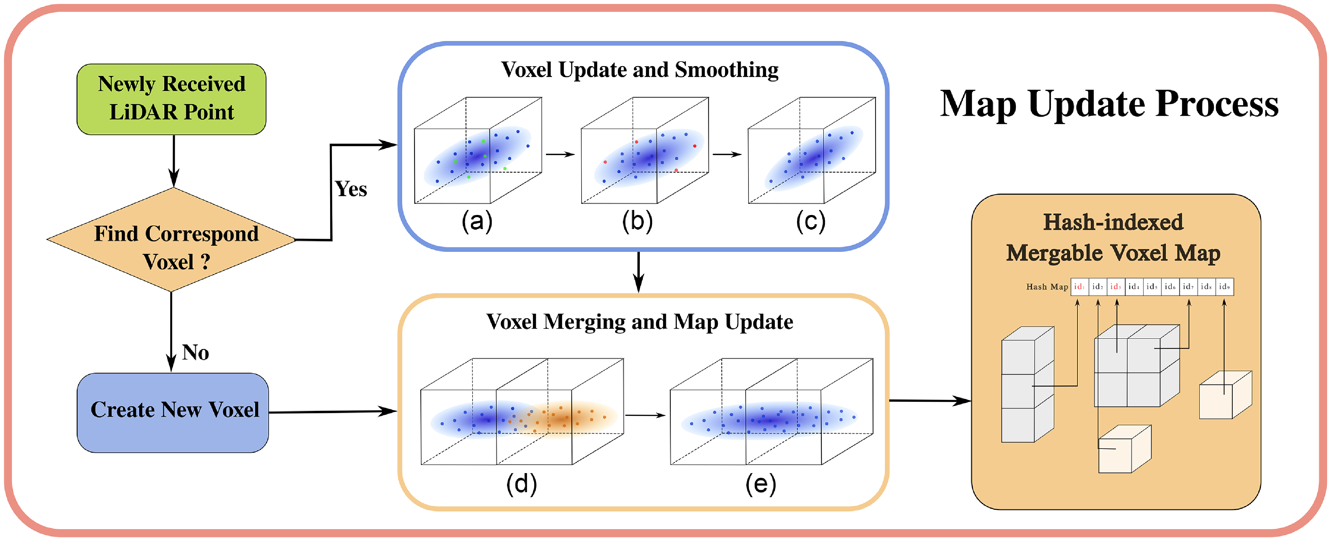
Figure 2 shows the entire map updating process. When registering a newly received LiDAR point to the map, the first step is to find if the corresponding voxel exists. If not, a new voxel will be created, and the point will be registered. Otherwise, the point will be stored in the
 $q_{tmp}$
of the corresponding voxel, and the voxel will be updated and smoothed if it meets the update condition. Then, the neighbor voxels located in the search direction in (9) will be queried to perform voxel merging or segmenting. Finally, the local map is updated.
Map updating process; a)-c): Voxel smoothing process, where a) is the voxel with newly registered points (green), b) shows the points to be deleted, and c) is the voxel after updated; d)-e): voxel merging process, where d) illustrates two congeneric voxels to be merged, and e) is the merging result.

3. Point matching
In this section, we are to expound on the idea of matching a LiDAR point with the local map to construct the constraint for the state estimation.
Assume that the LiDAR frame coincides with the body frame. A LiDAR point
 $^{L}p_{k+1}$
is the true position in the LiDAR coordinate frame. After projected to the global frame with the true body pose, the point
 $^{L}p_{k+1}$
should lie exactly on a plane feature or a local plane facet, which could be described as
 \begin{equation} 0 = ^{G}\mathbf {\mu }_k^T[^{G}R_L(^{L}p_{k+1})+^{G}t_L-^{G}q_{k+1}] \end{equation}
where
 $^{G}\mathbf {\mu }_{k+1}$
is the normal vector of the corresponding plane feature or facet.
The plane or the facet is obtained from the nearest voxels. First, we will search the nearest voxels in the local map for a plane or line feature. Suppose the feature has been found and is close to the target point. In that case, the eigenvector corresponding to the minimum eigenvalue of its covariance matrix is to be used as the normal vector
 $^{G}\mathbf {\mu }_{k+1}$
, and the centroid to be
 $^{G}q_{k+1}$
. Otherwise, the nearest five points within the searching range will be searched to fit the local plane facet for the Point-to-Plane matching in (11).
However, the true point
 $^{L}p_{k+1}$
can not be directly obtained due to the measurement noise
 $n_{L_{k+1}}$
of the LiDAR sensor. Let
 $^{L}\hat {p}_{k+1}$
be the observation of
 $^{L}p_{k+1}$
, it can be denoted as
 \begin{equation} ^{L}\hat {p}_{k+1} = ^{L}p_{k+1} + n_{L_{k+1}} \end{equation}
Similarly, the uncertainty of the fitted plane also needs to be modeled. Both plane feature and facet consist of a group of points
 $^{\scriptscriptstyle {G}\!}\!p_i$
(
 $i=1,2,\dots, N$
). Because there is no essential difference between a plane feature and a facet, no further distinction will be made in the following discussion, and both of them will be denoted as a plane. The center point
 $^{\scriptscriptstyle {G}\!}\!\bar {p}$
and the eigenvector associated with the minimum eigenvalue of the plane covariance can be denoted as functions of
 $^{\scriptscriptstyle {G}\!}\!p_i$
as
Assume the covariance of the plane has the eigenvector matrix
 $U$
, the derivative of the
 $^{\scriptscriptstyle {G}\!}\!\bar {p}$
and
 $^{\scriptscriptstyle {G}\!}\!\mu$
with respect to each point in
 $^{\scriptscriptstyle {G}\!}\!p_i$
as below:
 \begin{align} \,[^ {G}\!\mu, ^{G}\!\bar {p}]^T &= f(^{G}\!p_1 + \delta ^{G}\!p_1, ^{G}\!p_2 + \delta ^{G}\!p_2, \ldots, ^{G}\!p_n + \delta ^{G}\!p_n) \nonumber\\ &\approx \,[\mu, \bar {p}]^T + \sum _{i=1}^N \frac {\partial f}{\partial ^{G}\!p_i} \delta ^{G}\!p_i \end{align}
 \begin{equation} \begin{aligned} \frac {\partial \mu }{\partial ^{\scriptscriptstyle {G}\!}\!p_i} = U \begin{bmatrix} F_{1,3}^{P_i} \\ F_{2,3}^{P_i} \\ F_{3,3}^{P_i} \end{bmatrix}, &F_{m,3}^{P_i} = \begin{cases} \frac {(^{\scriptscriptstyle {G}\!}\!p_{i} - \bar {{p}})^T}{N(\lambda _3 - \lambda _m)} (u_{m}\mu ^{T} + \mu u_{m}^T), & m \neq 3, \\ 0_{1 \times 3}, & m = 3. \end{cases}\\ \frac {\partial \bar {p}}{\partial ^{\scriptscriptstyle {G}\!}\!p_{i}} &= \text {diag} \left ( \frac {1}{N}, \frac {1}{N}, \frac {1}{N} \right ) \end{aligned} \end{equation}
Detailed derivation of equation (18) and (14) can be found in ref. [Reference Yuan, Xu, Liu, Hong and Zhang21]. And the covariance matrix
 $\Sigma _{\mu, \bar {p}}$
of normal vector
 $n$
and center
 $\bar {p}$
is therefore:
 \begin{equation} \Sigma _{\mu, \bar {p}} = \sum _{i=1}^N \frac {\partial f}{\partial ^{\scriptscriptstyle {G}\!}\!p_{i}} \Sigma _{\scriptsize {^{\scriptscriptstyle {G}\!}\!p_{i}}} {\frac {\partial f}{\partial ^{\scriptscriptstyle {G}\!}\!p_{i}}} ^T \end{equation}
Thus, the measurement model could be denoted as
 \begin{equation} 0 = h(x_{k+1}, ^{\scriptscriptstyle {L}}p_{k+1}, n_{L_{k+1}}, n_{pl_{k+1}}) \end{equation}
where
 $n_{pl_{k+1}} = [n_{\mu _{k+1}}, n_{q_{k+1}}]^{T}$
is the nosie of the corresponding plane.
4. State estimation
According to the measurement model in (16), a residual
 $r_{k+1}$
is calculated as
 \begin{equation} \begin{aligned} r_{k+1} &= 0 - h(\hat {x}_{k+1}, ^{L}\hat {p}_{k+1}, 0, 0) \\ &= h(x_{k+1}, ^{L}p_{k+1}, n_{L_{k+1}}, n_{pl_{k+1}}) - h_{L}(\hat {x}_{k+1}, ^{L}\hat {p}_{k+1}, 0, 0) \\ &\approx H_{k+1} \delta x_{k+1} + D_{L_{k+1}}n_{L_{k+1}} + D_{pl_{k+1}}n_{pl_{k+1}} \end{aligned} \end{equation}
where
 $\delta x_{k+1} = x_{k+1} \boxminus \hat {x}_{k+1}$
is the error state between the true state
 $x_{k+1}$
and the prior
 $\hat {x}_{k+1}$
of the true state. The prior
 $\hat {x}_{k+1}$
and its covariance
 $\hat {P}_{k+1}$
is propagated following directly the state transition model. This propagated state
 $\hat {x}_{k+1}$
and its covariance matrix
 $\hat {P}_{k+1}$
impose a prior Gaussian distribution of the true state
 $x_{k+1}$
as
 \begin{equation} \begin{aligned} \delta x_{k+1} &= x_{k+1} \boxminus \hat {x}_{k+1} \approx \mathcal {N}(0,\hat {P}_{k+1}) \end{aligned} \end{equation}
The residual (17) gives another Gaussian distribution for
 $\delta x_{k+1}$
:
 \begin{equation} \begin{aligned} &D_{k+1} n_{k+1} = r_{k+1} - H_{k+1} \delta x_{k+1} \approx \mathcal {N}(0,\bar {R}_{k+1}) \\ &\bar {R}_{k+1} = D_{k+1}R_{k+1}D_{k+1}^T \end{aligned} \end{equation}
Combining this state prior distribution in (18) and the measurement model (17) yields the posterior distribution of the state
 $x_{k+1}$
 \begin{equation} \arg \min _{\delta x_{k+1}} \left ( \| r_{k+1} - H_{k+1} \delta x_{k+1} \|^2_{\bar {R}_{k+1}} + \| \delta x_{k+1} \|^2_{\hat {P}_{k+1}} \right ) \end{equation}
The optimization problem in (20) can be solved by an extended Kalman filter. Detailed derivation can be found in [Reference He, Xu, Chen, Kong, Yuan and Zhang11].
5. Experiment
In this section, we evaluate the accuracy and efficiency of our system through a series of experiments. All the experiments are carried out on a laptop with an Intel i7-975H CPU (12 Cores, 2.60 GHz) and RTX 2060 GPU. Since this system is designed for a lightweight computing platform, which has limited RAM and computation performance, we set the size of the local map to L = 600 m.
The datasets used in experiments are drawn from three datasets that provide IMU and LiDAR measurement, that is, “m2dgr” [Reference Yin, Li, Li, Yu and Zou25], “nclt” [Reference Carlevaris-Bianco, Ushani and Eustice26], “newcollege” [Reference Smith, Baldwin, Churchill, Paul and Newman27], and ”botanicgarden” [Reference Liu, Fu, Qin, Xu, Xu, Chen, Goossens, Yu, Liu and Chen28]. The datasets of “m2dgr” include a series of sequences including challenging environments, such as long-term corridors, spacious outdoor venues, and moving obstacles. The “nclt” datasets propose a series of long-term campus sequences, including indoor and outdoor environments collected in different weather conditions. And “newcollege” datasets collect a sequence from a campus and a park nearby. Among them, “m2dgr”, “nclt”, and ”botanicgarden” use Velodyne HDL-32E LiDAR, and “newcollege” uses Ouster-128 LiDAR.
5.1. Efficiency
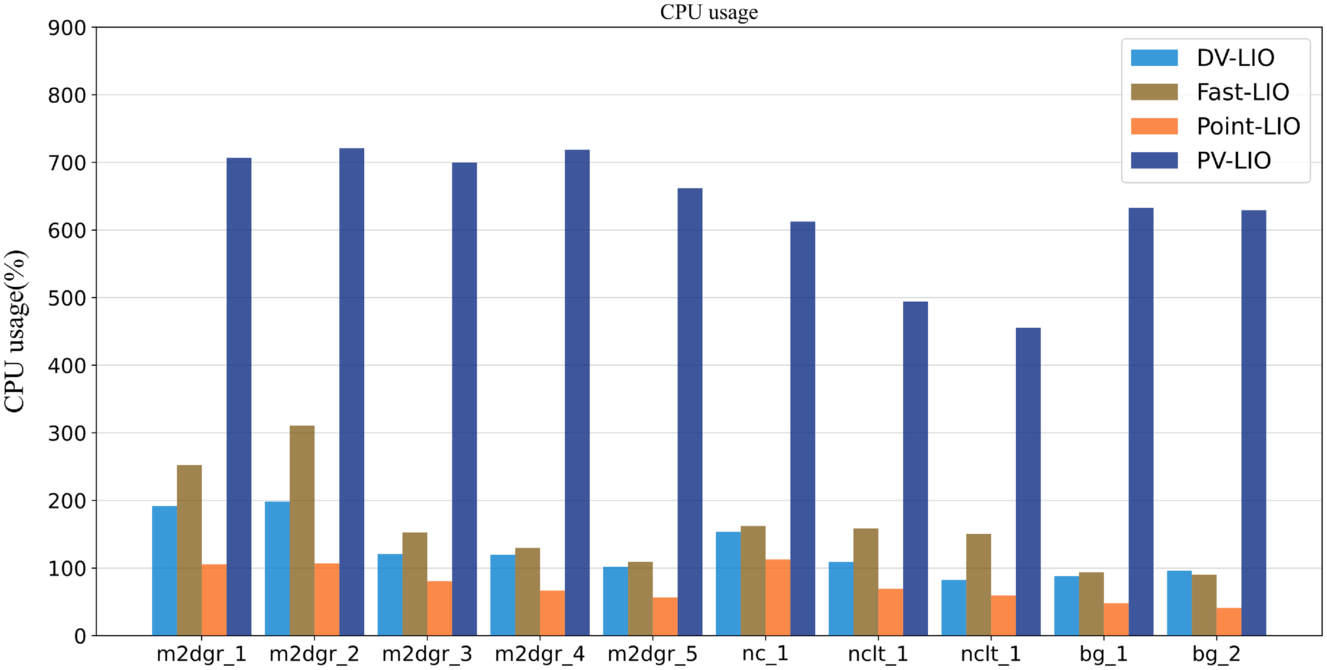
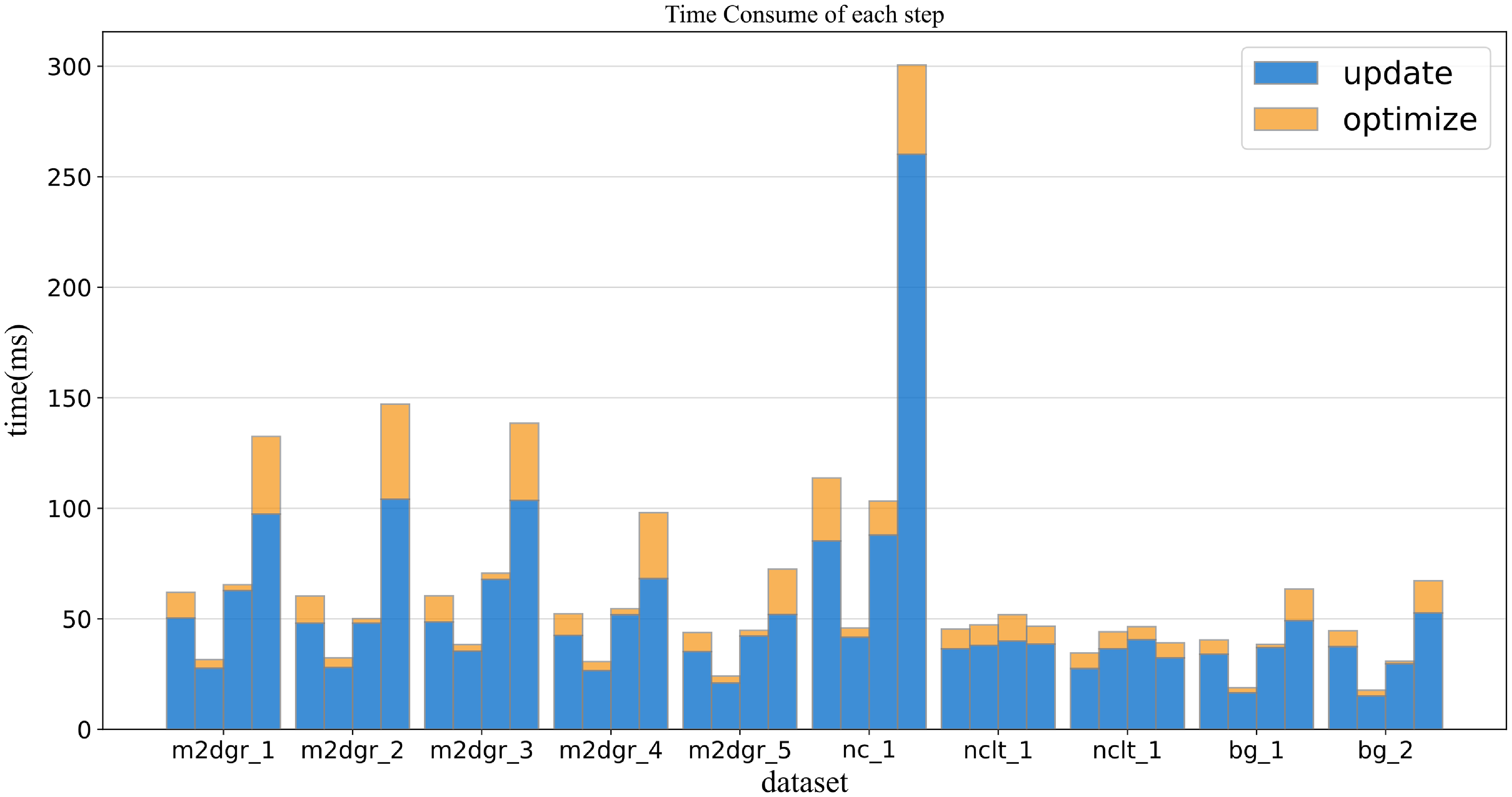
The efficiency of system optimization and map update is evaluated by computing the average runtime of each scan and the average number of effective points. In this section, we compare DV-LIO with Kalman filter-based methods, including Fast-LIO2, Point-Lio, and VoxelMap+Point-Lio. We investigate the time cost and the CPU usage of each algorithm step in LIO in Figs. 3 and 4.
CPU usage.

Time consume of each step.

Figure 3 compares CPU usage among four algorithms in different dataset sequences. Since all four algorithms do not use GPUs, the CPU usage comparison can well reflect the consumption of computing resources by the four algorithms. It can be seen that PV-LIO has a significantly higher CPU usage than other algorithms due to the need for high-frequency voxel segmenting and plane fitting. Meanwhile, DV-LIO, based on feature matching, has slightly higher CPU usage than Point-LIO and lower CPU usage than Fast-LIO. This is because DV-LIO adopts a point-to-point update strategy as in Point-LIO, which makes the observation model dimension extremely low during a single update process, effectively reducing computational resource consumption.
The CPU usage of DV-LIO varies in different environments. In the dataset with more buildings, i.e., “m2dgr” and “nclt”, the computational cost could be higher. Overall, the overall computational resource consumption is lower than that of Fast-LIO.
Figure 4 shows a comparison of the average time consumption of four algorithms during processing a LiDAR scan on different datasets. The time consumption illustrated in Figure 4 mainly consists of two parts. The optimizing process includes the time consumption for the construction of observation models and system updating, and the updating process includes the time consumption for state updating and map updating. This experiment only focuses on comparing the differences between DV-LIO and other algorithms in map maintenance and state updates. Thus, IMU forward propagation and point cloud preprocessing are not included.
DV-LIO uses the point-by-point update strategy, which requires a highly high update frequency. Thus, the time consumption of DV-LIO and Point-LIO is higher than that of Fast-LIO. Moreover, when constructing observation models, DV-LIO combines point-to-plane matching and point-to-facet matching for robustness, which increases the time consumption. However, the map update process of DV-LIO is faster than that of Point-LIO. Although DV-LIO employs a more complex map updating process than Point-LIO, the advantage of hash-indexed voxel map ensures its efficiency. Overall, the time consumption of DV-LIO and Point-LIO is roughly the same.
5.2. Accuracy
This section quantitatively presents a comparison of system accuracy.
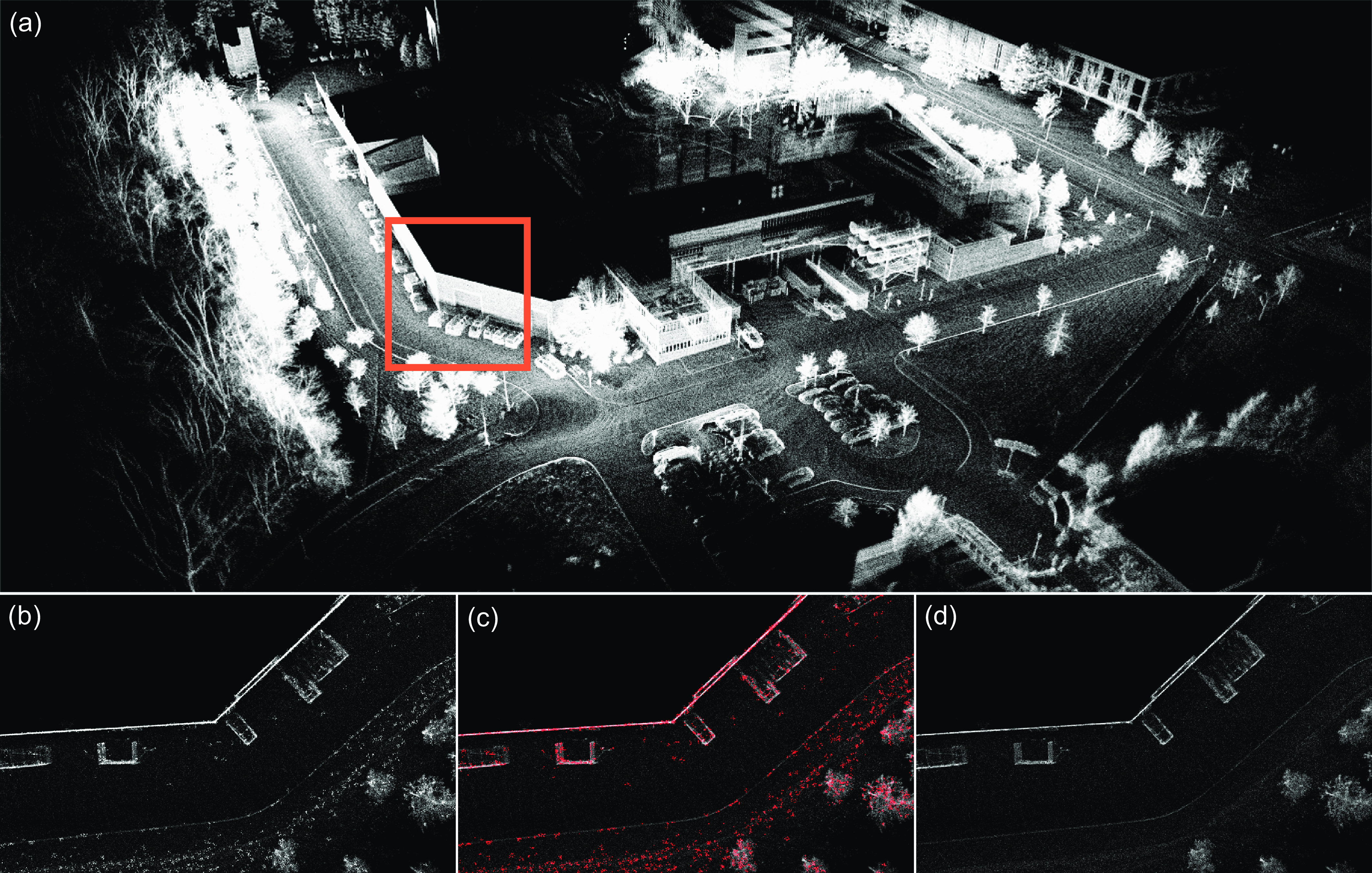
We first verify the effect of the dynamic voxel smoothing method by comparing the accuracy of mapping. Figure 5 shows the mapping result before and after voxel smoothing. As can be seen, there are a lot of noise points (marked as outliers in (c)) before voxel smoothing, resulting in thick walls and rough surfaces in (a). After the voxel smoothing, as is shown in (d), the thickness of the wall significantly reduces, and the surfaces of the features become much smoother.
Mapping result of DV-LIO in NCLT dataset. a): Local map; b): mapping result before voxel smoothing; c): points to be removed; d): mapping result after voxel smoothing.

We use absolute traditional pose error for drift evaluation. For this part, we compare the DV-LIO with FastLIO2, PointLIO, LIO-SAM, and VoxelMap+Point-LIO. Since DV-LIO does not have loop closure detection, we manually turn off the loop closure function in LIO-SAM for a fair comparison. The selected sequences all have good ground-truth trajectories collected by RTK sensors.
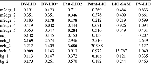
As reported in Table I, DV-LIO and DV-LIO* (DV-LIO with voxel merging) perform best in 7 out of 11 sequences. In environments with sufficient plane features like urban roads and campus streets (the sequence in m2dgr and nclt), DV-LIO with the voxel merging method could consistently achieve better accuracy. The system without the voxel merging method performs better in an environment containing only a few plane features besides the ground.
Comparison of RMSE (meters) for DV-LIO, DV-LIO*, FAST-LIO2, Point-LIO, and LIO-SAM on public sequences.

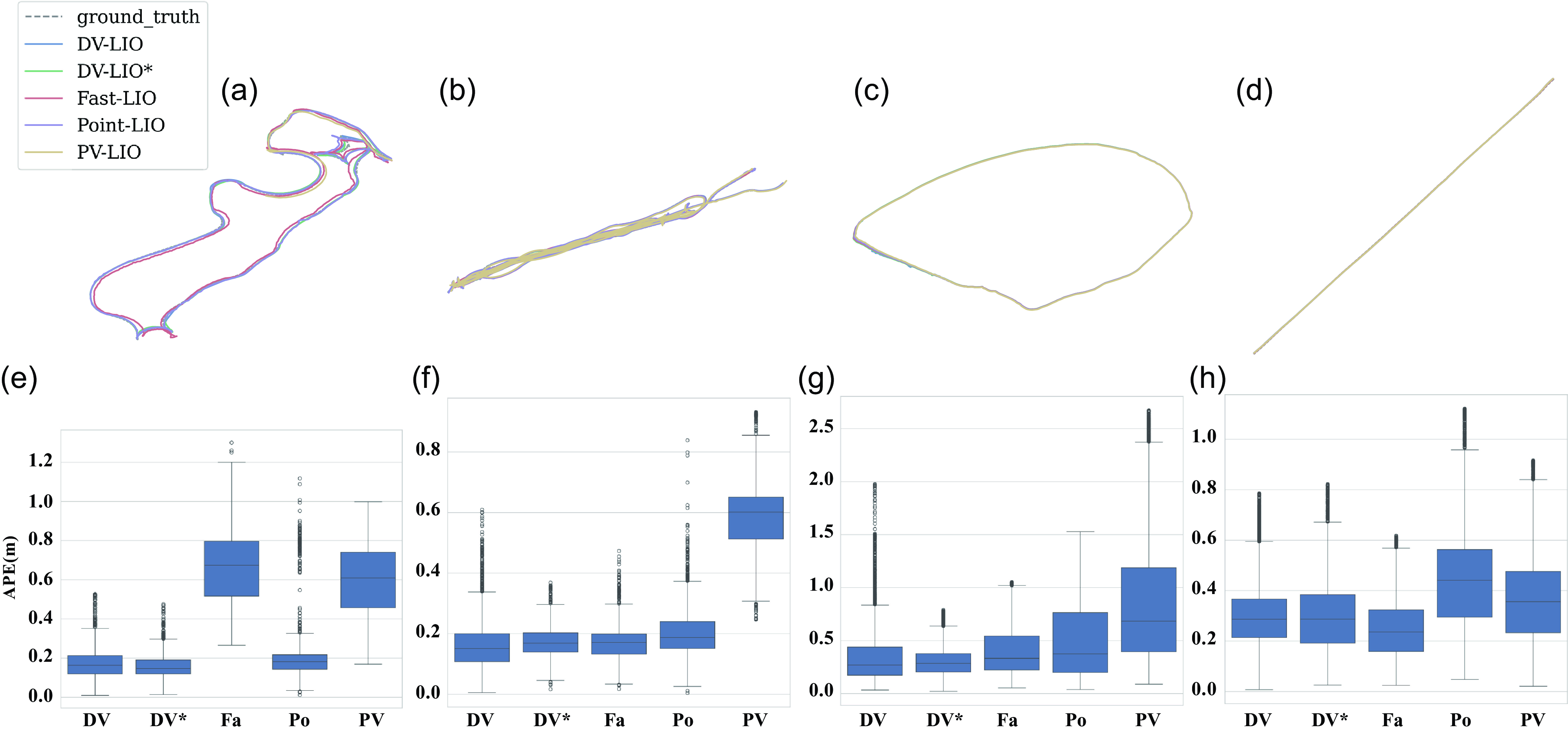
Figure 6 shows the entire mapping result and the box plot of the translation errors of DV-LIO, DV-LIO*, FastLio2, Point-LIO, and VoxelMap+Point-LIO.
Robustness compare. a)-d): Trajectory of DV-LIO, DV-LIO*, Fast-LIO, Point-LIO, and VoxelMap+Point-LIO; e)-h): box plot of the RMSE and its standard deviation of the compared methods in a)-d).

In the experiment shown in Figure 6, a), b), and c) are all outdoor campus environments with rich planar features, and d) for a long straight lane. It can be seen that in the three environments shown in a), b), and c), the proposed method achieved the best results in both mean and variance of errors, especially DV-LIO*, which achieved the minimum variance in e), f), and g). This result indicates that the proposed method can effectively improve the consistency of the map feature in environments with rich planar features, thereby significantly improving the accuracy performance of odometry. However, in the d) environment, although the method proposed in this paper still has significant advantages in terms of error mean and variance compared to other algorithms, it is slightly inferior to Fast LIO, and the error mean and variance of DV-LIO are also better than DV-LIO*. The reason is that the trust of the proposed method in the roadside shrub features in the d) environment is amplified due to merging, resulting in a slight loss of odometer accuracy.
6. Conclusion
This paper proposed DV-LIO, a LiDAR-LIO based on the dynamic voxel merging and smoothing method. Through the proposed local map management mechanism, DV-LIO is able to link the similar features between adjacent voxels, establish a more unified map feature description, and improve the positioning accuracy and robustness of the LIO system. In addition, this article also provides a dynamic grid noise filtering method based on the plane assumption, which can effectively reduce the impact of map noise from LiDAR measurement and further improve the accuracy of point cloud matching. DV-LIO has been tested on campus streets, city roads, and challenging park scenarios. In all of these tests, DV-LIO has achieved reliable real-time positioning and navigation results with high precision and robustness.
Author contributions
Chenyu Shen conceived and designed the study, developed the codes, and wrote the article. Wanbiao Lin and Wenlan Ouyang aided in the theoretical formulation. Bohan Shi and Siyang Sun conducted literature research. Lei Sun guided the study and provided critical revisions to the article.
Financial support
This research was funded by the National Natural Science Foundation of China 62173192 and the Shenzhen Science and Technology Program Foundation JCYJ20220530162202005.
Competing interests
The authors declare that no conflicts of interest exist.
Ethical approval
Not applicable.