I. INTRODUCTION
Centerline segregation occurs in the central zone of cast slabs, where impurity and solute element concentrations are extraordinarily high, and is a serious internal defect encountered during slab continuous casting (CC). Unfortunately, such a macroscale internal defect is impossible to eliminate completely by subsequent hot working processes and will be inherited in the final steel products. The heredity of centerline segregation leads to the nonuniform distribution of solutes and eventually to heterogeneous mechanical properties in produced steel products, resulting in poor product quality. Therefore, an in-depth understanding of the formation mechanism behind centerline segregation is needed to homogenize solute distribution and improve the mechanical performance of steel products.
Compared with experiments, numerical modeling has a higher efficiency and can provide large amounts of transitional information, which is very important to explore and reveal the formation mechanism behind some phenomena. Centerline segregation, which occurs in complex CC processes, is closely related to the transitional information during CC, such as fluid convection, solute redistribution in the mushy zone, and solidification rate.Reference Domitner, Wu, Kharicha, Ludwig, Kaufmann, Reiter and Schaden1–Reference Fachinotti, Le Corre, Triolet, Bobadilla and Bellet3 This means that a verified numerical model is more appropriate for studying and obtaining a thorough understanding of centerline segregation to optimize the CC process and improve strand quality.
To date, the macrosegregation model applied in alloy solidification processes originates from the model proposed by Flemings et al. in 1967.Reference Flemings and Nereo4,Reference Flemings, Mehrabian and Nereo5 In the mathematical model for macrosegregation, the fluid flow in the mushy zone is related to the permeability and is described by Darcy’s law.Reference Mehrabian, Keane and Flemings6 To consider the solute redistribution at the microscale, a continuous model based on the classic mixture theory was established.Reference Bennon and Incropera7 Now, the mathematical model for macrosegregation is mainly used in studies on the formation mechanism of macrosegregation, the solute distribution during ingot casting,Reference Rad, Kotas and Beckermann8–Reference Ge, Li, Han, Xia and Li11 and directional solidification.Reference Ebisu12,Reference Liu, Xie, Bellet and Combeau13
However, for a CC process, the studies on macrosegregation have been mainly restricted to plant trails,Reference Choudhary, Ganguly, Sengupta and Sharma14–Reference Brune, Kortzak, Senk, Reuther and Schaperkotter16 some indirect predictions (the qualitative relationship between centerline segregation and a strand’s solidification profile),Reference Long and Chen17,Reference Long, Dong, Chen, Liao and Ma18 and some macrosegregation simulations in which only a part of a strand (not yet solidify completely) was used as the calculation domain.Reference Yang, Zhao, Zhang, Deng, Li and Gan19,Reference Vertnik, Šarler and Senčič20 The main reason for this is that the computational domain used to determine macrosegregation should include the region from the meniscus to the solidification end, which is very large. WuReference Li, Wu, Ludwig and Kharicha21 described how the calculation cost increases exponentially with grid resolution, and a grid size of 7.5–10 mm is needed to obtain an accurate solute distribution pattern. For a slab with size of 190 × 1530 mm, from the meniscus to the solidification end, the number of cells in computational domain (a quarter of the transverse section) can be as high as approximately 4 million if every cell’s size is refined to 7.5 mm, meaning that the number of calculations is very large. Compared with a slab, a billet has a smaller transverse section and billet macrosegregation has been predicted by numerical modeling, although the grid used in this model is coarse.Reference Ma, Shen and Huang22
To improve the calculation efficiency, a 2-D slicing model from the meniscus to the solidification end was established to evaluate the macrosegregation of a steel casting strand.Reference Vušanović, Vertnik and Šarler23,Reference Aboutalebi, Hasan and Guthrie24 The calculation efficiency is improved, but turbulent flow affecting the solute distribution was not considered. The solute transport is closely related to the relative movement of molten steel during solidification. A 2-D slice model that does not consider the flow of molten steel may result in a relatively inaccurate prediction of the solute distribution. Recently, Sun et al.Reference Sun and Zhang25 presented a study on the characteristics of macrosegregation in a bloom CC process with an innovative numerical model, in which the computational domain was divided into a turbulent flow region and a natural convection region, resulting in a dramatic improvement in the efficiency. This means that handling the computational domain is efficient at improving the calculation efficiency when addressing central segregation problem during a CC process.
However, studies on centerline segregation during CC processes of a slab using numerical modeling are relatively limited, and the quantitative solute distribution over the entire strand is still relatively unclear. The main reason for this is that macroscopic transport phenomena exist throughout the entire strand and vary with distance from the meniscus, requiring the simulation model to include the entire region from the meniscus to the solidification end. This results in an enormous number of calculations, which is the main barrier to a solution.Reference Vušanović, Vertnik and Šarler23,Reference Aboutalebi, Hasan and Guthrie24 Thus, current studies on slab centerline segregation are mainly restricted to plant trails,Reference Choudhary, Ganguly, Sengupta and Sharma14,Reference Brune, Kortzak, Senk, Reuther and Schaperkotter16 some indirect predictions,Reference Long and Chen17,Reference Long, Dong, Chen, Liao and Ma18 and some macrosegregation simulations addressing only a part of a strand (i.e., not yet completely solidified).Reference Yang, Zhao, Zhang, Deng, Li and Gan19,Reference Vertnik, Šarler and Senčič20 Furthermore, the accuracy of the marosegregation model is affected by the equilibrium partition coefficient of the solutes, which depends highly on the alloy system and the alloy solidification process.Reference Chen, Long, Cao, Chen, Liu and Dong26 This effect was not considered in previous publications.Reference Ma, Shen and Huang22,Reference Vušanović, Vertnik and Šarler23,Reference Sun and Zhang25
In this work, to improve the calculation efficiency, a combined 3-D and 2-D hybrid simulation model for centerline segregation was established according to the flow characteristics of molten steel in a liquid pool during a slab CC process. The equilibrium partition coefficients of the solutes used in the model were determined from thermodynamic calculations according to the initial compositions of the steel. The accuracy of the simulation model was demonstrated by comparing calculated and experimental results, including the morphology of the strand transverse section obtained by acid etching and the segregation degree of C tested by a chemical analyzer. The characteristics of the slab centerline segregation were revealed, and the solutes distribution in slab was predicted.
II. MODEL DESCRIPTION
A. Mathematical formulation
Transport phenomena occurring during steel solidification for slab CC processes are complex. Reasonable assumptions are necessary to simplify the process and derive a mathematical model. The assumptions are summarized as follows:
(i) The transport phenomena occurring during slab CC processes are treated as steady state processes, i.e., the casting speed and casting temperature remain unchanged.
(ii) The influences of strand curvature, mold oscillation, mold powder, mold taper, and gap occurring in the mold were ignored.
(iii) The heat transfer conditions in the secondary cooling region were simplified, i.e., the cooling intensity in the same cooling zone (cooling circuit) is assumed to be the same, and the integrated heat transfer coefficient was used to delineate the heat transfer conditions at the strand surface.
(iv) The latent heat released through solid phase transformation was ignored.
(v) Solute redistribution is related to the solidified rate, local solidification time, etc. To more easily describe the phenomenon of solute redistribution at microscale, a local thermodynamic equilibrium was assumed.
The formation of centerline segregation is closely related to the transport phenomena of flow, heat, and composition. The numerical model for centerline segregation in slab CC processes includes three parts: the fluid and turbulent model, the heat transfer and solidification model, and the solute transfer model. The governing equations for each model are described as follows:
(i) Fluid and turbulent model
The continuity equation is defined as
 $${{\partial \rho } \over {\partial t}} + {{\partial \left( {\rho {u_i}} \right)} \over {{\partial x_i}}} = 0\quad ,$$
and the momentum equation defined as
 $${{\partial \left( {\rho {u_i}} \right)} \over {\partial t}} + {{\partial \left( {\rho {u_i}{u_j}} \right)} \over {\partial {x_j}}} = - {{\partial P} \over {\partial {x_i}}} + {\partial \over {\partial {x_i}}}\left( {{\mu _{{\rm{eff}}}}{{\partial {u_i}} \over {\partial {x_j}}}} \right) + {\partial \over {\partial {x_i}}}\left( {{\mu _{{\rm{eff}}}}{{\partial {u_j}} \over {\partial {x_i}}}} \right) + \rho {g_i} + {s_{i,{\rm{mom}}}} + {s_{i,{\rm{P}}}}\quad ,$$
where S i,mom is the sink term of momentum due to the reduced porosity in the mushy zone and S i,P is the thermosolutal buoyancy, as defined as
 $${S_{i,{\rm{mom}}}} = {{{{\left( {1 - {f_{\rm{L}}}} \right)}^2}} \over {\left( {{f_{\rm{L}}}^3 + 0.01} \right)}}{A_{{\rm{mushy}}}}\left( {{u_i} - {v_{i,{\rm{p}}}}} \right)\quad ,$$
 $${S_{i,{\rm{P}}}} = \rho {g_i}{\beta _{\rm{T}}}\left( {T - {T_{\rm{L}}}} \right) + \sum\limits_m {\rho {g_i}{\beta _{{\rm{c}},m}}\left( {{C_{{\rm{L}},m}} - {C_{{\rm{L}},m,0}}} \right)} \quad .$$
The standard K–ε equations are defined as
 $${{\partial \left( {\rho k} \right)} \over {\partial t}} + {{\partial \left( {\rho k{u_i}} \right)} \over {\partial {x_i}}} = {\partial \over {\partial {x_i}}}\left( {{{{\mu _{{\rm{t}}}}} \over {{\sigma _{\rm{k}}}}}{{\partial k} \over {\partial {x_j}}}} \right) + G - \rho \varepsilon + {s_{\rm{k}}}\quad ,$$
 $${{\partial \left( {\rho \varepsilon } \right)} \over {\partial t}} + {{\partial \left( {\rho \varepsilon {u_i}} \right)} \over {\partial {x_i}}} = {\partial \over {\partial {x_i}}} {\left( {{{\mu _{\rm{t}}}} \over {{\sigma _\varepsilon }}}{{\partial \varepsilon} \over {\partial {x_j}}}} \right) + {c_1}{\varepsilon \over k}G} - {c_2}{{{\varepsilon ^2}} \over k}\rho + {s_\varepsilon }\quad ,$$
 $${\mu _{{\rm{eff}}}} = \mu + {c_\mu }\rho {{{k^2}} \over \varepsilon }\quad ,$$
 $${S_{\rm{k}}} = {{{{\left( {1 - {f_{\rm{L}}}} \right)}^2}} \over {\left( {{f_{\rm{L}}}^3 + 0.01} \right)}}{A_{{\rm{mushy}}}}k\quad ,$$
 $${S_\varepsilon } = {{{{\left( {1 - {f_{\rm{L}}}} \right)}^2}} \over {\left( {{f_{\rm{L}}}^3 + 0.01} \right)}}{A_{{\rm{mushy}}}}\varepsilon \quad ,$$
where the standard values of σk, σk, c 1, c 2, and c μ recommended by Launder and Spalding are 1.0, 1.3, 1.44, 1.92, and 0.09, respectively.Reference Launder and Spalding27
(ii) Heat transfer and solidification model
The energy equation is defined as
 $${{\partial \left( {\rho H} \right)} \over {\partial t}} + {{\partial \left( {\rho {u_i}H} \right)} \over {\partial {x_i}}} = {\partial \over {\partial {x_i}}}\left( {\lambda {{\partial T} \over {\partial {x_i}}}} \right)\quad ,$$
where
 $$H = h + \Delta H = {h_{{\rm{ref}}}} + \int_{{T_{{\rm{ref}}}}}^T {{c_{\rm{p}}}{\rm{d}}T + {f_{\rm{L}}}\Delta {H_{\rm{f}}}} \quad .$$
The solidus and liquidus temperatures in a species mixture are calculated as
 $${T_{\rm{S}}} = {T_{{\rm{melt}}}} - \sum\limits_m {{{{G_m}{C_m}} / {{k_m}}}\quad ,}$$
 $${T_{\rm{L}}} = {T_{{\rm{melt}}}} - \sum\limits_m {{G_m}{C_m}} \quad .$$
(iii) Solute transfer model
Here, the diffusion equation is defined as
 $${{\partial \left( {\rho {C_m}} \right)} \over {\partial t}} + {{\partial \left( {\rho {u_i}{C_m}} \right)} \over {\partial {x_i}}} = {\partial \over {\partial {x_i}}}\left( {\rho {D_{{\rm{L}},m}}{{\partial {C_m}} \over {\partial {x_i}}}} \right) + {s_{i,{\rm{dif}}}} + {s_{i,{\rm{con}}}}\quad ,$$
where s i,dif and s i,con are the diffusion source item and convection item and are defined as
 $${S_{i,{\rm{dif}}}} = {\partial \over {\partial {x_i}}}\left[ {\rho {f_{\rm{S}}}{D_{{\rm{S}},m}}{{\partial \left( {{C_{{\rm{S}},m}} - {C_m}} \right)} \over {\partial {x_i}}}} \right] + {\partial \over {\partial {x_i}}}\left[ {\rho {f_{\rm{L}}}{D_{{\rm{L}},m}}{{\partial \left( {{C_{{\rm{L}},m}} - {C_m}} \right)} \over {\partial {x_i}}}} \right]\quad ,$$
 $${S_{i,{\rm{con}}}} = {\partial \over {\partial {x_i}}}\left[ {\rho \left( {{u_i} - {u_{i,{\rm{S}}}}} \right)\left( {{C_{{\rm{L}},m}} - {C_m}} \right)} \right]\quad .$$
To solve the above system of equation, expressions relating the liquid and solid fractions (f L and f S) and the phase concentrations (C L,m and C S,m) are required.
The liquid fraction is updated as
 $$f_{\rm{L}}^{n + 1} = f_{\rm{L}}^n - \beta {{{\alpha _{\rm{P}}}\left( {T - {T^ * }} \right)\Delta t} \over {\rho V\Delta {H_{\rm{f}}} - {\alpha _{\rm{P}}}\Delta t\Delta {H_{\rm{f}}}{{\partial {T^ * }} \over {\partial {f_{\rm{L}}}}}}}\quad .$$
In the present calculation, the local thermodynamic equilibrium is assumed and the Lever rule is selected for species segregation at microscale. According to the Lever rule, the interface temperature T* is calculated as
 $${T^ * } = {T_{{\rm{melt}}}} + \sum\limits_m {{G_m}\left( {{{{C_m}} \over {{k_m} + {f_{\rm{L}}}\left( {1 - {k_m}} \right)}}} \right)} \quad .$$
The liquid and solid fractions must add to unity, defined as
 $${f_{\rm{S}}} + {f_{\rm{L}}} = 1\quad .$$
Based on the classic mixture theory, the mixture concentration of the solute m (C m) is defined as
 $${C_m} = {C_{{\rm{L}},m}}{f_{\rm{L}}} + {C_{{\rm{S}},m}}{f_{\rm{S}}}\quad ,$$
then
 $${C_{{\rm{L}},m}} = {{{C_m}} \over {1 + \left( {1 - {f_{\rm{L}}}} \right)\left( {{k_m} - 1} \right)}}\quad ,$$
 $${C_{{\rm{S}},m}} = {{{k_m}{C_m}} \over {1 + {f_{\rm{S}}}\left( {{k_m} - 1} \right)}}\quad .$$
B. Computational domain
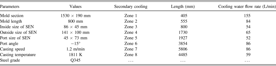
For numerical modeling of centerline segregation in a continuously cast slab, the computational domain includes the region from the meniscus to the solidification end, and the calculation cost increases exponentially with the number of grid points.Reference Li, Wu, Ludwig and Kharicha21 To decrease the amount of calculations and improve calculation efficiency, the computational domain is treated as follows. First, according to the previous nail shooting test,Reference Long, Chen, Wang, Luo, Han, Liu and Gao28 the strand in the present case solidifies completely in the secondary cooling zone 8. Thereby, the computational domain only includes the region from the meniscus to the end of secondary cooling zone 8. Second, a quarter symmetry strand computational domain is chosen to calculate in this study. Third, according to the flow characteristics of the molten steel in the liquid pool, the computational domain is reasonably divided into two parts: 3-D turbulent flow region and natural convection region. This is the most effective way to improve the calculation efficiency. The division method is illustrated in Fig. 1(a). In the turbulent flow region, the molten steel in the liquid pool exhibits reflux in the casting direction. The turbulent fluxion of the molten steel has a great impact on the solute distribution in the liquid pool. Hence, the flow states of the molten steel in three dimensions must be included in the coupling calculation of the flow, heat, and solute transport in the turbulent flow region. Thus, a 3-D coupling model of the flow, heat, and solute transport is applied in the turbulent flow region to investigate the transport phenomena during the CC process. However, when the z-component of velocity of the molten steel is equal to the casting speed, plug flow occurs in the liquid pool, and the local molten steel and shell exist in a relatively static state. Therefore, we deduce that there is no convection of the molten steel in the casting direction, meaning that the molten steel flow in the casting direction has no effect on the solute distribution. Therefore, a 2-D slicing model for the centerline segregation prediction can be applied to this natural convection region. In the 2-D slicing model, the natural convection (except the flow in the casting direction), the heat, and the solute transport in the transverse section are coupled. Based on the above analysis, we believe that the first transverse section where the z-component velocities are equal to the casting speed is the interface between the turbulent flow region and the natural convection region. The data of interface from the calculation of the 3-D turbulent flow region are transmitted to the initial 2-D slice applied in the natural convection region by a coordinate interpolation algorithm. Using such a process, the 3-D coupling model is combined with the 2-D slicing model to predict the centerline segregation during the slab CC process. The geometry and working parameters of the CC process are listed in Table I.
(a) Division of the computational domain for the simulation of the centerline segregation during the slab CC process, (b) meshes of the 3-D turbulent flow region, and (c) meshes of the 2-D natural convection region.

The geometry and working parameters of the slab CC process.

To determine the interface between the 3-D turbulent flow region and the 2-D natural convection region, a part of the computational domain (from the meniscus to the secondary cooling zone 4) was built and calculated. The position of this interface is obtained by analyzing the variation of z-component of the velocity of molten steel at the central symmetry plane of the strand narrow face. The meshes adopted for the 3-D turbulent flow region and the 2-D natural convection region, which were generated by ANSYS ICEM CFD 14.0, are shown in Figs. 1(b) and 1(c). The maximum size of the grid is 5 mm, which is sufficient to determine a precise solute distribution and centerline segregation profile.Reference Li, Wu, Ludwig and Kharicha21
C. Boundary conditions and physical properties
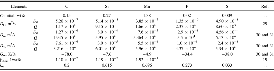
The inlet velocity of the submerged entry nozzle (SEN) was calculated based on the mass conservation. The K and ε were estimated using semi-empirical relations. The values of these parameters are v in = 1.502 m/s, k = 0.003 m2/s2, ε = 0.0134 m2/s3, and T = 1811 K. The initial concentrations of each solute elements (C-initial) listed in Table II are the mean values of 60 heats of steel Q345 from plant records.
Initial concentrations and species-dependent thermophysical properties.

A wall condition was used at the strand surface. The heat flux at the mold surface was calculated by Eq. (23),
 $${q_{\rm{m}}} = 2,680,000 - 276,000 \times \sqrt {{{60{L_{\rm{Z}}}} \over {{V_{\rm{c}}}}}} \quad .$$
In the secondary cooling zone, the heat transfer coefficient was calculated using Eq. (24). More details about the boundary conditions for heat transfer in the secondary cooling zone are available in our previous publications.Reference Long and Chen17,Reference Long, Dong, Chen, Liao and Ma18 In every cooling zone (cooling circuit), the integrated heat transfer coefficient was used.
 $$h = 2950.190 \times T_{\rm{w}}^{ - 0.235} \times {w^{0.805}}\quad .$$
The partition coefficient (k m) is a critical parameter for segregation simulation and modeling accuracy. It is highly dependent on the phase constitution of the mushy zone, the temperature, and the alloy components. Therefore, k m should be determined according to the initial concentrations in the steel (listed in Table II) by thermodynamic calculation prior to the macrosegregation simulation. Additional details on the thermodynamic calculation for k m in a multicomponent system are available in our previous publication.Reference Chen, Long, Cao, Chen, Liu and Dong26
Figure 2 shows the evolution of k m with the phase constitution of the mushy zone during the solidification process for steel Q345. Figure 2(a) indicates that the mushy zone of steel Q345 experiences three difference phase constitutions during solidification. First, as the temperature decreases to 1786 K (liquidus temperature), liquid phase (L) and ferrite (δ) coexist. In this coexistence region, the solutes redistribute between δ and L. As the solidification proceeding, the temperature of the system decreases and L transfers into δ, which results in an increase in the amount of δ. Second, when the temperature of the system falls below 1755 K, the peritectic reaction occurs. The L and δ phases transform into austenite (γ), meaning that the amount of L and δ decrease gradually, and the amount of γ from the peritectic reaction increases. In this region, where the temperature ranges from 1755 to 1753 K, three phases (L, δ, and γ) coexist, and the solutes redistribute among L, δ, and γ until exhausting the amount of δ. When the temperature of the system reaches 1753 K, the peritectic reaction terminates. Third, after the peritectic reaction, as the temperature of the system further decreases, L transforms into γ gradually until solidification is complete. In this region, where temperature ranges from 1753 to 1737 K, L and γ coexist, and solutes distribute between γ and L.
The evolution of equilibrium partition coefficients with solidification path during steel Q345 solidification: (a) solidification path and (b) equilibrium partition coefficient.

Figure 2(b) illustrates the evolution of k m during solidification of steel Q345. For the solute C, from 1786 to 1755 K, k C between δ and L remains almost constant at 0.148. From 1755 to 1753 K, the amount of γ generates from the peritectic reaction increases gradually. Over this temperature range, k C among δ, γ, and L increases rapidly as k C between γ and L, which is roughly twice of that between δ and L. From 1753 to 1737 K, k C between γ and L further increases as the temperature decreases. For the solute Si, k Si increases as the temperature decreases, although it experiences a slight reduction when the phase constitution of the mushy zone changes from δ and L to δ, γ, and L. In contrast to the solute Si, k Mn decreases with the temperature, but it experiences an increase in the three-phase (δ, γ, and L) coexistence region. The reason for this is that k Mn between γ and L is greater than that between δ and L. In addition, the values of k P and k S exhibit similar variation tendencies. First, k P and k S slightly increase as the temperature decreases and then experience a sharp reduction in the three-phase coexistence region. Finally, k P and k S further decrease with the temperature until solidifying completely.
According to the above analysis, it is evident that the effect of phase constitution on k m is significant. This effect was considered in the present study. However, due to the slight difference in the range of the mushy zone between the macrosegregation numerical model and the thermodynamic model during solidification, it can cause numerical errors and convergence difficulties when the evolution curves of k m are applied directly to the macrosegregation simulation. Instead, the mean values of k m for difference solutes (listed in Table II) over the entire mushy zone (from 1786 to 1737 K) were applied in the centerline segregation model.
The diffusion coefficients for different solutes were calculated using Eq. (25),
 $$D = {D_0} \cdot \exp \left( { - {Q \over {RT}}} \right)\quad ,$$
where the constants D 0 and Q are listed in Table II, T is the temperature, and R is the gas constant.
The other species-dependent thermophysical properties are listed in Table II.
The physical properties of steel Q345 used in the calculation are listed in Table III.
Physical properties of steel Q345.

D. Solution procedure
The centerline segregation simulation model was solved using the SIMPLE algorithms with ANSYS Fluent 14.0. The calculation was performed on a computer with a 3.50-GHz Intel core i7-4770k processor and 16.0-GB RAM. In the present simulation, the time step size was set at 0.05 s. The residuals of continuity, velocity components, solutes, and K were set 0.001, whereas the residual for ε was set at 1 × 10⁻⁶. For each time step, if the residual is less than the specified value, the particular equation is deemed to have converged.
E. Model validation
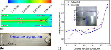
To verify the accuracy of the centerline segregation model, first, the solute distribution in the slab transverse section predicted by the present model was compared with the morphology of strand transverse section. Figure 3(a) shows the distribution of the solute C in the slab transverse section after complete solidification. The solute elements are rejected from the solid phase to the liquid phase during steel solidification. With the effect of molten steel convection, the solute elements are transported to the liquid pool, leading to the solute concentration of solutes in the liquid pool increasing as solidification proceeding. Finally, after complete solidification, the solute elements are found to enrich the centerline region of the slab transverse section. This centerline segregation morphology of the slab is indirectly in accordance with the segregation line exhibited in the morphology of the strand transverse section obtained by acid etching [shown in Fig. 3(b)]. Furthermore, as the results shown in Fig. 3(a), we found that the solutes enrich more seriously at the front-end of the triangle region. And this characteristic pattern is also detected in the morphology of the strand transverse section, as shown in Fig. 3(b). These comparisons demonstrate that the distribution pattern of solute C in the slab transverse section agrees with the morphology of the slab transverse section.
(a) The distribution of C predicted by the hybrid simulation model in half of the slab transverse section. (b) Morphology of the centerline segregation in half of the slab transverse section. (c) The comparison between the calculated and measured profiles of the solute C for 1/2 line (Y = 0 mm) of the strand.

To further verify the accuracy of the centerline segregation model, the chemical element C across the 1/2 line (Y = 0 mm) of the strand was evaluated using a carbon and sulfur analyzer (CS-8820, Wuxi Jiebo Electrical Technology Co., Ltd., Wuxi, China). Details regarding the location of the sample drillings and the test results are shown in Fig. 3(c). The diameter of the drill is 5 mm and the distance between two drilled holes is 15 mm. The results shown in Fig. 3(c) indicate that the segregation degree of C from the present numerical model of centerline segregation exhibits the same tendencies as the data from the experiment. From the slab surface to the slab center, the concentration of C increases gradually and reaches a maximum in the center. The calculated and experimental centerline segregation degrees of C are 1.135 and 1.15, respectively, corresponding to a deviation of 1.3%. Furthermore, the average deviation (taken using seven sampling points) between the calculated and experimented results reaches as low as 0.5%. The comparisons between the simulation and the experiment indicate that the results from the present simulation model feature relatively high reliability. Thus, the 3-D combined with the 2-D hybrid simulation model of centerline segregation was used for the subsequent numerical calculations. The characteristics of solute distribution in the entire strand and the macrosegregation profile in the transverse section of the slab during the CC process were obtained by numerical modeling using this hybrid model.
III. RESULTS AND DISCUSSION
A. Flow and solute transport in the turbulent flow region
To determine the interface between the turbulent flow and natural convection regions, the flow characteristics of molten steel in the turbulent flow region are discussed first. The flow pattern of molten steel in the turbulent flow region is shown in Fig. 4(a). The molten steel jet flows through the port of SEN, impacts the narrow face of the mold, and then is divided into two parts at the impact point and forms upper and lower recirculation vortices, which is useful to stabilize the slab CC process and improve molten steel purity. In the upper recirculation zone, the high-temperature fresh molten steel is brought to the meniscus and maintained at a relatively high temperature. It is very important to increase the mold powder melting rate. In the lower recirculation zone, the recirculation vortex is useful to promote the agglomeration of small-sized inclusions. Then, the relatively large-sized inclusions float up and are trapped by the mold powder flux. In addition, as the velocity vector in the different transverse sections shown, the convection of molten steel in the casting direction is significant. However, the convection intensity in the turbulent flow region gradually decreases with the increasing distance from the meniscus. Therefore, the convection of molten steel in the casting direction will cease at a certain position where the plug flow is formed.
(a) Flow in the turbulent flow region. (b) The z-component of velocity and velocity magnitude for a line 10 mm from the narrow face on the central symmetry plane. (c) The z-component of velocity for different lines on the central symmetry plane of the strand narrow face.

The variations in the z-component of velocity and the velocity magnitude at 10 mm from narrow face in the casting direction are shown in Fig. 4(b). At the impact point of the molten steel jet on the narrow face, the z-component of velocity of the jet is equal to zero, and the velocity magnitude reaches a valley. From the results shown in Fig. 4(b), we see that the impact point is located at a position approximately 438 mm below meniscus. Moreover, both the z-component of velocity and the velocity magnitude remain unchanged below a position 0.8 m from the meniscus. The reason for this is that the molten steel at this position (10 mm from the narrow face) has solidified completely and the velocity is equal to the casting speed (0.02 m/s).
The variations of the z-component of velocity for different characteristic lines on the central symmetry plane of strand narrow face are shown in Fig. 4(c). If the z-component of velocity is positive, the molten steel flows upward. Conversely, if the z-component of velocity is negative, the molten steel flows downward. As the distance from the meniscus increases, the z-component of velocity gradually tends to equal the casting speed. Below the end of the secondary cooling zone 3 (located 2560 mm below meniscus), the velocity of the molten steel at the central symmetry plane of the strand narrow face is equal to the casting speed, meaning that the plug flow has occurred, and there is no relative movement in the casting direction. Therefore, the transverse section at the end of the secondary cooling zone 3 is selected as the data transmission interface. The 2-D slicing segregation model is adopted over the natural convection region from the secondary cooling zone 4 to zone 8.
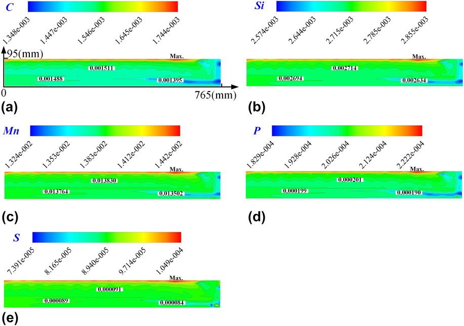
Figure 5 shows the liquid fraction and the distributions of different solutes at the data transmission interface. As the solidification profile shown in Fig. 5(a), the solidified shell is relatively uniform around the transverse section, with the exception of near the narrow face. This reflects that the effect of cooling water on the strand is relatively uniform. However, due to the impact of fresh molten steel, the solidified shell near the narrow face of the slab remelts. This is the reason that the solidified shell near the narrow face is slightly weaker than at the other position.
Solidification profile and solute distribution at the data transmission interface (2560 mm from the meniscus): (a) liquid fraction, (b) C, (c) Si, (d) Mn, (e) P, and (f) S.

The distributions of C, Si, Mn, P, and S are shown in Figs. 5(b)–5(f), indicating that these solutes have the same distribution. As mentioned, the solute distribution is closely related to the flow state of the molten steel in the liquid pool. In the turbulent flow region, the flow of molten steel in the turbulent flow region is intense, resulting in a uniform distribution of the solute elements in the liquid pool. In addition, the concentration of the solute near the slab surface is approximately equal to the initial concentration. The reason for this is that the solidified rate is very fast when the initial solidification shell starts to form in the water-cooled mold. Thus, the molten steel near the slab surface has already solidified completely, even as the solute elements have not completely diffused and transferred to the liquid pool. Moreover, from the element distribution on the slab transverse section, we see that all the solutes exhibit a negative segregation region near the narrow face. This is a result of the molten steel impacting and washing this region, and the solutes rejected from the solid phase were taken away and enrich the liquid pool. The data of the interface from 3-D coupled model, including the concentrations of all solute elements, temperatures, ε, k, x-component, and y-component of velocity, are treated as initial conditions and transmitted to the 2-D slicing model by a coordinate interpolation algorithm.
B. Evolution of solute segregation in casting direction
The evolutions of solute segregation for different characteristic lines on the central symmetry plane of the strand narrow face along the casting direction are shown in Fig. 6. As the results shown in Fig. 6(a), all the distributions of solutes at the slab center along the casting direction (Y = 0) exhibit the same tendency. When the steel in the slab center is in a liquid state (solid fraction equal to 0), solute concentrations keep increasing along the casting direction. The reason for this is that the solute elements are rejected from the solid phase to liquid phase, and as solidification proceeding, the concentration of solute elements enriched in the liquid pool continues to increase. When the steel in the slab center enters the mushy state (solid fraction between 0 and 1), the solute concentration further increases, although the rate begins to taper off. During the later stages of solidification, the increasing rate of C is greater than that of S because the diffusion rate of C is greater than S. After solidifying (solid fraction equaling to 1), the solute concentration maintains a roughly constant value. This is a result of there being no solute elements rejected after complete solidification and that the diffusion rate of solutes in the solid phase is very slow. Moreover, the central segregation degree of the solute elements can be obtained after complete solidification. As the results shown in Fig. 6(a), the central segregation degree of the solutes C, Si, Mn, P, and S at the slab center (Y = 0 mm) are 1.135, 1.046, 1.036, 1.088, and 1.133, respectively. Thus, the segregation degree of the solutes is strongly related to the equilibrium partition coefficient of solutes. In general, the greater the partition coefficient is, the higher the segregation degree will be.
The evolution of the solutes as a function of solid fraction on different lines on the central symmetry plane of the strand narrow face in the casting direction: (a) Y = 0 mm, (b) Y = 191 mm, (c) Y = 382 mm, and (d) Y = 574 mm.
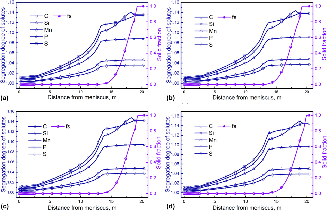
The results for the other three different characteristic lines (Y = 191 mm, 382 mm, and 574 mm) are shown in Figs. 6(b)–6(d), indicating that the evolution profile of solute segregation in the casting direction is the same as in Fig. 6(a). However, by comparing the results in Figs. 6(a)–6(d), we see that the central segregation degree of the same solute element at different positions (Y = 0 mm, 191 mm, 382 mm, and 574 mm) exhibits a slight difference. The central segregation degrees of the solute C at different positions (Y = 0 mm, 191 mm, 382 mm, and 574 mm, in turn) are 1.135, 1.139, 1.143, and 1.145, respectively. Similarly, the central segregation degrees of the solute Si are 1.046, 1.047, 1.047, and 1.050, respectively. The central segregation degrees of the solute Mn are 1.036, 1.037, 1.038, and 1.039, respectively. The central segregation degrees of the solute P are 1.088, 1.091, 1.094, and 1.097, respectively. Finally, the central segregation degrees of the solute S are 1.133, 1.138, 1.142, and 1.146, respectively. It is obvious that the central segregation degree of the solutes is related to the position on the centerline. Among these four specific positions, the central segregation degree of the solutes is most severe at the position Y = 574 mm, followed by Y = 382 mm, 190 mm, and 0 mm in sequence.
Furthermore, from the evolution of the solid fraction in the casting direction shown in Figs. 6(a)–6(d), the length of the liquid pool (the distance from the meniscus to the point where the solid fraction first equal 1) at different positions (Y = 0 mm, 191 mm, 382 mm, and 574 mm) exhibits slight differences. The lengths of the liquid pools at different positions (Y = 0 mm, 191 mm, 382 mm, and 574 mm, in turn) are 19.26 m, 19.26 m, 19.36 m, and 19.36 m, respectively. From this, it appears that the liquid pools’ lengths are in accordance with the central segregation degree of solutes. Thus, the central segregation degree at the centerline is closely related to the order of solidification. Among these four specific locations, the molten steel at the position Y = 574 mm is the final position to completely solidify, leading to the central segregation degree of the solutes at this position being more severe than at the other three positions.
C. Centerline segregation in the slab
The profiles of centerline segregation for different solutes on the slab transverse section are shown in Fig. 7, indicating that the solutes C, Si, Mn, P, and S exhibit the same distribution in the transverse section. From this, we see that these solutes are rejected from the solid phase to the liquid phase during solidification of the steel. Under the action of solute diffusion and the relative movement of the molten steel, the solutes enrich the liquid pool, leading to the concentration of solutes in the liquid pool increasing as the solidification proceeding. Finally, serious central segregation occurs at the centerline of the slab transverse section after solidifying completely. In addition, as discussed in Sec. III.A, an obvious negative segregation region (shown in blue) exists near the narrow face. This negative segregation is a result from the washing action of the molten steel in the turbulent flow region and is inherited from formation to complete solidification of the strand. At the approximate position Y = 614 mm, the solute concentration is the highest. The reason for this is that final complete solidification of the molten steel occurs at this position.
The profiles of centerline segregation for different solutes in the slab transverse section (quarter): (a) C, (b) Si, (c) Mn, (d) P, and (e) S.

The evolutions of the segregation degree for different solutes on the 1/2 line (Y = 0 mm) are shown in Fig. 8(a), indicating that the concentrations of all these solutes increase from the slab surface to the center and reach a peak in the center. The segregation degree of the solutes C, Si, Mn, P, and S at the slab center are 1.135, 1.046, 1.036, 1.088, and 1.133, respectively. The segregation degree of S is higher than solutes Si, Mn, and P due to its lower equilibrium partition coefficient. However, comparing solutes C and S, their segregation degrees roughly maintain the same lever. This is because the diffusion rate of solute C is faster than solute S.
(a) The evolution of different solutes for the 1/2 line (Y = 0 mm) of the strand and (b) the evolution of different solutes for the centerline (X = 95 mm).

The evolutions of the central segregation degree for different solutes at the centerline are shown in Fig. 8(b). All solutes exhibit the same profile. With the exception of a narrow region of negative segregation near the narrow face of the slab, which is caused by the washing action of molten steel, all the solutes exhibit positive segregation on the centerline. Moreover, on the centerline of the slab, the maximum segregation degree is located at the position Y = 614 mm. The maximum segregation degrees of the solutes C, Si, Mn, P, and S are 1.163, 1.058, 1.045, 1.111, and 1.165, respectively. The segregation tendencies of C and S are the strongest, whereas Si and Mn are weak.
IV. CONCLUSIONS
To investigate and predict centerline segregation during slab CC, a combined 3-D and 2-D hybrid simulation model with a high calculation efficiency was developed. The large amount of calculations was decreased, and the calculation efficiency was improved by reasonably dividing the computational domain of the slab into a turbulent region and a natural convection region. The main conclusions are summarized as follows:
(1) The hybrid simulation model for the prediction of centerline segregation shows relatively high reliability. The average deviation between the calculated and experimental results reaches as low as 0.5%.
(2) The impact point of the molten steel on the narrow face is located at a position approximately 438 mm below the meniscus. The transverse section at the end of the secondary cooling zone 3 (2560 mm below the meniscus) is selected as the data transmission interface for the hybrid simulation model.
(3) In the casting direction, the concentration of solutes in the liquid pool increases gradually. From the liquid phase to the mushy zone, the increasing rate of solute concentration slows down. After solidifying completely, the solute concentration maintains an almost constant value.
(4) Macrosegregation occurring during slab CC processes has heredity. The negative segregation near the slab narrow face, caused by the washing action of the molten steel in the turbulent flow region, is inherited from formation to the complete solidification of the strand.
(5) The pattern of centerline segregation and solute distribution during slab CC were accurately predicted. The maximum centerline segregation degrees of the solutes C, Si, Mn, P, and S are 1.163, 1.058, 1.045, 1.111, and 1.165, respectively.
NOMENCLATURE

ACKNOWLEDGMENT
The authors would like to thank the Natural Science Foundation of China (NSFC) for the financial support (Project Nos. 51374260, 51504048, and 51611130062).