2.1 CFD solver

The CFD solver used in this research is three-dimensional multi-block structured finite volume solver (ADflow). This parallel implicit solver is capable of solving the Euler and Reynolds averaged Navier-Stokes (RANS) equations (steady and unsteady) [Reference van der Weide, Kalitzin, Schluter and Alonso19]. The discretisation of the governing equations is done by a finite volume approach with a central formulation over structured meshes. The convective terms are computed by the Jameson-Schmidt-Turkel [Reference Jameson, Schmidt and Turkel20] scheme using flux splitting upwind scheme with Van-Albeda limiter. Viscous fluxes are computed to second order accuracy using a central difference approach. The residual smoothing is made by employing an explicit 5th order Runge-Kutta algorithm employing well known steady-state acceleration techniques including local time stepping, and geometric multigrid. For RANS analysis the turbulent equations are solved in coupled fashion using diagonally dominant alternating direction implicit (DD-ADI) scheme. In order to improve convergence, the solver is also equipped with a diagonalised ADI method for the mean flow equations and Newton-Krylov (NK) solver. The computational coordinates are x, y and z axes, while x in the stream-wise direction, y vertical, and z span-wise. The origin is located at the wing leading edge.

2.2 Free Form Deformation (FFD) and mesh warping

The geometry parametrisation is done by the FFD approach [Reference Kenway, Kennedy and Martines21]. In this approach the geometry is located inside a B-Spline control volume while the coordinates are mapped to the external surface of the volume by a Newton search algorithm. All the geometric modifications are made on the external surfaces of the FFD volume. Any modification of the FFD boundaries indirectly modifies the internal geometry. The main assumption of this approach is a constant topology throughout the optimisation process. The mesh is warped in order to solve the flow field for the modified configuration. In this work the algebraic mesh perturbation scheme is used, which is developed by Kenway et al. [Reference Kenway, Kennedy and Martines21].

2.3 Optimisation algorithm

In this research work the SLSQP optimisation algorithm is applied. It is part of the pyOptSparse framework Perez [Reference Wu, Kenway, Mader, Jasa and Martines22], which is an open-source software. SLSQP is a sequential least square programming algorithm [Reference Kraft23] that evolved from the least squares solver [Reference Lawson and Hanson8]. It uses a quasi-Newton Hessian approximation and an L1-test function in the line search algorithm.

3.1 Baseline geometry

The initial geometry for this optimisation is the wing-body-tail configuration, also known as the drag prediction workshop (DPW) geometry [Reference Gaetan and Joaquim24], with the tail rotation set to zero. In the following cases, the optimisation will be run at a Reynolds number of $5 \times {10^6}$, which is the wind tunnel test configuration. The flight Reynolds number is 43 million calculated at the nominal cruise altitude of 37,000 feet and a Mach number of 0.85.

All coordinates are scaled by the mean aerodynamic chord (7.00532m, 275.8 in). The resulting reference chord is 1.0, and the half span is 4.194213. The reference area is 3.90961 (191.844777m2). The moment reference point is located at $\left( {x,y,z} \right) = \left( {4.80756,\;0.64525,\;0.0} \right).$ The nominal flight condition is a cruise Mach number of $M = 0.85$ with lift coefficient of$\;{C_l} = 0.5$.

3.2 Grid convergence study

A grid convergence study has been conducted based on the Grid Convergence Index (GCI) method, for examining the spatial convergence of CFD simulations presented in the book by Roache [Reference Roache, Ghia and While25]. Roache suggests a GCI can be used to provide a consistent manner in reporting the results of grid convergence studies and also an error band on the grid convergence of the solution. This approach is also based upon a grid refinement estimator derived from the theory of Richardson Extrapolation [Reference Anderson, Tannehill and Pletcher7]. The GCI for the fine grid is defined as: $GC{I_{fine}} = \frac{{{F_s}}}{{{r^p} - 1}}$ where ${F_s}$ is a factor of safety (recommended to be ${F_s} = 1.25$ for comparisons over three or more grids). The GCI for the coarser grid is defined as $GC{I_{fine}} = \frac{{{F_s}{r^p}}}{{{r^p} - 1}}$, while each grid level yield solutions that are in the asymptotic range of convergence for the computed solution. The parameter p is the order of convergence (here a second order accuracy is involved, so theoretically the maximum value is p = 2), and r is the effective grid ratio: $r = {\left( {{{{N_1}} \over {{N_2}}}} \right)^{\!\!\!{\raise0.5ex\hbox{$\scriptstyle 1$}\kern-0.1em/\kern-0.15em\lower0.25ex\hbox{$\scriptstyle d$}}}}$ where N is the total number of grid points in executive grid levels, and d is the flow dimension. The asymptotic range of convergence can be checked by observing the two GCI values as computed over three grids, $GC{I_{23}} = {r^p}GC{I_{12}}$, while values approximately unity indicates that the solution are within the asymptotic range of convergence.

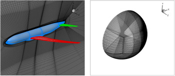
A structured multi-block mesh with a total number of 60 blocks is constructed by using ANSYS ICEM-CFD commercial software. The mesh convergence study is performed by three levels of grid refinement in order to assess the effect on the numerical accuracy, while the results of each grid level are summarised in Table 1. The grids (see Fig. 1) were generated with clustering cells near the walls that result in a range of ${y^ + } \approx 1 - 6$ at all the computed angle of attack. In this grid convergence study, a non-integer of grid coarsening is used since halving the grid may put the solution out of the asymptotic range. The same grid generation parameters were maintained as the original coarse grid.

Table 1.

Results of the mesh convergence study for the CRM wing-body-tail configuration

Figure 1.

Structured mesh (Level L0) generated by using ICEM-CFD commercial software. Left: Mesh on the symmetry plane and walls. Right: Farfield mesh.

The GCI values including the asymptotic range of convergence and an estimation of the aerodynamic coefficient values at zero grid spacing are detailed in Table 1, computed at $\alpha = {0^\circ }.$ Based on this study we can say that ${C_d}$ is estimated to be $0.026163\;$with an error band of 1.38%. The grid resolution studies confirmed that the computed aerodynamic lift coefficient, ${C_l}$, is grid converged (Table 1).

3.3 Optimisation problem formulation

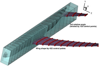
The objective is to minimise the drag subject to constant lift constraint$\;{C_l} = 0.5$. The wing-body-tail configuration is enveloped within 15 FFD blocks while the wing and the tail contain one block each. The design variables (listed in Table 2) are the y-coordinates of the 432 control points of the FFD blocks enveloping the wing and 120 control points enveloping the tail, as well as the angle-of-attack and the horizontal tail angle. The wing control points are not distributed uniformly since the performance of the wing in transonic conditions is highly effected by the leading edge shape. The FFD volume includes 24 points in the chordwise direction and 18 spanwise design sections (see Fig. 2). The geometric constraints (listed in Table 3) include thickness constraints, which are controlled by 1,000 control points distributed at 25 chordwise and 40 spanwise sections of the wing. The thicknesses are enforced to be no less than the thickness of the baseline geometry. The wing volume is constrained to be no less than the baseline configuration. Since the performance is sensitive to the leading and trailing edge shapes, a geometric constraint is added in order to control the geometry and avoid warping failure (see LE and TE in Table 3). All the cases that have been examined in this research work are summarised in Table 4, where$\;{C_l}$, ${C_m}$ are the lift and moment coefficient.

Table 2.

Design variables

Table 3.

Constraints

Figure 2.

The free-form deformation blocks envelope the wing-body-tail configuration. The design variables are defined on the wing and tail.

Table 4.

Cases calculated in this research work for drag minimisation

The flow converge to a density residual of ${10^{ - 8}}$ and the adjoint equation convergence was set also to ${10^{ - 8}}$. The optimality convergence tolerance of SLSQP optimisation algorithm was set to ${10^{ - 6}}$. The initial design point for all the optimisations is the baseline geometry, unless stated otherwise. The optimisations are performed using an eight-core 3.5GHz Intel processors pc with 32GB RAM.

3.4 Surface sensitivity of the baseline geometry

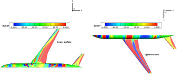
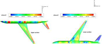
In order to examine the sensitivities of the baseline geometry, a sensitivity analysis of the drag and pitching moment is performed. The sensitivity of the drag and pitch moment coefficients with respect to the wing shape can be visualised through a sensitivity contour plots, shown in Fig. 3-Fig. 4. The derivatives of ${C_d}$ and ${C_{mz}}$ are plotted with respect to shape variations in the z direction. The highest gradient of ${C_d}$ is obtained in the shock regions on the upper wing surface. This indicates that shock reduction through local shape changes is the major driver in reducing$\;Cd$, and the optimisation algorithm will try to eliminate the shock and reduce the wave drag, at the first design iterations. As for $Cmz$, a high positive derivative is observed in the aft of the tail upper surface, indicating that moving the aft portion of the tail in the positive direction (y axis, trailing edge up) increases $Cmz$, resulting in a pitch-up movement. It is important to note here that these sensitivity plots are only a linearisation about the current design point and they provide no information about the constraints.

Figure 3.

Drag coefficient sensitivity analysis contour plots. Left: lower surface. Right: upper surface.

Figure 4.

Pitch moment sensitivity analysis contour plots. Left: upper surface. Right: lower surface.

3.5 Untrimmed wing aerodynamic shape optimisation

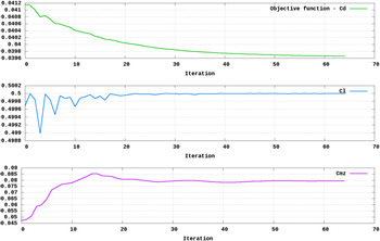
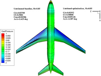
In this first study the results of the aerodynamic shape design optimisation of the CRM wing-body-tail configuration are presented with no enforcement of a trim constraint. The design variables are the 432 shape control points on the wing and the angle-of-attack, while the tail rotation is not a design variable in this case. Only lift and geometry constraints are imposed, therefore, one flow solution and three adjoint solutions (lift, drag and pitch moment) are needed at each design iteration. In order to examine the effect of the mesh level on the optimisation procedure, this study repeated three times for three mesh levels. The final results are listed in Table 5. Convergence is reached within 23.4 hours using 4 processors (for mesh level L0), with 47 calls to the objective function and 24 calls to the sensitivity analysis function. The convergence history of the aerodynamic coefficients (mesh L0) is shown in Fig. 5 for the three-level optimisation process. The optimised wing has a 5.76% lower drag than the baseline configuration. The drag coefficient decreased by 15.6 counts, from ${C_d} = 0.02708$ $to\;{C_d} = 0.02552$, with L0 mesh level. 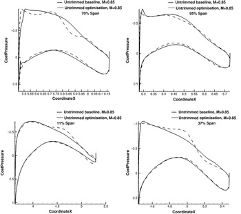The angle-of-attack slightly decreased from ${2.425^o}$ to$\;{2.387^o}$. The pitch moment coefficient increased from 0.01506 to 0.0512. Figure 6 shows a comparison of the optimised and baseline wing (mirrored view), with the pressure coefficient distribution on the wing’s upper surface. The pressure coefficient distribution at four sectional regions along the span are also shown in Fig. 7-Fig. 8, including the thickness and lift distribution. It is clearly seen that the shape design variables make a significant contribution to minimise the drag. The initial geometry exhibits a front of very closely spaced pressure contour lines spanning a significant portion of the wing, indicating a shock. The optimised wing shows parallel pressure contour lines with roughly equal spacing, indicating a nearly shock-free solution. This observation is confirmed by the sectional pressure distribution (see Fig. 7), mainly in 37% and 70% wing span, with smooth pressure variation along the wing chord compared to the initial design. The sharp increase in the local pressure due to the shock becomes a gradual change from the leading edge to the trailing edge.

Table 5.

Mesh convergence study for the untrimmed-shape optimisation case

Figure 5.

Convergence history of the aerodynamic coefficients for the untrimmed-shaped optimisation. The mesh level is L2 (coarse).

Figure 6.

Comparison of the untrimmed optimised shape pressure contours with the baseline configuration. The mesh level is L0 (fine).

Figure 7.

Comparison of the untrimmed-shaped optimisation with the baseline configuration. Shown is the pressure coefficient distribution in four sections along the wing’s span.

Figure 8.

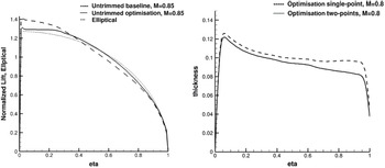
Comparison of the untrimmed-shaped optimisation with the baseline configuration for the wing thickness distribution (left) and the normalised lift (right). The parameter eta presents the normalised spanwise location.

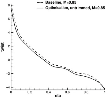
The optimised lift distribution is much closer to the optimal elliptical lift distribution, which is shown by the dotted line. The thickness and volume of the optimised wing is about 1% lower on average compared to the initial design, although a geometric constraints are imposed. This thickness reduction probably contributes to the wave drag reduction. Although twist was not defined as a design variable, the actual optimised wing obtained is more twisted than the baseline configuration as it is clearly demonstrated in Fig. 9. The movement of the shape design variables fine-tuned the twist distribution. The optimised design has more twist along the span except the root and the tip, and the overall twist angle is the same: around 11.5 degree. This twisting mechanism is the main driver for the shock elimination on the wing’s upper surface.

Figure 9.

Comparison of the untrimmed-shaped optimisation with the baseline configuration for the wing twist distribution.

Since no trim condition is imposed, the pitch moment coefficient is increased by more than 70%. From this study we can learn that optimising the wing with no trim condition by tail rotation results in shock-free design with a considerably improved drag. From the excessive pitch moment obtained we can expect to have an increased drag in a trimmed configuration. We also expect the angle-of-attack to increase in trimmed optimised configuration in order to compensate the lift loss obtained by rotating the tail. However, since most of the drag is obtained by the body and the tail, the angle-of-attack variation has a large and wider effect, related to the integral drag value. Therefore, the optimisation algorithm “prefers” to slightly modify the wing shape instead of varying the angle-of-attack. This issue is discussed in the following section.

It is important to mention here that the variation in the drag coefficient between the baseline and the optimised meshes is not totally constant, and this fact did not give the author the confidence that the optimisation using the coarse meshes represent the design space sufficiently well. Therefore, the optimisation studies were performed on the three mesh levels in order to carefully footprints the mesh effect on the optimised configuration. However, since the author is looking at this optimisation problem from an industrial point of view, the main focus here is on the delta values between the baseline and the optimised configurations, and not the absolute objective value itself. After all, the corrected design trends were captured even with the coarsest mesh.

3.6 Aerodynamic shape optimisation of the wing with Trim constraint

In this study the effect of the trim constraint by the tail rotation is investigated. The formulation is the same as that of the previous study with the addition of the tail rotation angle as a design variable (in addition to the 432 shape control points on the wing and the angleof-attack). Lift, pitch moment and geometry constraints are imposed; therefore, one flow solution and four adjoint solutions are needed at each design iteration. In order to examine the effect of the mesh level on the optimisation procedure, this study repeated three times for three mesh levels. The final results are listed in Table 6.

Table 6.

Mesh convergence study for the trimmed-optimised configuration

Convergence is reached within 63.75 hours using 4 processors (for mesh level L0), with 81 calls to the objective function and 71 calls to the sensitivity analysis function. The convergence history of the aerodynamic coefficients is shown in Table 6 for the three-level optimisation process. The optimised wing has 6.76% lower drag than the baseline configuration. The drag coefficient decreased in 16.7 counts, from ${C_d} = 0.02708$ to$\;{C_d} = 0.02541$, for the L0 mesh level, which is 1.1 lower than the untrimmed-optimised wing. Although one would expect an increased angle-of-attack in order to compensate the negative lift obtained on the tail required to trim the configuration, there is no significant change observed in the angle-of-attack. The lift and pitch moment constraints are satisfied, and the geometric constraints (namely volume and thickness of the wing) are not satisfied to the tolerance of ${10^{ - 6}}$ pre-defined within the optimisation algorithm.

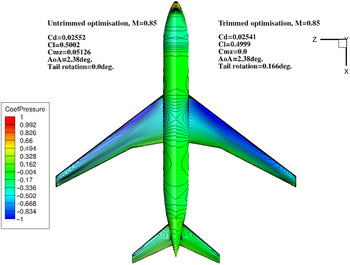
Figure 10 shows a comparison of the trimmed-optimised and untrimmed-optimised wing, with the pressure coefficient distribution on the wing’s upper surface. It is also shown the thickness and lift distribution (Fig. 11). It is clearly seen that the shape design variables make a significant contribution to minimise the drag. The surface pressure distribution is similar to the untrimmed-optimised case.

Figure 10.

Comparison of the trimmed-optimised wing pressure contours with the untrimmed-optimised configuration.

Figure 11.

Comparison of the trimmed-optimised wing with the untrimmed-optimised configuration for the normalised lift distribution (right) and wing thickness (left).

The trimmed-optimised lift distribution is not close to the optimal elliptical lift distribution (shown in dotted line), compared to the untrimmed-optimised wing. The volume and thickness constraints are not satisfied, while the volume of the optimised wing is about 4.7% lower on average compared to the initial design (see Fig. 11, for mesh level L0), although a geometric constraints are imposed. This fact is one of two possible reasons for the improved drag reduction obtained with the trimmed-optimised wing compared to the untrimmed-optimised case. It is important to mention that the volume constraint is not satisfied with all the mesh levels, while the final scaled wing volume is about 0.96 times the baseline design.

From this study we can learn that optimising the wing with a trim condition by tail rotation results in shock-free design with a considerably improved drag, even better than the untrimmed-optimised case. First, since the trim condition results in an increased negative lift on the tail, which is actually rotated with leading edge downward, the induced drag generated by the tail is reduced. Second, the final trimmed-optimised wing is thinner than the baseline configuration (since the volume constraint is not satisfied) and this fact directly affects the wing drag performance. In addition, although we expected the angle-of-attack to increase in a trimmed-optimised configuration in order to compensate the lift loss obtained by rotating the tail, actually the angle-of-attack is not increased at all. The angle-of attack-variation has a large and wide effect integral drag value. Therefore, the optimisation algorithm “prefers” to slightly modify the wing shape instead of varying the angle-of-attack, and in this way an even higher drag reduction is obtained.

3.7 Trimming the baseline configuration

In this section the effect of the wing baseline configuration trim constraint is investigated with no-shape design. This study is valuable and important for the case of aerodynamic optimisation of the wing that includes trimming by rotating the tail, which is presented in the next section. Trimming the baseline configuration with no-shape optimisation can give us the rotation angle (and angle-of-attack) needed to achieve the trim, and the amount of drag penalty that we pay for this constraint.

The formulation is the same as that of the previous study, with the addition of trim constraint and no-shape optimisation. The design variables are the angle-of-attack and the tail rotation angle. Only lift and pitch moment constraints are imposed; therefore, one flow solution and two adjoint solutions are needed at each design iteration. In order to examine the effect of the mesh level on the optimisation procedure, this study repeated three times for three mesh levels. The final results are listed in Table 7.

Table 7.

Mesh convergence study for the trimmed baseline configuration

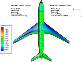
The trimming condition obtained at ${0.27^\circ }$ tail rotation angle (see Fig. 12, for mesh level L0) and nearly no drag reduction was obtained. The angle-of-attack slightly increased from ${2.425^\circ }$ to ${2.454^\circ }$.

Figure 12.

Comparison of the untrimmed baseline wing pressure contours with the trimmed-optimised wing.

3.8 Trimming of the aerodynamic untrimmed-optimised wing configuration

To achieve a reasonable comparison for the optimisation studies and to examine the off-design trimmed-optimised wing results, an optimisation calculation of the optimised untrimmed configuration is performed with the design variables set as the angle-of-attack and tail rotation angle only. Namely, the untrimmed-optimised wing geometry is analysed without modifying the wing but only to reach the trim condition by rotating the tail and varying the angle-of-attack.

In this case no constraints are imposed, therefore, one flow solution and two adjoint solutions are needed at each design iteration. Convergence is reached within 2.08 hours using 4 processors (for mesh level L0). The optimised wing has 1.54% higher drag than the untrimmed-optimised configuration. The drag coefficient increased by 4 counts, from $Cd = 0.0552$ to$\;Cd = 0.02592$. The optimised tail rotation angle for the trimmed optimisation increased to$\;{0.868^\circ }$, compared to ${0.166^\circ }$ of the trimmed-optimised wing. The angle-of-attack also increased from ${2.38^\circ }$ to ${2.48^\circ }$ for the optimised wing.

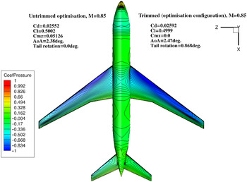
Figure 13 shows a comparison of the trim-optimised and untrimmed-optimised wings, with the pressure coefficient distribution on the wing’s upper surface. It is clearly seen that the trimmed wing shows a higher pressure jump near the wing tip region indicating a shock. From this study we can learn that the increased drag is primarily due to the increased tail rotation angle, and since the wing shape does not change, the trim drag is relatively insensitive to the angle-of-attack.

Figure 13.

Comparison of the untrimmed-optimised configuration surface pressure distrinution with the case of trimming the untrimmed-optimised wing configuration. The mesh level is L0 (fine).

4.1 Baseline geometry and grid convergence study

The wing geometry parameters are scaled by the root aerodynamic chord, C, and the origin is located at the root leading edge. Moment’s reference point is (0.3, 0, 0). The reference area for the aerodynamic force coefficients calculations is ${S_{ref}} = 0.786$ squared reference units. The wing half span is $L = 3.289$ reference units.

For the grid convergence study three structured hyperbolic volume O-meshes were generated by using pyHyp routine [Reference Secco, Kenway, He, Mader and Martins26]. The initial surface mesh is generated by using the commercial ICEMCFD software. The farfield is located at 50L. The coarse grid (level L2) is refined in three directions by a factor of 1.5, and the aerodynamic coefficients and baseline grid size are listed in Table 8. The grids are generated with clustering of cells near the walls, which results in a maximum of ${y^ + } \approx 15$, for the coarsest mesh level L2. The grid convergence study was made based on the GCI method, for examining the spatial convergence of CFD simulations presented in the book by Roache [Reference Roache, Ghia and While25]. The GCI values including the asymptotic range of convergence and an estimation of the drag coefficient at zero grid spacing is detailed in Table 8, computed at $\alpha = {5.7^\circ }.$ Based on this study we can say that ${C_d}$ is estimated to be ${C_d} = 0.145826414$ with an error band of 0.0492%. The grid resolution studies confirmed that the computed drag coefficient is grid converged.

Table 8.

Grid convergence study parameters for the gliding configuration wing

It is clearly seen that fine mesh analysis shows that there is some benefit to make an optimisation on a finer mesh. However, since the aerodynamic shape optimisation study is done for an industrial application, and in industry there are inflexible time limitations and limited computational resources, the subsequent single-point, multi-point and trimmed configuration problems are conducted using the medium mesh (Level L1).

4.2 Optimisation problem formulation

Several FFD frames are generated and examined in different topologies. The FFD is fitted very close to the wing surface to allow for better control on the warping procedure. In order to improve the convergence behaviour, the control points are spatially equally set up close to the surface. The control points used are the y-coordinates normal movements of 176 control points on the FFD frame: 22 chordwise and 8 stations in the spanwise direction (see Table 9). The angle-of-attack is also included in the design variables. The root trailing and leading edges control points are fixed in order to not permit any twist. In order to avoid warping failures, the leading and trailing edge control points are allowed to move in the same direction. The design variables include the twist of sections along the span about an axis located at 30% of the wing root chord. Twist is performed by allowing the y-coordinates of the FFD control points to vary and shear the wing’s sections. The twist at the root is not allowed.

Table 9.

List of design variables used for the wing aerodynamic shape optimisation

The thickness is controlled by 176 control points in the same order and is set to be no less than 75% of the baseline thickness at each control point, for spanwise sections higher than 30% of the span (outboard of the wing), and no less than the baseline thickness at in inboard of the wing. A list of the control points and constraints are presented in Table 10.

Table 10.

List of constraints for the optimisation of the wing

4.3 Single-point optimisation in transonic flow

The problem is the drag minimisation of the wing by optimising the shape and twist at a lift constraint in the following conditions: $Cl = 1.52$, $M = 0.8$ and$\;Rey = 2.66 \times {10^6}$. The optimisation is conducted with mesh L1. The solution process is started with the DDADI method until the total residual norm is reduced by five orders of magnitude. Then the solver is switched to ANK for better performance. The relatively selected lower convergence level (${10^{ - 5}}$) for the switch between the solvers improves the robustness of the nonlinear solver, although it comes at the cost of sub-optimal performance for simpler cases. The optimality convergence condition in SLSQP is set to ${10^{ - 6}}$, and the optimiser successfully reached the optimality tolerance defined.

Since the baseline configuration has a nearly constant thickness values along the wing span, it directly influences the overall convergence “behaviour,” and the optimisation convergence is less challenging than the CRM case. That is to say, the nearly constant thickness variation and the fact that the baseline wing is not twisted, makes the wing to be less sensitive to the mesh warping procedure. The lower and upper bounds of the y-coordinate control points are defined to move in the range of $ \pm 0.005$ reference units. For this purpose, the wing is divided to 8 spanwise sections, with each section consisting of 22 chordwise points (the trailing edge control points are fixed).

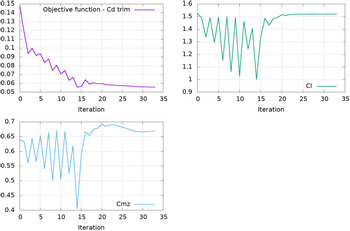
The objective function ${C_d}$, lift and pitch moment coefficients histories are presented in Fig. 14. The optimisation process decreased the drag coefficient from 1,475 counts to 550 counts, namely 925 counts, which is a reduction of 62.7%, within 45 design iterations.

Figure 14.

Drag, lift and pitch moment coefficients convergence histories for the single-point optimisation of the transonic wing configuration.

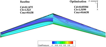
The pressure coefficient distribution on the upper surface for both the baseline and optimised wing is shown in Fig. 15. One can see the appearance of shock waves generated on the baseline wing, while for the optimised wing these shocks are eliminated. This effect is also demonstrated by the equally spaced pressure contour lines, which indicates a shock free solution.

Figure 15.

A comparison (mirrored view) of the pressure coefficient distribution on the upper surface of the baseline (left) and optimised transonic wing configuration (right). The results obtained with mesh level L1.

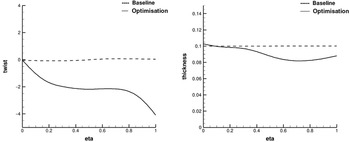
The thickness distribution obtained in the optimised wing is different than the baseline wing (see Fig. 16). The optimisation algorithm allows thickness reduction of nearly 25%, the lower bound of the thickness constraint. The drag reduction is achieved mainly by fine-tuning the twist distribution. The baseline wing is not twisted, while the optimised design is twisted from the root to the tip, with a nearly constant twist angle of 3.5 degree near the mid-wing, whereas the overall twist angle at the tip is nearly 5 degrees. The twist variables also provide a way for the optimiser algorithm to minimise the induced drag by modifying the spanwise lift distribution.

Figure 16.

Twist (left) and thickness (right) distribution along the wing span. A comparison between the baseline and optimised geometry.

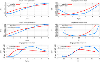
Figure 17 shows the drag polar for the optimised wing compared to the baseline wing configuration. The drag polar shows that the drag reduction relative to the baseline curve improves at an increased Cl. The aerodynamic efficiency improvement (Cl/Cd) is marginal for $\alpha = {3^\circ }$, $Cl = 1.25$. It is clearly seen that at negative angles of attack the wing performance are damaged (since a high lift coefficient as constraint, is involved). At positive angles of attack there is a significant advantage to the optimised wing over the baseline configuration, in terms of manoeuvering capabilities and aerodynamic efficiency (gliding distance).

Figure 17.

Polar graphs generated by the optimised geometry and compared to the baseline wing configuration.

4.4 Single-point optimisation in subsonic flow

The main challenge of the previous transonic optimisation case ($M = 0.8$) was to minimise the wave drag generated by the shock waves while satisfying the minimum thickness constraint and lift constraint. In the following optimisation case the drag is minimised for $M = 0.6$ with the same setup of design variables while the lift constraint is now $Cl = 2.127$ and the Reynolds number is $1.3 \times {10^6}$.

After 56 design iterations, a converged optimisation result has been achieved. The optimisation procedure reduced the drag coefficient from 1,225 counts to 796 counts, the drag is reduced by 35%. The lift and thickness constraints are satisfied within less than 10 design iterations by increasing outboard twist and reducing the angle-of-attack to ${7.2^\circ }$.

4.5 Multi-point aerodynamic shape optimisation

The single-point design is relatively robust to flight conditions, but further robustness is achieved through a multi-point optimisation. The single-point optimised wing resulted in a thin outboard of the wing, which was caused mainly by the thickness constraint (25% of the baseline). There are two disadvantages for thin wing with sharp leading edge. First, it is prone to flow separation in off-design conditions. Second, the thinner wing probably weights higher, when structural design is considered. So this issue is addressed by multi-point optimisation.

The problem formulation includes two operating points with variable Cl and M, summarised as follows: C1: $Cl = 1.52,\;M = 0.8$, C2: $Cl = 0.48,\;M = 0.55$. The objective function is defined as the weighted average drag (0.5). We consider an optimisation run converged when the residual of the first order optimality conditions drops below a tolerance of ${10^{ - 6}}$.

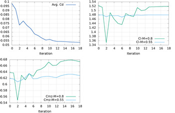
The optimisation histories are presented in Fig. 18. The two-point optimisation converged successfully after less than 20 design iterations and the lift and thickness constraints are met. The two-point case, compared to the single-point optimisation shows poorer performance at the nominal flight conditions. The average drag coefficient is reduced from 981 counts to 532 counts, 25 counts higher than the single-point case, while the averaged drag coefficient is reduced by 45.7%.

Figure 18.

Average drag, lift and pitch moment coefficients histories for the two-points wing optimisation.

The thickness distribution in the nominal conditions (M = 0.8) obtained in the two-point optimised wing is different than the single-point case. The optimisation algorithm allows less thickness reduction of nearly 20%, compared to the single-point optimised wing (see Fig. 19). The thickness reduction was the main driver for the shock elimination in the single-point. The multi-point optimisation resulted in a compromise between the two flight conditions, resulting in a shock-free solution. The resulted two-point optimised wing is more twisted than the single-point optimised wing, with a maximum negative outboard twist of ${5^\circ }$ at the wing tip. The main reason for that is the need to meet the lift constraint in the subsonic flow conditions.

Figure 19.

Twist (left) and thickness (right) distribution along the two-point optimised wing span compared to the single-point optimised design. The results are for the nominal flow conditions (M = 0.8).

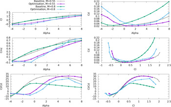
The two-point optimised configuration is used to compute a drag polar for both cases. Figure 20 shows the lift and drag coefficients vs. angle-of-attack and the drag polar for the two-point optimised wing, compared to the baseline wing configuration at Mach numbers 0.55 and 0.8. The drag polar shows that the drag reduction relative to the baseline curve improves at increased Cl, in the subsonic case (M = 0.55) but leads to significantly better drag performance at M = 0.8. The aerodynamic efficiency (Cl/Cd) is marginal for $\alpha = {3^\circ }$ and $Cl = 1.25$. Although, at positive angles of attack, there is a significant advantage to the optimised wing over the baseline configuration, in terms of manoeuvering capabilities and aerodynamic efficiency (flight distance).

Figure 20.

Polar graphs generated by the two-point optimised geometry and compared to the baseline wing configuration.

4.6 Single-point optimisation while starting from a random deformed geometry

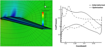
In order to examine the issue of multi-local minima, an optimisation starting from a deformed wing geometry is performed, similar to few impressive studies [Reference Chen, Lyu and Martines10, Reference Lee, Koo, Telidetzki, Buckley, Gagnon and Zingg27]. The baseline geometry is deformed by using Sculptor commercial software [28], by perturbing the wing surface in the chordwise and spanwise directions. In order to avoid any uncertainties relating to the grid convergence issues the same mesh topology is used (mesh level L1) for the deformed geometry. As expected, the performance of the initial design is poor, as is presented in Fig. 21 for the spanwise ${C_p}$ and sectional distribution.

Figure 21.

a) Pressure coefficient distribution over the initial deformed wing (left), and a comparison of the sectional Cp distribution at the middle wing span (right).

The initial deformed design is well reflected by the optimiser convergence behaviour, while the perturbation in the aerofoil thickness results in a bad initial design. The oscillating thickness distribution causes a chaotic pressure coefficient distribution, although the RANS solution converged well to the tolerance defined, within 40 design iterations. Despite the rather poor initial design, the gradients point in the right direction, and the wing is smoothed out and finally a shock-free geometry is obtained.

This problem is solved twice with different number of design variables. The first attempt includes 192 design variables on the wing, and within 30 design iterations the drag coefficient is reduced from 1,631 counts to 743 counts (54%), still higher than the single-point optimised wing (557 counts). Two possible reasons for this difference in the final design are as follows: first, the optimiser is not allowed to change the thickness of the 30% inboard wing, and as a result all the initial deformations could not be smoothed. Second, accumulated experience shows that the number of design variables, and mainly their distribution in the chordwise direction compared to the wing initial deformation, has a large impact on the optimisation process. For better performance the distance between two adjacent DV should be in the same order as the predicted mesh deformation, in a way that the deformed geometry could be visualised by the wing parametrisation. Therefore, increasing the distribution of control points along the chord and span directions will affect the design space, which means that the shape can be parametrised by the FFD.

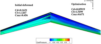
The second attempt includes 384 design variables (48 chordwise and 8 spanwise) and after 40 design iterations Cd is reduced to 591 counts, only 34 counts higher than the single-point optimised wing while starting from the baseline geometry. A comparison of the Cp distribution between the initial deformed configuration and the optimised wing is presented in Fig. 22. Despite the wild initial geometric conditions, a shock-free optimised wing is obtained. The increased number of design variables caused the optimiser to explore shapes with more curvature variation. This difference in the final optimised solutions may also be an indication of the multi-modality of the single-point-shape optimisation problem.

Figure 22.

A comparison (mirrored view) of the pressure coefficient distribution on the upper surface of the deformed wing (left) and the single-point optimised wing while starting from a deformed configuration (right). The results obtained with mesh level L1.

4.7 Optimising the wing with estimated trim penalty

The optimisation cases described in the previous chapters include the drag reduction of the wing only (connected to a symmetry plane). Practically we can ask how the optimised performance would be affected by a trimmed gliding wing configuration (which includes also body and stabilisers)? that is to say, what would be the drag reduction for a trimmed gliding configuration while the trimming is done by rotating the stabiliser. There are two approaches to answer this question. First, a complicated approach is to formulate an optimisation problem that includes the wing-body-stabiliser configuration, while the trimming is done by rotating the stabiliser as a solid body, as it is well established by Chen et al. [Reference Chen, Lyuy, Gaetan and Matines13]. The second and simpler approach is to use an aerodynamic derivatives model in order to formulate the drag coefficient as an objective which takes into account the trimming effect. The trimmed Cd is defined as:

\begin{equation} C{d_{trim}} = C{d_{trim\_orig}} + \Delta C{d_{wing\_new}} + \Delta C{d_{\delta p}} \end{equation}

Where $C{d_{trim\_orig}}$the total is drag defined in the aerodynamic model, $\Delta C{d_{win{g_{new}}}} = C{d_{win{g_{new}}}} - \;C{d_{win{g_{baseline}}}}$ represents the difference between the current (iterated) design and the baseline configuration. The stabiliser’s contribution to the trim process is defined as:

\begin{equation} \Delta C{d_{\delta p}} = C{d_{\delta {p^2}}}\Delta \left[ {\delta {p_{new}}^2 - \delta {p_{baseline}}^2} \right] \end{equation}

While the stabiliser’s rotation angle constraint for trimming is evaluated by moment balancing:

\begin{equation} \delta {p_{baseline}} = - \frac{{C{m_{wing\_baseline}}}}{{C{m_{\delta p}}}} \end{equation}

\begin{equation} \delta {p_{new}} = - \frac{{C{m_{wing\_new}}}}{{C{m_{\delta p}}}} \end{equation}

All the aerodynamic model coefficients for M = 0.8 are listed in Table 11

Table 11.

Aerodynamic model coefficients for trimmed flight in M = 0.8

Finally, the lift coefficient constraint ($C{l_{new}})$ is obtained by subtracting the stabiliser’s lift contribution due to the rotation from the baseline lift coefficient:

\begin{equation} C{l_{new}} = C{l_{baseline}} - C{l_{\delta p}} \cdot \delta {p_{new}} \end{equation}

Given this simplified model of the trim penalty generated by the moment required to trim the wing-body-stabiliser configuration, we can optimise the wing only (half configuration) without the body and stabiliser.

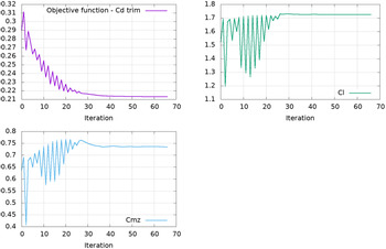
A single-point optimisation is performed with the same flight conditions, namely M = 0.8 (H = 7010m) with $C{d_{trim}}$ as the objective and $C{l_{new}}$ as the constraint (as well as thickness constraints). Convergence is reached within 8.8 hours using 4 processors (for mesh level L1), with 67 calls to the objective function and 55 calls to the sensitivity analysis function. The convergence history of the aerodynamic coefficients is shown in Fig. 23. The optimised wing has a 26.5% lower drag than the baseline configuration. The drag coefficient decreased by 769 counts, from Cd = 0.29 to Cd = 0.2131.

Figure 23.

Drag, lift and pitch moment coefficients histories for the wing optimisation with trim penalty.

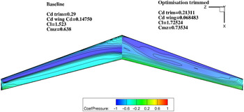
Figure 24 shows a comparison of the trimmed optimised and baseline wings, with the pressure coefficient distribution on the wing’s upper surface. It is clearly seen that the shape design variables make a significant contribution to minimise the drag. The initial geometry exhibits a front of very closely spaced pressure contour lines while the trimmed optimised wing shows a nearly shock-free solution.

Figure 24.

A comparison (mirrored view) of the pressure coefficient distribution on the upper surface of the baseline wing (left) and the single-point trimmed optimised wing (right). The results obtained with mesh level L1.

The thickness constraints are satisfied and the thickness of the inboard wing is increased by 5% compared to the initial design. The outboard wing thickness is reduced by nearly 25% the lower limit defined.

From the results presented in this section we can learn that for the single-point aerodynamic optimisation of the wing with no trim penalty in transonic flow, the lowest drag is achieved. Optimising the wing in two points (transonic and subsonic regimes) results in modest low drag predictions, mainly a result of the reduced wave drag. Optimising the wing with the trim penalty derived by an aerodynamic model, can also achieve a low drag values, and leads to a more practical design.