





1. Introduction
1.1. Literature review
An extensive discussion of the literature on the subject of blunted-cone capsules was presented in Part 1 (Hornung, Martinez Schramm & Hannemann Reference Hornung, Martinez Schramm and Hannemann2019). Here we restrict ourselves to a short summary of the results of Part 1. The two basic elements of a spherically blunted cone, the sphere and the sharp cone, were considered separately. Using a a large number of inviscid, perfect-gas computations, analytical relationships were found that fit in with hypersonic similarity theory. Analytical functions of two independent variables, the inverse normal-shock density ratio  $\varepsilon$ and
 $\eta$, a cone angle parameter that depends on the cone half-angle
 $\theta$ and
 $\varepsilon$, were found, in place of the unknown functions of the three independent variables (free stream Mach number
 $M_\infty$, specific heat ratio
 $\gamma$ and
 $\theta$) for the dimensionless shock wave stand-off distance
 $\varDelta /R$ (for precise definition see § 1.2), and the drag coefficient
 $C_D$. Here
 $R$ is the radius of the capsule, see figure 2. An analytical form was also found for
 $\varDelta /R$ in flow over geometries in the transition from the 90
 $^\circ$ cone to the sphere. The analysis was repeated for the case of the cone with a 10 % rounded shoulder that is relevant to the more realistic capsule shapes studied in Part 2. The relevance of the perfect-gas results of Part 1 to high-enthalpy non-equilibrium flows was foreshadowed. Inviscid computations of flows past a blunted cone configuration were used to explain the inflection point in the shock shape in the sphere-behaviour range.
1.2. Notation
Here  $x$ and
 $z$ are the streamwise and radial coordinates with origin at the stagnation point,
 $u$ is the
 $x$-component of velocity,
 $p$,
 $\rho$,
 $h$ and
 $T$ denote pressure, density, specific enthalpy and temperature, respectively . Here
 $M$ and
 $\gamma$ denote Mach number and specific heat ratio. The subscripts
 $\infty$ and 0 define free stream and reservoir values, respectively. Geometrical variables are defined in figure 2. The cone half-angle
 $\theta _d$ is the value of
 $\theta$ at shock detachment from a sharp cone. The shock stand-off distance
 $\varDelta$ is the distance between the point where the stagnation streamline crosses the shock and the stagnation point. The length in the Reynolds number
 $Re$ is 1 m.
1.3. Objectives
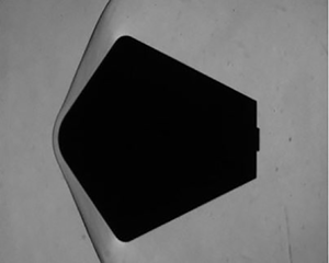
The emphasis of Part 2 is to extend the studies of Part 1 to blunted-cone capsules. In order to analyse the transition between sphere and cone behaviour and to compare the results with the analytical functions derived for  $\varDelta /R$ and
 $C_D$ for the sharp cone in Part 1, we perform a combined experimental and numerical study. The experiments are conducted in the High Enthalpy Shock Tunnel Göttingen (HEG) of the German Aerospace Centre using air as the test gas. The computational fluid dynamics (CFD) analysis is performed using the DLR TAU code. Since the sphere behaviour has been studied in detail in previous studies (see e.g. Stulov Reference Stulov1969; Wen & Hornung Reference Wen and Hornung1995), emphasis is placed here on the cone behaviour.
The experiments are performed with blunted-cone capsule models with ranges of  $\theta$ and
 $R_N$ and high-speed cinematography is applied to evaluate the development of
 $\varDelta /R$ and
 $C_D$. While Part 1 analysed perfect-gas flows, the shock layer flow generated at the selected HEG operating condition is in vibrational non-equilibrium. Accordingly, results will be compared with numerical predictions using different physico-chemical models to highlight their impact on the solutions. These computations also take viscous effects into account.
In a first step the shock layer flow is characterised by comparing the measured values of  $\varDelta /R$ and
 $C_D$ with numerical results obtained by applying different thermo-chemical relaxation models.
Second, computations are made using the free stream conditions of the selected HEG operating condition and the appropriate high temperature relaxation model on the configurations in Part 1, i.e. sharp cones with sharp shoulder (§ 4 in Part 1) and sharp cones with round shoulder (§ 5 in Part 1), both over a range of  $\theta$, as well as the transition from a 90
 $^\circ$ cone to a sphere (§ 5 in Part 1). These provide tests of the validity of the analytical functions of Part 1 and of the speculation that the functions derived for the cone behaviour also apply to flow fields including high temperature relaxation effects if the normal-shock density ratio is replaced by the density ratio based on the average density along the stagnation streamline.
The third step concentrates on the comparison and applicability of the analytical functions of Part 1 with the experimental and numerical results for blunted-cone configurations. For this purpose we aim to construct a model for the density profile along the stagnation streamline that permits an extension of the analytical function to vibrationally relaxing flows.
2. Experimental and numerical techniques
2.1. The HEG
The experiments are performed in the HEG of the German Aerospace Center, DLR. The HEG is a free-piston-driven reflected-shock wind-tunnel, capable of simulating a wide range of hypersonic flow conditions from the lower total specific enthalpy end up to representative re-entry conditions. Further information regarding the facility, which was commissioned for use in 1991, is provided, for example, in Hannemann (Reference Hannemann2003) and Hannemann & Martinez Schramm (Reference Hannemann and Martinez Schramm2007). Subsequent extensions of the HEG operating range included the establishment of a range of low total specific enthalpy conditions. Details are described, e.g. in Hannemann, Martinez Schramm & Karl (Reference Hannemann, Martinez Schramm and Karl2008), Hannemann et al. (Reference Hannemann, Martinez Schramm, Wagner, Karl and Hannemann2010) and Laurence (Reference Laurence2012).
For the present investigation, experiments were performed using HEG operating condition H3.3R3.7 (formerly referred to as condition XIII), which generates a representative free stream for an anticipated flight altitude of 28 km and a Mach number of  $M_\infty = 7.4$. Typical reservoir and free stream properties are provided in table 1. The reservoir pressure,
 $p_0$ was directly measured, while the reservoir enthalpy,
 $h_0$, was calculated using a standard routine by Krek & Jacobs (Reference Krek and Jacobs1993). The free stream conditions were determined by computing the nozzle expansion (see Hannemann et al. Reference Hannemann, Martinez Schramm, Wagner, Karl and Hannemann2010) with the DLR TAU code (see § 2.4) Though this computation accounted for chemical and vibrational non-equilibrium, the gas is fully recombined and vibration is in equilibrium at the nozzle exit. In figure 1, typical traces of the reservoir pressure, free stream static pressure and free stream Pitot pressure are plotted. The nominal test-time window of approximately 3 ms is also indicated in the figure. It is terminated by the arrival of expansion waves in the reservoir, resulting in steadily decreasing pressures thereafter. As discussed in Laurence et al. (Reference Laurence, Butler, Martinez Schramm and Hannemann2017) the unsteadiness in the reservoir pressure during the test period is typically of the order of 3.5 % standard deviation about the mean pressure. Estimated single-run uncertainties at this low-enthalpy condition in HEG are 5 % in
 $p_0$ and 4 % in
 $h_0$, with run-to-run variability being of the same order; corresponding uncertainties in the free stream properties are estimated as 5 % in
 $p_\infty$ and
 $\rho _\infty$, 3 % in
 $T_\infty$, 2 % in
 $u_\infty$, and 0.3 % in
 $M_\infty$.
Reservoir and free stream conditions for HEG operating condition H3.3R3.7.

Typical temporal development of the nozzle reservoir pressure (shifted in time to account for the delay between shock reflection at  $t = 0$ ms and the initiation of the flow in the test section), free stream static pressure and free stream Pitot pressure; HEG operating condition H3.3R3.7 (formerly referred to as condition XIII).

2.2. Wind tunnel model configurations
For a first set of models, the cone half-angle  $\theta$ ranged from 54
 $^\circ$ to 90
 $^\circ$ with nose radii of
 $R_N = 8$, 16 and 24 mm. All other parameters given in figure 2 remain fixed: the radius of the capsule
 $R = 40$ mm; the shoulder radius
 $R_S = 4$ mm; the base angle
 $\theta _B = 27^\circ$; and the base radius
 $R_B = 14.76$ mm. As a consequence, varying
 $\theta$ results in wind tunnel models with different axial lengths. A second set of models is used to quantify the influence of the shoulder radius. Starting from a 90
 $^\circ$ cone with
 $R_S/R = 0.1$, this parameter is increased in steps of 0.1 until a sphere (
 $R_S/R = 1.0$) is reached. The radius
 $R$, the base angle
 $\theta _B$ and the base radius
 $R_B$ are chosen according to the blunted cone models. The models are manufactured from high strength aluminium (brand name Weldural) and the typical mass is
 $300\,{\rm g} < m < 800$ g (see figures 3 and 4).
Schematic of spherically blunted cone capsules.

Blunted cone wind tunnel models: (a) varying  $\theta$, (
 $R_N = 8$ mm); (b)
 $\theta =62^\circ$,
 $R_N= 4$, 8, 16 and 24 mm from left to right.

Wind tunnel models used to study the influence of the shoulder radius (transition from a 90 $^\circ$ cone to a sphere).

2.3. Diagnostic techniques
The quantities of interest are  $\varDelta /R$ and
 $C_D$. Here, both quantities are determined based on high-speed schlieren cinematography of freely flying capsule models in the HEG test section. Details of the free flight technique applied in HEG are discussed in Laurence et al. (Reference Laurence, Butler, Martinez Schramm and Hannemann2017), who used this technique combined with optical-tracking for aerodynamic testing of a reduced-scale blunted-cone ExoMars entry capsule. Drag, lift and pitching-moment coefficients were determined and excellent agreement was obtained between the optical tracking technique and internally mounted accelerometer measurements. Preliminary results of test campaigns using the present model configurations and further details regarding the experimental technique are reported in Martinez Schramm, Hannemann & Hornung (Reference Martinez Schramm, Hannemann and Hornung2017, Reference Martinez Schramm, Hannemann and Hornung2019).
For the free-flight force measurement technique, the capsule models are integrated in the test section prior to a run by suspending them from the test section ceiling with two 150  $\mathrm {\mu }$m diameter Kevlar threads. These are glued into 0.5 mm diameter holes drilled in the model at the axial position of the model centre of mass and separated symmetrically by 60
 $^\circ$ along the circumference. All experiments were conducted at zero angle of attack. Special attention was paid to the accuracy of the model alignment. The misalignment of angle of attack and yaw angle were less than 0.03
 $^\circ$ relative to the centreline of the nozzle. The mounting of the capsule models in the HEG test section is shown in figure 5.
Schematic (a) and photograph (b) of the model suspension in the HEG test section.

The optical set-up used for the high-speed cinematography is shown in figure 6. The Z-type schlieren system includes the Cavitar Cavilux laser light source, the spherical mirrors (H1) positioned on either side of the test section, the secondary mirror (M) and the convex lens (L) which focuses the light beam on the chip of the high-speed Phantom V1210fast camera. At the focal point of lens (L), a vertical knife edge (R) may be placed to enhance the flow structure visualisation and to enable the determination of the shock-shape and the shock stand-off distance. The vertical centre plane of the model is imaged onto the focal plane (FP) of the camera.
Schematic of the high-speed cinematography optical set-up: H1, parabolic main mirrors; M, flat mirror; R, razor blade; L, convex lens; FP, focal plane.

The temporal evolution recorded during a typical run in HEG is summarised in figure 7 showing a blunted-cone model with  $\theta =69^\circ$. The red dotted line marks the initial position of the model leading edge. Frame 15 shows the model prior to the flow arrival. After flow arrival (frames 30 and 32) the threads separate from the model (frames 40, 45 and 47). The thread separation time can be determined from the recorded movies and is typically approximately 67
 $\mathrm {\mu }$s. Frames 75, 120 and 195 show the subsequent movement of the model.
Temporal evolution recorded during a typical HEG run applying the model free-flight technique. The time scale starts at shock reflection (SR) of the initial shock wave at the shock tube end wall and the red dotted line marks the initial position of the model leading edge.

In order to recover the models after the termination of the test section flow, a catching device is used as shown in figure 8. One of the design features of the catcher is that its influence on the flow is minimal. An indication of this may be seen in figure 8(b) showing a schlieren image of the flow over the catcher by itself. Two schlieren images depicting the free flight phase of the model after separation from the Kevlar threads and after the termination of the steady test time window is shown in figure 9.
Model catching device: photograph (a); schlieren visualisation of the flow past the device without capsule model during the test time window (b).

Schlieren images depicting the free flight phase of the model after separation from the Kevlar threads at approximately 4 ms after shock reflection (a) and after the termination of the test time window (3.5–6.5 ms) at approximately 19 ms (b).

The optical tracking algorithm matches the analytical model geometry specification to the image of the model recorded by the digital camera. The outputs of the algorithm are the position, angle of attack and scale of the model in each frame. Detailed discussion of the algorithm concept and its development is given by Laurence & Hornung (Reference Laurence and Hornung2009), Laurence & Karl (Reference Laurence and Karl2010), Laurence (Reference Laurence2012) and Laurence et al. (Reference Laurence, Butler, Martinez Schramm and Hannemann2017).
A short summary of the individual steps is given here. Firstly, the digital images are treated with an edge detection routine. Edge detection filters according to Sobel (Reference Sobel1970) or Canny (Reference Canny1986) are typically applied. Based on the measured pixel-intensity gradients and a predefined gradient threshold, a first set of pixels representing the model contour is determined. A parameterised representation, generally based on the position of the model centre of mass and vectors defined by the distance between the centre and the edge points and the corresponding polar angle are then used for the analytical contour and the points identified with the edge detection filter. The root mean square (r.m.s.) residual resulting from the comparison between the analytical and the detected edge points provides the indicator to judge the quality of the contour reconstructed from the digital images. The final model contour reconstruction (model horizontal and vertical position, angle of attack and scaling factor between the real geometry and the digital image) is determined by minimising the r.m.s. values using a Levenberg–Marquardt iterative solver (see figure 10).
Application of optical tracking algorithm: digital schlieren image (a); first set of pixels by evaluation of pixel-intensity gradient (b); final model contour reconstruction (c).

The convergence of this procedure is improved by a removal scheme for outliers, i.e. points which are located farther away from the detected contour than a user-defined fraction of the variance of all determined summed squared differences (Martinez Schramm et al. Reference Martinez Schramm, Hannemann and Hornung2017). In order to determine the optimal user-defined outlier threshold and to determine the accuracy of the contour reconstruction, 200 digital images of the stationary blunted-cone model are analysed. A standard deviation of 0.7  $\mathrm {\mu }$m for the location of the centre of mass (
 $\sqrt {x^2 + z^2}$) can be obtained with the optical set-up used (see Martinez Schramm et al. Reference Martinez Schramm, Hannemann and Hornung2019).
A Savitzky–Golay filter is employed to smooth the data. Its advantage over other smoothing techniques (e.g. moving averages) is that it does not cut off high frequencies. It therefore does not introduce major distortions and preserves features such as local peaks. The filter is used with a sixth-order polynomial and a 64-point basis. Differentiation of the displacement with respect to time yields the velocity and subsequently the acceleration of the model (see black lines in figure 10). Aerodynamic forces are then obtained by multiplying the acceleration with the known model mass. Due to the low unsteadiness in the reservoir pressure during the test time window of approximately 3.5 %, it is expected that the acceleration of the models is approximately constant during the test period. Consequently, the measured displacement should follow a quadratic function of the form
 \begin{equation} x(t)=c_1 t^2+c_2 t+c_3, \end{equation}
with the model acceleration  $a=2c_1$. Using the least squares method, a quadratic polynomial is fitted to the displacement. Evaluating the standard deviation of
 $c_1$ yields the uncertainty in the measured accelerations (see figure 11) which typically amounts to
 $\pm$0.35 % (Friedl, Martinez Schramm & Hannemann Reference Friedl, Martinez Schramm and Hannemann2015).
Evaluation of optical tracking data: Displacement (a), velocity (b), acceleration (c); the red lines represent the quadratic fit of the displacement and its first and second time derivative.

In a schlieren image with vertical orientation of the razor blade, the pixel intensity is related to the streamwise component of the density gradient. However, because the image results from a line-of-sight integration of the density gradient, the shock width in the image is broadened. In measuring the shock stand-off distance we therefore take the most upstream location of the change of pixel intensity to be the shock location. As an example, figure 12 shows the averaged streamwise normalised pixel intensity gradient,  $(\partial {I}/\partial {x})/(\partial {I}/\partial {x})_{max}$ along the stagnation streamline of a blunted cone with
 $\theta =69^\circ$ as a black line. The figure also shows the normalised streamwise second density derivative,
 $(\partial ^2{\rho }/\partial {x}^2)/(\partial ^2{\rho }/\partial {x}^2)_{\rm max}$ from a computation of the same flow as a red line. Both quantities are normalised with their relative maxima at the shock position.
Comparison of the normalised streamwise pixel intensity gradient to the computed streamwise second density derivative along the stagnation streamline for a blunted cone configuration with  $\theta =69^\circ$ and
 $R_N = 16$ mm (a). Enlarged view near the shock wave (b).

Compared with the computed second density derivative, the broader experimental shock profile can clearly be seen. The black dots illustrate the pixel positions. The distance between two pixels is significantly larger than the resolution used for the numerical computations; the grid points of the computation are shown as red dots. In figure 12(b), showing an enlarged view of the shock position, the resolution of the digital images (the distance between two pixels), and the precision (standard deviation of the image frame averaged position) of the intensity gradient measurements in the shock leading edge region are also indicated. In both the experimental and the numerical data, the shock location is determined as the point where the second density derivative or the pixel intensity gradient reaches 20 % of its relative maximum. Based on the resolution and the precision of the shock position measurement, the uncertainty of the shock stand-off distance  $\sigma _\varDelta =\pm 58\,\mathrm {\mu }$m is derived for the measurement shown in figure 12. For the grid-converged numerical solution, the uncertainty of the shock stand-off distance determination amounts to
 $\sigma _\varDelta =\pm 32\,\mathrm {\mu }$m.
2.4. The DLR TAU code
The numerical investigations conducted in the framework of the present study are performed with the hybrid structured/unstructured Navier–Stokes solver DLR TAU (Gerhold Reference Gerhold2005; Schwamborn, Gerhold & Heinrich Reference Schwamborn, Gerhold and Heinrich2006; Hannemann et al. Reference Hannemann, Martinez Schramm, Wagner, Karl and Hannemann2010; Karl Reference Karl2010; Kroll, Langer & Schwöppe Reference Kroll, Langer and Schwöppe2014). The TAU code is a second-order finite volume solver for the Euler and Navier–Stokes equations in the integral form including the use of eddy-viscosity (Reynolds-averaged Navier–Stokes), Reynolds-stress or detached- and large-eddy simulations for turbulence modelling. Here, steady, laminar flows of a calorically perfect gas, as well as chemical and vibrational equilibrium and non-equilibrium flows are considered.
The AUSDMV flux vector splitting scheme is used with MUSCL (monotonic upstream-centred scheme for conservation laws) gradient reconstruction to achieve second-order spatial accuracy. The equilibrium properties are calculated from partition functions or look-up tables. In the case of chemical non-equilibrium, the fluid is considered to be a reacting mixture of thermally perfect gases, with a transport equation solved for each individual species. The chemical source term is computed from the law of mass action by summation over all participating reactions. Air is modelled with a five species ( ${\rm N}_2$,
 ${\rm O}_2$, N, O, NO), 17 chemical reaction scheme. The forward reaction rate is computed using the modified Arrhenius law and rate coefficients taken from Gupta et al. (Reference Gupta, Yos, Thompson and Lee1990). The backward rate is obtained from the equilibrium constant, which is derived directly from the partition functions of the participating species. The thermodynamic properties (energy, entropy, specific heat) are calculated using the partition functions.
It should be pointed out that our interest centres on vibrational non-equilibrium as is appropriate for the conditions of the experiments (see table 1). Nevertheless, the chemical non-equilibrium effects, though small, need to be included.
Knowledge of the composition of the gas mixture and the thermodynamic state of the individual species allows the transport properties of the reacting gas mixture to be computed using suitable mixture rules from Wilke (Reference Wilke1950) for viscosity and from Herning & Zipperer (Reference Herning and Zipperer1936) for thermal conductivity. For the consideration of vibrational non-equilibrium, the relaxation rates of the vibrational energy for vibrational–vibrational and vibrational–translational coupling are computed according to Klomfass (Reference Klomfass1995). Two vibrational temperatures for molecular nitrogen and oxygen are used. A fully catalytic wall boundary condition, i.e. local chemical equilibrium at the wall defined by the wall temperature of 300 K is applied for the species partial densities. The species diffusion fluxes are modelled using Fick's law, with an averaged diffusion coefficient for all species. This is computed using the laminar mixture viscosity, and a constant Schmidt number of 0.7.
For the zero angle of attack flows of this study, only two-dimensional (2-D)-axisymmetric flow fields need to be computed. Typical hybrid grids (quadrilateral cells at the wall and triangular cells away from the wall) are shown in figure 13. Starting from an initial grid, it is refined to improve the accuracy of capturing the bow shock position. In order to obtain a converged solution, a threshold level of a combination of the computed temperature, pressure and Mach number gradients is used as adaptation criterion. Grid convergence can typically be obtained after six adaptation steps. The final, adapted grids contain approximately 12 500 cells. The grid resolution at the wall was selected such that converged wall heat flux values could be obtained. This quantity was monitored and used to check the time convergence of the solutions.
Typical hybrid grids (quadrilateral cells at the wall and triangular cells away from the wall) used for the 2-D-axisymmetric flow field computations: initial grid (a) and adapted grid (b). Axes show distances in millimetres.

3. Characterisation of the shock-layer flow
The models for the first set of experiments were blunted cones with  $R_N = 16$,
 $R_S=4$ mm and a range of values of
 $\theta$ (see figure 2). Schlieren images of flow over these, at the conditions of table 1, are shown together with corresponding computed results in figure 14. This comparison gives a nice characterisation of sphere behaviour and cone behaviour evident particularly in the evolution of the sonic line. Also shown in the left-hand-most schlieren image is the appearance of the inflection point in the shock wave that has been discussed in Part 1.
Top subpanels: experimental schlieren images of flow over models with  $R_N = 16$ mm and
 $55^\circ \le \theta \le 60^\circ$. Bottom subpanels: corresponding computational results showing the shock as the left boundary and the sonic line (red). Note the evolution of the sonic line showing sphere behaviour in the first image from the left-hand side, a subsonic island in the second, and cone behaviour in the third, fourth, fifth and sixth images.

Computations are performed with three models for the test gas air: (a) perfect gas with  $\gamma = 1.4$, i.e. a frozen flow; (b) a gas in vibrational equilibrium and chemical non-equilibrium; and (c) a gas in vibrational and chemical non-equilibrium. The computed results shown in figure 14 are for case (c).
The measured and computed values of  $\varDelta /R_N$, determined by the method illustrated in figure 12, are plotted against
 $\theta$ in figure 15. The influence of the different physico-chemical models is clearly visible. The measured values are best fitted by the assumption of a chemical and vibrational non-equilibrium flow. As more modes become excited, from frozen to equilibrium flow, the minimum in
 $\varDelta /R_N$ decreases and the termination of sphere behaviour occurs at higher
 $\theta$. It may be expected that this effect will be further increased at higher
 $h_0$ conditions where non-equilibrium dissociation plays a larger role.
Measured and computed values of  $\varDelta /R_N$ plotted against
 $\theta$, for a model with
 $R_N=24$ mm. The computed values show results obtained with different physico-chemical models: chemical non-equilibrium and vibrational equilibrium (ch-neq/t-eq); chemical and vibrational non-equilibrium (ch-neq/t-neq); and frozen flow (ch-fr/t-fr). Note how the ranges of sphere behaviour (constant
 $\varDelta /R_N$) terminate at different values of
 $\theta$ for the three physico-chemical models. The measured values include error bars.

The important result and conclusion from this analysis is that non-equilibrium vibrational relaxation is mandatory for the correct flow modelling at this condition. At the low- $h_0$ conditions of table 1 we can, therefore, study flow fields in which vibrational relaxation is a dominant effect, thus providing bench mark data for the validation of the corresponding models used in CFD codes.
Figure 16 shows corresponding results for the streamwise force component,  $F_x$. Both figures 15 and 16 show that the precision of these measurements is sufficiently high to resolve the effects of vibrational non-equilibrium. This is quite remarkable in the case of the force measurements since forces are very insensitive to relaxation effects. To our knowledge, the precision of the force-measurement technology developed at the HEG has not been equalled in high-enthalpy reflected shock tunnels. However, the computed values in these figures assume the free stream conditions to be precisely known. It is therefore through the computations that the free stream uncertainty enters the comparison. Computations made with the extremes of
 $\rho _\infty$ and
 $u_\infty$ corresponding to the free stream uncertainty were therefore made in order to obtain the resulting uncertainty in the computed forces. This uncertainty is superposed in figure 16 in the form of shading. Although the low scatter in the measured forces indicates very good shot-to-shot repeatability, the free stream uncertainty dominates the comparison. One is almost tempted to use the force measurements to nail down the free stream conditions more precisely than working from the uncertainty of the nozzle reservoir conditions.
Measured and computed values of the streamwise force component  $F_x$ plotted against
 $\theta$ for the models of figure 15. The notation for the physico-chemical models used in the computations is the same as in figure 15. The measured values again include error bars. The shaded region indicates the uncertainty in the computed force resulting from the free stream uncertainties.

Having established that considering both vibration and dissociation to be in non-equilibrium best fits the experimental data at the conditions of table 1, all computations presented in subsequent sections use this physico-chemical model.
4. Extension of the analytical forms of Part 1 to vibrationally relaxing flow
In Part 1, analytical expressions of the form
 \begin{equation} \frac{\varDelta}{R}=\frac{\varDelta}{R}(\varepsilon,\eta) \end{equation}
were found to apply over a wide parameter range for perfect-gas flows over a number of different geometries. For example, in the case of the sharp cone with sharp shoulder,
 \begin{equation} \frac{\varDelta}{R}=F(\varepsilon,\eta)=\sqrt{\varepsilon}(1+\varepsilon/2) [1.15(\eta-0.075)+0.06(\eta-0.075)^2]. \end{equation}
Here
 \begin{equation} \varepsilon=\frac{\rho_\infty}{\rho_s}, \end{equation}
where  $\rho _s$ is the density immediately downstream of the detached normal shock, and
 \begin{equation} \eta=\frac{\theta- \theta_d}{{\rm \pi}/2-\theta_d}, \end{equation}
in which  $\theta _d$ is the cone half-angle at shock detachment, for which Hayes & Probstein (Reference Hayes and Probstein1959) give the excellent approximation
 \begin{equation} \theta_d=2\arctan\sqrt{\frac{2}{\varepsilon}}-\frac{\rm \pi}{2}. \end{equation}
Part 1 also speculates that (4.1) applies for non-equilibrium flows as well, if  $\varepsilon$ is replaced by
 \begin{equation} \bar{\varepsilon}=\frac{\rho_\infty}{{\bar\rho}}, \end{equation}
where  $\bar {\rho }$ is the average density over distance along the stagnation streamline between the shock and the stagnation point. The extension is based on a control-volume argument used by Stulov (Reference Stulov1969) and Wen & Hornung (Reference Wen and Hornung1995) from which it follows that it applies to
 $\varDelta /R_{sh}$, where
 $R_{sh}$ is the radius of curvature of the shock on the stagnation streamline. For spheres and circular cylinders,
 $R_{sh}$ is approximately proportional to the geometrical length scale of the body so that the extension using
 $\bar {\varepsilon }$ applies also to
 $\varDelta$ normalised by the body scale. For some body shapes this proportionality is not true, so that care must be exercised in applying it to such cases.
For spheres and circular cylinders considerable success has been found by approximating the stagnation line density profile with simple forms. The exponential approach function suggested by Wen & Hornung (Reference Wen and Hornung1995) has been adapted to the case of vibrational relaxation by Houwing et al. (Reference Houwing, Nonaka, Mizuno and Takayama2000). Belouaggadia, Olivier & Brun (Reference Belouaggadia, Olivier and Brun2008) used the ideal dissociating gas model to construct a more precise predictive scheme for non-equilibrium dissociating flows.
In this section we construct a model for determining an approximate value of  $\bar \varepsilon$ from the free stream conditions, a model that is suitable for our case of vibrational relaxation of air. At the conditions of the experiment the contribution of dissociation to the average density is so small that it can be neglected.
4.1. Shock and equilibrium stagnation point parameters
In order to estimate the average density along the stagnation streamline it is first necessary to determine the immediate postshock density  $\rho _s$ and the density reached at the stagnation point in an inviscid equilibrium flow,
 $\rho _e$. Here
 $\rho _s$ and the immediate postshock temperature
 $T_s$ are given by
 \begin{equation} \frac{\rho_s}{\rho_\infty}=\frac{\gamma+1}{\gamma-1+2/M_\infty^2},\quad \frac{T_s}{T_\infty}=\frac{2\gamma M_\infty^2-(\gamma-1)}{\gamma+1}\frac{\rho_\infty}{\rho_s}, \end{equation}
where  $M_\infty$ is the free stream Mach number. Since we are dealing with a mixture of diatomic gases,
 $\gamma =1.4$ for the frozen shock jump.
In vibrational non-equilibrium flow the density rise from the shock to an inviscid equilibrium stagnation point has two causes. One is the vibrational excitation causing a temperature drop and the other is the deceleration of the flow from its speed at the shock to zero at the stagnation point. In the context of the chemical non-equilibrium flows considered by Wen & Hornung (Reference Wen and Hornung1995) and Belouaggadia et al. (Reference Belouaggadia, Olivier and Brun2008), the latter could be neglected. This is no longer admissible here. Thus,
 \begin{equation} \rho_e=\rho_s+\rho_{ev}+\rho_{ed}, \end{equation}
where  $\rho _e$ is the equilibrium stagnation point density in an inviscid flow,
 $\rho _{ev}$ is the density rise caused by vibrational relaxation and
 $\rho _{ed}$ is the density rise caused by deceleration. In an ideal-gas flow (at high
 $M_\infty$)
 \begin{equation} \frac{\rho_{ed}}{\rho_s}=\kappa(\gamma)=\frac{[(\gamma+1)/2]^{2/(\gamma-1)}}{\gamma^{1/(\gamma-1)}}-1. \end{equation}
We approximate this rise by choosing  $\gamma =4/3$, corresponding to vibration being half excited. We note that Houwing et al. (Reference Houwing, Nonaka, Mizuno and Takayama2000) neglected
 $\kappa$.
To determine  $\rho _{ev}$, observe that each fully excited degree of freedom increases
 $\rho /\rho _\infty$ by
 $2m(M_\infty )$ where
 $m(M_\infty )$ is approximately equal to the ratio of
 $\rho _s/\rho _\infty$ to its value with
 $M_\infty$ set to
 $\infty$ in (4.7a,b). Thus we may write
 \begin{equation} \frac{\rho_{ev}}{\rho_\infty}=2 m(M_\infty)\sum_{i=1}^2c_i\phi_i, \end{equation}
where the  $c_i$ are mass fractions, subscript 1 for oxygen, 2 for nitrogen and the degrees of vibrational excitation at the equilibrium stagnation point are given by
 \begin{equation} \phi_i=\frac{(\theta_{vi}/2T_e)^2}{\sinh^2(\theta_{vi}/2T_e)} \end{equation}
with the characteristic vibrational temperatures  $\theta _{vi}$. The subscripts of
 $\phi$ and
 $\theta _v$ have the same meaning and
 $T$ is the temperature. Equations (4.8) to (4.11) combine to provide a relation between
 $\rho _e$ and
 $T_e$.
A second relation between  $\rho _e$ and
 $T_e$ may be obtained by approximating the pressure increase caused by deceleration to be isentropic, so that
 \begin{equation} \frac{\rho_e}{\rho_s}=\frac{T_s}{T_e} (\kappa+1)^\gamma, \end{equation}
again with  $\gamma =4/3$. Thus we have two simultaneous equations in
 $\rho _e$ and
 $T_e$ which may be solved by iteration.
4.2. The rate of change of density at the shock
The assumptions made by Wen & Hornung (Reference Wen and Hornung1995) were adapted by Houwing et al. (Reference Houwing, Nonaka, Mizuno and Takayama2000) for vibrational relaxation and led to the rate at which vibrational excitation causes the density of a fluid element to change as it leaves the shock, namely
 \begin{equation} \left(\frac{{\rm d}\rho}{{\rm d} t}\right)_s={-}{\sum_{i=1}^2\left[c_i\frac{{\rm d} e_i}{{\rm d} t}\right]_s}/ \left(\frac{\partial h}{\partial \rho}\right)_s. \end{equation}
Here, the partial derivative of specific enthalpy  $h$ with respect to density considers
 $h$ to be
 $h(p,\rho,e_i)$ where the
 $e_i$ are the specific vibrational energies. In our mixture of two diatomic species, this partial derivative is given by
 \begin{equation} \left(\frac{\partial h}{\partial \rho}\right)_s={-}\frac{7}{2}\frac{p_s}{\rho_s^2}. \end{equation}
Remember that the subscript  $s$ denotes values at the immediate postshock condition.
The rate of change of  $e_i$ is given by
 \begin{equation} \frac{{\rm d} e_i}{{\rm d} t}=\frac{e_{ei}-e_i}{\tau_i}, \end{equation}
where the equilibrium specific vibrational energy  $e_{ei}$ is
 \begin{equation} e_{ei}=\frac{\mathcal{R}_i\theta_{vi}}{\exp(\theta_{vi}/T)-1}, \end{equation}
where  $\mathcal {R}_i$ is the specific gas constant and
 $\tau _i$ is the vibrational relaxation time for species
 $i$ in the mixture of the two species. The
 $\tau _i$ are functions of temperature, pressure and composition and are determined by the vibrational relaxation model described in § 2.4. These quantities all need to be evaluated at the immediate postshock conditions where
 $e_i=0$ if the free stream temperature is much smaller than
 $\theta _v$.
The rate at which vibrational excitation causes the density of a fluid element to change as it leaves the shock may be translated into a gradient of density at the shock by virtue of the flow speed at the shock,  $u_s=u_\infty \rho _{\infty }/\rho _s$:
 \begin{equation} G_s=\left(\frac{{\rm d}\rho}{{\rm d} s}\right)_s=\frac{1}{u_s} \frac{{\rm d}\rho}{{\rm d} t}=\frac{2}{7}\frac{\rho_s^3}{\rho_\infty u_\infty p_s} \sum_{i=1}^2\frac{c_i e_{ei}(T_s)}{\tau_i}, \end{equation}
where  $s=x+\varDelta$ is the distance along the stagnation line from the shock.
4.3. Model of the density profile along the stagnation line
Following the ideas of Wen & Hornung (Reference Wen and Hornung1995) and Houwing et al. (Reference Houwing, Nonaka, Mizuno and Takayama2000) we model the relaxation process with the exponential approach function. However, since the relevant parameters have to be evaluated for both species in any case, we model them with two separate exponential approach functions. In addition we include the deceleration density rise, which we model as being linear in  $\xi =s/\varDelta$. Thus the model takes the form
 \begin{equation} \zeta=\frac{\rho-\rho_s}{\rho_e-\rho_s}=\sum_{i=1}^2 \left[a_i\left(1-\exp({-b_i\xi})\right)\right]+\frac{\kappa\rho_s}{\rho_e-\rho_s}\xi. \end{equation}
Introduce relaxation rate parameters
 \begin{equation} \varOmega_i=\frac{c_i e_{ei}}{\tau_i}\frac{2R}{u_\infty^3}, \end{equation}
which measure the dimensionless rates at which energy goes into vibrational relaxation at the shock. Comparing (4.18) with (4.17), the parameters in (4.18) become
 \begin{equation} a_i=\frac{\rho_{evi}}{\rho_e-\rho_s}\quad {\rm and} \quad b_i=\frac{4}{7}\frac{\rho_s^3 u_\infty^2}{\rho_\infty p_s \rho_{evi}}\frac{\varOmega_i \varDelta}{R}. \end{equation}
Equation (4.18) may be integrated in closed form to obtain the average
 \begin{equation} \bar\zeta=\int_0^1 \zeta\,{\rm d}\xi=\sum_{i=1}^2\left[a_i+\frac{a_i}{b_i} \left({\rm e}^{{-}b_i}-1\right)\right]+\frac{\kappa\rho_s}{2(\rho_e-\rho_s)}. \end{equation}
From this we can determine  $\bar {\varepsilon }$:
 \begin{equation} \frac{1}{\bar\varepsilon}=\frac{\bar\rho}{\rho_\infty}= \frac{\rho_e-\rho_s}{\rho_\infty}\bar\zeta+\frac{\rho_s}{\rho_\infty}. \end{equation}
Equation (4.22) constitutes a relation between  $\varDelta /R$ and
 $\bar \varepsilon$. For several geometries, Part 1 gives analytical functions of the form of (4.1) for non-relaxing flow which, according to the suggestion at the end of Part 1, may be extended to relaxing flow by replacing
 $\varepsilon$ by
 $\bar \varepsilon$. Thus, for any particular one of these geometries, we have two independent relations between
 $\varDelta /R$ and
 $\bar \varepsilon$ which may be solved for both by iteration. In this case we have the luxury of being able to use the computed value of
 $\varDelta$ as the first guess for each geometry, which makes the convergence immediate.
4.4. Parameter values for the conditions of the experiment
In this section we present the numerical values of the parameters determined from the free stream conditions of the experiment and the procedure described above in tabular form. Table 2 gives some gas properties and parameter values at the immediate postshock condition. Table 3 gives the conditions at an inviscid-flow equilibrium stagnation point. It is interesting to point out that the iterative method of determining  $\rho _e$ described in § 4.1 yields
 $\rho _e=0.185$ kg m
 $^{-3}$ in good agreement with the computational value 0.187 kg m
 $^{-3}$.
Gas properties and parameter values at immediate post normal-shock conditions.

Parameter values at an inviscid-flow equilibrium stagnation point.

4.5. Test of the model
In order to test the model we choose two quite different geometries with very different values of  $\varDelta$, see figure 17. The computed density profile is plotted together with (4.18) for these two cases in both dimensional and dimensionless coordinates. In the dimensional coordinates the contribution from relaxation to the density rise which, according to the model, is the same for all cases in these coordinates, is also shown. This illustrates the need to take
 $\kappa$ into account.
Stagnation-line density profiles for two cases. Red colour, capsule shape with  $\theta =63^\circ$ and
 $R_N=16$ mm; blue colour, 90
 $^\circ$ cone with sharp shoulder; circles, computation; red and blue curves, (4.18). (a) Dimensional coordinates. The green curve is the contribution from relaxation, applicable to all cases in these coordinates. (b) Dimensionless coordinates.

It is clear from the comparison of the computed and model profiles that the discrepancy between  $\bar \zeta$ as computed and as modelled is smaller than 4 % in both cases. Since both the computations and the determination of the model parameters start from precisely the same free stream conditions, the discrepancy reflects the effect of the approximations made in constructing the model, and is remarkably small.
It is interesting to observe how this discrepancy in  $\bar \zeta$ propagates into a discrepancy in
 $\bar \varepsilon$. Denoting the discrepancies by
 $\delta$, use (4.22) to write
 \begin{equation} \frac{\delta\bar\varepsilon}{\bar\varepsilon}= \frac{(\rho_e-\rho_s)\delta\bar\zeta}{(\rho_e-\rho_s)\bar\zeta+\rho_s}= \frac{\delta\bar\zeta}{\bar\zeta}\frac{1}{1+\rho_s/[(\rho_e-\rho_s)\bar\zeta]}. \end{equation}
Since  $\bar \zeta$ is always smaller than 1, the fractional discrepancy in
 $\bar \varepsilon$ is smaller than that in
 $\bar \zeta$ by a factor of approximately 5 and is thus less than 1 %. Of course, as in the case of the force computations, the uncertainty of the free stream conditions affects both computed and modelled results.
5. Application of the model to the experimental and computed results
5.1. The sharp-nose sharp-shoulder cone
Figure 18 shows pseudoschlieren images of the computed flow fields, in which the grey-shading is proportional to the magnitude of the density gradient. The images also show the sonic line in red. Values of  $\varDelta /R$ extracted from these computations according to the procedure described in figure 12 are plotted against
 $\theta$ and against
 $\eta$ in figure 19. Also, for comparison, the plots show both
 $\varDelta /R=F(\varepsilon,\eta )$ (4.2) and
 $\varDelta /R=F(\bar {\varepsilon },\eta )$. The latter agrees with the computations to within less than 2 %.
Pseudoschlieren images in which the grey-shading is proportional to the magnitude of the density gradient, and sonic line (red) from computations of flow over sharp cones with sharp shoulder. Here  $\theta$ varies in steps of 2.5
 $^\circ$ from 62.5
 $^\circ$ to 90
 $^\circ$ in (a–l), respectively.

Comparison of computed values of  $\varDelta /R$ with both
 $\varDelta /R=F(\varepsilon,\eta )$ and
 $\varDelta /R=F(\bar {\varepsilon },\eta ):$ (a) plot versus
 $\theta$; (b) plot versus
 $\eta$.

From the same computation the drag coefficient
 \begin{equation} C_D=\frac{2D}{{\rm \pi} R^2 \rho_\infty u_\infty^2} \end{equation}
may also be extracted. Here  $D$ is the drag
 \begin{equation} D=2{\rm \pi}\int_0^R (p-p_\infty)z\,{\rm d} z, \end{equation}
where  $p$ is taken to be the forebody surface pressure, the base pressure being assumed to be equal to
 $p_\infty$.
Computed and measured values of  $C_D$ may then be compared with the analytical forms from Part 1,
 \begin{equation} C_D=G(\varepsilon,\eta)=(2.055-0.865\sqrt{\varepsilon})(0.92+0.08\eta), \end{equation}
and its extension to relaxing flow
 \begin{equation} C_D=G(\bar{\varepsilon}, \eta). \end{equation}
This comparison is shown in figure 20.
Comparison of computed values of  $C_D$ with both
 $C_D=G(\varepsilon,\eta )$ and
 $C_D=G(\bar {\varepsilon },\eta )$.

5.2. Transition from  $90^{\circ }$ cone to sphere

By successively increasing the shoulder radius  $R_S$ starting from a 90
 $^\circ$ cone with sharp shoulder, a set of bodies may be defined that ranges from the 90
 $^\circ$ cone (
 $R_S=0$) to a sphere (
 $R_S=R$). In Part 1, the analytical form
 \begin{equation} \frac{\varDelta}{R}=H(\varepsilon,R_S/R)=1.12\left(1-0.301\frac{R_s}{R}\right) \sqrt{\varepsilon\left(1-\frac{R_S}{R}+\varepsilon\right)} \end{equation}
was found to describe the dimensionless stand-off distance for this set of bodies quite accurately. Flows over the models shown in figure 4 were computed and the models were tested experimentally at the conditions of table 1. The results are compared with both (5.5) and with its extension to relaxing flow,
 \begin{equation} \frac{\varDelta}{R}=H(\bar{\varepsilon},R_S/R) \end{equation}
in figure 21. The agreement is again very good.
Comparison of computed and experimental values of  $\varDelta /R$ with both
 $\varDelta /R=H(\varepsilon,R_S/R)$ and
 $\varDelta /R=H(\bar {\varepsilon },R_S/R)$ for the set of bodies that describe the transition from a 90
 $^\circ$ cone to a sphere.

For this set of models we can also compare experimental and computational results for the drag coefficient, see figure 22. This figure also shows three points at which analytical forms from Part 1 are available: the case of the sharp-shoulder 90 $^\circ$ cone, the 90
 $^\circ$ cone with
 $R_S=0.1R$ and the sphere. These analytical forms, with
 $\varepsilon$ replaced by
 $\bar {\varepsilon }$, are included in figure 22.
Comparison of computed and experimental values of  $C_D$. Also shown are three points from the analytical forms of Part 1 in the form of the extension to relaxing flow. Transition from 90
 $^\circ$ cone to sphere.

5.3. Sharp cone with rounded shoulder
Another shape for which analytical forms for  $\varDelta /R$ and
 $C_D$ were obtained is the case of the sharp cone with
 $R_S=0.1R$ and experimental and numerical results were generated for these models also. The analytical forms are
 \begin{equation} \frac{\varDelta}{R}=K(\varepsilon,\eta)=1.049\sqrt{\varepsilon} (1+0.55\varepsilon)[(\eta-0.075)+0.032(\eta-0.075)^2] \end{equation}
and
 \begin{equation} C_D=L(\varepsilon,\eta)=(1.9-0.94\sqrt{\varepsilon})(0.95+0.05\eta). \end{equation}
Equation (5.7) and its extension  $K(\bar {\varepsilon },\eta )$ to relaxing flow are compared with the numerical and experimental results in figure 23. Similarly, (5.8) and its extension
 $L(\bar {\varepsilon },\eta )$ to relaxing flow are shown in figure 24. In both cases very good agreement is again observed.
Comparison of computed values of  $\varDelta /R$ with both
 $\varDelta /R=K(\varepsilon,\eta )$ and
 $\varDelta /R=K(\bar {\varepsilon },\eta )$: (a) plot versus
 $\theta$; (b) plot versus
 $\eta$. Sharp cone with rounded shoulder.

Comparison of computed values of  $C_D$ with
 $L(\varepsilon,\eta )$ and with
 $L(\bar {\varepsilon },\eta )$ for the sharp cone with rounded shoulder at
 $R_S=0.1R$.

5.4. The capsule shape: blunt cone with rounded shoulder
Finally, the actual capsule shape, a blunt cone with rounded shoulder at  $R_S=0.1R$ is examined. In Part 1, it was found that (5.7) could be applied to this shape as well, if a correction (last term in (5.9)) was applied:
 \begin{align} \frac{\varDelta}{R}=1.049\sqrt{\bar{\varepsilon}}(1+0.055\bar{\varepsilon}) [(\eta-0.075)+0.032(\eta-0.075)^2]+\frac{R_N}{R}\left(\frac{1}{\sin\theta}-1\right). \end{align}
Flows over a number of such shapes with different values of the nose radius  $R_N$ were measured and computed at the conditions of table 1. The results are compared with each other and with (5.9) in figure 25. The agreement between all three forms is again very good.
Comparison of computed and experimental values of  $\varDelta /R$ with (5.9) for three different values of
 $R_N$. Capsule shapes.

6. Conclusions
An experimental, computational and theoretical study was made of vibrationally relaxing flow of air over various geometries relevant to the blunted cone capsule. The experiments used freely flying models to perform high-precision force measurements and high-speed schlieren cinematography in the HEG. The computations were for viscous non-equilibrium air flow. A model for the stagnation-line density profile was constructed that is determined by the free stream conditions. The model was used to give the analytical forms, derived in Part 1 for non-relaxing flow, predictive quality for vibrationally relaxing flow as well. The geometries studied comprised sharp cones with sharp shoulder, sharp cones with rounded shoulder, 90 $^\circ$ cones with varying shoulder radius to provide the transition to a sphere, and blunted cone capsule shapes. In all cases both for the dimensionless stand-off distance and the drag coefficient, the agreement between the experiments, the computations and the extension of the analytical forms of Part 1 to relaxing flow was very good.
Acknowledgements
Very sadly, one of the coauthors of this work, K. Hannemann, passed away during its preparation. He was a major contributor and will be sorely missed for a long time. We thank one of the reviewers for urging us to add the work described in § 4.
Declaration of interests
The authors report no conflict of interest.



