1 Introduction
The mixing of two or more scalars is a process relevant to several engineering, environmental and chemical applications, such as multi-component droplet evaporation (Tonini & Cossali Reference Tonini and Cossali2015), transport of temperature and salinity in the ocean (Yang, Verzicco & Lohse Reference Yang, Verzicco and Lohse2016), and distribution and reaction of air pollutants in street canyons (Zhong, Cai & Bloss Reference Zhong, Cai and Bloss2016). Differential diffusion is a term characterising the separate evolution of initially perfectly correlated scalars in a turbulent or laminar flow caused only by different molecular diffusivities. This phenomenon has been intensively investigated for decades. The first observation of differential diffusion was reported by Bilger (Reference Bilger1977) in a CH4 diffusion flame. Experimental and numerical studies using reactive but also non-reactive flows followed. Measurements of turbulent non-reacting liquid and gas-phase flows were performed to quantify differential diffusion (e.g. Saylor & Sreenivasan (Reference Saylor and Sreenivasan1998), Dibble & Long (Reference Dibble and Long2005), Brownell & Su (Reference Brownell and Su2008)). The general finding was an increase in differential diffusion with decreasing Reynolds number and increasing Schmidt-number ratio. Lavertu, Mydlarski & Gaskin (Reference Lavertu, Mydlarski and Gaskin2008) experimentally studied the dependence of differential diffusion on the jet radial location for two substances having a Schmidt-number ratio of 2.5. The study supported the hypothesis that differential diffusion is dominant at the interface of the jet and ambient fluid, see also Kerstein (Reference Kerstein1990). In addition, many non-reacting direct numerical simulations (DNS) investigating differential diffusion in isotropic turbulence are reported in the literature (e.g. Nilsen & Kosály (Reference Nilsen and Kosály1997), Yeung, Sykes & Vedula (Reference Yeung, Sykes and Vedula2000), Ulitsky, Vaithianathan & Collins (Reference Ulitsky, Vaithianathan and Collins2002)). These studies contribute to the understanding of the connection between small and large scales, and confirmed the presence of differential diffusion effects at large scales. Moreover, a Schmidt-number-dependent propagation of the scalar incoherency from small to large scales was demonstrated by Yeung et al. (Reference Yeung, Sykes and Vedula2000). A review of differential diffusion in both experimental and numerical studies is given by Lavertu et al. (Reference Lavertu, Mydlarski and Gaskin2008). A very recent study by Maragkos et al. (Reference Maragkos, Rauwoens, Fauconnier and Merci2014) used large-eddy simulations (LES) of a non-reactive H2/CO2 jet to analyse differential diffusion at different jet heights. However, to our knowledge, differential diffusion has not yet been analysed in a DNS of a non-reactive turbulent jet flow continuing the studies of Lavertu et al. (Reference Lavertu, Mydlarski and Gaskin2008) and Maragkos et al. (Reference Maragkos, Rauwoens, Fauconnier and Merci2014).
Recent studies have discovered the importance of the turbulent/non-turbulent (T/NT) interface to flow dynamics; a review is given by da Silva et al. (Reference da Silva, Hunt, Eames and Westerweel2014). The T/NT interface separates flow fields into turbulent and non-turbulent regions in free shear flows through vorticity and a sharp vorticity increase across the interface (Watanabe et al. Reference Watanabe, Naito, Sakai, Nagata and Ito2015). Due to high local gradients near the interface, molecular diffusion is expected to be important, which was confirmed by Watanabe et al. (Reference Watanabe, Naito, Sakai, Nagata and Ito2015). They showed that the molecular diffusion term is important in the vicinity of the interface and that it significantly decreases towards the turbulent core region. This implies that differential diffusion is also important at the interface. Detecting the T/NT interface is based on several criteria, e.g. the vorticity and the scalar criterion. Gampert et al. (Reference Gampert, Boschung, Hennig, Gauding and Peters2014a ) performed a comparison of these criteria in a turbulent shear layer, transporting a single passive scalar. A reasonable choice of both threshold values enables the detection of almost the same interface position. However, the passive scalar criterion is expected to be valid only for unity-Schmidt-number scalars (Watanabe et al. Reference Watanabe, Naito, Sakai, Nagata and Ito2015), since only these reveal a significant correlation with the vorticity interface position. The impact of different Schmidt numbers and diffusion coefficients on interface detection has not yet been analysed in detail, and this is one scope of this study.
Differential diffusion is a complex phenomenon that is not entirely understood, but its effects on turbulent scalar mixing are important. This study contributes to understanding of differential diffusion by analysing a DNS of a temporally evolving turbulent plane jet of two passive scalars with different Schmidt numbers. DNS provides highly resolved three-dimensional data and enables the accurate detection of the T/NT interface. Thus, to quantify the effect of differential diffusion, a normalised differential diffusion parameter is analysed. A transport equation for the scalar differences is evaluated to study the origin of differential diffusion, particularly by looking at the source term. Further, the separation between the passive scalars is studied using conventional and conditional statistics with respect to the interface distance. The connection between large and small scales is analysed using scalar dissipation. Moreover, the physical mechanism responsible for the departure of the two scalars is analysed using the scalar gradient alignment, the ratio of the diffusive fluxes and by a transport equation for the scalar gradients.
2 Numerical approach
A direct numerical simulation of a temporally evolving turbulent plane jet flow was carried out. The set-up, albeit not directly comparable with a spatially evolving jet, yields similar flow features and thereby enables a highly resolved DNS at a reasonably large Reynolds number with a high quality of the statistics. The DNS solves the non-dimensional incompressible Navier–Stokes equations and transport equations for passive scalars using a highly accurate approach (Gampert et al.
Reference Gampert, Boschung, Hennig, Gauding and Peters2014a
). The convective term is formulated in skew-symmetric form to reduce aliasing errors. The spatial derivatives are treated by a sixth-order compact Padé scheme (Lele Reference Lele1992). Temporal integration is performed by a low-storage, stability-preserving fourth-order Runge–Kutta scheme. The Poisson equation is solved in the spectral space by adapting a Helmholtz equation, see Cook, Cabot & Miller (Reference Cook, Cabot and Miller2004). The computational domain has periodic boundary conditions in streamwise
 $Ox$
and spanwise
 $Oy$
directions, and free-slip boundary conditions are used in the crosswise
 $Oz$
direction. The flow is statistically homogeneous in
 $xOy$
planes. The non-dimensional size of the domain is
 $L_{x}=6\unicode[STIX]{x03C0}$
,
 $L_{y}=6\unicode[STIX]{x03C0}$
and
 $L_{z}=12.5$
to ensure statistical convergence and independence from the boundary condition. The computational domain is discretised by
 $2816\times 2816\times 1500$
grid points, slightly coarsened towards the crosswise boundaries. The interfacial layer is resolved well with 14 grid points at the investigated time
 $t_{2}$
, and the Kolmogorov length scale
 $\unicode[STIX]{x1D702}$
equals the grid width
 $\unicode[STIX]{x0394}x$
. Statistics depend on the crosswise direction
 $z$
and time
 $t$
. The transport equations are non-dimensionalised by the initial maximum velocity
 $U_{max,0}$
, the initial jet thickness
 $H_{0}$
, and the maximum value of the initial scalar profile
 $\unicode[STIX]{x1D719}_{max,0}$
. They read
 $$\begin{eqnarray}\displaystyle & \displaystyle \frac{\unicode[STIX]{x2202}u_{j}}{\unicode[STIX]{x2202}t}+u_{i}\frac{\unicode[STIX]{x2202}u_{j}}{\unicode[STIX]{x2202}x_{i}}=-\frac{\unicode[STIX]{x2202}p}{\unicode[STIX]{x2202}x_{j}}+\frac{1}{\mathit{Re}_{0}}\frac{\unicode[STIX]{x2202}^{2}u_{j}}{\unicode[STIX]{x2202}x_{i}\unicode[STIX]{x2202}x_{i}},\quad \frac{\unicode[STIX]{x2202}u_{i}}{\unicode[STIX]{x2202}x_{i}}=0 & \displaystyle\end{eqnarray}$$
 $$\begin{eqnarray}\displaystyle & \displaystyle \frac{\unicode[STIX]{x2202}\unicode[STIX]{x1D719}_{\unicode[STIX]{x1D6FC}}}{\unicode[STIX]{x2202}t}+u_{i}\frac{\unicode[STIX]{x2202}\unicode[STIX]{x1D719}_{\unicode[STIX]{x1D6FC}}}{\unicode[STIX]{x2202}x_{i}}=\frac{1}{\mathit{Pe}_{0,\unicode[STIX]{x1D6FC}}}\frac{\unicode[STIX]{x2202}^{2}\unicode[STIX]{x1D719}_{\unicode[STIX]{x1D6FC}}}{\unicode[STIX]{x2202}x_{i}\unicode[STIX]{x2202}x_{i}},\quad \unicode[STIX]{x1D6FC}=1,2, & \displaystyle\end{eqnarray}$$
where
 $\unicode[STIX]{x1D6FC}$
does not indicate index summation. The Péclet number is defined as
 $\mathit{Pe}_{0,\unicode[STIX]{x1D6FC}}=\mathit{Sc}_{\unicode[STIX]{x1D6FC}}\mathit{Re}_{0}$
,
 $\mathit{Re}_{0}$
denotes the initial jet Reynolds number equal to 8000, and the Schmidt number
 $\mathit{Sc}_{\unicode[STIX]{x1D6FC}}$
is the ratio of kinematic viscosity
 $\unicode[STIX]{x1D708}$
and molecular diffusivity
 $D_{\unicode[STIX]{x1D6FC}}$
set to 1 for
 $\unicode[STIX]{x1D719}_{1}$
and to 0.25 for
 $\unicode[STIX]{x1D719}_{2}$
. The jet width
 $H$
is defined as the distance between the points at which the mean streamwise velocity decreases to 50 % of its centreline value. Subsequently, all given quantities are normalised in the same way. The initial velocity profile is composed of two mirrored hyperbolic-tangent mean profiles. Delta-correlated velocity fluctuations with an intensity of 5 % are superimposed onto the mean profile. This approach enables transition to turbulence without prescribing a length scale. The two mean scalar profiles are initialised corresponding to the mean velocity profile, but are non-perturbed and thus perfectly correlated.
3 Results and discussion
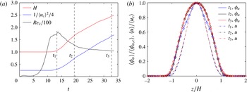
The jet transition to fully developed turbulence is illustrated in figure 1(a) using the jet width
 $H$
, the centreline mean streamwise velocity excess
 $1/\langle u_{c}\rangle ^{2}$
, and the Taylor micro-scale based Reynolds number
 $\mathit{Re}_{\unicode[STIX]{x1D706}}=\sqrt{15/(\langle \unicode[STIX]{x1D700}_{c}\rangle \unicode[STIX]{x1D708})}\langle u_{c}^{\prime 2}\rangle$
at the jet centre (index
 $c$
), where
 $\langle \unicode[STIX]{x1D700}_{c}\rangle$
is the mean centreline dissipation. After an initial transition, the first two quantities show a linear increase with time (Stanley, Sarkar & Mellado Reference Stanley, Sarkar and Mellado2002). Figure 1(a) also indicates the jet times that are used in the subsequent analyses. The self-similar decay is further illustrated in figure 1(b) by the normalised streamwise mean velocity profiles
 $u$
and the normalised mean scalar profiles for
 $\unicode[STIX]{x1D719}_{\unicode[STIX]{x1D6FC}}$
.
Temporal evolution of the jet thickness
 $H$
, the mean velocity excess
 $1/\langle u_{c}\rangle ^{2}$
and the Taylor micro-scale based Reynolds number
 $\mathit{Re}_{\unicode[STIX]{x1D706}}$
at the jet centre (a) and normalised mean scalar profiles (solid line:
 $\unicode[STIX]{x1D719}_{1}$
, solid line with symbol:
 $\unicode[STIX]{x1D719}_{2}$
) and streamwise velocity profiles at different times (b).

The first jet time considered is still in the transition regime, where the jet is not yet fully turbulent; thus, the scalar mean profiles have not reached the self-similar state. The jet times thereafter are within the fully turbulent self-similar regime and the normalised mean profiles collapse. In the following analysis, the jet time
 $t_{2}$
is used as the reference time and
 $t_{3}$
is used for parameter studies.
3.1 Detecting the T/NT interface
Several criteria can be used to detect the T/NT interface; see da Silva et al. (Reference da Silva, Hunt, Eames and Westerweel2014) for an overview. Gampert et al. (Reference Gampert, Boschung, Hennig, Gauding and Peters2014a ) showed that the scalar criterion and the vorticity criterion result in almost the same T/NT interfaces. Differences in the detected interface position for scalars with different Schmidt numbers are studied in the following section.
Detection of the interface position
 $z_{I}$
is based on a prescribed threshold of the vorticity or scalar. The threshold value of the scalar defining the scalar interface position can be found using a probability density function (p.d.f.) of the scalar at a crosswise position where the shape of the p.d.f. is bimodal. The scalar threshold value then equals the value where the minimum of this p.d.f. is found, see Prasad & Sreenivasan (Reference Prasad and Sreenivasan1989). In general, different threshold values are found for different scalar diffusivities and mixing states, e.g. for
 $t_{2}$
the values are 0.050 for
 $\unicode[STIX]{x1D719}_{1}$
and 0.045 for
 $\unicode[STIX]{x1D719}_{2}$
. With these threshold values, the interface position of
 $\unicode[STIX]{x1D719}_{1}$
(denoted as
 $z_{I,\unicode[STIX]{x1D719}_{1}}$
) and of
 $\unicode[STIX]{x1D719}_{2}$
(denoted as
 $z_{I,\unicode[STIX]{x1D719}_{2}}$
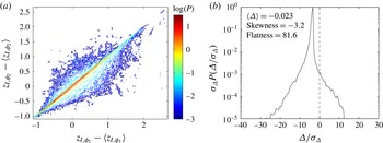
) are compared. The joint p.d.f.
 $P(z_{I,\unicode[STIX]{x1D719}_{1}}-\langle z_{I,\unicode[STIX]{x1D719}_{1}}\rangle ,z_{I,\unicode[STIX]{x1D719}_{2}}-\langle z_{I,\unicode[STIX]{x1D719}_{2}}\rangle )$
of the offset from the mean interface position
 $\langle z_{I,\unicode[STIX]{x1D719}_{\unicode[STIX]{x1D6FC}}}\rangle$
is shown in figure 2(a). The interface positions of both scalars are strongly correlated. However, there are also large differences between the two interface positions, albeit at low probability. Figure 2(b) shows the normalised marginal p.d.f.
 $\unicode[STIX]{x1D70E}_{\unicode[STIX]{x1D6E5}}P(\unicode[STIX]{x1D6E5}/\unicode[STIX]{x1D70E}_{\unicode[STIX]{x1D6E5}})$
of the difference
 $\unicode[STIX]{x1D6E5}=z_{I,\unicode[STIX]{x1D719}_{1}}-z_{I,\unicode[STIX]{x1D719}_{2}}$
, with
 $\unicode[STIX]{x1D70E}_{\unicode[STIX]{x1D6E5}}$
being the root mean square (r.m.s.) of
 $\unicode[STIX]{x1D6E5}$
. The p.d.f. is not centred, and a distinct peak at
 $\unicode[STIX]{x1D6E5}/\unicode[STIX]{x1D70E}_{\unicode[STIX]{x1D6E5}}=-3.4$
indicates that the two interfaces are correlated but slightly shifted. Moreover, the negative skewness and a relatively high flatness indicate the presence of large negative differences between the two interfaces.
Logarithmically scaled joint p.d.f. of the offset from the mean interface position
 $P(z_{I,\unicode[STIX]{x1D719}_{1}}-\langle z_{I,\unicode[STIX]{x1D719}_{1}}\rangle ,z_{I,\unicode[STIX]{x1D719}_{2}}-\langle z_{I,\unicode[STIX]{x1D719}_{2}}\rangle )$
(a) and normalised marginal p.d.f. of the difference between the interface positions
 $\unicode[STIX]{x1D70E}_{\unicode[STIX]{x1D6E5}}P(\unicode[STIX]{x1D6E5}/\unicode[STIX]{x1D70E}_{\unicode[STIX]{x1D6E5}})$
(b) detected with the scalar criterion of both scalars.

To analyse differential diffusion, a criterion for the interface detection is required that does not rely on the scalar field. Thus, the vorticity criterion was used to detect the interface position in the subsequent analyses. Following the approach of Bisset, Hunt & Rogers (Reference Bisset, Hunt and Rogers2002), parameter studies revealed that the threshold value of
 $\sqrt{6}$
for the non-dimensional vorticity, which comes from the non-dimensionalisation of (2.1) using
 $H_{0}$
and
 $U_{max,0}$
, is appropriate.
3.2 Differential diffusion
For quantification, the differential diffusion parameter
 $Z$
according to Lavertu et al. (Reference Lavertu, Mydlarski and Gaskin2008)
 $$\begin{eqnarray}Z=\frac{\unicode[STIX]{x1D719}_{1}}{\left<\unicode[STIX]{x1D719}_{1}\right>}-\frac{\unicode[STIX]{x1D719}_{2}}{\left<\unicode[STIX]{x1D719}_{2}\right>}\end{eqnarray}$$
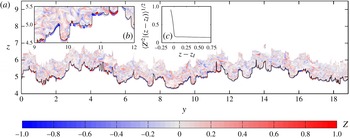
is evaluated. An instantaneous distribution of
 $Z$
in the
 $yOz$
plane is shown in figure 3(a). Note that only the lower interface is displayed and
 $Z$
is shown in a predefined band around the interface. Within the core region,
 $Z$
attains small finite values fluctuating around zero. Very large positive or negative values of
 $Z$
are obtained in the vicinity of the interface. Following the approach of Lavertu et al. (Reference Lavertu, Mydlarski and Gaskin2008), only the r.m.s. of
 $Z$
is analysed. This value conditioned on the distance from the interface
 $z-z_{I}$
is shown in figure 3(c), since
 $Z$
itself is a centred variable. It clearly indicates the dominance of differential diffusion at the interface. In the turbulent jet core, differential diffusion occurs locally but is an order of magnitude smaller compared to the magnitude at the interface.
Distribution of the differential diffusion parameter
 $Z$
in a
 $yOz$
plane in a predefined band around the lower T/NT interface (black line), detected with the vorticity criterion (a), zoom of the same distribution (b) and the distribution of its r.m.s. conditioned on the distance from the T/NT interface
 $z-z_{I}$
along the crosswise coordinate (c).

To quantify the absolute departure between the two scalars, the difference
 $\unicode[STIX]{x0394}\unicode[STIX]{x1D719}=\unicode[STIX]{x1D719}_{1}-\unicode[STIX]{x1D719}_{2}$
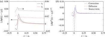
is introduced. The mean and r.m.s. of
 $\unicode[STIX]{x0394}\unicode[STIX]{x1D719}$
are presented in figure 4(a). The mean of the difference
 $\unicode[STIX]{x0394}\unicode[STIX]{x1D719}$
attains a negative mean value near the interface towards the irrotational side. Moving further towards the turbulent jet core results in a significant increase in the mean of
 $\unicode[STIX]{x0394}\unicode[STIX]{x1D719}$
before it approaches zero in the core region, which corresponds to the differences found in the mean scalar profiles, see figure 5(a). This does not imply that differential diffusion vanishes in the core region, as indicated by the non-zero r.m.s. of
 $\unicode[STIX]{x0394}\unicode[STIX]{x1D719}$
seen in figure 4(a).
The mean (solid line) and r.m.s. (dashed line) of the difference
 $\unicode[STIX]{x0394}\unicode[STIX]{x1D719}$
for two different jet times (a) and the terms of (3.2) conditioned on the distance from the T/NT interface along the crosswise coordinate at
 $t_{2}$
(b).

A transport equation for
 $\unicode[STIX]{x0394}\unicode[STIX]{x1D719}$
is given in (3.2) as similarly used by Bilger & Dibble (Reference Bilger and Dibble1982) to analyse the physical mechanism behind the observed differential diffusion
 $$\begin{eqnarray}\underbrace{\frac{\unicode[STIX]{x2202}\unicode[STIX]{x0394}\unicode[STIX]{x1D719}}{\unicode[STIX]{x2202}t}}_{\text{local changes}}+\underbrace{u_{i}\frac{\unicode[STIX]{x2202}\unicode[STIX]{x0394}\unicode[STIX]{x1D719}}{\unicode[STIX]{x2202}x_{i}}}_{\text{convection}}=\underbrace{\frac{1}{\mathit{Pe}_{0,1}}\frac{\unicode[STIX]{x2202}^{2}\unicode[STIX]{x0394}\unicode[STIX]{x1D719}}{\unicode[STIX]{x2202}x_{i}\unicode[STIX]{x2202}x_{i}}}_{\text{diffusion}}+\underbrace{\left(\frac{1}{\mathit{Pe}_{0,1}}-\frac{1}{\mathit{Pe}_{0,2}}\right)\frac{\unicode[STIX]{x2202}^{2}\unicode[STIX]{x1D719}_{2}}{\unicode[STIX]{x2202}x_{i}\unicode[STIX]{x2202}x_{i}}}_{\text{source term}}\,.\end{eqnarray}$$
Equation (3.2) contains the balance between the local changes, convection, diffusion and the source term. Note that the source term disappears when
 $Sc_{1}$
equals
 $Sc_{2}$
. To quantify the behaviour of the transport equation, the convection, diffusion and source terms are conditionally averaged and shown in figure 4(b). All terms of the transport equation for
 $\unicode[STIX]{x0394}\unicode[STIX]{x1D719}$
are large in the vicinity of the interface and tend to zero in the irrotational outer flow and the turbulent jet core. This is consistent with the distribution of
 $\unicode[STIX]{x0394}\unicode[STIX]{x1D719}$
shown in figure 4(a). Further, the convective term clearly dominates the balance equation. In contrast, the diffusion and the source terms are significantly smaller, but of the same order of magnitude. Since convection and diffusion only participate in distributing
 $\unicode[STIX]{x0394}\unicode[STIX]{x1D719}$
, the only term that generates differences in the two scalars is the source term, which only exists near the interface. Thus, differential diffusion clearly arises at the interface.
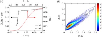
Since differential diffusion manifests itself as a deviation between the turbulent scalar fields, statistics of the two scalars and their differences are studied. Figure 5(a) shows the mean profiles of the two scalars, conditioned on the distance from the interface
 $z-z_{I}$
and conventionally averaged over the distance from the jet centre
 $z-z_{C}$
. High mean gradients of both scalars are visible in the conditioned statistics, whereas the standard averaging procedure results in flatter profiles. Differences between the two mean scalar profiles can only be seen in conditional statistics, while conventional averaging leads to almost congruent profiles. The reason is that conventional averaging mixes effects that are attributed to either the non-turbulent or the turbulent fluid regime. These findings are in line with those of Bisset et al. (Reference Bisset, Hunt and Rogers2002), who compared conventional and conditional statistics of the velocity field. Motivated by the differences in the conditional mean profiles, the joint statistics of both scalars at the interface are studied. The joint p.d.f.
 $P(\unicode[STIX]{x1D719}_{1},\unicode[STIX]{x1D719}_{2};z_{I})$
at the interface, shown in figure 5(b), illustrates the de-correlation of the scalars, induced by different diffusivities. Although
 $P(\unicode[STIX]{x1D719}_{1},\unicode[STIX]{x1D719}_{2};z_{I})$
reveals a distinct maximum, excursions indicating large differences occurring at low probability are present, and significant fluctuations arise around the nonlinear conditional mean
 $\langle \unicode[STIX]{x1D719}_{2}|\unicode[STIX]{x1D719}_{1};z_{I}\rangle$
.
Passive scalar mean profiles along the crosswise coordinate conditioned on the distance from the T/NT interface
 $z-z_{I}$
(black lines) and conventionally averaged as a function of the crosswise distance from the jet centre
 $z-z_{C}$
(red lines) (a). Joint p.d.f.
 $P(\unicode[STIX]{x1D719}_{1},\unicode[STIX]{x1D719}_{2};z_{I})$
of the passive scalars and the conditional mean
 $\langle \unicode[STIX]{x1D719}_{2}|\unicode[STIX]{x1D719}_{1};z_{I}\rangle$
(black line) (b).

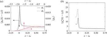
Mean scalar dissipation along the crosswise coordinate conditioned on the distance from the T/NT interface (black lines) and conventionally averaged (red lines) (a) and non-dimensional scalar dissipation conditioned on the distance from the interface (b).

Differential diffusion is molecular in origin and, according to Kolmogorov’s hypothesis, such effects should not be present at sufficiently high Reynolds numbers at large scales. However, Yeung (Reference Yeung1996) confirmed the presence of differential diffusion at both small and large scales, e.g. in the scalar dissipation and in the scalar variances. Thus, at first, statistics of the scalar dissipation are studied, defined as
 $$\begin{eqnarray}\unicode[STIX]{x1D712}_{\unicode[STIX]{x1D6FC}}=2D_{\unicode[STIX]{x1D6FC}}\frac{\unicode[STIX]{x2202}\unicode[STIX]{x1D719}_{\unicode[STIX]{x1D6FC}}}{\unicode[STIX]{x2202}x_{i}}\frac{\unicode[STIX]{x2202}\unicode[STIX]{x1D719}_{\unicode[STIX]{x1D6FC}}}{\unicode[STIX]{x2202}x_{i}}\,.\end{eqnarray}$$
Figure 6(a) shows the comparison between the conventionally and conditionally averaged scalar dissipation for both scalars. At the interface, the conditional mean scalar dissipation exhibits large values that stem from large local gradients. Differences in scalar dissipation are visible at the interface and also in the turbulent jet core for both averaging procedures. Next, to establish a connection between large and small scales and to analyse the effect of molecular diffusivity, a non-dimensional scalar dissipation is introduced
 $$\begin{eqnarray}\langle \unicode[STIX]{x1D712}_{\unicode[STIX]{x1D6FC}}^{\ast }|(z-z_{I})\rangle =\frac{\langle \unicode[STIX]{x1D712}_{\unicode[STIX]{x1D6FC}}|(z-z_{I})\rangle \unicode[STIX]{x1D70F}_{Z_{I}}}{\langle \unicode[STIX]{x1D719}_{\unicode[STIX]{x1D6FC}}^{\prime 2}|(z-z_{I})\rangle },\end{eqnarray}$$
as proposed by Obukhov (Reference Obukhov1949) and Corrsin (Reference Corrsin1951), where
 $\unicode[STIX]{x1D70F}_{Z_{I}}$
denotes the conditional mean integral time scale, defined as
 $\unicode[STIX]{x1D70F}_{Z_{I}}=\langle k|(z-z_{I})\rangle /\langle \unicode[STIX]{x1D700}|(z-z_{I})\rangle$
, where
 $k$
is the turbulent kinetic energy. The non-dimensional dissipation is used to discuss the impact of molecular diffusivity in the context of the dissipation anomaly first developed by Taylor (Reference Taylor1938) for the turbulent velocity. It postulates that the mean energy dissipation
 $\langle \unicode[STIX]{x1D700}\rangle$
becomes independent of viscosity provided that the Reynolds number is large enough. Similarly for passive scalars,
 $\langle \unicode[STIX]{x1D712}_{\unicode[STIX]{x1D6FC}}^{\ast }\rangle$
should approach a constant in the limit of large Péclet numbers. Figure 6(b) shows
 $\langle \unicode[STIX]{x1D712}_{\unicode[STIX]{x1D6FC}}^{\ast }\rangle$
conditioned on the interface coordinate for both scalars. The curves of both scalars collapse in the jet core region and approach a value of 2.5, which is in good agreement with the findings reported by Donzis, Sreenivasan & Yeung (Reference Donzis, Sreenivasan and Yeung2005) for a variety of different turbulent flows. This confirms Taylor’s postulate that non-dimensional scalar dissipation is independent of the molecular diffusivity. In contrast, towards the T/NT interface, both curves increase and depart significantly from each other, where the low-Schmidt-number scalar attains twice the peak value of the unity-Schmidt-number scalar. Departure in the vicinity of the T/NT interface indicates that normalised dissipation cannot be expressed solely by the large-scale quantities
 $\langle \unicode[STIX]{x1D719}^{\prime 2}\rangle$
and
 $\unicode[STIX]{x1D70F}_{Z_{I}}$
, but is also dependent on molecular diffusivity. This finding confirms the observations of Watanabe et al. (Reference Watanabe, Naito, Sakai, Nagata and Ito2015) that molecular diffusion is not negligible near the interface. In da Silva et al. (Reference da Silva, Hunt, Eames and Westerweel2014) it was reported that the edge of the turbulent jet flow consists of interfacial layers, in which turbulence does not reach a universal state. This changes the balance between large and small scales. These findings are also relevant for LES. An LES study concerning the T/NT interface was performed by Gampert et al. (Reference Gampert, Kleinheinz, Peters and Pitsch2014b
). It was shown that mean statistics of the T/NT interface are in reasonable agreement with experiments provided that the LES resolution is high enough. However when considering differential diffusion, sub-filter effects at the T/NT interface need to be modelled. Furthermore, accurately accounting for differential diffusion is crucial for turbulence–chemistry interaction models used in simulations of reactive flows.
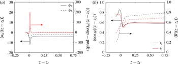
Strain acting in scalar gradient direction (black lines) and balance of production and dissipation term of (3.5) (red lines) (a) and cosine of the angle between the scalar gradients (solid line) and ratio of the absolute diffusive fluxes of the two passive scalars (dashed line) at two different jet times (b) conditioned on the distance from the T/NT interface along the crosswise coordinate.

The generation of local scalar gradients is analysed with a transport equation for the square of the scalar gradients
 $g_{\unicode[STIX]{x1D6FC}}^{2}=\unicode[STIX]{x1D712}_{\unicode[STIX]{x1D6FC}}/2D_{\unicode[STIX]{x1D6FC}}$
following Brethouwer, Hunt & Nieuwstadt (Reference Brethouwer, Hunt and Nieuwstadt2003)
 $$\begin{eqnarray}\frac{\unicode[STIX]{x2202}g_{\unicode[STIX]{x1D6FC}}^{2}}{\unicode[STIX]{x2202}t}+u_{i}\frac{\unicode[STIX]{x2202}g_{\unicode[STIX]{x1D6FC}}^{2}}{\unicode[STIX]{x2202}x_{i}}=\underbrace{-2g_{\unicode[STIX]{x1D6FC},j}s_{ij}g_{\unicode[STIX]{x1D6FC},i}}_{\text{production}}-\underbrace{\frac{2}{Pe_{0,\unicode[STIX]{x1D6FC}}}\frac{\unicode[STIX]{x2202}g_{\unicode[STIX]{x1D6FC},j}}{\unicode[STIX]{x2202}x_{i}}\frac{\unicode[STIX]{x2202}g_{\unicode[STIX]{x1D6FC},j}}{\unicode[STIX]{x2202}x_{i}}}_{\text{dissipation}}+\frac{1}{Pe_{0,\unicode[STIX]{x1D6FC}}}\frac{\unicode[STIX]{x2202}^{2}g_{\unicode[STIX]{x1D6FC}}^{2}}{\unicode[STIX]{x2202}x_{i}\unicode[STIX]{x2202}x_{i}}.\end{eqnarray}$$
The production term can also be written as
 $-2a_{\unicode[STIX]{x1D6FC}}g_{\unicode[STIX]{x1D6FC}}^{2}$
, where
 $s_{ij}$
is the rate of strain tensor and
 $a_{\unicode[STIX]{x1D6FC}}=g_{\unicode[STIX]{x1D6FC},j}s_{ij}g_{\unicode[STIX]{x1D6FC},i}/g_{\unicode[STIX]{x1D6FC}}^{2}$
is the strain acting in scalar gradient direction. The conditional mean of
 $a_{\unicode[STIX]{x1D6FC}}$
is shown in figure 7(a), as well as the sum of the production and the dissipation term, which compete in the generation or reduction of scalar gradients. The negative value of
 $a_{\unicode[STIX]{x1D6FC}}$
indicates the presence of compressive strain, which takes part in generating high gradients. The production term dominates the dissipation term; thus, the strain is able to maintain sheet-like structures and therewith produces large local gradients, as seen in figures 5 and 6. In the turbulent jet core compressive strain exists, though much smaller than in the vicinity of the interface, and the production and dissipation term balance each other.
Further, the mean cosine of the angle between the two scalar gradients
 $$\begin{eqnarray}\langle \cos \unicode[STIX]{x1D711}|(z-z_{I})\rangle =\left\langle \frac{\unicode[STIX]{x1D735}\unicode[STIX]{x1D719}_{1}\boldsymbol{\cdot }\unicode[STIX]{x1D735}\unicode[STIX]{x1D719}_{2}}{|\unicode[STIX]{x1D735}\unicode[STIX]{x1D719}_{1}||\unicode[STIX]{x1D735}\unicode[STIX]{x1D719}_{2}|}\Big|(z-z_{I})\right\rangle\end{eqnarray}$$
and the mean ratio of the magnitude of the diffusive fluxes
 $\boldsymbol{j}_{\unicode[STIX]{x1D6FC}}$
 $$\begin{eqnarray}\langle R|(z-z_{I})\rangle =\left\langle \frac{|\boldsymbol{j}_{1}|}{|\boldsymbol{j}_{2}|}\Big|(z-z_{I})\right\rangle =\left\langle \frac{D_{1}|\unicode[STIX]{x1D735}\unicode[STIX]{x1D719}_{1}|}{D_{2}|\unicode[STIX]{x1D735}\unicode[STIX]{x1D719}_{2}|}\Big|(z-z_{I})\right\rangle\end{eqnarray}$$
are examined to illustrate the mechanism responsible for the departure between the scalars. Both quantities conditioned on the T/NT interface are shown in figure 7(b). The cosine of the angle between the two scalar gradients suggests that the latter are very closely aligned at the interface, approaching a value of
 $\langle \cos \unicode[STIX]{x1D711}|(z-z_{I})\rangle =0.85$
at
 $t_{2}$
, which decreases rapidly when moving away from the interface. The interfacial layers are thin, sheet-like structures, with a thickness close to the Taylor micro-scale (Bisset et al.
Reference Bisset, Hunt and Rogers2002) and large local scalar gradients. In figure 7(a), large compressive strain was shown in the interface vicinity, increasing the scalar gradients. Further, Brethouwer et al. (Reference Brethouwer, Hunt and Nieuwstadt2003) showed that large local scalar gradients tend to align with the mean scalar gradient. Gampert et al. (Reference Gampert, Boschung, Hennig, Gauding and Peters2014a
) showed that the vortex lines are mostly perpendicular to the interface normal vector, and that the effect of vortex stretching is negligible at the interface. These effects maintain the thin sheet-like structure of the interface, and hence enforce the scalar alignment. In contrast, in the core region, the mean of
 $\cos \unicode[STIX]{x1D711}$
approaches a value close to 0.58, being significantly smaller than the interface value of 0.85, which is caused by smaller compressive strain, therewith smaller local and mean gradients, and thus a weaker alignment with the eigenvector of the most compressive strain, see Ashurst et al. (Reference Ashurst, Kerstein, Kerr and Gibson1987). Figure 7(b) also shows the mean of
 $R$
, which approaches 0.8 in the core region. In contrast, the diffusive fluxes differ significantly near the interface. From this discussion it becomes clear that the origin of differential diffusion stems from differences in the diffusive fluxes, while the scalars are reasonably aligned due to high compressive strain at the interface.
An additional analysis of the T/NT effect at different jet times, which correlates with different downstream locations in a spatially evolving jet, and thus with different Reynolds numbers, see figure 1(a), is shown for the conditional mean and r.m.s. of
 $\unicode[STIX]{x0394}\unicode[STIX]{x1D719}$
in figure 4(a) and for the conditional mean of
 $\cos \unicode[STIX]{x1D711}$
and
 $R$
in figure 7(b). Figure 4(a) shows the decay of both the mean and r.m.s. of
 $\unicode[STIX]{x0394}\unicode[STIX]{x1D719}$
with time, which corresponds to the jet decay. However, in figure 7(b), the mean of
 $\cos \unicode[STIX]{x1D711}$
is large near the interface, though slightly decreasing over time, which is a result of the jet decay and therewith of the decrease of the local gradients. In the turbulent jet core, a similar value for the
 $\cos \unicode[STIX]{x1D711}$
mean is approached. Moreover, the mean of
 $R$
still exhibits a significantly smaller value in the interface vicinity compared to the turbulent core. This confirms that the general mechanism responsible for differential diffusion acts independently of the jet times considered, but quantitatively decays.
4 Conclusion
The effect of differential diffusion of two passive scalars, relevant to several engineering, environmental and chemical applications, is investigated using direct numerical simulation of a temporally evolving plane jet. The scalars are transported with a unity Schmidt number and a Schmidt number of 0.25. First, the two turbulent/non-turbulent interface positions, detected with the scalar criterion applied to both scalars, were compared. Although a strong correlation between both interface positions was found, they exhibit an offset with additional large but rare excursions from the mean value. For the subsequent analysis, the vorticity interface was used to analyse differential diffusion to ensure an interface position independent from both scalars. For quantitative analysis, a differential diffusion parameter was introduced, and its r.m.s. clearly demonstrated the dominance of differential diffusion at the interface. A transport equation for the scalar difference was evaluated, and the existence of the source term in the interface vicinity demonstrated that differential diffusion originates at the interface. Then, the conditional mean scalar profiles were compared to conventionally averaged scalar profiles exhibiting significant differences at the interface. The connection between large and small scales was analysed using non-dimensional scalar dissipation. In the core region, non-dimensional dissipation of both scalars collapse, confirming their independence from molecular diffusivity and therewith maintaining the universal balance between small and large scales. However, in the vicinity of the interface, significant differences between the non-dimensional scalar dissipation of both scalars reveal the importance of molecular and thus differential diffusion. The mechanism responsible for the departure of the two scalars was studied using the absolute diffusive flux ratio and the angle between the scalar gradients. The scalar gradients were found to preferentially align at the interface and de-align towards the core region. This interface alignment was attributed to large compressive strain in the interface vicinity, which maintains sheet-like structures. In contrast to the core region, diffusive fluxes differ significantly at the interface. Hence, differential diffusion mostly originates from differences in the diffusive fluxes, whereas scalar gradients are aligned by high compressive strain. While the mean scalar difference decreases over time, the general mechanism responsible for differential diffusion remains unchanged.
Acknowledgements
We thank Dr J. P. Mellado for useful discussions on the topic. We gratefully acknowledge the financial support by the Saxon Ministry of Science and Fine Arts and the European Union in the framework of the European Social Fund (ESF) (project no. 100236458) and the computing time provided by the John von Neumann Institute for Computing (grant: hfg00) on the supercomputer JUQUEEN (Stephan & Docter Reference Stephan and Docter2015).