





1. Introduction
Energy use in buildings is at an all-time high, and demand is expected to increase throughout the next century. Among the largest growth areas are heating, ventilation and air conditioning, driven in particular by a growing middle class in the developing world (IEA 2023). It is vital to improve our understanding of the dynamics of these systems because our design choices today will influence energy use for decades to come.
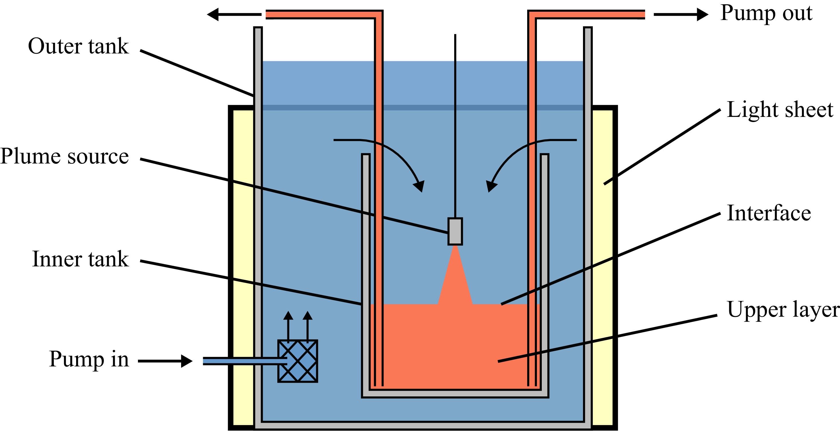
In this study, we examine the design and operation of mechanical displacement ventilation. In this ventilation strategy, fresh air, which may be precooled or preheated, is supplied at a low level, and stale air is extracted at a high level. The interaction of this upward ventilation flow with thermal plumes that rise from heat sources in the space leads to a vertical stratification at steady state with a layer of warm air above a layer of cooler supply air (Linden, Lane-Serff & Smeed Reference Linden, Lane-Serff and Smeed1990). This stratification is shown schematically in the left panel of figure 1. Ideally, excess heat and contaminants are entrained into the thermal plumes and transported into the upper layer, where they are extracted by ventilation. As a result, the occupants of the lower layer are surrounded by clean supply air (Linden Reference Linden1999; Bolster & Linden Reference Bolster and Linden2009). The height of the lower layer increases as the ventilation rate increases, leading to a tension between air quality and energy efficiency (Etheridge Reference Etheridge2015; Chenari et al. Reference Chenari, Dias Carrilho and Gameiro da Silva2016; Toy & Woods Reference Toy and Woods2025). Maintaining a higher interface between the layers is more energy-intensive, but the air quality will be poor if the interface is too low. The pragmatic design principle for most buildings is that the interface depth should be as low as possible without reaching the occupants.
In a previous study, we explored how the steady-state depth of the interface is controlled by the non-dimensional number,
 $\mu = Q_H/Q_V$
, which represents the ratio of the volume flux
 $\pi Q_H$
of a hypothetical thermal plume at the height of the ceiling associated with the heat flux , and the ventilation volume flux,
 $\pi Q_V$
(Toy & Woods Reference Toy and Woods2025). For a single heat source producing a Boussinesq plume in a uniform ambient,
 $\mu$
can be expressed as
 \begin{align} \mu = \frac {\lambda F^{1/3}H^{5/3}}{Q_V} , \end{align}
where
 $\lambda = ( {6\alpha }/{5} ) ({9\alpha }/{10} )^{1/3}$
is an empirical constant related to the entrainment coefficient
 $\alpha$
for the plume (Morton, Taylor & Turner Reference Morton, Taylor and Turner1956),
 $\pi F$
is the buoyancy flux from the heat source and
 $H$
is the distance between the heat source and the ceiling. If the ventilation is relatively weak,
 $\mu \gtrsim 2$
, the system is under-ventilated, and the distance between the heat source and interface,
 $h$
, is given approximately by
 $h/H = \mu ^{-3/5}$
(Toy & Woods Reference Toy and Woods2025). From (1.1), we observe that
 $\mu$
decreases if the source buoyancy flux or the distance to the ceiling decrease or if the ventilation rate increases. These changes lead to a permanent increase in the interface height and a decrease in the temperature of the upper layer.
Owing to transient occupancy patterns, a building may spend a significant fraction of time away from steady state as heat loads and ventilation change. Understanding how the system adjusts between steady states in these circumstances can be important.
Summary of simple transient flows following the definitions of Bower et al. (Reference Bower, Caulfield, Fitzgerald and Woods2008). (a) Intruding flow: the plume is relatively dense in the upper layer and collapses, to form a new intermediate layer. (b) Filling flow: the plume is relatively buoyant and fills a new layer above the original stratification.

When a single property is changed, for example the heat load or the ventilation flow, while the others remain constant, the pathway for evolution depends on the ratio
 \begin{align} \gamma = \frac {g'_{p}(h)}{g'_{u,i}}, \end{align}
where
 $g'_{p}(h)$
is the buoyancy of the plume fluid at the interface between the upper and lower layers, and
 $g'_{u, i}$
is the buoyancy of the upper layer in the initial steady state. Within the plume, the average buoyancy of the fluid decreases with the height above the source,
 $z$
, according to
 \begin{align} g^\prime _p(z) =\frac {F}{Q(z)} =\frac {F^{2/3}}{\lambda z^{5/3}}. \end{align}
Furthermore, the upper layer is approximately uniform in an under-ventilated system,
 $\mu \gtrsim 2$
(Toy & Woods Reference Toy and Woods2025). Assuming that the only significant volume flow into the upper layer is in the plume, this is equal to the volume flow extracted by the ventilation. Therefore, conservation of buoyancy over the upper layer leads to
 \begin{align} g^\prime _{u} = \frac {F}{Q_V}. \end{align}
In a steady state, the upper layer buoyancy is equal to the average buoyancy of the plume fluid at the interface, and
 $\gamma = 1$
.
Following a disturbance, the buoyancy of the upper layer,
 $g^\prime _{u}$
, does not change immediately. However, from (1.3), we see that variations in the source buoyancy flux or the distance between the source and the interface change the buoyancy of the plume fluid. When the buoyancy of the plume at the interface decreases, it follows that
 $\gamma \lt 1$
, and so the plume becomes negatively buoyant relative to the original upper layer. As a result, the plume fluid intrudes between the original upper and lower layers, forming a new intermediate layer (figure 1
a). This new layer grows, replacing the original upper layer, which is extracted by the high-level ventilation, leading to a new two-layer steady state. When the buoyancy of the plume increases, it follows that
 $\gamma \gt 1$
, and so the plume rises to the ceiling and forms a new buoyant layer above the original stratification (figure 1
b). This filling front descends, eventually replacing the original upper layer, which is entrained into the plume. Again, a two-layer stratification is re-established in the final steady state.
Qualitatively, the evolution of these simple transients is consistent with the intruding and filling flows described by Bower et al. (Reference Bower, Caulfield, Fitzgerald and Woods2008) following a change in the strength of a heat source in a naturally ventilated enclosure. However, in natural ventilation, the steady-state interface height is independent of the buoyancy flux from the heat source (Linden et al. Reference Linden, Lane-Serff and Smeed1990; Bolster, Maillard & Linden Reference Bolster, Maillard and Linden2008; Bower et al. Reference Bower, Caulfield, Fitzgerald and Woods2008). In contrast, in mechanical ventilation, variations in the heat load lead to permanent changes in the equilibrium interface height. As a result, if a particular interface height is required following a change in the heat load, then with mechanical ventilation this may require a change in the ventilation rate. Simultaneous changes to the buoyancy flux and ventilation rate can lead to more complex transient flows: indeed, owing to the different time scale of response of the plume to changes in the buoyancy flux and in the ventilation rate, the transient may involve a transition between the intruding and filling modes.
The purpose of this paper is to explore these different transient flow processes by combining new laboratory experiments and quantitative models, thereby building insight into the nonlinear evolution of the system subject to a range of changes in the forcing. Such modelling provides fundamental insight into the processes and identifies the key values of the dimensionless parameters which control the flows, thereby complementing more detailed numerical simulations (e.g. Yang et al. Reference Yang, Ng, Chong, Verzicco and Lohse2022).
The structure of this paper is as follows. In § 2, we describe our experimental model for displacement ventilation. Next, in § 3, we explore transient flows which result from a step change in the buoyancy flux or ventilation rate while the other is held constant. Then, in § 4, we extend the discussion to describe composite transient flows where the buoyancy flux and ventilation rate change simultaneously. In § 5, we describe and test our model for these flows with a series of new experimental observations. We conclude by discussing the implications for the design and control of displacement ventilation.
2. Experimental model of displacement ventilation
We performed a series of analogue laboratory experiments to model the transient evolution of the flow following disturbances to the heat source or ventilation flow. The experiments were performed in an inverted geometry with dense salt solutions as a proxy for warm air in a real room. Due to the small magnitude of density differences, the flow is Boussinesq, and inverting the geometry will have no significant impact on the dynamics of the experiment. This style of analogue modelling has been adopted in many earlier research papers, and by running the experiments in the same flow regime as relevant to air flows in buildings, by selecting appropriate Reynolds and Rayleigh numbers, the overall flow properties of the small-scale water-bath models have been shown to be comparable to those of large-scale airflows in buildings (Lane-Serff Reference Lane-Serff1989; Savardekar Reference Savardekar1990).
To this end, a Perspex tank, with internal dimensions 0.25
 $\times$
0.25
 $\times$
0.30 m or 0.50
 $\times$
0.50
 $\times$
0.65 m, was used to model the interior of a room. The tank was submerged in a larger tank representing the exterior. Fluid was withdrawn from the base of the model room using a peristaltic pump, and the open top allowed fluid to flow freely into the model room from the larger tank. This represents a distributed source of ventilation supply air. As an analogue model for the convective flow from an internal source of heat, a plume was created by pumping a dense salt solution into a nozzle at the top of the model room. The design of the nozzle produces a turbulent plume with a relatively small source volume and momentum flux. Inside the nozzle, the salt solution is forced through a narrow inlet into a larger cylindrical chamber, then discharged through a fine mesh at the nozzle exit (5 mm diameter). The expansion into the chamber establishes a turbulent flow within the chamber and, consequently a turbulent flow at the exit with an approximately uniform velocity profile (see Hunt & Linden Reference Hunt and Linden2001). This experimental set-up is shown schematically in figure 2.
Schematic illustrating the experimental set-up. A small open-topped tank is submerged in a larger tank of fresh water. Fluid is withdrawn from the base of the tank through multiple openings using a pump, while the open top allows for uniform inflow. A suspended plume source is supplied with a dense saltwater solution that has been dyed, and a two-layer stratification is established and photographed using a DSLR camera placed approximately 5 m from the tank. The figure is reproduced from Toy & Woods (Reference Toy and Woods2025) with permission.

In a typical experiment, the pumps driving the ventilation and plume flows were turned on, and the system was run for 5–10 ventilation time scales, so that the system would approach a steady state. Meanwhile, the outer tank was continuously refilled to replace the ventilated fluid. Next, a change was made to the system, and the transient began.
To change the ventilation volume flux, we used a MATLAB script to adjust the speed of the peristaltic pump according to a set of empirical calibrations, obtained by directly measuring the volume of fluid pumped over 300 s for each pump speed. To change the source buoyancy flux, we prepared two salt solutions of different densities, using one to establish the initial steady state and then switching to the other to initiate the transient. The switch was performed by placing the inlet pipe inside a small beaker of the starting salt solution and submerging both the beaker and the inlet pipe in the larger reservoir of the second solution. Because the volume of the first solution was less than 0.25 % of the volume of the second, this procedure had negligible impact on the density of the second salt solution. Together with axial dispersion within the inlet pipe, this switch produced a short transition region between the two salinities. The time scale for the mixed fluid to be discharged from the plume source was of order one second; however, as this is shorter than the plume travel time from source to ceiling, the adjustment of the plume salinity can be considered negligible in these experiments. The vertical position of the buoyancy source was adjusted using a motorised vertical traverse, and the horizontal position was adjusted by sliding the plume source to pre-marked locations to ensure reproducible placement.
The transient evolution of the flow was visualised by adding various colours of dye to the plume and recording the evolution with a Nikon D3500 DSLR camera fitted with a 80 mm lens, set to f/11, ISO 400 and with an exposure time of 1/50 s. Because the dye is salt based, the dissolution of the dye has a similar effect on the fluid density as the dissolution of salt. Therefore, we needed to calibrate the total density of the dyed plume to ensure that the dye did not significantly affect the flow.
A quantitative dye attenuation technique was also used to examine the flow. A light sheet was placed behind the tank to provide uniform illumination. Light passing through the tank will be partially absorbed by regions of dyed fluid, which changes the pixel intensity measured by the sensor in the camera. When dyed fluid mixes with clear fluid, the dye is diluted and will absorb less light. We can convert the measured pixel intensity to the line-of-sight average dye concentration using a set of empirical calibration curves. Then, assuming that the same processes mix dye and salt, the density distribution in the tank can be calculated. The camera was positioned far back from the tank (
 $\gtrsim 5$
m) and focused on the centre of the model room close to the interface to minimise parallax error. This arrangement means the line-of-sight average dye concentration will be close to the horizontal depth-averaged concentration. Care was taken to ensure the highest concentration was within the approximately linear portion of the calibration curve relating dye concentration to pixel intensity in order to minimise the uncertainty in the measurements.
In these experiments, which use a single colour of dye, we choose to define the interface between the upper and lower layers by the average height of the contour where the light attenuation is 10 % of the maximum. Further details of this approach have been presented by Toy & Woods (Reference Toy and Woods2025). We note that, in steady state, this approach is consistent with the location of the largest gradient in light intensity. However, there is more uncertainty during transient flows where significant gradients can develop over a large part of the upper layer.
3. Transient flows from changes to either the buoyancy flux or the ventilation rate
In this section, we explore the effect of a sudden change in the ventilation volume flux,
 $\pi Q_V$
, or the source buoyancy flux,
 $\pi F$
, while holding the other constant. This extends the experiments of Bower et al. (Reference Bower, Caulfield, Fitzgerald and Woods2008) to mechanically ventilated spaces and introduces new transients associated with variations in ventilation rate, which have not previously been examined. While the transient response shares many similarities with those earlier observations, important differences arise because mechanical ventilation decouples the ventilation flow from the internal stratification. The insights developed here will also be applied to the analysis of composite transient flows in § 4.
3.1. Experimental observations of intruding flows
When the buoyancy flux from the heat source decreases, or the ventilation rate increases, the plume fluid becomes relatively dense in the original upper layer,
 $\gamma \lt 1$
, and the plume will intrude at the original interface as the system evolves towards the new steady state. Following Bower et al. (Reference Bower, Caulfield, Fitzgerald and Woods2008) we call this an intruding flow. Between the steady states, the buoyancy of the upper layer decreases, and there is a permanent increase in the interface height.
Figure 3 shows photographs from an illustrative intruding flow experiment. Initially, the system is in steady state, with the plume fluid dyed red to distinguish the upper layer (a) and lower layer (b). Between panels 1 and 2, the ventilation rate is increased while the buoyancy flux is constant, and the colour of the dye is changed to green. The flow imbalance causes the interface to rise, so the plume entrains more fluid from the lower layer (b). As a result, the buoyancy of the plume at the interface decreases. When the plume passes into the upper layer (a), negative buoyancy forces cause the flow to stall and eventually collapse, forming a fountain (panel 3). Fluid from this fountain intrudes between the original layers, filling a new intermediate layer (c). This new layer grows and replaces the original upper layer (a). The original upper layer is drained by the high-level ventilation or entrained by the fountain. Eventually, this leads to a new two-layer stratification (c and b) (panel 6).
Dye visualisation of an experiment where the ventilation rate increases, leading to an intruding flow. Panels correspond to
 $t \lt 0$
,
 $t = 0, 25, 50, 100$
and
 $175$
s,
 $\mu _i = 20$
,
 $\Delta Q_V/Q_V = 3$
and
 $H=0.25\,\text{m}$
.

Intruding flows can also be initiated by changing the source buoyancy flux. Overall, the flows are quite similar, but there are some important differences at early times. Figure 4 compares composite images of the horizontally averaged pixel intensity at each height (y-axis) as a function of time (x-axis) in the case that the plume intrudes at the interface following a decrease in the source buoyancy flux (left panel,
 $\Delta F \lt 0$
) and an increase in ventilation rate (right panel,
 $\Delta Q \gt 0$
). When the source buoyancy flux decreases, the plume is negatively buoyant in the upper layer at
 $t=0$
and immediately intrudes, filling the intermediate layer (c). In contrast, when the ventilation rate increases, the plume is neutrally buoyant in the upper layer at
 $t=0$
but becomes negatively buoyant as the interface rises and more fluid is entrained from the lower layer. This decreasing buoyancy produces the green streak in the right-hand panel of figure 4. The descending green streak shows the decrease in the height of the fountain between early times, when it reaches the ceiling, and late times, when it stalls within the intruding layer (c) once the interface has ascended a sufficient height.
Composite images showing the evolution of the stratification during intruding flows, where the colour of the plume is changed from red to green at
 $t = 0$
(vertical line). In the left panel, decreasing the heat load (
 $\mu _i = 10$
,
 $\Delta F = -4/5$
) reduces the plume buoyancy flux, causing the intruding layer (c) to form immediately. In the right panel, increasing the ventilation (
 $\mu _i = 20$
,
 $\Delta Q / Q = 3$
) raises the interface height, indirectly reducing the plume buoyancy and leading to a delay before the intrusion forms. Each panel shows the evolution over time of the region
 $0 \leqslant z \leqslant H$
(left:
 $0\lt t \lt 1700\,\text{s}$
,
 $H = 0.51\,\text{m}$
; right:
 $0\lt t \lt 250\,\text{s}$
,
 $H = 0.25\,\text{m}$
).

In both cases, the distance between the source and interface increases monotonically through the transient flow. As a result, the buoyancy of the plume fluid continuously decreases, and the intruding layer (c) is filled from the bottom, becoming stratified. Initially, the intruding layer (c) is thin, and the overshooting fountain entrains a significant volume of fluid from the original upper layer. However, as the intruding layer grows, the fountain penetrates progressively smaller distances into the original upper layer. Eventually, the top of the new intruding layer will be above the top of the fountain, so there is no penetrative entrainment of fluid from the original upper layer.
3.2. Experimental observations of filling flows
When the buoyancy flux from the heat source increases or the ventilation rate decreases, the plume fluid will become relatively buoyant in the original upper layer,
 $\gamma \gt 1$
. As a result, the plume fluid forms a new stratified layer at the ceiling, which descends from the ceiling. Following Bower et al. (Reference Bower, Caulfield, Fitzgerald and Woods2008), we call this regime a filling flow. The final steady-state interface height is lower than the original interface height, and the buoyancy of the upper layer increases.
Figure 5 shows photographs from an illustrative filling flow experiment. Initially, the system is in steady state; the upper layer (a) is dyed red, and the lower layer (b) is clear. Between panels 1 and 2, the ventilation rate is decreased, and the colour of the plume is changed to green. The flow imbalance causes the interface to fall, so the plume entrains less fluid from the lower layer (b). As a result, the plume is relatively buoyant, rises through the upper layer and spreads across the ceiling. The supply of increasingly buoyant fluid produces a stratified layer next to the ceiling (c). Over time, the stratified front descends and replaces the original upper layer (a), which is entrained into the plume. Eventually, this leads to a new two-layer stratification (c and b) in panel 6.
Dye visualisation of an experiment where the ventilation rate decreases, leading to a filling flow. Panels correspond to
 $t \lt 0$
,
 $t = 0, 12, 38, 88$
and
 $190$
s,
 $\mu _i = 3.3$
,
 $\Delta Q_V/Q_V = -0.75$
and
 $H=0.25\,\text{m}$
.

Composite image showing the evolution of the stratification during a filling flow. The colour of the plume is changed from red to green at
 $t = 0$
(vertical line). In the left panel, increasing the heat load (
 $\mu _i = 2.8$
,
 $\Delta F / F = 2.0$
) increases the plume buoyancy flux, producing a finite density step between the layers. In the right panel, decreasing the ventilation (
 $\mu _i = 3.3$
,
 $\Delta Q_V / Q_V = -0.75$
) lowers the interface, gradually increasing the plume buoyancy and generating a smooth buoyancy profile. Each panel shows the evolution over time of the region
 $0 \leqslant z \leqslant H$
, where
 $H = 0.25\,\text{m}$
(left:
 $0\lt t \lt 300\,\text{s}$
; right:
 $0\lt t \lt 500\,\text{s}$
).

Filling flows can also be initiated by changing the source buoyancy flux. Figure 6 compares composite images of the horizontally averaged pixel intensity at each height (y-axis) as a function of time (x-axis) during a filling flow which develops following an increase in the source buoyancy flux (left panel,
 $\Delta F \gt 0$
) and a decrease in ventilation rate (right panel,
 $\Delta Q_V \lt 0$
). These flows are very similar because the plume always reaches the ceiling. However, there is a small difference in the structure of the stratification. When the ventilation decreases, the plume buoyancy is initially equal to the buoyancy of the upper layer, so the buoyancy profile is continuous. In contrast, when the buoyancy flux increases, there is a finite jump in buoyancy between the filling front (c) and the original upper layer (a). This buoyancy jump inhibits turbulent mixing associated with the kinetic energy flux supplied by the plume.
The interface height decreases monotonically throughout the transient, and the new layer (c) expands. As a result, fluid in the plume reaching the ceiling is always the most buoyant fluid in the stratification and density fronts are advected downwards towards the interface in a filling-box-type process (cf. Baines & Turner Reference Baines and Turner1969; Bower et al. Reference Bower, Caulfield, Fitzgerald and Woods2008).
3.3. Delineation of intruding and filling regimes
As we described in §§ 3.1 and 3.2, the pathway for transient evolution depends on the ratio
 $\gamma = g'_{p}/g'_{u, i}$
. In the context of modelling the flow,
 $\gamma = 1$
at steady state. Changing
 $\gamma$
so that
 $0\lt \gamma \lt 1$
leads to an intruding flow and changing
 $\gamma$
so that
 $\gamma \gt 1$
leads to a filling flow.
Combining (1.2)–(1.4), if the source buoyancy flux changes in magnitude by
 $\Delta F$
, we obtain
 \begin{align} \gamma = \left ( 1+\frac {\Delta F}{F}\right )^{2/3}. \end{align}
We assume that the vertical evolution of the plume is negligible compared with the evolution of the stratification, so that the change influences the flow instantaneously at
 $t=0$
. When
 $\Delta F \lt 0$
,
 $\gamma \lt 1$
so the flow intrudes. When
 $\Delta F \gt 0$
,
 $\gamma \gt 1$
and the flow fills.
When the ventilation rate changes by
 $\Delta Q_V$
, the interface motion is monotonic and, at early times, is approximately
 \begin{align} h(t) \approx h_{i} + \frac {\Delta Q_V}{A}t. \end{align}
This increases for
 $\Delta Q_V \gt 0$
and decreasing for
 $\Delta Q_V \lt 0$
. Combining (1.2)–(1.4), this leads to
 \begin{align} \gamma \approx \left ( 1 + \frac {\Delta Q_V}{A h_{i}}t\right )^{-5/3}. \end{align}
This time, when
 $\Delta Q_V \gt 0$
,
 $\gamma \lt 1$
and the flow intrudes whereas, when
 $\Delta Q_V \lt 0$
,
 $\gamma \gt 1$
and the flow fills.
4. Composite transient flows
The transients considered in § 3 lead to a permanent change in the interface height,
 $h$
, and the buoyancy of the upper layer,
 $g^\prime _u$
. Generally, this is also true when the source buoyancy flux and ventilation rate change simultaneously. Sometimes, the changes can be complementary. For example, the intruding flow following a decrease in the buoyancy flux or an increase in the ventilation rate leads to a higher interface and reduced buoyancy in the upper layer. As a result, when these changes occur simultaneously, they reinforce each other. However, the changes can act in opposition. For example, when simultaneously increasing the ventilation rate and the buoyancy, the interface depth and buoyancy of the upper layer in the final steady state will depend on the relative magnitude of the two changes. Consequently, compensating for a change in the buoyancy flux with a particular change in the ventilation rate can lead to a constant interface height or a constant difference in temperature across the interface. Understanding these two specific limits from the more general class of changes in buoyancy and ventilation is of particular interest and is useful for controlling the system.
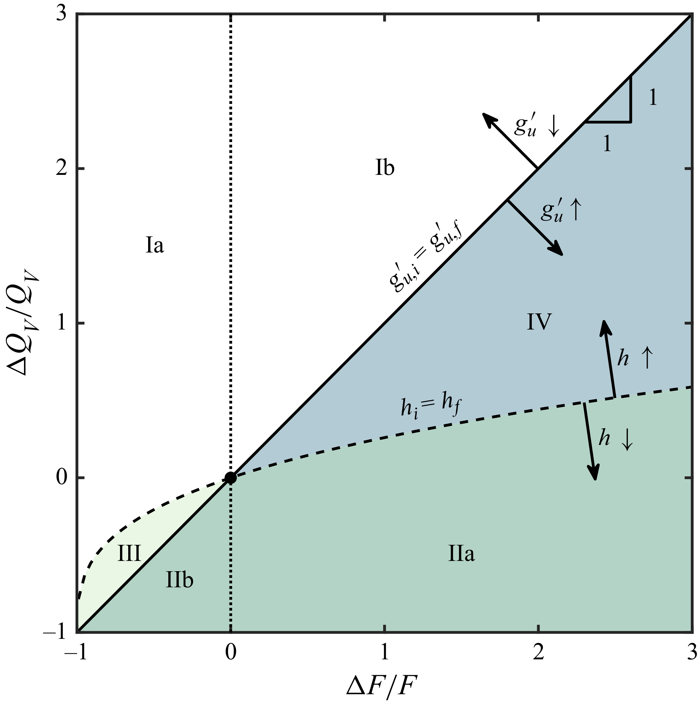
Composite transients in forced ventilation. The lines of equal interface height (dashed) and equal buoyancy (solid) segment the space into four regions based on the difference between the initial and final steady states: (I) the interface rises and buoyancy decreases, (II) the interface lowers and buoyancy increases, (III) interface lowers and buoyancy decreases, (IV) interface rises and buoyancy increases. The sign of the buoyancy change (dotted) determines whether the transient initially fills (
 $\Delta F/ F \gt 0$
) or intrudes (
 $\Delta F/ F \lt 0$
).

As described in § 1, there is usually an optimal interface height, striking a balance between air quality and energy use. As a result, following a change in the heat flux, we may change the ventilation rate to keep the interface height in the final steady state equal to the initial height,
 $h_i = h_f$
. This is equivalent to matching the strength of convection,
 $\mu$
, in the initial and final steady states. Using (1.1), for a given change in buoyancy flux,
 $\Delta F$
, the required change in ventilation rate,
 $\Delta Q_V$
, to achieve this is given by
 \begin{align} 1 + \frac {\Delta Q_V}{Q_V} = \left (1 + \frac {\Delta F}{F}\right )^{1/3}. \end{align}
This relationship is valid across the under and over-ventilated regimes because the interface height depends monotonically on
 $\mu$
(Toy & Woods Reference Toy and Woods2025).
The analogous problem in which the final buoyancy of the upper layer is equal to the initial buoyancy requires that
 $g^\prime _{u,i}=g^\prime _{u,f}$
. Assuming that the system is always under-ventilated, we can use (1.4) to show that this requires
 \begin{align} \frac {\Delta Q_V}{Q_V} = \frac {\Delta F}{F}. \end{align}
For
 $\mu \lesssim 2$
, the stratification in the upper layer develops gradients, and the average concentration is less than predicted by (1.4).
In figure 7, we show different transient flow regimes which develop as a result of a change in the buoyancy of the source (x-axis) and ventilation rate (y-axis), with the dashed line corresponding to the case in which the final equilibrium height matches the initial equilibrium height, and the solid line representing the case in which the final buoyancy of the upper layer matches the initial buoyancy. The figure segments the transient flow regimes into four classes depending on the changes between steady states. An important implication of figure 7 is that we can control the interface height or the upper layer buoyancy, but not both, because the lines only intersect at the origin.
For an arbitrary disturbance, (
 $\Delta F$
,
 $\Delta Q_V$
), the change between steady states depends on its location in figure 7 relative to the solid and dashed lines given by (4.1) and (4.2). In region (I), the interface rises, and the buoyancy of the upper layer decreases between the steady states. Conversely, in region (II), the interface falls, and the buoyancy of the upper layer increases. Regions (III) and (IV) complete the set of possible behaviours. In region (III), the interface falls, and the buoyancy decreases, while in region (IV), the interface rises and the buoyancy increases. We note that the simple transients we described in § 3 correspond to changes along the lines
 $\Delta F / F = 0$
(y-axis) and
 $\Delta Q_V/Q_V = 0$
(x-axis) and so are within regions (I) and (II).
Changing the source buoyancy flux changes
 $\gamma$
over a shorter time scale than changing the ventilation flux. As a result, the initial transient evolution only depends on the sign of
 $\Delta F$
. Therefore, we can use figure 7 to help predict the pathway for evolution.
4.1.
Decreasing source buoyancy flux,
 $\Delta F \lt 0$

A decrease in the source buoyancy flux,
 $\Delta F \lt 0$
, corresponds to points to the left of the dotted line in figure 7. Therefore,
 $\gamma \lt 1$
at
 $t=0$
and the plume initially intrudes. The interface rises in region (Ia), so
 $\gamma$
decreases, and the intrusion is maintained. The interface falls in region (III), so
 $\gamma$
is increasing. However, the initial reduction in source buoyancy flux is larger than the increase in buoyancy from the falling interface. As a result,
 $\gamma$
approaches, but is always less than, 1. Therefore, the intruding flow is maintained, but the strength of the fountain increases. Fluid from the fountain intrudes at the top of the intermediate layer, which becomes stratified. Finally, in region (IIb),
 $\gamma \lt 1$
initially, and there is an intruding flow. However,
 $\gamma$
increases and eventually, at large times,
 $\gamma \gt 1$
. As a result, the plume fluid becomes buoyant relative to the original upper layer, and the initial intruding flow switches and the plume reaches the ceiling, leading to a new upper layer which grows downward from the ceiling.
Figure 8 shows a composite image of the horizontally averaged pixel intensity at each height (y-axis) as a function of time (x-axis) during a composite transient in region (IIb). Figure 9 shows photographs of the transition. Initially, the system is in steady state, and red dye is added to the plume to distinguish the upper layer (a) and lower layer (b). A
 $t=0$
the changes
 $\Delta F/ F = -0.33$
and
 $\Delta Q_V/Q_V = -0.86$
are introduced. The decreased buoyancy flux causes the plume to intrude and fill a new intermediate layer (c) at the height where the fluid is neutrally buoyant. The flow imbalance in the upper layer causes the interface to fall, and the plume entrains less fluid from the lower layer (b). As a result, the plume becomes increasingly buoyant. The top of the fountain and the neutral buoyancy height of the plume rises through the upper layer, eventually reaching the top where it starts to fill a new layer (d) above the original upper layer. This filling layer (d) grows as the original upper layer (a) and intrusion (c) are entrained into the plume. This eventually leads to a new two-layer stratification (layers d and b).
Composite image showing the evolution of the stratification during a transient in region (IIb) over the time period
 $0 \lt t \lt 600\,\text{s}$
. The colour of the plume is changed from red to green at
 $t = 0$
(vertical line). Initially, the plume intrudes, but eventually it switches to the filling mode from above. The experimental conditions are
 $\mu _i = 5.9$
,
 $\Delta F / F = -0.33$
and
 $\Delta Q_V / Q_V = -0.86$
. The image shows the evolution over time of the region
 $0 \leqslant z \leqslant H$
, where
 $H = 0.39 \,\text{m}$
.

Dye visualisation of the transition between intruding and filling for a region (IIb) transient. The experimental conditions are
 $\mu _i = 5.9$
,
 $\Delta F/F = -0.33$
,
 $\Delta Q_V/Q_V = -0.86$
and
 $H=0.39\,\text{m}$
, panels correspond to
 $t = 40, 60, 80, 100, 120$
and
 $140$
s.

An interesting feature of figure 8 is that the band of orange fluid from the original upper layer below the intrusion is not present below the intrusions in figure 4. This band is part of the adjustment zone between the uniform lower and upper layers and is less buoyant than the fluid in the starting intrusion. In intrusions resulting from changes to a single variable, the interface rises, so the buoyancy of the plume fluid decreases, and the height where the fluid is neutrally buoyant descends through the transition zone, displacing the red fluid. In the present case, however, fluid arriving at the base of the fountain is more buoyant than the fluid already in the intruding layer, so it is filled from the top, and the band is preserved.
4.2.
Increasing source buoyancy flux,
$\Delta F \gt 0$

To the right of the dotted line in figure 7,
 $\Delta F \gt 0$
, so
 $\gamma \gt 1$
at
 $t=0$
and the plume initially reaches the ceiling and fills the space from the top. The interface falls in region (IIa), so
 $\gamma$
increases, and the plume always fills a layer next to the ceiling. The interface rises in region (IV), so
 $\gamma$
is decreasing. However, the increase in the source buoyancy flux is larger than the decrease in buoyancy from the change in interface height. Therefore, the plume remains buoyant relative to the original upper layer. Finally, in region (Ib),
 $\gamma$
decreases and, at large times,
 $\gamma \lt 1$
. As a result, the plume fluid becomes relatively dense in the original upper layer and switches from a filling flow to an intruding flow.
Composite image showing the evolution of the stratification during a transient in region (Ib) over the time period
 $0 \lt t \lt 480\,\text{s}$
. The colour of the plume is changed from red to green at
 $t = 0$
(vertical line). Initially, the plume fills the space from the ceiling, but eventually it switches, forming an intrusion. The experimental conditions are
 $\mu _i = 15$
,
 $\Delta F / F = 0.67$
and
 $\Delta Q_V / Q_V = 4.5$
. The image shows the evolution over time of the region
 $0 \leqslant z \leqslant H$
, where
 $H = 0.32\,\text{m}$
.

Dye visualisation of the transition between filling and intruding for a region (Ib) transient. The experimental conditions are
 $\mu _i = 14.9$
,
 $\Delta F/F = 0.67$
,
 $\Delta Q_V/Q_V = 4.5$
and
 $H=0.32$
, panels correspond to
 $t=120,160,200,240,280$
and
 $320$
s.

Figure 10 shows a composite image of the horizontally averaged pixel intensity at each height (y-axis) as a function of time (x-axis) during a composite transient in region (Ib). Figure 11 shows photographs of the transition. At
 $t=0$
, the changes
 $\Delta F/F = 0.67$
and
 $\Delta Q_V/Q_V = 3.4$
are introduced, and the colour of the plume is changed to green. The increased buoyancy flux leads to a filling flow (c). However, the flow imbalance into the upper layer causes the interface to rise, and the plume entrains more fluid from the lower layer (b). As a result, the plume becomes increasingly dense. The continuous change in the plume buoyancy causes the neutral height of the plume to move downward towards the interface. As a result, we see continuous intrusions of plume fluid throughout the upper layer until, eventually, the plume intrudes at the interface with the lower layer. This intrusion (d) grows while the ventilation flow extracts the higher layers (c and a). Eventually, a two-layer stratification is re-established (d and b).
In our experiments illustrating transients associated with changes to one variable (§ 3), we observe that the lateral spreading occurs on a much smaller time scale than the vertical evolution of the flow. This forms the basis of our assumption that the flow is horizontally uniform in § 5. However, in figure 11, it is seen that the edge of the box remains orange as the intrusion moves downwards. We argue that this is because as the plume fluid spreads laterally, the original orange fluid is displaced towards the edge of the tank, and as the stratification changes, it moves upwards or downwards to adjust to the evolving density gradient without mixing with the intruding flow. An analogous flow evolution was described by Li & Woods (Reference Li and Woods2023) in the case of intrusions which change the interior stratification during boundary mixing.
5. Model for the transient flow
In steady state, displacement ventilation is often modelled as two well-mixed zones connected by the plume. Bower et al. (Reference Bower, Caulfield, Fitzgerald and Woods2008) extended this approach to model filling and intruding flows by adding a third layer to the stratification. Conservation of mass and buoyancy over the three layers led to equations for the system evolution. This approach was consistent with their experimental observations because the initial change to the plume buoyancy was much larger than any variations during the subsequent evolution. However, a characteristic of the new transients identified in this paper is a continuous variation in
 $\gamma$
as the interface height adjusts. The magnitude of these variations may be larger than the initial change, leading to significant gradients in the stratification. To describe our experimental observations accurately, we, therefore, solve an advection–diffusion equation for the buoyancy profile outside the plume accounting for the vertical variations in density throughout the system.
The plume is modelled with classical plume theory (Morton et al. Reference Morton, Taylor and Turner1956). The vertical variation in the volume flux,
 $\pi Q$
, momentum flux,
 $\pi M$
, and buoyancy flux,
 $\pi F$
, are described by the conservation equations
 \begin{align} \frac {\mathop {}\!\mathrm{d} Q}{\mathop {}\!\mathrm{d} z} =2\alpha M^{1/2}, \quad \frac {\mathop {}\!\mathrm{d} M}{\mathop {}\!\mathrm{d} z} =\frac {FQ}{M}, \quad \frac {\mathop {}\!\mathrm{d} F}{\mathop {}\!\mathrm{d} z} =0, \end{align}
where
 $\alpha \approx 0.13$
is an empirically determined entrainment coefficient (cf. Baines, Turner & Campbell Reference Baines, Turner and Campbell1990; Toy & Woods Reference Toy and Woods2025) and the plume has characteristic velocity,
 $w(z) = M/Q$
, buoyancy,
 $g^\prime (z) = F/Q$
, and radius,
 $b(z) = Q/\sqrt {M}$
.
This model assumes that, to leading order, the entrainment induces a horizontal flow into the plume. In our experiments, the lack of a horizontal boundary immediately below the plume source may introduce some local deviations from this assumption. However, beyond a short zone of flow establishment, the plume is directly analogous to a classical turbulent plume above a horizontal surface. We also note that if the lateral extent of the domain becomes comparable to the plume radius, the flow is fundamentally altered and the approximation of entrainment-driven horizontal inflow is no longer valid (van Sommeren et al. Reference van Sommeren, Caulfield and Woods2012). Following Baines et al. (Reference Baines, Turner and Campbell1990), if the cross-sectional area of the room
 $\pi A$
is much larger than the cross-sectional area of the plume, the vertical velocity outside the plume,
 $v$
, is approximately
 \begin{align} v(z) = \frac {Q_V - Q(z)}{A}.\end{align}
Assuming the system is under-ventilated, advection dominates turbulent mixing outside the plume. The equation describing the evolution of the stratification is then
 \begin{align} \frac {\partial g'}{\partial t} + v \frac {\partial g'}{\partial z} = 0 , \end{align}
where
 $g'(t,z)$
is the buoyancy profile outside the plume. We assume that the plume evolves over a much shorter time scale than the surrounding stratification. Therefore, the plume equations can be integrated during each time step, assuming the surrounding stratification is steady.
5.1. Non-dimensionalisation
It is convenient to use scalings based on a hypothetical pure plume rising through a uniform layer of depth
 $z=H$
. Using the well-known solutions for a point source plume (Morton et al. Reference Morton, Taylor and Turner1956), the volume, momentum and buoyancy fluxes in this reference plume are
 \begin{align} Q_{r} = \left (\frac {6\alpha }{5}\right )\left (\frac {9\alpha }{10}\right )^{1/3} F_i^{1/3} H^{5/3},\quad M_{r} = \left (\frac {9\alpha }{10}\right )^{2/3} F_i^{2/3} H^{4/3}, \quad F_{r} = F_i, \end{align}
where
 $F_i$
is the source buoyancy flux in the initial steady state. These definitions lead to the dimensionless variables
 \begin{align} \xi = \frac {z}{H}, \quad q = \frac {Q}{Q_{r}}, \quad m = \frac {M}{M_{r}}, \quad f = \frac {F}{F_{r}} \quad \text{and} \quad \hat {g} = \frac {g^{\prime } Q_{r}}{F_{r}}. \end{align}
Equation (5.1) becomes
 \begin{align} \frac {\mathop {}\!\mathrm{d} q}{\mathop {}\!\mathrm{d} \xi } = \frac {5{\alpha }}{3} m^{1/2},\quad \frac {\mathop {}\!\mathrm{d} m}{\mathop {}\!\mathrm{d} \xi } = \frac {4}{3} \frac {fq}{m},\quad \frac {\mathop {}\!\mathrm{d} f}{\mathop {}\!\mathrm{d} \xi } = 0. \end{align}
Finally, we scale time with the filling-box time, which is defined as
 \begin{align} T_{\kern-1.5pt f} = \frac {AH}{Q_{r}(H)}. \end{align}
This is the time required to fill a room with volume
 $\pi AH$
with the volume flux
 $\pi Q_{r}$
. The dimensionless time is then
 \begin{align} \tau = \frac {t}{T_{\kern-1.5pt f}}. \end{align}
5.2. Numerical method
The ambient stratification is discretised into many uniform layers, and the plume equations are solved for each layer. At a layer interface, the volume and momentum fluxes are assumed to be continuous. Mass conservation is used to calculate the buoyancy flux of the plume in the next layer. The volume flux in the plume,
 $q$
, is used to calculate the velocity,
 $v$
, of each interface
 \begin{align} \hat {v}_{i} = q_{V} - q_{i}, \end{align}
where the subscript
 $i$
refers to the
 $i^{\text{}}$
th interface and
 $q_V$
is the dimensionless ventilation rate. The interfaces are advected, and their new position after a time step
 $\Delta \tau =0.01$
is given by
 \begin{align} \xi _{i}(\tau + \Delta \tau ) = \xi _{i}(\tau ) + \hat {v}_{i} \Delta \tau . \end{align}
This advection is driven by entrainment into the plume, so the layer depths decrease each time step. Every time step, one new layer is added next to the floor to account for fluid supplied by the ventilation, and a second new layer is added to account for fluid arriving in the plume. If the plume momentum flux is always positive, a new layer with the same composition as the plume is added next to the ceiling. Otherwise, if there is a height where the momentum flux falls to zero,
 $\xi _m$
, then we assume that the plume collapses and fluid will intrude at the neutral height,
 $\xi _n$
. This is the height where the buoyancy of the plume is equal to the buoyancy of the surrounding environment.
If penetrative entrainment is negligible, the intruding fluid will have the same composition as the plume at the neutral height, and there will be no net vertical flow in the plume. As a result,
 $q = 0$
for
 $\xi \gt \xi _n$
in (5.9) and the fluid above the intrusion is advected upwards at the speed of the ventilation flow.

Table 1 Long description
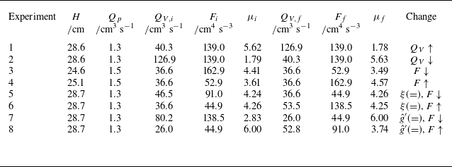
A table comparing experimental conditions across different experiments. The table has 8 rows and 10 columns. Column headers are: Experiment, H/cm, Q_p/cm3 s^-1, Q_V,i/cm3 s^-1, F_i/cm4 s^-3, μ_i, Q_V,f/cm3 s^-1, F_f/cm4 s^-3, μ_f, and Change. Row 1: Experiment 1, H 28.6, Q_p 1.3, Q_V,i 40.3, F_i 139.0, μ_i 5.62, Q_V,f 126.9, F_f 139.0, μ_f 1.78, Change Q_V↑. Row 2: Experiment 2, H 28.6, Q_p 1.3, Q_V,i 126.9, F_i 139.0, μ_i 1.79, Q_V,f 40.3, F_f 139.0, μ_f 5.63, Change Q_V↓. Row 3: Experiment 3, H 24.6, Q_p 1.5, Q_V,i 36.6, F_i 162.9, μ_i 4.41, Q_V,f 36.6, F_f 52.9, μ_f 3.49, Change F↓. Row 4: Experiment 4, H 25.1, Q_p 1.5, Q_V,i 36.6, F_i 52.9, μ_i 3.61, Q_V,f 36.6, F_f 162.9, μ_f 4.57, Change F↑. Row 5: Experiment 5, H 28.7, Q_p 1.3, Q_V,i 46.5, F_i 91.0, μ_i 4.24, Q_V,f 36.6, F_f 44.9, μ_f 4.26, Change ξ (=), F↓. Row 6: Experiment 6, H 28.7, Q_p 1.3, Q_V,i 36.6, F_i 44.9, μ_i 4.26, Q_V,f 53.5, F_f 138.5, μ_f 4.25, Change ξ (=), F↑. Row 7: Experiment 7, H 28.7, Q_p 1.3, Q_V,i 80.2, F_i 138.5, μ_i 2.83, Q_V,f 26.0, F_f 44.9, μ_f 6.00, Change g′ (=), F↓. Row 8: Experiment 8, H 28.7, Q_p 1.3, Q_V,i 26.0, F_i 44.9, μ_i 6.00, Q_V,f 52.8, F_f 91.0, μ_f 3.74, Change g′ (=), F↑.
When penetrative entrainment is significant, the composition of the plume changes and there is a net downward flow in the fountain. Dimensional arguments suggest that the total penetrative entrainment,
 $q_e$
, scales with the volume flux in the plume at the neutral buoyancy height (Kumagai Reference Kumagai1984)
 \begin{align} q_e = E q(\xi _n), \end{align}
where
 $E$
is the penetrative entrainment rate that varies with the strength of the fountain. Baines et al. (Reference Baines, Turner and Campbell1990) modelled the entrainment in a fountain to be approximately constant with height and found reasonable agreement with experiments. Adopting these modelling assumptions leads to a linearised model for the volume flux in a fountain,
 $q_f$
, between the neutral buoyancy height,
 $\xi _n$
, and the quasi-steady height of the fountain,
 $\xi _s$
 \begin{align} q_f(\xi ) = - E \left (\frac {\xi _s - \xi }{\xi _s - \xi _n}\right ) q(\xi _n), \quad \xi _n\lt \xi \lt \xi _s , \end{align}
where
 $\xi _n$
and
 $q(\xi _n)$
are found through solution of the plume equations. Additionally, we find
 $\xi _m$
, the maximum height reached by the plume before it collapses and develops a counterflow, which corresponds to the height where the momentum flux in the plume is equal to zero. The quasi-steady height of the fountain,
 $\xi _s$
, is related to the maximum height by the empirical factor
 $\xi _m/\xi _s = 1.43$
(Turner Reference Turner1966). The composition of the intruding fluid is the weighted average of the plume fluid at
 $\xi _n$
, and all of the fluid entrained between
 $\xi _n$
and
 $\xi _s$
. While this model for the fountain is idealised, it provides a reasonable and relatively simple approximation to quantify the entrainment.
5.3. Comparison with experiments
Experiments were performed to compare the measured buoyancy profile outside the plume with the predictions of the model described above. In figures 12–19, the solid black lines show the predictions of the model and the coloured lines show the measured values. The shaded region indicates the uncertainty in the measurement. The conditions for each experiment are presented in table 1.
The experiments were performed with the plume fluid dyed red and the ambient fluid clear, producing a red upper layer and a clear lower layer. The interface between the upper and lower layers was determined by the height where the light attenuation signal was
 $10\,\%$
of the maximum value in the upper layer, with the error shown by the shaded zone which bounds the regions where the light attenuation signal was 5 % and 15 %. This provides a good estimate for the height of the interface between the upper and lower layers. The vertical buoyancy profile is obtained by converting the measured light intensity of each pixel to buoyancy using a set of calibration images and assuming that the same processes mix dye and salt (see § 2). We then calculate the vertically averaged buoyancy above the interface. Again, the shaded zone shows the error and has been propagated from the uncertainty in the calibration curves. The numerical results were calculated using the same approach.
Transient evolution of the system following a change in ventilation rate. (a) Interface evolution for experiment 1, where there is an increase in ventilation; (b) average buoyancy of the upper layer during experiment 1; (c) interface evolution for experiment 2, where there is a decrease in ventilation; and (d) average buoyancy of the upper layer during experiment 2.

Figure 12 shows the transient evolution of the average buoyancy of the upper layer and the upper layer depth as a function of time following a change in the ventilation rate. In the left-hand panels (a and b), the ventilation rate has been increased,
 $\Delta Q_V/Q_V = 2.1$
, causing the plume to intrude. There is a continuous increase in the interface height and a decrease in the upper layer buoyancy between the steady states. In the right-hand panels (c and d), the ventilation rate has been decreased,
 $ \Delta Q_V / Q_V = -0.7$
, and the plume fills a new layer next to the ceiling. In this case, the interface falls, and the upper layer buoyancy increases. We see a good agreement between the experiments (blue and green lines) and the model predictions (black lines).
In figure 13, we show the full vertical buoyancy profile during the early evolution of the flow. Profiles are shown at a series of times separated by equal time intervals and offset on the x-axis by a distance proportional to the measurement time. We see a good agreement between the model and measured profile in the lower panel, where the plume fills a new layer from the ceiling. However, there is a slight discrepancy between the model and measured profile when the plume intrudes. In particular, the model predicts a sharper transition between the intruding layer and original upper layer than is observed in the model. This may be associated with turbulent mixing produced by the fountain, which occurs near the interface but is not included in the present leading-order model.
Transient evolution of the buoyancy profile outside the plume following a change in ventilation rate. (a) In experiment 1 for
 $0\leqslant \tau \leqslant 2.5$
. (b) In experiment 2 for
 $0\leqslant \tau \leqslant 5$
. Profiles are shown at a series of evenly spaced times within the interval and have been offset by a distance proportional to the measurement time. The measured interface heights are plotted with open circles.

Transient evolution of the system following a change in source buoyancy flux. (a) Interface evolution for experiment 3, where there is a decrease in buoyancy flux; (b) average buoyancy of the upper layer during experiment 3; (c) interface evolution for experiment 4, where there is an increase in buoyancy flux; and (d) average buoyancy of the upper layer in experiment 4.

Transient evolution of the buoyancy profile outside the plume following a change in source buoyancy flux. (a) In experiment 3 for
 $0\leqslant \tau \leqslant 5$
. (b) In experiment 4 for
 $0\leqslant \tau \leqslant 5$
. Profiles are shown at a series of evenly spaced times within the interval and have been offset by a distance proportional to the measurement time. The measured interface heights are plotted with open circles.

Figure 14 shows the transient evolution following a change in the source buoyancy flux. In the left-hand panels (a and b), the buoyancy flux has been decreased,
 $\Delta F/F = -0.5$
, causing the plume to intrude. The reduction in source buoyancy flux leads to a large decrease in the buoyancy of the layer, but there is only a small increase in the interface height. In the right-hand panels (c and d), the buoyancy flux has been decreased,
 $ \Delta F/F = 1.0$
, and the plume fills a new layer next to the ceiling. Again, the model predictions are consistent with the experimental observations. We show the full vertical buoyancy profile in figure 15. In this case, the intruding layer is more distinct in the measured profile than we observed for an increase in ventilation rate because there is an immediate change to the buoyancy of the plume. However, as in the last example, the measured profile is still smoother than the model, indicating that there is some mixing across the interface.
Transient evolution of the system when the change in buoyancy flux and ventilation rate lead to no change in interface height. (a) Interface evolution for experiment 5, where there is a decrease in buoyancy flux; (b) average buoyancy of the upper layer in experiment 5; (c) interface evolution for experiment 6, where there is an increase in buoyancy flux; and (d) average buoyancy of the upper layer in experiment 6.

Transient evolution of the buoyancy profile outside the plume when the change in buoyancy flux and ventilation rate lead to no change in interface height. (a) In experiment 5 for
 $0\leqslant \tau \leqslant 5$
. (b) In experiment 6 for
 $0\leqslant \tau \leqslant 2.5$
. Profiles are shown at a series of evenly spaced times within the interval and have been offset by a distance proportional to the measurement time. The measured interface heights are plotted with open circles.

Figure 16 shows the transient evolution when the change in buoyancy and ventilation rate lead to no change in the interface height (4.1). In panels (a) and (b), the buoyancy flux is decreased, which requires an increased ventilation rate. In panels (c) and (d), the buoyancy flux increases, and the ventilation rate decreases. The interface depth is constant throughout the transient in the top panels (a and c). This differs from the corresponding case with natural ventilation, where the interface will move away from the steady-state height before returning to this equilibrium height (Bower et al. Reference Bower, Caulfield, Fitzgerald and Woods2008). Again, the evolution of the full vertical buoyancy profiles shown in figure 17 are broadly consistent between the model and experiments, but the experimental profiles are somewhat smoother, perhaps owing to some of the mixing produced by the turbulence as the plume reaches the maximum height. In this case, there is a larger mismatch for the intruding profile (top panel) than when one variable is changed. A possible explanation for this is that when one variable is changed, the buoyancy of the plume decreases as the height of the interface increases. As a result, the negative buoyancy forces that oppose mixing with the original upper layer increase in magnitude as the flow evolves. In contrast, when there is no change in interface height, there is no change in the buoyancy of the plume fluid, and there is more vertical mixing.
Transient evolution of the system when the change in buoyancy flux and ventilation lead to the same upper layer buoyancy in the initial and final steady states. (a) Interface evolution for experiment 7, where there is a decrease in buoyancy flux; (b) average buoyancy of the upper layer in experiment 7; (c) interface evolution for experiment 8, where there is an increase in buoyancy flux; and (d) average buoyancy of the upper layer in experiment 8.

Transient evolution of the buoyancy profile outside the plume when the change in buoyancy flux and ventilation lead to the same upper layer buoyancy in the initial and final steady states. (a) In experiment 7 for
 $0\leqslant \tau \leqslant 5$
. (b) In experiment 8 for
 $0\leqslant \tau \leqslant 5$
. Profiles are shown at a series of evenly spaced times within the interval and have been offset by a distance proportional to the measurement time. The measured interface heights are plotted with open circles.

Figure 18 summarises the transient evolution in two experiments in which the final steady state has the same buoyancy in the upper layer as the initial steady state (4.2). In panels (a) and (b), the buoyancy flux is decreased, which requires a decrease in the ventilation rate. In panels (c) and (d), the buoyancy flux is increased, so the ventilation is also increased. We see that we have been able to match the buoyancy between the initial and final steady states. We observe an initial evolution of the upper layer buoyancy caused by the changing source buoyancy flux, followed by a return to the equilibrium height that is driven by this effect being balanced by the change in ventilation flow. Again, the models are broadly consistent with the experimental data, but there is a difference in the detailed evolution of the buoyancy profile across the layers because the experimental profiles appear smoother than the theoretical prediction.
Overall, the present model is, to a reasonable approximation, able to capture the mean density and interface height as a function of time. However, it would be of interest to develop a more detailed parametrisation of the additional mixing. This is most important for intruding flows, where the mixing may be associated with entrainment into the fountain or owing to turbulence as the flow intrudes, but the turbulent mixing associated with the interaction between the plume and ceiling could also be included (cf. Toy & Woods Reference Toy and Woods2025).
6. Application to natural ventilation
Although this paper focuses on forced ventilation, it is of interest to note that the analogous controls for naturally ventilated spaces enable the interface height or the upper layer buoyancy to remain constant following a change in the source buoyancy flux. Linden et al. (Reference Linden, Lane-Serff and Smeed1990) showed that in a naturally ventilated building the interface height,
 $h_i$
, is independent of the strength of the heat source and is a purely geometric quantity depending on the effective size of openings to the exterior,
 $A^*$
, and the distance between the heat source and the ceiling,
 $H$
, according to
 \begin{align} A^{*} = \lambda ^{3/2} \left ( \frac {h_{i}^{5}}{H-h_{i}}\right )^{1/2}, \end{align}
where
 \begin{align} \frac {1}{A^{*2}} = \frac {1}{\left (c_{l}a_{l}\right )^{2}} + \frac {1}{\left (c_{h}a_{h}\right )^{2}}, \end{align}
where, here,
 $a_{h}$
and
 $a_{l}$
denote the areas of the high and low-level openings, respectively, and the variables
 $c_{h}$
and
 $c_{l}$
are the loss coefficients associated with the flow. In natural ventilation, we often manipulate
 $A^*$
. For example, opening and closing windows is analogous to changing
 $Q_V$
in a forced system.
By analogy with § 4 for forced ventilation, there are two important lines in the regime diagram for natural ventilation: equal interface height and equal upper layer buoyancy. On the one hand, the initial and final interface heights will be equal when there is no change to the effective opening area
 \begin{align} \Delta A^{*} = 0, \end{align}
which was the situation examined by Bower et al. (Reference Bower, Caulfield, Fitzgerald and Woods2008). On the other hand, the reduced gravity of the upper layer,
 $g'_u$
, depends on the height of the interface,
 $h_{i}$
, and source buoyancy flux,
 $\pi F$
, according to
 \begin{align} g'_u = \frac {F^{2/3}}{\lambda h_{i}^{5/3}}. \end{align}
For the upper layer buoyancy to be equal in both steady states, after a change in source buoyancy flux
 $\Delta F$
, the interface height should therefore be changed by
 $\Delta h_i$
, where
 \begin{align} \left (\frac {h_{i} + \Delta h_i}{h_{i}}\right )^{5} = \left (\frac {F + \Delta F}{F}\right )^{2}. \end{align}
Using (6.1), this requires a change in the effective opening area
 $\Delta A^*$
, where
 \begin{align} \frac {A^{*}+ \Delta A^*}{A^{*}} = \left (\frac {h_{i} + \Delta h_i}{h_{i}}\right )^{5/2}\left ( \frac {H-h_{i}}{H - h_{i}-\Delta h_i}\right )^{1/2}. \end{align}
Combining (6.5) and (6.6), we obtain
 \begin{align} 1+\frac {\Delta A^{*}}{A^{*}} = \left ( 1 + \frac {\Delta F}{F}\right )\left (\frac {1-\xi _{i}}{1-\xi _{i}\left (1 + \frac {\Delta F}{F}\right )^{\frac {2}{5}}}\right )^{1/2} , \end{align}
where
 $\xi _{i} = {h_i}/{H}$
is the dimensionless interface depth in the initial steady state. Therefore, to keep the buoyancy constant, the change in opening area
 $A^*$
needed to compensate for the change in buoyancy flux also depends on the initial interface height. In figure 20, we plot (6.3) and (6.7) for
 $\xi = 0.25, 0.50$
and
 $0.75$
.
Composite transients in natural ventilation. The lines of equal interface height (dashed) and equal buoyancy (dotted, solid, dot-dashed) segment the plane into four regions: (I) the interface rises and buoyancy decreases, (II) the interface lowers and buoyancy increases, (III) the interface lowers and the buoyancy decreases, (IV) the interface rises and the buoyancy increases. Unlike in forced ventilation, the line of equal buoyancy varies with the initial conditions.

Bower et al. (Reference Bower, Caulfield, Fitzgerald and Woods2008) examined the subset of transients along the line
 $\Delta A^* / A^* = 0$
, but the present analysis suggests that a more diverse range of composite transients are also possible and figure 20 can be interpreted to understand the eventual change between steady states. It would be interesting to conduct additional experiments to examine the transient evolution between steady states.
7. Impact on energy efficiency
Displacement ventilation is often used for the efficient cooling of data centres, retail stores and offices. Although there has already been significant effort to reduce the energy demand associated with such systems, the present modelling provides an idealised framework to assess some specific opportunities for energy savings where the heating load varies over time. However, we note that in real buildings the flow dynamics may be more complex, with additional effects associated with turbulent mixing from people’s movements, as well as spatially variable heat loads.
In the idealised situation, the cool air supplied at a low level is entrained into the buoyant plumes rising above each heat source and leads to a two-layer stratification, analogous to the experiments in this paper. Typically, the design would involve the interface being above the occupants,
 $h\approx 2$
m, to ensure they remain cool.
Assuming, for simplicity, that the supply air is cooled and dehumidified by a fixed amount, the total energy required scales with the ventilation volume flux,
 $E\propto Q_V$
. As the heat load,
 $\varTheta$
, decreases, the ventilation volume flux required to manage the decreasing heat load while maintaining a fixed interface height also decreases (cf. (4.1)). The resulting potential energy savings are illustrated in figure 21, which shows that substantial reductions in cooling energy are possible at lower heat loads.
Fractional energy
 $E$
required as the heat load
 $\varTheta$
decreases from a reference value (subscript
 $R$
), using displacement ventilation, and maintaining the interface height at a fixed value.

8. Conclusions
We have analysed transient ventilation flows when there is a change in flow or buoyancy flux with a mechanical upward displacement ventilation system. Our experiments reveal that increasing either the source buoyancy flux or the ventilation rate causes a permanent change in the interface height and the buoyancy of the upper layer. However, the ventilation rate can be changed in response to changes in the strength of the heat source so that the interface height or upper layer buoyancy is unchanged.
The nature of the transient adjustment depends on whether the buoyancy of the plume at the original interface between the upper and lower layers increases or decreases relative to the upper layer. If it increases, the plume rises to the ceiling, and as it deepens, it entrains the original upper layer. In contrast, a decrease in the buoyancy of the plume leads to a new intrusion forming and ventilation of the original upper layer. However, as the flow evolves and the interface depth changes, the buoyancy of the plume at the interface, relative to the original upper layer, may change, leading to a switch from one regime to another. We observe these different regimes in our experiments.
Motivated by these observations, we develop an idealised filling-box-type model for transient flows that is broadly consistent with our experimental data. This model provides a framework for designing and controlling displacement ventilation systems in mechanically ventilated spaces
Declaration of interests
The authors report no conflicts of interest.
Appendix A. Validation of the numerical scheme
The numerical method discussed in § 5.2 models the advection of density fronts (Germeles Reference Germeles1975), and we have shown that these simulations are consistent with our experimental results. Independently, we validated the time-stepping scheme by performing simulations at successively smaller time steps,
 $\Delta \tau$
, and comparing the results with the analytical solution for the descent of the first front in a filling-box experiment. This test case is convenient because it has a closed-form solution. For this situation, performing a mass balance over the developing upper layer gives
 \begin{align} A\frac {\mathop {}\!\mathrm{d} ((h-H))}{\mathop {}\!\mathrm{d} t} = \lambda F^{1/3}h^{5/3}, \end{align}
which can be rescaled (see § 5.1), giving
 \begin{align} \frac {\mathop {}\!\mathrm{d} \xi }{\mathop {}\!\mathrm{d} \tau } = - \xi ^{5/3}. \end{align}
With the initial condition that the front starts at the top of the box
 $\xi (0) = 1$
, the solution is
 \begin{align} \xi _{analytical} = \left (1 + \frac {2}{3}\tau \right )^{-3/2}. \end{align}
We performed simulations using the numerical scheme with
 $2^{-8}\leqslant \Delta \tau \leqslant 2^{0}$
and compared these results (blue lines) with the exact solution (black line) in figure 22(a). The figure shows that the difference between the simulation and exact solution decreases as the time step decreases, although the computational cost increases significantly with smaller step sizes. For each choice of time step,
 $\Delta \tau$
, we computed the relative error
 \begin{align} \varepsilon (\Delta \tau ) = \sqrt {\frac {1}{N} \sum \limits _{n=1}^{N}\left ( \frac {\xi _{\Delta \tau }(\tau _n)-\xi _{analytical}(\tau _n)}{\xi _{analytical}(\tau _n)}\right )^2}, \end{align}
where
 $\xi _{\Delta \tau }(\tau _n)$
is the numerical solution at time
 $\tau _n$
using step size
 $\Delta \tau$
, and
 $\xi _{analytical}(\tau _n)$
is the exact solution (A3) at the same times. This provides a dimensionless measure of the relative error.
Validation of the numerical scheme. (a) Comparison of analytical solution (black line) and results of the numerical simulation (blue). (b) The relative error decreases monotonically as the step size is decreased.

The results in figure 22(b) show that the error decreases monotonically with decreasing time step, consistent with convergence of the scheme. Based on this analysis, we chose a time step of
 $\Delta \tau = 0.01$
, which provides sufficient accuracy while remaining computationally efficient. This validation gives confidence that the scheme can be reliably applied to the more complex transient problems considered in § 5.



 t<0
 t=0,25,50,100
 175
 μi=20
 ΔQV/QV=3
 H=0.25m

 t=0
 μi=10
 ΔF=−4/5
 μi=20
 ΔQ/Q=3
 0⩽z⩽H
 0
 H=0.51m
 0
 H=0.25m

 t<0
 t=0,12,38,88
 190
 μi=3.3
 ΔQV/QV=−0.75
 H=0.25m

 t=0
 μi=2.8
 ΔF/F=2.0
 μi=3.3
 ΔQV/QV=−0.75
 0⩽z⩽H
 H=0.25m
 0
 0
 ΔF/F>0
 ΔF/F<0

 0
 t=0
 μi=5.9
 ΔF/F=−0.33
 ΔQV/QV=−0.86
 0⩽z⩽H
 H=0.39m

 μi=5.9
 ΔF/F=−0.33
 ΔQV/QV=−0.86
 H=0.39m
 t=40,60,80,100,120
 140

 0
 t=0
 μi=15
 ΔF/F=0.67
 ΔQV/QV=4.5
 0⩽z⩽H
 H=0.32m

 μi=14.9
 ΔF/F=0.67
 ΔQV/QV=4.5
 H=0.32
 t=120,160,200,240,280
 320


 0⩽τ⩽2.5
 0⩽τ⩽5


 0⩽τ⩽5
 0⩽τ⩽5


 0⩽τ⩽5
 0⩽τ⩽2.5


 0⩽τ⩽5
 0⩽τ⩽5


 E
 Θ
 R


 Open access

