1. Introduction
Electron–positron (e–p) plasmas have attracted great attention as they can be found in the early universe (Gibbons, Hawking & Siklos Reference Gibbons, Hawking and Siklos1983) and in astrophysical environments, such as in active galactic nuclei (Begelman Reference Begelman, Miller and Witta1988) and in pulsar magnetospheres (Michel Reference Michel1982). Moreover, they can also be found in laboratory experiments (Berezhiani, Tskhakaya & Shukla Reference Berezhiani, Tskhakaya and Shukla1992; Greaves & Surko Reference Greaves and Surko1995). It is well known that there are no solitary-wave solutions in a cold unmagnetized e–p plasma because the electrons and positrons have the same ponderomotive force and effective mass (Berezhiani & Mahajan Reference Berezhiani and Mahajan1994). Further, Xie et al. (Reference Xie, Li, Lu and Sang2013) verified that, when the temperatures of the electrons and positrons are equal, solitary waves cannot be found in hot e–p plasmas. However, if the symmetry between electrons and positrons is broken, such as when an external magnetic field is applied (Shukla et al. Reference Shukla, Rao, Yu and Tsintsadze1986; Zank & Greaves Reference Zank and Greaves1995; Verheest & Cattaert Reference Verheest and Cattaert2004; Shukla, Eliasson & Stenflo Reference Shukla, Eliasson and Stenflo2011; Lu et al. Reference Lu, Li, Abdukerim and Xie2014), when a small fraction of ions is introduced (Berezhiani, El-Ashry & Mofiz Reference Berezhiani, El-Ashry and Mofiz1994; Berezhiani & Mahajan Reference Berezhiani and Mahajan1994, Reference Berezhiani and Mahajan1995; Popel, Vladimirov & Shukla Reference Popel, Vladimirov and Shukla1995; Mahmood & Saleem Reference Mahmood and Saleem2003), or when asymmetric temperatures of the electrons and positrons are allowed (Mahajan, Shatashvili & Berezhiani Reference Mahajan, Shatashvili and Berezhiani2009; Berezhiani, Mahajan & Shatashvili Reference Berezhiani, Mahajan and Shatashvili2010a ), it is possible for solitary-wave solutions to exist.
For the asymmetry caused by adding a fraction of ions, Berezhiani & Mahajan (Reference Berezhiani and Mahajan1995) explored the solitary-wave solutions in hot unmagnetized e–p plasmas with immobile ions. By using the long-wavelength approximation, they got a nonlinear Schrödinger equation (NLSE) of the electromagnetic field, which could capture the primary characteristics of the solitary waves, and showed the propagation of ‘heavy bullets of light’ in the plasmas. For an asymmetric temperature e–p plasma, Mahajan et al. (Reference Mahajan, Shatashvili and Berezhiani2009) applied the long-wavelength approximation to investigate the localized structure in it, and found that such a plasma can support stable wave structures with flat-topped shapes in one to three dimensions for certain parameters. They also investigated the stable localized electromagnetic pulses in asymmetric pair plasmas (Mahajan & Shatashvili Reference Mahajan and Shatashvili2008; Berezhiani et al.
Reference Berezhiani, Mahajan and Shatashvili2010a
; Berezhiani, Mahajan & Shatashvili Reference Berezhiani, Mahajan and Shatashvili2010b
). They considered the quasi-neutrality condition, i.e. long-wavelength approximation, and found the nonlinear interactions of electromagnetic waves with a primarily
 $\text{H}^{+}{-}\text{H}^{-}$
plasma containing a small impurity of high-mass ions. The standard form of the NLSE is obtained and can be solved for solitons (Mahajan & Shatashvili Reference Mahajan and Shatashvili2008). Meanwhile, Mahmood & Ur-Rehman (Reference Mahmood and Ur-Rehman2009) derived the Korteweg–de Vries equation by using the reductive perturbation method and obtained small-amplitude electrostatic solitary waves. Moreover, they also discussed the effects of ion concentration and temperature ratios of electrons and positrons on the electrostatic solitary waves. Moreover, in our previous work (Lu, Li & Xie Reference Lu, Li and Xie2013), we studied the effects of ion mobility (Lehmann & Spatschek Reference Lehmann and Spatschek2011) and positron fraction on the solitary waves with small amplitudes in a cold electron–positron–ion (e–p–i) plasma, by analytically employing the series expansion method and numerically solving the coupled equations of electromagnetic field and electrostatic potential. It was shown that the approximate analytical solutions were very consistent with the exact numerical calculations for small plasma density, while they deviated from the exact results more and more as the plasma density increased.
In the present paper, we focus on the study of the solitary waves in a hot symmetry-breaking e–p plasma, by solving the coupled simultaneous equations of the electromagnetic field and electrostatic potential as in Lu et al. (Reference Lu, Li and Xie2013), instead of invoking the long-wavelength approximation. This method enables us to deal accurately with the Poisson equation that governs the nonlinear effect due to the density perturbations. Then it allows us to look into the short-scale structures, and find some subtle structures of the electrostatic solitary waves that are omitted by employing the long-wavelength approximation. In contrast to Lu et al. (Reference Lu, Li and Xie2013), our coupled equations are based on the condition that the frequency of the electromagnetic field
 ${\it\omega}_{0}\gg 1$
, corresponding to the group velocity
 $v_{g}\simeq 1$
(here normalized quantities are used, see below). This can give large-amplitude solitary-wave solutions in an e–p–i plasma with or without a temperature. Moreover, in this paper, we consider the effects of ion motion and ion fraction on the solitary waves in both non-relativistic temperature and ultra-relativistic temperature e–p–i plasmas, and study the influence of the asymmetric temperature on the solitary waves in e–p plasmas. We hope that our research will be useful to deepen the understanding of the nonlinear properties of symmetry-breaking e–p plasmas.
The novelty of the present paper is in finding numerically the multipeak structures of solitary waves in the case of cold plasma, which are beyond the use of the long-wavelength approximation. Another novelty is the finding that the ions’ mobility can lead to slightly larger amplitude of solitary waves for relativistic high-temperature e–p plasma. Our results are quantitatively different from the work of Mahajan and co-workers. The solution of the coupled equations without using the quasi-neutrality condition means that the exact small-scale multipeak structures of the electrostatic potential can be found.
The paper is organized as follows. Section 2 reviews the theoretical model of the propagation of electromagnetic waves in hot e–p plasmas in the presence of mobile and immobile ions, and analytically presents the parameter region in which solitary waves may exist via the nonlinear dynamics method. In § 3, we display the short-scale structures of the electrostatic solitary waves by accurately solving the Poisson equation, and study the effects of asymmetric temperature, ion motion and ion ratio on the solitary-wave solutions in both non-relativistic temperature and ultra-relativistic temperature e–p plasmas. The conclusions and a discussion are given in § 4. The derivation of the coupled equations of the electromagnetic field
 $A$
and electrostatic potential
 ${\it\phi}$
are given in appendix A.
2. Theoretical model and basic formalism
The nonlinear propagation of circularly polarized electromagnetic waves in an unmagnetized and transparent hot e–p–i plasma is described by the coupled equations of
 $A$
and
 ${\it\phi}$
as well as the equation of state (for the derivation, see appendix A):
 $$\begin{eqnarray}\displaystyle & & \displaystyle 2\text{i}{\it\omega}_{0}\frac{\partial A}{\partial {\it\tau}}+\frac{1}{{\it\omega}_{0}^{2}}\left(\frac{1}{G_{0e}}+\frac{1-{\it\epsilon}}{G_{0p}}+\frac{{\it\epsilon}{\it\beta}_{i}}{G_{0i}}\right)\frac{\partial ^{2}A}{\partial {\it\xi}^{2}}\qquad \nonumber\\ \displaystyle & & \displaystyle \quad +\left[\left(\frac{1}{G_{0e}}+\frac{1-{\it\epsilon}}{G_{0p}}+\frac{{\it\epsilon}{\it\beta}_{i}}{G_{0i}}\right)-\left(\frac{1}{G_{0e}+{\it\phi}}+\frac{1-{\it\epsilon}}{G_{0p}-{\it\phi}}+\frac{{\it\epsilon}{\it\beta}_{i}}{G_{0i}-{\it\beta}_{i}{\it\phi}}\right)\right]A=0,\qquad\end{eqnarray}$$
 $$\begin{eqnarray}\displaystyle \frac{\partial ^{2}{\it\phi}}{\partial {\it\xi}^{2}} & = & \displaystyle \frac{1}{2}\left[\left(\frac{G_{e}}{G_{0e}}\right)^{2}\frac{1+|A|^{2}/G_{e}^{2}}{(1+{\it\phi}/G_{e})^{2}}-(1-{\it\epsilon})\left(\frac{G_{p}}{G_{0p}}\right)^{2}\frac{1+|A|^{2}/G_{p}^{2}}{(1-{\it\phi}/G_{p})^{2}}\right.\nonumber\\ \displaystyle & & \displaystyle -\left.{\it\epsilon}\left(\frac{G_{i}}{G_{0i}}\right)^{2}\frac{1+{\it\beta}_{i}^{2}|A|^{2}/G_{i}^{2}}{(1-{\it\beta}_{i}{\it\phi}/G_{i})^{2}}\right],\end{eqnarray}$$
 $$\begin{eqnarray}\frac{n_{{\it\alpha}}}{{\it\gamma}_{{\it\alpha}}{\it\beta}_{{\it\alpha}}T_{{\it\alpha}}\text{K}_{2}(1/({\it\beta}_{{\it\alpha}}T_{{\it\alpha}}))}\exp \left(-\frac{G_{{\it\alpha}}}{{\it\beta}_{{\it\alpha}}T_{{\it\alpha}}}\right)=\text{const.}\end{eqnarray}$$
Here
 ${\it\omega}_{0}$
is the mean frequency of the electromagnetic wave, the subscript
 ${\it\alpha}$
indicates the particle species (
 $e$
,
 $p$
and
 $i$
for electron, positron and ion, respectively),
 $G_{{\it\alpha}}=\text{K}_{3}(\cdots \,)/\text{K}_{2}(\cdots \,)$
with
 $\text{K}_{{\it\nu}}$
the modified Bessel functions,
 $G_{0{\it\alpha}}$
is the integration constant at infinity,
 ${\it\epsilon}=n_{0i}/n_{0e}$
is the ratio of unperturbed ion to electron density,
 ${\it\beta}_{{\it\alpha}}=m_{e}/m_{{\it\alpha}}$
(for electrons and positrons
 ${\it\beta}_{e}={\it\beta}_{p}=1$
, for protons
 ${\it\beta}_{i}=1/1836$
, and for the immobile case
 ${\it\beta}_{i}=0$
),
 $n_{{\it\alpha}}$
represents the particle density in the laboratory frame,
 ${\it\gamma}_{{\it\alpha}}$
is the relativistic factor, and
 $T_{{\it\alpha}}$
is the particle temperature. Here the background ion is regarded as cold, namely,
 $G_{0i}=1$
. The physical quantities are normalized as follows: time
 ${\it\omega}_{\text{e}}t$
, length
 ${\it\omega}_{e}z/c$
, potentials
 $|e|{\it\phi}/m_{e}c^{2}$
and
 $|e|\boldsymbol{A}/m_{e}c^{2}$
, electromagnetic fields
 $|e|\boldsymbol{E}/m_{e}c{\it\omega}_{\text{e}}$
and
 $|e|\boldsymbol{B}/m_{e}c{\it\omega}_{\text{e}}$
, particle temperature
 $T_{{\it\alpha}}/m_{e}c^{2}$
, density
 $n_{{\it\alpha}}/n_{0{\it\alpha}}$
, velocity
 $\boldsymbol{u}_{{\it\alpha}}/c$
, and momentum
 $\boldsymbol{p}_{{\it\alpha}}/m_{e}c$
, respectively, where
 ${\it\omega}_{\text{e}}=\sqrt{4{\rm\pi}n_{0e}e^{2}/m_{e}}$
is the electron plasma frequency, and
 $n_{0{\it\alpha}}$
is the unperturbed particle density, which satisfies an overall charge neutrality,
 $n_{0e}=n_{0p}+n_{0i}$
, in the equilibrium state of the e–p–i system.
For stationary solitary waves, we look for solutions with the following form:
 $A=a({\it\xi})\exp ((\text{i}{\it\Lambda}^{2}{\it\tau})/2{\it\omega}_{0})$
. Then (2.1) becomes
 $$\begin{eqnarray}\displaystyle & & \displaystyle \frac{1}{{\it\omega}_{0}^{2}}\left(\frac{1}{G_{0e}}+\frac{1-{\it\epsilon}}{G_{0p}}+{\it\epsilon}{\it\beta}_{i}\right)\frac{\partial ^{2}a}{\partial {\it\xi}^{2}}\qquad \nonumber\\ \displaystyle & & \displaystyle \quad +\left[\frac{1}{G_{0e}}+\frac{1-{\it\epsilon}}{G_{0p}}+{\it\epsilon}{\it\beta}_{i}-{\it\Lambda}^{2}-\left(\frac{1}{G_{0e}+{\it\phi}}+\frac{1-{\it\epsilon}}{G_{0p}-{\it\phi}}+\frac{{\it\epsilon}{\it\beta}_{i}}{1-{\it\beta}_{i}{\it\phi}}\right)\right]a=0.\qquad\end{eqnarray}$$
For non-relativistic temperatures,
 $T_{e,p}\ll 1$
and
 $G_{e,p}=1+5T_{e,p}/2$
, the equation of state (2.3) reads as
 $n_{e,p}/{\it\gamma}_{e,p}=(T_{e,p}/T_{0e,0p})^{3/2}$
, where
 $T_{0e}/T_{0p}$
is the electron/positron temperature at infinity. Once again, from (A 19), we get
 $G_{e,p}=G_{0e,0p}+5q_{e,p}T_{0e,0p}{\it\phi}/2$
. Then (2.2) can be written as
 $$\begin{eqnarray}\displaystyle \frac{\partial ^{2}{\it\phi}}{\partial {\it\xi}^{2}} & = & \displaystyle \frac{1}{2}\left[\left(1-\frac{5}{2}\frac{T_{0e}}{G_{0e}}{\it\phi}\right)^{2}\frac{1+|a|^{2}/(G_{0e}-5T_{0e}{\it\phi}/2)^{2}}{(1+{\it\phi}/G_{0e})^{2}}\right.\qquad \nonumber\\ \displaystyle & & \displaystyle -\left.(1-{\it\epsilon})\left(1+\frac{5}{2}\frac{T_{0p}}{G_{0p}}{\it\phi}\right)^{2}\frac{1+|a|^{2}/(G_{0p}+5T_{0p}{\it\phi}/2)^{2}}{(1-{\it\phi}/G_{0p})^{2}}-{\it\epsilon}\frac{1+{\it\beta}_{i}^{2}|a|^{2}}{1-{\it\beta}_{i}{\it\phi}}\right]\!.\qquad\end{eqnarray}$$
For ultra-relativistic temperatures,
 $T_{e,p}\gg 1$
and
 $G_{e,p}=4T_{e,p}$
, the equation of state (2.3) leads to
 $n_{e,p}/{\it\gamma}_{e,p}=(T_{e,p}/T_{0e,0p})^{3}=(G_{e,p}/G_{0e,0p})^{3}$
. By considering one of the important relations (A 19), we have
 $G_{e,p}=G_{0e,0p}(1-q_{e,p}{\it\phi}/G_{0e,0p})^{-1/2}$
, and then (2.2) can be reduced to
 $$\begin{eqnarray}\displaystyle \frac{\partial ^{2}{\it\phi}}{\partial {\it\xi}^{2}}=\frac{1}{2}\left[\frac{1+|a|^{2}(1+{\it\phi}/G_{0e})/G_{0e}^{2}}{(1+{\it\phi}/G_{0e})^{3}}-(1-{\it\epsilon})\frac{1+|a|^{2}(1-{\it\phi}/G_{0p})/G_{0p}^{2}}{(1-{\it\phi}/G_{0p})^{3}}-{\it\epsilon}\frac{1+{\it\beta}_{i}^{2}|a|^{2}}{1-{\it\beta}_{i}{\it\phi}}\right]\!.\hspace{-9.60004pt} & & \displaystyle \nonumber\\ \displaystyle & & \displaystyle\end{eqnarray}$$
3. Results of localized solitary-wave solutions
By solving (2.4) and (2.5), we can find the solitary-wave solutions in non-relativistic temperature plasmas. First, we discuss the nonlinear dynamics of these equations, which may predict the existence of solitary waves. From (2.4) and (2.5), we can get the fixed point
 $(a,a^{\prime },{\it\phi},{\it\phi}^{\prime })=(0,0,0,0)$
, where the prime denotes
 $\text{d}/\text{d}{\it\xi}$
. The characteristic roots of the Jacobi determinant are
 ${\it\lambda}_{1,2}^{2}={\it\Lambda}^{2}{\it\omega}_{0}^{2}/[1/G_{0e}+(1-{\it\epsilon})/G_{0p}+{\it\epsilon}{\it\beta}_{i}]$
and
 ${\it\lambda}_{3,4}^{2}=-(1/2)[(2+5T_{0e})/G_{0e}+(2+5T_{0p})(1-{\it\epsilon})/G_{0p}+{\it\epsilon}{\it\beta}_{i}]$
. In the transparent plasma,
 ${\it\omega}_{0}\gg 1$
,
 $v_{g}\simeq 1$
, it is found that, for any
 ${\it\Lambda}$
, one always has
 ${\it\lambda}_{1,2}^{2}>0$
and
 ${\it\lambda}_{3,4}^{2}<0$
, so the fixed point is a saddle centre, and solitary-wave solutions are possible in this region. The solitary-wave solutions in ultra-relativistic temperature plasmas can be found from (2.4) and (2.6). The fixed point is still
 $(a,a^{\prime },{\it\phi},{\it\phi}^{\prime })=(0,0,0,0)$
and the characteristic roots of the Jacobi determinant are
 ${\it\lambda}_{1,2}^{2}={\it\Lambda}^{2}{\it\omega}_{0}^{2}/[1/G_{0e}+(1-{\it\epsilon})/G_{0p}+{\it\epsilon}{\it\beta}_{i}]$
and
 ${\it\lambda}_{3,4}^{2}=-(1/2)[3/G_{0e}+3(1-{\it\epsilon})/G_{0p}+{\it\epsilon}{\it\beta}_{i}]$
. Similarly, for any
 ${\it\Lambda}$
, we have
 ${\it\lambda}_{1,2}^{2}>0$
and
 ${\it\lambda}_{3,4}^{2}<0$
. So the fixed point is also a saddle centre, and solitary-wave solutions are also possible in this condition.
First, we give an example of our numerical method by solving simultaneously the coupled equations of the vector potential
 $a$
and the scalar potential
 ${\it\phi}$
. For a cold e–p plasma with immobile ions, we have
 $T_{0e}=T_{0p}=0$
,
 $G_{0e}=G_{0p}=1$
and
 ${\it\beta}_{i}=0$
. Then (2.4) and (2.5) can be reduced to (10) and (11) in Berezhiani & Mahajan (Reference Berezhiani and Mahajan1994). In this case, the solitary-wave solutions of
 $a$
(dashed black line) and
 ${\it\phi}$
(solid red line) are shown in figure 1 with the parameter
 ${\it\epsilon}=0.25$
. Figure 1(a) shows the results obtained by employing the long-wavelength approximation as in Berezhiani & Mahajan (Reference Berezhiani and Mahajan1994), where the same parameter
 ${\it\Omega}=0.954629$
as in Berezhiani & Mahajan (Reference Berezhiani and Mahajan1994) is used. Figure 1(b) shows the solutions by solving the coupled equations with the same value of
 ${\it\Omega}$
as in (a) but
 ${\it\omega}_{0}=8$
and
 ${\it\Lambda}=0.090204$
are used. Comparing the results by solving coupled equations in (b) with those by the long-wavelength approximation in (a), one can see that the amplitudes and the profiles of the solitary waves are in agreement with each other and the more abundant short-scale structures of the electrostatic solitary waves appear as the oscillations in (b).
The solitary-wave solutions of vector potential
 $a$
(dashed black lines) and electrostatic potential
 ${\it\phi}$
(solid red lines) in cold e–p plasmas with immobile ions: (a) results of the long-wavelength approximation; and (b) solutions of the coupled equations. The parameters are shown in the text.

3.1. Effects of asymmetric temperature on the solitary waves in hot e–p plasmas
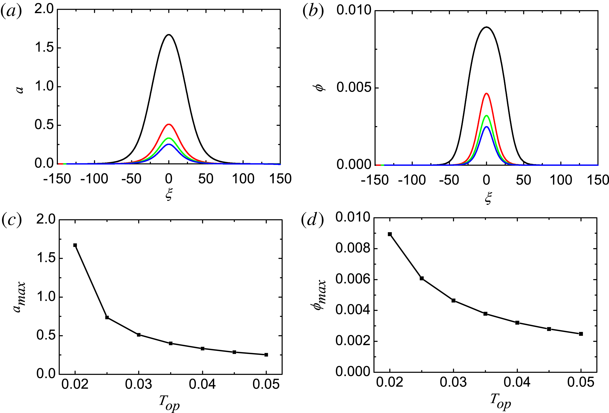
As mentioned above, when the temperatures of the electrons and positrons are the same, there are no solitary waves in pure e–p plasmas. However, asymmetric temperature e–p plasmas can sustain solitary waves. In order to study the effects of plasma temperature on the solitary waves in non-relativistic temperature e–p plasmas, we set
 ${\it\epsilon}=0$
and
 ${\it\beta}_{i}=0$
in (2.4) and (2.5). The results are plotted in figure 2 by choosing the parameters
 ${\it\omega}_{0}=8$
,
 ${\it\Lambda}^{2}=0.0002$
and
 $T_{0e}=0.01$
. Figure 2(a,b) shows the solitary waves of
 $a$
and
 ${\it\phi}$
for different positron temperatures, from top to bottom,
 $T_{0p}=0.02$
(black), 0.03 (red), 0.04 (green) and 0.05 (blue). The maximum values of
 $a_{\mathit{max}}$
and
 ${\it\phi}_{\mathit{max}}$
varying with the positron temperature are shown in figure 2(c,d), respectively. It is found that, as the positron temperature increases, the amplitudes of solitary waves decrease. If we exchange the values of
 $T_{0e}$
and
 $T_{0p}$
, the solitary waves of
 ${\it\phi}$
will become dark ones.
Solitary-wave solutions of
 $a$
and
 ${\it\phi}$
in non-relativistic temperature e–p plasmas. The parameters are chosen as
 ${\it\omega}_{0}=8$
,
 ${\it\Lambda}^{2}=0.0002$
and
 $T_{0e}=0.01$
. (a,b) Solitary-wave solutions of
 $a$
and
 ${\it\phi}$
, respectively, for different positron temperatures (from top to bottom),
 $T_{0p}=0.02$
(black), 0.03 (red), 0.04 (green) and 0.05 (blue). (c,d) Maximum values of vector potential
 $a_{\mathit{max}}$
and scalar potential
 ${\it\phi}_{\mathit{max}}$
, respectively.

For ultra-relativistic temperature e–p plasmas, we turn to solving (2.4) and (2.6), and show the results in figure 3. Similar to the non-relativistic temperature case, the amplitudes of the solitary waves decrease noticeably with increasing positron temperature, and the exchange of the temperatures of electrons and positrons gives dark solitary waves of
 ${\it\phi}$
. Furthermore, by comparing figure 3 with figure 2, we find that a high plasma temperature can support a larger-amplitude solitary wave.
Solitary-wave solutions of
 $a$
and
 ${\it\phi}$
in ultra-relativistic temperature e–p plasmas. The parameters are chosen as
 ${\it\omega}_{0}=8$
,
 ${\it\Lambda}^{2}=1\times 10^{-9}$
,
 ${\it\epsilon}=0$
,
 ${\it\beta}_{i}=0$
and
 $T_{0e}=100.0$
. (a,b) Solitary-wave solutions of
 $a$
and
 ${\it\phi}$
, respectively, for different positron temperatures (from top to bottom)
 $T_{0p}=100.5$
(black), 101.5 (red), 102.5 (green) and 103.5 (blue). (c,d) Maximum values of vector potential
 $a_{\mathit{max}}$
and scalar potential
 ${\it\phi}_{\mathit{max}}$
, respectively.

Solitary-wave solutions of
 $a$
(dashed black lines) and
 ${\it\phi}$
(solid red lines) in cold e–p plasmas with immobile ions. We fix
 $T_{0e}=T_{0p}=0$
,
 $G_{0e}=G_{0p}=1$
,
 ${\it\omega}_{0}=8$
and
 ${\it\beta}_{i}=0$
, and choose
 ${\it\Lambda}=0.012$
,
 ${\it\epsilon}=0.035$
in (a),
 ${\it\Lambda}=0.092$
,
 ${\it\epsilon}=0.27$
in (b),
 ${\it\Lambda}=0.03$
,
 ${\it\epsilon}=0.248$
in (c), and
 ${\it\Lambda}=0.09$
,
 ${\it\epsilon}=0.25$
in (d).

3.2. Effects of ion motion on the solitary waves in e–p plasmas with a fraction of ions
The solitary-wave solutions can be available in e–p plasmas with a fraction of ions, because the ions break the symmetry between electrons and positrons. For cold e–p plasmas with immobile ions, we show the solitary-wave solutions of
 $a$
(dashed black lines) and
 ${\it\phi}$
(solid red lines) in figure 4. It can be seen that short-scale structures of the electrostatic potential
 ${\it\phi}$
are clearly present – see the multipeak structures of electrostatic solitary waves in figure 4(b,d). In order to study the effects of ion motion conveniently, we choose a typical solitary wave with single-peak structure for illustration. The effects of ion motion on the solitary waves in cold e–p plasmas with mobile or immobile ions are displayed in figure 5. The parameters are chosen as
 $T_{0e}=T_{0p}=0$
,
 $G_{0e}=G_{0p}=1$
,
 ${\it\omega}_{0}=10$
,
 ${\it\Lambda}^{2}=0.00018$
and
 ${\it\epsilon}=0.15$
. Figure 5(a,b) shows the results for the immobile ions (
 ${\it\beta}_{i}=0$
) and the mobile ions (
 ${\it\beta}_{i}=1/1836$
), respectively. The solid black lines and the dashed red lines correspond to
 $a$
and
 ${\it\phi}$
, respectively. The differences in
 $a$
and
 ${\it\phi}$
between the immobile and the mobile ions are shown in figure 5(c,d). It is easy to find that the amplitudes of
 $a$
and
 ${\it\phi}$
for the mobile ions are almost the same as those for the immobile ions, namely, the ion motion has little effects on the amplitudes of the solitary waves in a cold plasma. This is because the particle effective mass
 $m_{\mathit{eff}}=m_{{\it\alpha}}G_{{\it\alpha}}(z_{{\it\alpha}})$
(Berezhiani & Mahajan Reference Berezhiani and Mahajan1995) is related to the particle temperature. When the temperatures of the electrons and positrons are zero, the effective masses of electrons and positrons are the same as their rest masses, which are much less than the ion mass. Thus the ion motion in this condition has little effect on the solitary waves.
Solitary-wave solutions of
 $a$
(solid black lines) and
 ${\it\phi}$
(dashed red lines) in cold e–p plasmas with a fraction of ions, i.e.
 $T_{0e}=T_{0p}=0$
and
 $G_{0e}=G_{0p}=1$
. Other parameters are chosen as
 ${\it\omega}_{0}=10$
,
 ${\it\Lambda}^{2}=0.00018$
and
 ${\it\epsilon}=0.15$
. (a) For immobile ions,
 ${\it\beta}_{i}=0$
, and (b) for mobile ions,
 ${\it\beta}_{i}=1/1836$
. The differences of
 $a$
between the immobile ions (solid green line) and mobile ions (dashed red line) are shown in (c), and the differences of
 ${\it\phi}$
between them are shown in (d).

For non-relativistic temperature and ultra-relativistic temperature e–p plasmas with a fraction of ions, the effects of ion motion on the solitary-wave solutions are plotted in figures 6 and 7, respectively. It is found that the ion motion has little effect on the amplitudes of solitary waves for the non-relativistic temperature case as well, because the effective masses of the electrons and positrons with low temperatures are still much less than the ion mass. For the ultra-relativistic temperature case, however, the ion motion can obviously increase the amplitudes of solitary waves, due to the fact that the effective masses of electrons and positrons with high temperatures are comparable to the mass of the ions. In this case, the effects of ion motion can no longer be neglected. Moreover, from figures 5–7, we also observe that the high temperatures of electrons and positrons can sustain larger-amplitude solitary waves.
Solitary-wave solutions of
 $a$
and
 ${\it\phi}$
in non-relativistic temperature e–p plasmas with a fraction of ions. We choose
 $T_{0e}=0.01$
,
 $T_{0p}=0.015$
,
 ${\it\omega}_{0}=10$
,
 ${\it\Lambda}^{2}=0.00008$
and
 ${\it\epsilon}=0.08$
. (a,b) Solitary-wave solutions of
 $a$
(solid black lines) and
 ${\it\phi}$
(dashed red lines) for immobile ions,
 ${\it\beta}_{i}=0$
, and mobile ions,
 ${\it\beta}_{i}=1/1836$
, respectively. The differences between the immobile ions (solid green line) and mobile ions (dashed red line) for
 $a$
are shown in (c), and for
 ${\it\phi}$
are shown in (d).

Solitary-wave solutions of
 $a$
and
 ${\it\phi}$
in ultra-relativistic temperature e–p–i plasmas with the parameters
 $T_{0e}=100$
,
 $T_{0p}=101$
,
 ${\it\omega}_{0}=10$
,
 ${\it\Lambda}^{2}=5\times 10^{-9}$
and
 ${\it\epsilon}=0.1$
. The solitary-wave solutions of
 $a$
(solid black lines) and
 ${\it\phi}$
(dashed red lines) for immobile ions,
 ${\it\beta}_{i}=0$
, and for mobile ions,
 ${\it\beta}_{i}=1/1836$
, are plotted in (a) and (b), respectively. The differences between the immobile ions (solid black lines) and mobile ions (dashed red lines) for
 $a$
and
 ${\it\phi}$
are shown in (c) and (d).

3.3. Effects of ion fraction on the solitary waves in hot e–p plasmas with ions
Now let us investigate the effects of ion fraction on the solitary-wave solutions in both non-relativistic temperature and ultra-relativistic temperature e–p plasmas with ions. The results are shown in figure 8. The maximum values of
 $a$
(a,c) and
 ${\it\phi}$
(b,d) in ultra-relativistic temperature (a,b) and non-relativistic temperature (c,d) e–p plasmas with immobile ions (green squares) and mobile ions (red circles) are shown. The parameters are chosen as
 $T_{0e}=100$
,
 $T_{0p}=102$
,
 ${\it\omega}_{0}=10$
and
 ${\it\Lambda}^{2}=1\times 10^{-9}$
in figure 8(a,b), and
 $T_{0e}=0.01$
,
 $T_{0p}=0.02$
,
 ${\it\omega}_{0}=10$
and
 ${\it\Lambda}^{2}=0.00018$
in figure 8(c,d). Here
 ${\it\epsilon}$
varies from 0.01 to 0.09,
 ${\it\beta}_{i}=0$
corresponds to immobile ions and
 ${\it\beta}_{i}=1/1836$
to mobile ions. We find that, as the ion fraction increases, the maximum values of
 $a$
and
 ${\it\phi}$
decrease. In addition, the effects of ion motion on the amplitudes of the solitary waves in the ultra-relativistic temperature case are also shown in figure 8(a,b). It is interesting to compare our results with those in Mahajan & Shatashvili (Reference Mahajan and Shatashvili2008). In that work the authors also found that the solitary-wave amplitude decreases with increasing ion fraction in cold pair plasmas contaminated by heavier immobile ions. However, their results were obtained under the condition of a non-relativistic limit. Here our theoretical model is applicable to both the relativistic and non-relativistic cases. Furthermore, as the ion fraction increases, the maximum values of
 $a$
will decrease, and when the solitary-wave amplitudes become non-relativistic, our results are almost the same as those in Mahajan & Shatashvili (Reference Mahajan and Shatashvili2008).
The maximum values of
 $a$
(a,c) and
 ${\it\phi}$
(b,d) in ultra-relativistic temperature (a,b) and non-relativistic temperature (c,d) e–p plasmas with immobile ions (green squares) and mobile ions (red circles). The parameters are given in the text.

4. Conclusion and discussion
In summary, we have investigated the solitary waves in a symmetry-breaking e–p plasma. By solving the coupled equations of
 $a$
and
 ${\it\phi}$
, we can obtain some subtle structures of the electrostatic solitary waves, such as the multipeak aspects in a cold e–p–i plasma, which are smoothed by employing the long-wavelength approximation. Moreover, the effects of asymmetric temperature, ion motion and ion fraction on the solitary waves are also studied. It is shown that the amplitudes of solitary waves decrease with the positron temperature in asymmetric temperature e–p plasmas and decrease with the ion concentration. For the effects of ion mobility on the amplitudes of solitary waves, it has little effect for the non-relativistic temperature case, but has a significant effect for the ultra-relativistic temperature case. The reason for these differences should be attributed to the effective masses of electrons and positrons. They are much less than the ion mass in the former case while being comparable in the latter case. Meanwhile electrons and positrons with high temperature can support larger-amplitude solitary waves. We also find that, as the ion fraction increases, the maximum values of
 $a$
and
 ${\it\phi}$
decrease noticeably.
It should be emphasized that our results are also helpful for understanding the nonlinear structures in pair-ion plasmas (such as
 $\text{C}_{60}^{+}{-}\text{C}_{60}^{-}$
) with a fraction of massive ions (Esfandyari-Kalejahi et al.
Reference Esfandyari-Kalejahi, Kourakis, Mehdipoor and Shukla2006; Berezhiani et al.
Reference Berezhiani, Mahajan and Shatashvili2010a
), particularly when the rest mass of the pair-ion is comparable to that of the massive ion. This means that in many cases the ion motion becomes important and it cannot be excluded in the studied problems.
Acknowledgements
This work was supported by the National Natural Science Foundation of China (NSFC) under grants nos 11475026, 11175023 and 11305010 and partially by the Fundamental Research Funds for the Central Universities (FRFCU). The computation was carried out at the HSCC of the Beijing Normal University.
Appendix A. The basic equations for the propagation of electromagnetic waves in a hot e–p–i plasma
The starting point of the propagation of electromagnetic waves in an e–p–i plasma is from the Maxwell equations. Applying the Coulomb gauge
 $\boldsymbol{{\rm\nabla}}\boldsymbol{\cdot }\boldsymbol{A}=0$
and the definitions of the vector and electrostatic potentials,
 $$\begin{eqnarray}\boldsymbol{E}=-\frac{1}{c}\frac{\partial \boldsymbol{A}}{\partial t}-\boldsymbol{{\rm\nabla}}{\it\phi},\quad \boldsymbol{B}=\boldsymbol{{\rm\nabla}}\times \boldsymbol{A},\end{eqnarray}$$
we have
 $$\begin{eqnarray}\displaystyle & \displaystyle \frac{\partial ^{2}\boldsymbol{A}}{\partial t^{2}}-c^{2}{\rm\nabla}^{2}\boldsymbol{A}+c\frac{\partial }{\partial t}(\boldsymbol{{\rm\nabla}}{\it\phi})-4{\rm\pi}c\boldsymbol{J}=0, & \displaystyle\end{eqnarray}$$
 $$\begin{eqnarray}\displaystyle & {\rm\nabla}^{2}{\it\phi}=-4{\rm\pi}{\it\rho}, & \displaystyle\end{eqnarray}$$
 $c$
is the speed of light in vacuum, and
 $$\begin{eqnarray}\displaystyle {\it\rho}=\mathop{\sum }_{{\it\alpha}}q_{{\it\alpha}}n_{{\it\alpha}}\quad \text{and}\quad \boldsymbol{J}=\mathop{\sum }_{{\it\alpha}}q_{{\it\alpha}}n_{{\it\alpha}}\boldsymbol{u}_{{\it\alpha}} & & \displaystyle\end{eqnarray}$$
are the charge and current densities, respectively. Here
 $q_{{\it\alpha}}$
refers to the electric charge for the particle species
 ${\it\alpha}$
(
 ${\it\alpha}=e,~p,~i$
for electron, positron and ion, respectively),
 $n_{{\it\alpha}}$
represents the particle density in the laboratory frame, and
 $\boldsymbol{u}_{{\it\alpha}}$
denotes the hydrodynamic velocity.
Additionally, we have the continuity equation for the particle species
 ${\it\alpha}$
,
 $$\begin{eqnarray}\displaystyle \frac{\partial n_{{\it\alpha}}}{\partial t}+\boldsymbol{{\rm\nabla}}\boldsymbol{\cdot }(n_{{\it\alpha}}\boldsymbol{u}_{{\it\alpha}})=0, & & \displaystyle\end{eqnarray}$$
and the adiabatic equation of state in the form (Berezhiani & Mahajan Reference Berezhiani and Mahajan1995; Mahajan et al. Reference Mahajan, Shatashvili and Berezhiani2009)
 $$\begin{eqnarray}\displaystyle \frac{n_{{\it\alpha}}z_{{\it\alpha}}}{{\it\gamma}_{{\it\alpha}}\text{K}_{2}(z_{{\it\alpha}})}\exp [-z_{{\it\alpha}}G_{{\it\alpha}}(z_{{\it\alpha}})]=\text{const.}, & & \displaystyle\end{eqnarray}$$
where
 $z_{{\it\alpha}}=m_{{\it\alpha}}c^{2}/T_{{\it\alpha}}$
,
 $m_{{\it\alpha}}$
and
 $T_{{\it\alpha}}$
are the rest mass and temperature for the particle species
 ${\it\alpha}$
, respectively,
 $\text{K}_{2}(z_{{\it\alpha}})$
is the modified Bessel function
 $\text{K}_{{\it\nu}}$
for
 ${\it\nu}=2$
, and
 $G_{{\it\alpha}}(z_{{\it\alpha}})=\text{K}_{3}(z_{{\it\alpha}})/\text{K}_{2}(z_{{\it\alpha}})$
. In the non-relativistic temperature limit, (A 6) becomes
 $(n_{{\it\alpha}}/{\it\gamma}_{{\it\alpha}})T_{{\it\alpha}}^{-3/2}=\text{const.}$
, and in the ultra-relativistic temperature limit it yields
 $(n_{{\it\alpha}}/{\it\gamma}_{{\it\alpha}})T_{{\it\alpha}}^{-3}=\text{const}$
.
To close the system, we should also consider the dynamics of the fluid of species
 ${\it\alpha}$
contained in the equation (Mahajan et al.
Reference Mahajan, Shatashvili and Berezhiani2009)
 $$\begin{eqnarray}\displaystyle \frac{\partial (G_{{\it\alpha}}\boldsymbol{p}_{{\it\alpha}})}{\partial t}+m_{{\it\alpha}}c^{2}\boldsymbol{{\rm\nabla}}(G_{{\it\alpha}}{\it\gamma}_{{\it\alpha}})=q_{{\it\alpha}}\boldsymbol{E}+(\boldsymbol{u}_{{\it\alpha}}\times \boldsymbol{O}_{{\it\alpha}}), & & \displaystyle\end{eqnarray}$$
where
 $\boldsymbol{E}$
and
 $\boldsymbol{B}$
are the electric and magnetic fields,
 $\boldsymbol{O}_{{\it\alpha}}=q_{{\it\alpha}}\boldsymbol{B}/c+\boldsymbol{{\rm\nabla}}\times (G_{{\it\alpha}}\boldsymbol{p}_{{\it\alpha}})$
is the generalized vorticity,
 $\boldsymbol{p}_{{\it\alpha}}={\it\gamma}_{{\it\alpha}}m_{{\it\alpha}}\boldsymbol{u}_{{\it\alpha}}$
is the hydrodynamic momentum, and
 ${\it\gamma}_{{\it\alpha}}=\sqrt{1+\boldsymbol{ p}_{{\it\alpha}}^{2}/m_{{\it\alpha}}^{2}c^{2}}$
is the relativistic factor. Notice that the relativistic thermal pressure
 $P_{{\it\alpha}}=(n_{{\it\alpha}}/{\it\gamma}_{{\it\alpha}})T_{{\it\alpha}}$
is reflected by the definition
 ${\it\gamma}_{{\it\alpha}}\boldsymbol{{\rm\nabla}}P_{{\it\alpha}}=m_{{\it\alpha}}c^{2}n_{{\it\alpha}}\boldsymbol{{\rm\nabla}}G_{{\it\alpha}}$
in (A 7).
Then the equations above can be reduced to
 $$\begin{eqnarray}\displaystyle & \displaystyle \frac{\partial ^{2}\boldsymbol{A}}{\partial t^{2}}-{\rm\nabla}^{2}\boldsymbol{A}+\frac{\partial }{\partial t}\boldsymbol{{\rm\nabla}}{\it\phi}=-\left[\frac{n_{e}\boldsymbol{p}_{e}}{{\it\gamma}_{e}}-(1-{\it\epsilon})\frac{n_{p}\boldsymbol{p}_{p}}{{\it\gamma}_{p}}-{\it\epsilon}{\it\beta}_{{\it\alpha}}\frac{n_{i}\boldsymbol{p}_{i}}{{\it\gamma}_{i}}\right], & \displaystyle\end{eqnarray}$$
 $$\begin{eqnarray}\displaystyle & \displaystyle {\rm\nabla}^{2}{\it\phi}=n_{e}-(1-{\it\epsilon})n_{p}-{\it\epsilon}n_{i}, & \displaystyle\end{eqnarray}$$
 $$\begin{eqnarray}\displaystyle & \displaystyle \frac{\partial n_{{\it\alpha}}}{\partial t}+\boldsymbol{{\rm\nabla}}\boldsymbol{\cdot }(n_{{\it\alpha}}\boldsymbol{u}_{{\it\alpha}})=0, & \displaystyle\end{eqnarray}$$
 $$\begin{eqnarray}\displaystyle & \displaystyle \frac{n_{{\it\alpha}}}{{\it\gamma}_{{\it\alpha}}{\it\beta}_{{\it\alpha}}T_{{\it\alpha}}\text{K}_{2}(1/({\it\beta}_{{\it\alpha}}T_{{\it\alpha}}))}\exp \left(-\frac{G_{{\it\alpha}}}{{\it\beta}_{{\it\alpha}}T_{{\it\alpha}}}\right)=\text{const.}, & \displaystyle\end{eqnarray}$$
 $$\begin{eqnarray}\displaystyle & \displaystyle \frac{\partial (G_{{\it\alpha}}\boldsymbol{p}_{{\it\alpha}})}{\partial t}+\frac{1}{{\it\beta}_{{\it\alpha}}}\boldsymbol{{\rm\nabla}}(G_{{\it\alpha}}{\it\gamma}_{{\it\alpha}})=-q_{{\it\alpha}}\left(\frac{\partial \boldsymbol{A}}{\partial t}+\boldsymbol{{\rm\nabla}}{\it\phi}\right), & \displaystyle\end{eqnarray}$$
 ${\it\epsilon}=n_{0i}/n_{0e}$
is the ratio of unperturbed ion to electron density,
 ${\it\gamma}_{{\it\alpha}}=\sqrt{1+{\it\beta}_{{\it\alpha}}^{2}\boldsymbol{p}_{{\it\alpha}}^{2}}$
,
 ${\it\beta}_{{\it\alpha}}$
is defined as
 $m_{e}/m_{{\it\alpha}}$
with
 ${\it\beta}_{e}={\it\beta}_{p}=1$
for electrons and positrons, and
 ${\it\beta}_{\text{i}}$
for ions, and
 $q_{{\it\alpha}}$
is the normalized electric field charge with
 $q_{e}=-1$
and
 $q_{p}=q_{i}=1$
. Note that the electromagnetic fields in (A 7) have been replaced by the potentials defined in (A 1). Furthermore, once the generalized vorticity
 $\boldsymbol{O}_{{\it\alpha}}$
is initially chosen as zero, it will be zero at any time.
Now we consider the one-dimensional propagation of circularly polarized electromagnetic waves with a slowly varying amplitude
 $A(z,t)$
along the
 $z$
axis:
 $$\begin{eqnarray}\boldsymbol{A}_{\bot }\sim {\textstyle \frac{1}{2}}(\boldsymbol{x}+\text{i}\boldsymbol{y})A(z,t)\exp (\text{i}k_{0}z-\text{i}{\it\omega}_{0}t),\end{eqnarray}$$
where
 ${\it\omega}_{0}$
and
 $k_{0}$
are the mean frequency and wavenumber, respectively. Then by integrating the transverse component of the equation of motion (A 12), we can obtain
 $$\begin{eqnarray}\boldsymbol{p}_{\bot {\it\alpha}}=\frac{q_{{\it\alpha}}\boldsymbol{A}_{\bot }}{G_{{\it\alpha}}},\end{eqnarray}$$
where the integration constant is chosen as zero owing to the assumption that the particle hydrodynamic momenta are zero at infinity where the vector potential vanishes.
For convenience, we introduce the new variables
 ${\it\xi}=z-v_{g}t$
and
 ${\it\tau}=t$
, and assume that
 $v_{g}\partial /\partial {\it\xi}\gg \partial /\partial {\it\tau}$
. Here
 $v_{g}=k_{0}/{\it\omega}_{0}$
is the group velocity of the electromagnetic wave packet. Integrating the longitudinal component of the equation of motion (A 12) and using (A 14), one can get the integral of motion
 $$\begin{eqnarray}\displaystyle \frac{1}{{\it\beta}_{{\it\alpha}}}G_{{\it\alpha}}\left[1+\frac{{\it\beta}_{{\it\alpha}}^{2}|A|^{2}}{G_{{\it\alpha}}^{2}}+{\it\beta}_{{\it\alpha}}^{2}p_{z{\it\alpha}}^{2}\right]-v_{g}G_{{\it\alpha}}p_{z{\it\alpha}}+q_{{\it\alpha}}{\it\phi}=\text{const.}, & & \displaystyle\end{eqnarray}$$
where the integration constant is set equal to
 $G_{0{\it\alpha}}/{\it\beta}_{{\it\alpha}}$
since the vector potential and plasma momentum are zero at infinity.
By considering a transparent plasma, i.e.
 ${\it\omega}_{0}\gg 1$
, corresponding to
 $v_{g}\simeq 1$
, (A 15) gives
 $$\begin{eqnarray}p_{z{\it\alpha}}=\frac{G_{{\it\alpha}}}{2{\it\beta}_{{\it\alpha}}G_{0{\it\alpha}}}\left[1+\frac{{\it\beta}_{{\it\alpha}}^{2}|A|^{2}}{G_{{\it\alpha}}^{2}}-\frac{G_{0{\it\alpha}}^{2}}{G_{{\it\alpha}}^{2}}\left(1-\frac{{\it\beta}_{{\it\alpha}}q_{{\it\alpha}}{\it\phi}}{G_{0{\it\alpha}}}\right)^{2}\right]\left(1-\frac{{\it\beta}_{{\it\alpha}}q_{{\it\alpha}}{\it\phi}}{G_{0{\it\alpha}}}\right)^{-1}\end{eqnarray}$$
and
 $$\begin{eqnarray}{\it\gamma}_{{\it\alpha}}=\frac{G_{{\it\alpha}}}{2G_{0{\it\alpha}}}\left[1+\frac{{\it\beta}_{{\it\alpha}}^{2}|A|^{2}}{G_{{\it\alpha}}^{2}}+\frac{G_{0{\it\alpha}}^{2}}{G_{{\it\alpha}}^{2}}\left(1-\frac{{\it\beta}_{{\it\alpha}}q_{{\it\alpha}}{\it\phi}}{G_{0{\it\alpha}}}\right)^{2}\right]\left(1-\frac{{\it\beta}_{{\it\alpha}}q_{{\it\alpha}}{\it\phi}}{G_{0{\it\alpha}}}\right)^{-1}.\end{eqnarray}$$
In addition, from the continuity equation (A 10) we have
 $$\begin{eqnarray}n_{{\it\alpha}}=\frac{{\it\gamma}_{{\it\alpha}}}{{\it\gamma}_{{\it\alpha}}-{\it\beta}_{{\it\alpha}}p_{z{\it\alpha}}},\end{eqnarray}$$
and then we obtain two important relations:
 $$\begin{eqnarray}\displaystyle & \displaystyle \frac{n_{{\it\alpha}}}{{\it\gamma}_{{\it\alpha}}}=\frac{G_{{\it\alpha}}}{G_{0{\it\alpha}}}\left(1-\frac{{\it\beta}_{{\it\alpha}}q_{{\it\alpha}}{\it\phi}}{G_{0{\it\alpha}}}\right)^{-1}, & \displaystyle\end{eqnarray}$$
 $$\begin{eqnarray}\displaystyle & \displaystyle {\it\gamma}_{{\it\alpha}}-p_{z{\it\alpha}}=\frac{G_{0{\it\alpha}}}{G_{{\it\alpha}}}\left(1-\frac{{\it\beta}_{{\it\alpha}}q_{{\it\alpha}}{\it\phi}}{G_{0{\it\alpha}}}\right). & \displaystyle\end{eqnarray}$$
 ${\it\alpha}$
can be written as
 $$\begin{eqnarray}n_{{\it\alpha}}=\frac{G_{{\it\alpha}}^{2}}{2G_{0{\it\alpha}}^{2}}\left(1+\frac{{\it\beta}_{{\it\alpha}}^{2}|A|^{2}}{G_{{\it\alpha}}^{2}}\right)\left(1-\frac{{\it\beta}_{{\it\alpha}}q_{{\it\alpha}}{\it\phi}}{G_{0{\it\alpha}}}\right)^{-2}+\frac{1}{2}.\end{eqnarray}$$
Finally, we get the coupled equations of the electromagnetic field
 $A$
and electrostatic potential
 ${\it\phi}$
as
 $$\begin{eqnarray}\displaystyle & & \displaystyle 2\text{i}{\it\omega}_{0}\frac{\partial A}{\partial {\it\tau}}+\frac{1}{{\it\omega}_{0}^{2}}\left(\frac{1}{G_{0e}}+\frac{1-{\it\epsilon}}{G_{0p}}+\frac{{\it\epsilon}{\it\beta}_{i}}{G_{0i}}\right)\frac{\partial ^{2}A}{\partial {\it\xi}^{2}}\nonumber\\ \displaystyle & & \displaystyle \quad +\left[\left(\frac{1}{G_{0e}}+\frac{1-{\it\epsilon}}{G_{0p}}+\frac{{\it\epsilon}{\it\beta}_{i}}{G_{0i}}\right)-\left(\frac{1}{G_{0e}+{\it\phi}}+\frac{1-{\it\epsilon}}{G_{0p}-{\it\phi}}+\frac{{\it\epsilon}{\it\beta}_{i}}{G_{0i}-{\it\beta}_{i}{\it\phi}}\right)\right]A=0,\end{eqnarray}$$
 $$\begin{eqnarray}\displaystyle \frac{\partial ^{2}{\it\phi}}{\partial {\it\xi}^{2}} & = & \displaystyle \frac{1}{2}\left[\left(\frac{G_{e}}{G_{0e}}\right)^{2}\frac{1+|A|^{2}/G_{e}^{2}}{(1+{\it\phi}/G_{e})^{2}}-(1-{\it\epsilon})\left(\frac{G_{p}}{G_{0p}}\right)^{2}\frac{1+|A|^{2}/G_{p}^{2}}{(1-{\it\phi}/G_{p})^{2}}\right.\nonumber\\ \displaystyle & & \displaystyle -\left.{\it\epsilon}\left(\frac{G_{i}}{G_{0i}}\right)^{2}\frac{1+{\it\beta}_{i}^{2}|A|^{2}/G_{i}^{2}}{(1-{\it\beta}_{i}{\it\phi}/G_{i})^{2}}\right],\end{eqnarray}$$
where the dispersion relation
 ${\it\omega}_{0}^{2}-k_{0}^{2}=1/G_{0e}+(1-{\it\epsilon})/G_{0p}+{\it\epsilon}{\it\beta}_{i}/G_{0i}$
is used.