


1 Introduction
Mixed convection occurs when both natural and forced convection processes act together to transfer heat, for example from a hot surface patch to a surrounding fluid in the presence of a wall-parallel flow. The applications of mixed convection range from small-scale problems such as cooling of industrial electronic chips (Shariat et al. Reference Shariat, Akbarinia, Nezhad and Laur2011) to large-scale flows such as ventilation of buildings or cities (De Foy et al. Reference De Foy, Varela, Molina and Molina2006; Venko et al. Reference Venko, Vidal De Ventós, Arkar and Medved2014). In general, understanding mixed-convection flow processes is more challenging than natural or forced convection due to the simultaneous and interacting effects of buoyancy and advection on flow dynamics. Probably the most well-known similarity theory dealing with mixed convection for wall-bounded flows is the Monin–Obukhov similarity theory (MOST) that provides a ‘buoyancy correction’ to the classic logarithmic laws of momentum and heat transfer over a flat homogeneous wall (Monin & Obukhov Reference Monin and Obukhov1954). Nevertheless, mixed convection in turbulent flows remains a scarcely understood process that is almost absent from most standard heat transfer textbooks (Bejan Reference Bejan1993; Bergman et al. Reference Bergman, Incropera, DeWitt and Lavine2011). The reference on the subject of turbulent mixed convection dates from 1986 (English translation two years later; Petukhov & Polyakov (Reference Petukhov and Polyakov1988)), before the emergence of modern flow simulation techniques.
Bubble and plume regimes of city-scale circulations.

Large-scale circulation around cities is an important example, among many, of a mixed-convection problem in the environment. Due to urbanization of the land surface and excess anthropogenic heat emission, urban areas are generally hotter than their surrounding rural areas, a phenomenon called the urban heat island (UHI) (Oke Reference Oke1982). Therefore, parcels of air heated over a city become lighter than their surroundings and lift up. As they rise to the top of the atmospheric boundary layer (ABL), they may be advected downstream by the background wind over the city. However, if the streamwise mean wind speed is weak, the parcels will be trapped in a thermal recirculation bubble and advected back to the city. The mechanism responsible for that thermal recirculation is the horizontal surface convergence into the city from the surroundings to replace the rising hot urban air, creating low pressure around the city. When this rising urban air encounters the inversion at the top of the ABL, it diverges outwards and is then ‘sucked down’ by this urban-fringe low-pressure zone to complete a thermal circulation cell. This is very similar to a Rayleigh–Bénard cell that is locked in place by a horizontal temperature contrast at the surface. However, under high wind conditions, streamwise advection destroys these convergence and pressure spatial patterns and transports parcels downstream of the city. While in the former weak-wind case a bubble (or dome)-shaped circulation is formed around the city, in the latter strong-wind case a plume of urban air forms and extends downwind (see sketch in figure 1). Under bubble circulation patterns, the pollutants and heat lofted from the city are constantly being recirculated into the city, deteriorating urban ventilation and environmental quality. This case is usually associated with poor air quality conditions (Klein Reference Klein2012). On the other hand, plume formation could indicate more effective removal of urban emissions and the replenishment of the city with fresh air by advection, improving environmental quality inside the city. However, in this case, the plume of air transfers heat, moisture, aerosols and other pollutants to downstream regions, deteriorating environmental quality in rural areas in the lee of cities, as well as potentially increasing the chance of precipitation in these downstream areas (Changnon Reference Changnon1979; Shepherd Reference Shepherd2005).
Previous research studies on this topic have mostly focused on the natural convection, Rayleigh–Bénard-like regime, and range from laboratory experimental investigations to analytical and numerical modelling studies (Delage & Taylor Reference Delage and Taylor1970; Hadfield, Cotton & Pielke Reference Hadfield, Cotton and Pielke1991; Ahlers, Grossmann & Lohse Reference Ahlers, Grossmann and Lohse2009; Ryu, Baik & Han Reference Ryu, Baik and Han2013; Fan et al. Reference Fan, Li, Wang and Catalano2016, Reference Fan, Li, Bejan, Wang and Yang2017; Kurbatskii & Kurbatskaya Reference Kurbatskii and Kurbatskaya2016). The forced convection limit was also considered, for example with passive scalars emitted from the urban core. These studies investigate the flow dynamics over cities under high-wind conditions, mostly focusing on how the roughness elements (buildings) influence flow and transport dynamics at smaller scales, i.e. building to neighbourhood scales (Hataya et al. Reference Hataya, Mochida, Iwata, Tabata, Yoshino and Tominaga2006; Mochida et al. Reference Mochida, Tabata, Iwata and Yoshino2008; Llaguno-Munitxa & Bou-Zeid Reference Llaguno-Munitxa and Bou-Zeid2018; Li & Bou-Zeid Reference Li and Bou-Zeid2019).
Therefore, there is still a consequential gap in our understanding of how city-scale flow transitions from a natural convection regime to a mixed convection regime and then to a forced convection regime as the wind speed gradually increases (relative to the velocity scale associated with surface heat flux to be defined later in this paper). This hinders our understanding and ability to model the full range of atmospheric conditions encountered in the real world. In particular, the following research questions remain open and will be the focus of this paper:
(i) How do different atmospheric circulation regimes scale with urban and rural surface heat fluxes and wind velocity over a city?
(ii) What are the critical values of the scaling parameters identified in (i) that characterize the flow transitions from a bubble to a plume regime?
In this paper, we bridge this gap using large-eddy simulation (LES). First, using dimensional analysis, we derive two non-dimensional parameters that are expected to control the dynamics of city-scale circulations and explain the behaviour of the ABL under various wind and UHI strengths (§ 2). Then, we verify the validity of our dimensional analysis results using LES (§§ 3 and 4). In § 5, we use these two dimensionless parameters to categorize different ABL circulations over cities as bubble, plume and transitional regimes. Finally, we discuss the implications of the findings in § 6.
2 Dimensional analysis
A primary aim of this study is to develop a general theoretical framework for assessing the relative roles of natural and forced convection in this class of problems, and how their relation modulates flow features. We start with an overview of the dimensional thermal and geometric parameters that are relevant in this problem (superscripts  $u$ and
 $r$ refer to urban and rural areas, respectively): (1) horizontal extent of the city,
 $L_{c}~(\text{m})$; (2) ABL height,
 $z_{i}~(\text{m})$; (3) and (4) momentum roughness length of the urban and rural areas,
 $z_{0,u}~(\text{m})$ and
 $z_{0,r}~(\text{m})$, respectively; (5) the spatially averaged (bulk) mean inflow speed,
 $M\;(\text{m}~\text{s}^{-1})$; and (6) and (7) buoyancy fluxes from the urban and rural surfaces,
 $(g/\unicode[STIX]{x1D703}_{0})(\overline{\unicode[STIX]{x1D703}^{\prime }w^{\prime }})_{u}$ and
 $(g/\unicode[STIX]{x1D703}_{0})(\overline{\unicode[STIX]{x1D703}^{\prime }w^{\prime }})_{r}\;(\text{m}^{2}~\text{s}^{-3})$, respectively, where
 $g=9.81\;(\text{m}~\text{s}^{-2})$ is the gravitational acceleration;
 $\unicode[STIX]{x1D703}_{0}~(\text{K})$ is a reference temperature (taken as 300 K in this paper); and
 $\unicode[STIX]{x1D703}^{\prime }$ and
 $w^{\prime }$ are the temperature and vertical velocity turbulent perturbations, respectively (their covariance is the kinematic vertical heat flux). As output, we are interested in a given velocity component (
 $u$,
 $v$ or
 $w$) that we will denote as (8)
 $u_{o}\;(\text{m}~\text{s}^{-1})$, though one could also be interested in the temperature field or other flow variables. Note that surface temperatures and thermal roughness lengths are not invoked since we use the buoyancy fluxes directly.
Using the definition of the convective velocity scale  $w_{\ast }=((g/\unicode[STIX]{x1D703}_{0})\overline{\unicode[STIX]{x1D703}^{\prime }w^{\prime }}z_{i})^{1/3}$ (Deardorff Reference Deardorff1970), a dimensionless formulation of the problem with six non-dimensional parameters (eight variables – two dimensions) can be constructed:
 $$\begin{eqnarray}\frac{u_{o}}{w_{\ast ,r}}=f\left(\frac{z_{i}}{L_{c}},\frac{z_{0,u}}{z_{0,r}},\frac{z_{0,u}}{L_{c}},\frac{M}{w_{\ast ,r}},\frac{w_{\ast ,u}}{w_{\ast ,r}}\right).\end{eqnarray}$$
The first three independent parameters on the right-hand side are related to the geometric properties of the city and rough walls; in this paper we keep them constant (at typical values) in order to focus on the dynamical effects of advection and convection encoded in the last two parameters. However, we are not suggesting that these geometric parameters, kept fixed here, are not important. Ratio  $z_{i}/L_{c}$ is the ratio of the two bulk (outer) length scales of this problem; it encodes the aspect ratio (height to horizontal scale) of the secondary circulations, and it was shown in Niino et al. (Reference Niino, Mori, Satomura and Akiba2006) to determine the type of bubble circulation patterns. Ratio
 $z_{0,u}/z_{0,r}$ is the ratio of the surface roughness length (inner) scales of the problem representing the change in surface stress (see, for example, Kimura (Reference Kimura1976), Sawai (Reference Sawai1978) and Bou-Zeid, Parlange & Meneveau (Reference Bou-Zeid, Parlange and Meneveau2007) for an illustration of roughness transition effects on the flow). Ratio
 $z_{0,u}/L_{c}$ encodes the relation between the inner and outer scales and might not be relevant if the scale separation in the turbulent spectrum is large (very high Reynolds number). Other potentially important parameters could also be formulated to account, for example, for the shape of the urban region since here we only consider square cities (circular or ellipsoidal cities are also common and previous studies indicate that this shape can have an impact on bulk circulation patterns; e.g. Fan, Li & Yin (Reference Fan, Li and Yin2018)). While future studies should investigate the impact of the geometric set-up of the problem (Sawai Reference Sawai1978), here we elect to focus on the mixed-convection dynamics.
With this focus, equation (2.1) can be simplified to
 $$\begin{eqnarray}\frac{u_{o}}{w_{\ast ,r}}=f\left(\frac{M}{w_{\ast ,r}},\frac{w_{\ast ,u}}{w_{\ast ,r}}\right).\end{eqnarray}$$
Note here that we impose a similar  $z_{i}$ for both rural and urban areas; therefore, the ratio of convective velocities can be further simplified to
 $((\overline{\unicode[STIX]{x1D703}^{\prime }w^{\prime }})_{u}/(\overline{\unicode[STIX]{x1D703}^{\prime }w^{\prime }})_{r})^{1/3}$. However, for consistency with other dimensionless parameters in (2.2), we will keep expressing the ratio as one of velocity scales. In addition, we only consider positive values of
 $w_{\ast ,r}$ and
 $w_{\ast ,u}$ corresponding to daytime convective conditions for both rural and urban areas with positive heat fluxes (where the heat flux over the urban area is higher than over the rural area due to the UHI). Potentially interesting conditions, which we do not consider here, could occur when
 $w_{\ast ,r}<0$ but
 $w_{\ast ,u}>0$ or when both are negative.
Depending on the relative magnitude of the two input dimensionless parameters in (2.2), we hypothesize (and confirm in § 4) that three scenarios will emerge.
(a) When
 $M/w_{\ast ,r}\gg w_{\ast ,u}/w_{\ast ,r}$, equation (2.2) can be reduced to $u_{o}/w_{\ast ,r}=f(M/w_{\ast ,r})$. In this scenario, the dominant factor is forced advection from the inflow, and convection due to surface heat fluxes can be neglected.
(b) When
$M/w_{\ast ,r}\ll w_{\ast ,u}/w_{\ast ,r}$, equation (2.2) can be reduced to $u_{o}/w_{\ast ,r}=f(w_{\ast ,u}/w_{\ast ,r})$. In this scenario, the ABL is close to the free (natural) convection limit, the circulations are mostly thermally driven and advection due to $M$ plays no role.(c) When
$M/w_{\ast ,r}\sim w_{\ast ,u}/w_{\ast ,r}$, the ABL experiences a mixed convection, and both input parameters on the right-hand side of (2.2) should be considered.


We should also here point out that the velocity ratios  $M/w_{\ast ,r}$ and
 $M/w_{\ast ,u}$ can each be related to its own mixed Richardson number
 $Ri=({\unicode[STIX]{x1D703}_{0}}^{-1}g\overline{\unicode[STIX]{x1D703}^{\prime }w^{\prime }})/(M^{2}(M/z_{i}))$. While this is an unconventional form that compares bulk shear effect in the denominator to buoyancy flux effect in the numerator, the physical implications are unchanged and
 $M/w_{\ast ,r}$ and
 $M/w_{\ast ,u}$ both
 ${\sim}Ri^{-1/3}$ formulated with the rural and urban flux, respectively. However, we find that our dimensionless formulation is more informative about the physics of the problem (for example in formulating these three scenarios) and we will thus not use the conventional measure of stability related to
 $Ri$.
3 Large-eddy simulations
In the current LES model, the city blocks (as groups of buildings) are resolved using the immersed boundary method (Peskin (Reference Peskin2002); the exact implementation and validation can be found in Li, Bou-Zeid & Anderson (Reference Li, Bou-Zeid and Anderson2016a) and Li et al. (Reference Li, Bou-Zeid, Anderson, Grimmond and Hultmark2016b)). To obtain the velocity and temperature fields, the spatially filtered incompressible continuity and Navier–Stokes equations using the Boussinesq approximation, in conjunction with the advection–diffusion equation for temperature, are solved as follows:
 $$\begin{eqnarray}\displaystyle & \displaystyle \frac{\unicode[STIX]{x2202}\tilde{u} _{i}}{\unicode[STIX]{x2202}x_{i}}=0, & \displaystyle\end{eqnarray}$$
 $$\begin{eqnarray}\displaystyle & \displaystyle \frac{\unicode[STIX]{x2202}\tilde{u} _{i}}{\unicode[STIX]{x2202}t}+\tilde{u} _{j}\left(\frac{\unicode[STIX]{x2202}\tilde{u} _{i}}{\unicode[STIX]{x2202}x_{j}}-\frac{\unicode[STIX]{x2202}\tilde{u} _{j}}{\unicode[STIX]{x2202}x_{i}}\right)=-\frac{1}{\unicode[STIX]{x1D70C}}\frac{\unicode[STIX]{x2202}\tilde{p}^{\ast }}{\unicode[STIX]{x2202}x_{i}}+g\frac{\tilde{\unicode[STIX]{x1D703}}^{\prime }}{\unicode[STIX]{x1D703}_{0}}\unicode[STIX]{x1D6FF}_{i3}-\frac{\unicode[STIX]{x2202}\unicode[STIX]{x1D70F}_{ij}}{\unicode[STIX]{x2202}x_{j}}+\tilde{F}_{i}+\tilde{B}_{i}, & \displaystyle\end{eqnarray}$$
 $$\begin{eqnarray}\displaystyle & \displaystyle \frac{\unicode[STIX]{x2202}\tilde{\unicode[STIX]{x1D703}}}{\unicode[STIX]{x2202}t}+\tilde{u} _{j}\frac{\unicode[STIX]{x2202}\tilde{\unicode[STIX]{x1D703}}}{\unicode[STIX]{x2202}x_{j}}=-\frac{\unicode[STIX]{x2202}\unicode[STIX]{x03C0}_{j}}{\unicode[STIX]{x2202}x_{j}}, & \displaystyle\end{eqnarray}$$
where the tilde represents filtered quantities (from now on, we omit the tilde for simplicity since all variables are filtered);  $u_{i}$ is the velocity vector in a Cartesian coordinate system (where
 $i$ and
 $j=1$, 2 or 3);
 $t$ is time;
 $\unicode[STIX]{x1D70C}$ is the air density;
 $F_{i}$ is the immersed boundary force imposed by the buildings;
 $B_{i}$ is a body force (e.g. the mean pressure gradient force driving the flow, which is needed for periodic boundary conditions but not when a domain inflow is imposed);
 $\unicode[STIX]{x1D703}$ is the potential temperature;
 $\unicode[STIX]{x03C0}_{j}$ is the subgrid-scale (SGS) heat flux;
 $\unicode[STIX]{x1D70F}_{ij}$ is the anisotropic part of the SGS stress tensor; and
 $p^{\ast }$ is the modified pressure computed as
 $$\begin{eqnarray}\tilde{p}^{\ast }=\tilde{p}+(1/3)\unicode[STIX]{x1D70C}\unicode[STIX]{x1D70E}_{kk}+(1/2)\unicode[STIX]{x1D70C}\tilde{u} _{j}\tilde{u} _{j},\end{eqnarray}$$
where  $p$ is the total pressure and
 $\unicode[STIX]{x1D70E}_{kk}$ is the trace of the full SGS stress tensor. Note that the Coriolis force is not included.
The LES model uses a scale-dependent Lagrangian dynamic model to calculate the SGS stress (Bou-Zeid, Meneveau & Parlange Reference Bou-Zeid, Meneveau and Parlange2005), and a constant SGS Prandtl number of 0.4 to infer the SGS diffusivity and compute the SGS heat flux (Li Reference Li2016). To compute the vertical derivatives on a staggered uniform grid, a second-order finite difference method is used. A pseudo-spectral differentiation scheme is adopted for horizontal derivatives (see Li et al. (Reference Li, Bou-Zeid and Anderson2016a) for details of implementation with the immersed boundary method to avoid the Gibbs phenomenon). Finally, an explicit second-order Adams–Bashforth scheme is used for the time advancement. More information and validation of the basic code can be found elsewhere (Bou-Zeid et al. Reference Bou-Zeid, Meneveau and Parlange2005; Huang & Bou-Zeid Reference Huang and Bou-Zeid2013; Shah & Bou-Zeid Reference Shah and Bou-Zeid2014; Li & Bou-Zeid Reference Li and Bou-Zeid2019). The simulations were conducted on the Cheyenne supercomputer of the National Center for Atmospheric Research (NCAR 2019).
3.1 Domain configuration and high-resolution simulation set-up
Figure 2 shows the domain set-up, where the city consists of 36 cubes each representing a full city block. The domain size is  $5~\text{km}\times 4.5~\text{km}\times 0.417~\text{km}$ in the
 $x$ (streamwise),
 $y$ (cross-stream) and
 $z$ (vertical) directions, respectively, and the corresponding baseline number of grid points is
 $288\times 256\times 48$. This leads to a grid cell size of
 $\unicode[STIX]{x0394}x=\unicode[STIX]{x0394}y=2\unicode[STIX]{x0394}z=17.4~\text{m}$. The city is a square with a side of 885 m, with one side normal to the incoming inflow velocity. Each cube is resolved using six grid points in each direction (minimum needed for an adequate representation of the flow in this code as demonstrated in Tseng, Meneveau & Parlange (Reference Tseng, Meneveau and Parlange2006)), which result in a city block size of
 $104~\text{m}\times 104~\text{m}\times 52~\text{m}$. The width of the street between two adjacent cubes is 52 m (three grid points), while the ratio of the domain height to the building height is around 8 (which is sufficient based on Li et al. (Reference Li, Bou-Zeid and Anderson2016a)). The resolution of each street or building is kept low due to computational power limitations, resulting in a reduced accuracy in representing the small-scale eddies between buildings. However, our analyses do not examine this small-scale turbulence but rather focus only on the large, city-scale eddies and flow patterns that will not be significantly affected by the resolution of each block. A grid sensitivity to demonstrate this assertion is shown in appendix A.
Simulation set-up and geometric dimensions. In addition,  $z_{0,r}=0.1~\text{ m}$ is used for rural terrain, while a roughness of 0.01 m is considered for the individual facets of the blocks. The effective
 $z_{0,u}$ of the urban terrain will be higher since it would also include the building drag resolved by the immersed boundary method.

A zero-shear-stress, no-penetration boundary condition at the top of the domain is imposed for the velocities. Additionally, a temperature inversion layer with strength of  $0.08~\text{K}~\text{m}^{-1}$ is imposed in the top 20 % of the domain. In order to ensure this inversion layer is maintained (and is not eroded by the rising thermals), at each time step, the average temperature increase of the domain below the inversion is calculated and added to the temperature above the inversion layer. That is, the inversion layer is warmed up artificially at the same rate as the other parts of the domain, leading to a constant boundary layer height. Furthermore, in order to prevent wave reflection at the top of the domain in this stably stratified inversion layer, the velocities are damped in the top 85 % of the domain using the Raleigh damping method (Klemp & Lilly Reference Klemp and Lilly1978). This vertical set-up implies that the actual boundary layer depth is
 $z_{i}=0.8L_{z}=333~\text{m}$.
The boundary conditions in the  $y$ direction are periodic for velocities and temperature in all simulations. Therefore, the domain size in the
 $y$ direction is made large enough to prevent the circulations at the lateral edges of the city from interacting with each other through the periodic boundaries (details of domain sensitivity analysis are given in appendix C). An inflow boundary condition for the velocity is imposed in the
 $x$ direction (except for the simulations where
 $M=0$ where periodic boundary conditions in
 $x$ are imposed). The boundary condition in the
 $x$ direction for temperature is an inflow for the simulations when
 $M/w_{\ast ,r}$ is larger than or of the order of
 $w_{\ast ,u}/w_{\ast ,r}$; however, it is periodic for the simulations where
 $M/w_{\ast ,r}\ll w_{\ast ,u}/w_{\ast ,r}$ (in this limit, the convection processes are dominant and the MOST is no longer valid for the rescaling of the temperature inflow that will be discussed in this section). At the end of the domain in the
 $x$ direction, when an inflow is used (we will discuss how the inflow is generated later), we impose a buffer region consisting of
 $y$–
 $z$ planes that, at each time step, interpolates/recycles the outflow solutions of velocities and temperature to the imposed/desired inflow values (Spalart Reference Spalart1988; Lund, Wu & Squires Reference Lund, Wu and Squires1998). The length of this buffer area is approximately
 $1/32$ of the domain length in the
 $x$ direction. To make sure that the wake of the flow downstream of the city (especially for high-wind simulation cases) does not perturb the interpolation in the buffer region, the city is located slightly upstream of the centre of the domain in the
 $x$ direction, at 1.8 km from the inflow boundary and at 2.315 km from the outflow boundary. The distance of the city edge to the
 $y$ boundaries is also 1.8 km. The most appropriate length scale for normalizing these geometric scales is the depth of the boundary layer (333 m).
The inflows for velocities and temperature are generated in precursor simulations with periodic boundary conditions in both  $x$ and
 $y$ directions. The surface heat flux and momentum roughness length imposed in the precursor simulations are set equal to their values over rural areas in the main simulations to represent an infinitely homogeneous upstream fetch. In order to minimize the number of precursor runs for inflow generation, for each unique value of rural heat flux, only one main inflow is generated; subsequently the inflow velocities and temperatures are rescaled to modify the inflow bulk velocity and produce simulations with a different
 $M/w_{\ast ,r}$. The details of rescaling the inflow velocity and temperature are discussed in appendix B, but we note that this rescaling will have a minimal impact on our results because (i) the inflow is allowed to evolve over a distance of approximately five times the boundary layer depth
 $(1800~\text{m}/333~\text{m})$ inside the main domain to further adjust to the upstream rural surface before it meets the city (Bou-Zeid, Meneveau & Parlange Reference Bou-Zeid, Meneveau and Parlange2004) and (ii) regardless of the rescaling results, the
 $M$ used in the analyses is the one actually attained and computed just upstream of the city in the main domain.
Recall that for all the simulations we set the momentum roughness length for rural area to 0.1 m and that of the facets of the blocks (i.e. walls, roofs and streets) to 0.01 m. In addition,  $z_{0,h}$ is taken as
 $1/10$ of the momentum roughness length to approximate rough rural surfaces for inflow rescaling (equation (B 6) in appendix B), but the value of
 $z_{0,h}$ is not needed in the wall model of the LES since we prescribe the heat flux. We impose the surface heat flux for rural
 $(H_{r}=\unicode[STIX]{x1D70C}c_{p}(\overline{\unicode[STIX]{x1D703}^{\prime }w^{\prime }})_{r})$ and urban
 $(H_{u}=\unicode[STIX]{x1D70C}c_{p}(\overline{\unicode[STIX]{x1D703}^{\prime }w^{\prime }})_{u})$ areas, with the urban area heat flux taken to be greater than the rural area heat flux to represent UHI conditions (
 $\unicode[STIX]{x1D70C}$ and
 $c_{p}$ are the density and heat capacity of the air). In addition, in the urban areas, heat fluxes are imposed on the horizontal surfaces (ground surface and roof, but not walls) of the buildings in order to represent conditions around solar noon.
3.2 Simulation scenarios and methodology
To answer the two questions on city-scale circulations overviewed in the introduction, we adopt the following methodology:
(i) To test the two scaling parameters proposed in the dimensional analysis section and the general validity of that analysis, we conduct high-resolution LES based on the set-up introduced in the previous section. These analyses help us understand how important each of the scaling parameters is under different circulation regimes ((a) to (c) in § 2), and how the dynamics of these circulations transition between the different regimes. Details and results of these simulations are discussed next and in § 4.
(ii) To propose a generalizable categorization of the circulations into bubble, transitional and plume regimes, we need a larger suite of simulations to cover the entire parameter space. Therefore, in § 5, we introduce a suite of a lower-resolution simulations that fully and finely span that parameter space for
$M/w_{\ast ,r}$ and $w_{\ast ,u}/w_{\ast ,r}$. These simulations then enable us to classify the flows into the three regimes and to identify a parameter that can a priori predict the resulting flow regime.


First we focus on testing the scaling hypothesized in (2.2). To that end, we conducted eight simulations detailed in table 1:
(a) When
$M/w_{\ast ,r}\sim w_{\ast ,u}/w_{\ast ,r}$, four simulation cases are conducted (cases 1–4 in table 1). Case 1 is the base case in this regime with $M/w_{\ast ,r}=0.96$ and $w_{\ast ,u}/w_{\ast ,r}=1.4$. Then cases 2, 3 and 4 are constructed by changing the values of $M$, $w_{\ast ,r}$ and $w_{\ast ,u}$ in order to obtain:(i) Case 2: maintain both ratios
$M/w_{\ast ,r}$ and $w_{\ast ,u}/w_{\ast ,r}$ equal to the base case but with different dimensional inputs; the results should be identical to the base case if our hypothesis is correct, and the flow is controlled only by these two dimensionless parameters.(ii) Case 3: only
$w_{\ast ,u}/w_{\ast ,r}$ is changed from the base case to illustrate that the results are different from the base case and that this ratio is consequential.(iii) Case 4: only
$M/w_{\ast ,r}$ is changed from the base case to show that the results are different from the base case and that this ratio is also consequential.
These cases allow us to show that when both dimensionless parameters are of the same order, they both impact the flow dynamics and are important to scale the problem.
(b) When
$M/w_{\ast ,r}\gg w_{\ast ,u}/w_{\ast ,r}$, we conducted two simulations (cases 5 and 6 in table 1). We consider case 5 as the base case of this limit with $M/w_{\ast ,r}=15.9$ and $w_{\ast ,u}/w_{\ast ,r}=1.4$. Case 6 is constructed by keeping $M/w_{\ast ,r}$ the same as the base case but changing $w_{\ast ,u}/w_{\ast ,r}$. The two simulation are shown to be similar to demonstrate that in this limit, $M/w_{\ast ,r}$ is the only controlling non-dimensional ratio and changes in $w_{\ast ,u}/w_{\ast ,r}$ are inconsequential.(c) Finally, the limit where
$M/w_{\ast ,r}\ll w_{\ast ,u}/w_{\ast ,r}$ is examined in cases 7 and 8 in table 1. Case 7 is the base case with $M/w_{\ast ,r}=0$ and $w_{\ast ,u}/w_{\ast ,r}=1.4$, while case 8 has the same $w_{\ast ,u}/w_{\ast ,r}$ as the base case, but $M/w_{\ast ,r}=0.1$. The results are shown to be practically identical, demonstrating that $M/w_{\ast ,r}$ is irrelevant and the ratio of the convective velocity scales dominates the dynamics in this limit of natural convection.


Simulation cases: numbers underlined and in bold are the ones that were modified from the base case for each regime.

4 Results
4.1 City-scale circulations: flow characteristics
Figure 3 depicts a pseudocolour plot of the time-averaged streamwise velocity  $\langle u\rangle _{t}$ (brackets denote time averaging; more details are provided in § 4.2) in an
 $x$–
 $z$ slice that crosses the mid-point of the city (at
 $y/L_{c}=2.5$). Three plots illustrate unambiguously the existence of the three distinct circulation regimes: (
 $a$) plume regime (case 5), (
 $b$) transitional regime between plume and bubble (case 1) and (
 $c$) bubble regime (case 7). For the plume case (from figure 3a), the flow over the city is deflected upward as it reaches the city, and then it subsides in the downstream area. The plot suggests that the city influences the flow up to three times the city height
 $(H)$. Then, above this height, the effects of the city on the flow dynamics become minimal. The flow velocity is generally slower downstream of the city, with a small recirculation zone behind the city. In the bubble case (figure 3c), two symmetric main circulations can be seen on either side of the city with comparable strengths. The horizontal distance over which each of these circulations extends is approximately equal to the city size. In addition, there are smaller and weaker secondary circulations further away from the city (both upstream and downstream of the city) with smaller horizontal scales. The flow pattern in the transitional case (figure 3b) is a fusion of the flow characteristics of the plume and bubble regimes. In this case, there is a general horizontal direction for the flow (from left to right in figure 3b); however, above the city, the velocity is mainly upward indicating that thermal convection overcomes advection and lifts the warm air parcels to produce a unique circulation around the city.
Pseudocolour plots of time-averaged normalized streamwise velocity  $\langle u\rangle$ over
 $x$–
 $z$ slices for the cases of (a) plume (case 5), (b) transitional (case 1) and (c) bubble (case 7) regimes. The inversion layer (which starts at
 $0.8L_{z}$) is excluded from the plots. The white masked area contains both city blocks (solid space) and streets (fluid space).

Figure 4 shows the pseudocolour maps of the vertical velocity in  $x$–
 $y$ slices for the bubble regime case (also averaged in time). These slices are shown for three different heights:
 $z/H=1.5$,
 $z/H=4$ and
 $z/H=5.8$. This figure reveals the three-dimensional structure of the circulations around the city. For all heights, a high vertical velocity region above the urban area can be seen. At low elevations
 $(z/H=1.5)$, there is a convergence zone above the city, while for higher elevations
 $(z/H=5.8)$ a divergence zone can be seen over the urban region. For intermediate heights
 $(z/H=4)$, the flow is less structured; however, the main circulation around the city is still very clear. For
 $z/H=1.5$, the maps of vertical velocity match the city topography, and strong upwelling thermals (red bands in figure 4a) are noted over the blocks.
Pseudocolour plots of the normalized time-averaged vertical velocity  $\langle w\rangle$ over
 $x$–
 $y$ slices, for the bubble regime (case 7), plotted for three different heights: (a)
 $1.5H\,(z/L_{c}=0.09)$, (b)
 $4H\,(z/L_{c}=0.23)$ and (c)
 $5.8H$
 $(z/L_{c}=0.34)$. The velocity is normalized by the convective velocity of rural area
 $(w_{\ast ,r})$. The lines are the streamlines of the horizontal velocity.

4.2 Spatial and time averaging
Given the spatial heterogeneity of the flow, Reynolds averaging can only be surrogated for by time averaging and we define perturbations only relative to a time average. Nevertheless, we can also spatially average any turbulent statistics over the city to identify flow structures or for other analyses. For a variable  $\unicode[STIX]{x1D711}$, the averaged value is denoted as
 $\langle \unicode[STIX]{x1D711}\rangle$, with subscripts to indicate the averaging dimensions. For example,
 $\langle \unicode[STIX]{x1D711}\rangle _{t}$ is the Reynolds average, while
 $\langle \unicode[STIX]{x1D711}\rangle _{y,z,t}$ means
 $\unicode[STIX]{x1D711}$ is averaged over
 $y$ and
 $z$, as well as temporally (but not in the
 $x$ direction). However, averaging in
 $x$ and
 $y$ throughout the paper is only done over the extent of the city in these dimensions, as depicted in figure 5. For the results shown in the
 $x$–
 $z$ plane, variables are averaged in the
 $y$ direction only over the cross-stream span of the city (the buffer area is excluded from the averaging and analyses). Similarly, for results shown in the
 $y$–
 $z$ plane, averaging in the
 $x$ direction is over the streamwise span of the city. In
 $z$, the variables are vertically averaged from top of the buildings up to
 $0.75L_{z}$ to make sure that the inversion (which starts at 0.8 of
 $L_{z}$) is excluded and its effects are minimized. For all results shown in
 $x$–
 $z$ or
 $y$–
 $z$ planes, or
 $z$ profiles, the inversion is excluded. In addition, the volume containing the buildings is not included in the averaging of the results or in the pseudocolour plots in order to clearly illustrate the city location and the large-scale circulations around the city.
Schematic of the spatial averaging in  $x$ and
 $y$ (a) and
 $z$ (b) directions.

The turbulence statistics in all the simulations in table 1 reach a statistically steady state after an initial warm-up period of about  $16.8\unicode[STIX]{x1D70F}_{e}$, where
 $\unicode[STIX]{x1D70F}_{e}$ is the large-eddy turnover time defined here as
 $\unicode[STIX]{x1D70F}_{e}=z_{i}/(\max (M,w_{\ast ,u}))$. This definition of eddy turnover time is consistent with the two non-dimensional parameters derived in § 2 (
 $M/w_{\ast ,r}$ and
 $w_{\ast ,u}/w_{\ast ,r}$) and with how the circulation regime is hypothesized to depend on their relative magnitude. Statistical convergence analyses based on the turbulent kinetic energy (TKE) profiles indicate that, after spin-up is completed, averaging over a time period of
 $22\unicode[STIX]{x1D70F}_{e}$ is sufficient.
4.3 Mixed advection–convection cases
Figure 6 shows the pseudocolour and streamwise profiles of vertical velocity for cases 1 to 4. In all of the cases in this regime, both convection and advection are expected to be important since  $M/w_{\ast ,r}\sim w_{\ast ,u}/w_{\ast ,r}$. Among these cases, case 2 is expected to be similar to the base case 1 since they have the same
 $M/w_{\ast ,r}$ and
 $w_{\ast ,u}/w_{\ast ,r}$; indeed, their vertical velocities are quite similar (they are not exactly identical probably due to inflow renormalization or incomplete statistical convergence, but the differences are too small to be consequential so we did not probe this point further). However, one can note that case 3 has stronger convective velocity over the city than the base case since the ratio of
 $w_{\ast ,u}/w_{\ast ,r}$ for case 3 is higher than the base value (and heating of air parcels near the surface is stronger). On the other hand, case 4 has a larger
 $M/w_{\ast ,r}$ than the base case, and we can observe from figure 6(e) that for this case, the vertical velocity over the city is weaker than in the base case. From figure 6(a–d), patches of higher vertical velocity are observed immediately above the city block; they are due to the combination of upward deflection of the mean flow as it impinges on the buildings and uplift inside the city streets as the streamwise flow decelerates and heats up and the air rises.
Figure 7(a–d) shows the  $u$ velocity map and figure 7(e) shows the vertical profile over the city for cases 1 to 4. In general, for all of these cases,
 $u$ has a peak over the city, and decreases near the top of the ABL. This peak in the
 $u$ velocity is mainly due to stronger buoyant mixing that homogenizes the
 $u$ profile throughout the domain such that the acceleration due to flow deflection above the city is more significant and becomes a peak in the profiles. Figure 7(e) indicates that, while
 $u$ in case 2 agrees well with the one for the base case as expected, in case 3 it slows down at the top of the ABL relative to the base case 1. Finally, case 4 has a higher
 $u$ velocity than the base case due to a larger ratio of
 $M/w_{\ast ,r}$, resulting in a lower
 $w$ and a higher
 $u$ (for a comparison of the horizontal profile of TKE, the reader is referred to appendix D). These results again support our dimensionless scaling of the problem.
Pseudocolour plots of  $w$ (normalized by
 $w_{\ast ,r}$) for cases 1 (a), 2 (b), 3 (c) and 4 (d) from table 1, and streamwise profiles of
 $w$ for these cases (e).

Pseudocolour plots of  $u$ (normalized by
 $w_{\ast ,r}$) for cases 1 (a), 2 (b), 3 (c) and 4 (d), and vertical profiles of
 $u$ (normalized by
 $w_{\ast ,r}$) over the city for these cases (e).

4.4 Advection-dominated cases
Figure 8(a,b) shows the pseudocolour plots of vertical velocity for cases 5 and 6. In these cases, we used  $w_{\ast ,r}$ for normalization to be consistent with (2.2); however,
 $M$ can also be used for normalization (it would be more physically informative), and it leads to similar but scaled plots since these two cases have similar
 $M$ and
 $w_{\ast ,r}$. One can note that, although these two cases have different
 $w_{\ast ,u}/w_{\ast ,r}$, they have similar vertical velocity
 $(w)$ contours and horizontal profiles (figure 8c) since for these two cases,
 $M/w_{\ast ,r}\gg w_{\ast ,u}/w_{\ast ,r}$. These results confirm that the only important parameter in this limit is
 $M/w_{\ast ,r}$. One can reach a similar conclusion by examining the pseudocolour plots of the streamwise velocity
 $u$ and its vertical profile in figure 9. Cases 5 and 6 are associated with the advection-dominated regimes where the flow is modulated by the inflow, with no noticeable thermal buoyancy impacts. In these cases, the location of the largest vertical velocity is just upstream of the city where the inflow first experiences the blockage impact of the roughness elements of the city. In addition, downstream of the city, a recirculation zone is observed with negative
 $w$ and
 $u$ values (for a comparison of the horizontal profile of TKE, the reader is referred to appendix D).
Pseudocolour plots of normalized  $w$ (normalized by
 $w_{\ast ,r}$) for cases 5 (a) and 6 (b), and streamwise profiles of
 $w$ for these two cases (c).

Pseudocolour plots of normalized  $u$ (normalized by
 $w_{\ast ,r}$) for cases 5 (a) and 6 (b), and vertical profiles of
 $u$ over the city for these two cases (c).

4.5 Convection-dominated cases
In cases 7 and 8, convection is the main driver of the circulation around the city. In these cases, the buoyancy force lifts parcels of air from the city while the advective wind is too weak to move these parcels away from the city. Therefore, the convective updraft rises to the top of the ABL where it meets the inversion and diverges outwards. Then, surface-level convergence occurs, and the thermal circulation is completed by a downdraft around the city that results in a bubble. Figure 10 shows the maps and the horizontal profiles of the vertical velocity for cases 7 and 8. As can be noted for these cases, the vertical velocity peaks over the city. In addition, since the ratio  $w_{\ast ,u}/w_{\ast ,r}$ is the same for both cases, their normalized vertical velocities match despite the facts that (i) the values of
 $w_{\ast }$ for the urban and rural areas are both different for the two cases and (ii)
 $M/w_{\ast ,r}$ for case 8 is larger than for case 7. Figure 11 shows the
 $u$ velocity for cases 7 and 8, depicting two identical large circulations that extend upstream and downstream of the city. These two circulations are separated in the middle of the city as can be observed from figure 11(c) that shows the vertical profile of
 $u$ over each half of the city (right- and left-hand sides relative to inflow direction). In general, the similarity of the results of cases 7 and 8 verifies our scaling arguments that in the limit of
 $M/w_{\ast ,r}\ll w_{\ast ,u}/w_{\ast ,r}$, the only important ratio is
 $w_{\ast ,u}/w_{\ast ,r}$ (for a comparison of the horizontal profile of TKE, the reader is referred to appendix E).
Pseudocolour plots of normalized  $w$ for cases 7 (a) and 8 (b), and streamwise profiles of
 $w$ for these two cases (c).

Pseudocolour plots of normalized  $u$ (by
 $w_{\ast ,r}$) for cases 7 (a) and 8 (b), and vertical profiles of
 $u$ over the left- and right-hand sides of the city for these two cases (c).

5 Large-scale circulation: plume to bubble transition
In previous sections, we demonstrated that the circulations around the city can be scaled with two non-dimensional parameters:  $w_{\ast ,u}/w_{\ast ,r}$ and
 $M/w_{\ast ,r}$. Now, using these two non-dimensional numbers, we investigate how and where the circulations around the city transition from a fully advection-dominated regime (plume) to a fully convection-dominated one (bubble), and what lies in the intermediate transition region. To that end, we conduct a larger suite of lower-resolution simulations with different values
 $w_{\ast ,u}/w_{\ast ,r}$ and
 $(M/w_{\ast ,r})/(w_{\ast ,u}/w_{\ast ,r})=M/w_{\ast ,u}$. Note that the second parameter is the ratio of the two dimensionless parameters that we derived previously, and as such it is itself a dimensionless parameter that can be used along with only one of the other two to describe the dynamics (non-dimensional parameter sets are not unique). We select it here since it more conveniently delimits the parameter space we need to cover, as shown in figure 12. Since we are mostly interested in the general behaviour of the circulations, and to cover the largest span of the parameter space with the computational resource available, these simulations are conducted at half the resolutions of the main cases in table 1 (with the number of grid points in
 $x$,
 $y$ and
 $z$ equal to 144, 128 and 24, respectively). To ensure that the effect of the resolution is insignificant on the large circulations we are examining, we perform direct flow comparison and grid sensitivity analysis in appendix A, and the conclusions from these low-resolution simulations are later verified using the high-resolution cases in table 1. A total of 66 simulation are performed with
 $1.4\leqslant w_{\ast ,u}/w_{\ast ,r}\leqslant 4$ and
 $0.3\leqslant M/w_{\ast ,u}\leqslant 3$. Table 2 shows the parameters of these simulations.
Parameter space for the low-resolution simulation cases.

Parameters of the low-resolution simulations: we use six values of  $w_{\ast ,u}/w_{\ast ,r}$, and for each of these we simulate 11 values of
 $M/w_{\ast ,u}$, resulting in a total of 66 simulations spanning all the possible combinations of the two non-dimensional parameters.

5.1 Criteria for plume, bubble and transition regimes
To define the appropriate criteria for categorizing different circulation regimes as bubble, plume or transitional, we consider the streamwise evolution of  $w$ (averaged temporally and also spatially in the
 $y$ and
 $z$ directions over the city). Figure 13 shows this profile when
 $w_{\ast ,u}/w_{\ast ,r}=3$ and for different
 $M/w_{\ast ,u}$ values from table 2. From this figure, we can observe the following:
(i) For low
$M/w_{\ast ,u}=0.3,0.4,0.5,0.6$, $w$ has a peak over the city. The location of this peak is in the middle of the city for smaller $M/w_{\ast ,u}$ values in that range, and while it shifts downstream for stronger inflow velocity, it remains over the city. For these cases generally, the profile of $w$ downstream of the city is negative. Here, using a visual inspection of the flow fields of these cases, we classify them into a bubble regime.(ii) For high
$M/w_{\ast ,u}=1.8,2.2,2.6,3$, $w$ has a peak upstream of the city where the inflow first meets the city and is diverted upwards. Then, due to the flow recirculation, it becomes negative downstream where the flow subsides due to continuity and streamwise acceleration (as reported in Bou-Zeid et al. (Reference Bou-Zeid, Overney, Rogers and Parlange2009)). For these cases generally, the averaged value of the streamwise gradient of $w$ downstream of the city is positive. These cases are classified as belonging to the plume regime.(iii) For intermediate values of
$M/w_{\ast ,u}=0.8,1,1.4$, there are two main peaks in the $w$ profile. One is associated with the advective upward deflection at the upstream edge of the city, and another is related to the convective updrafts at the downstream end, but still over, the city. For these cases, the averaged value of the streamwise gradients of $w$ downstream of the city switches between positive and negative. We consider these cases as transitional regimes that are intermediate between plumes and bubbles since they display features of both types.


Streamwise profiles of  $\langle w\rangle _{y,z,t}$ for the case with
 $w_{\ast ,u}/w_{\ast ,r}=3$, and for different
 $M/w_{\ast ,u}$ based on table 2.

Using the above characteristics of each regime, we are now able to distinguish the cases in table 2, and bin them into the three regimes. Figure 14(a) shows the categorization of all simulations. It can be observed from this figure that depending on the ratio of two non-dimensional parameters,  $(M/w_{\ast ,r})/(w_{\ast ,u}/w_{\ast ,r})=M/w_{\ast ,u}$, we are able to classify the cases as plume
 $(M/w_{\ast ,u}>1.7)$, transitional
 $(0.7\leqslant M/w_{\ast ,u}\leqslant 1.7)$ and bubble
 $(M/w_{\ast ,u}<0.7)$ regimes. In addition, figure 14(b) shows that the classification of the high-resolution cases in table 1, based on the same criterion, matches the results of the low-resolution cases. This confirms that the large circulations types are insensitive to the resolution in the range of resolutions that we use. We note that while this finding indicates that only one non-dimensional parameter is needed to classify the flow regime, significant changes may still be noted within each regime as the other non-dimensional velocity ratio varies.


The results above are based on our empirical classification based on visual inspection of the flow regime. Another, more objective, way for categorizing different circulation regimes is to use an autonomous clustering algorithm. In this method, the clustering algorithm, e.g.  $k$-means clustering algorithm (Lloyd Reference Lloyd1982), is provided with streamwise profiles of
 $w$ for all cases in table 2 as vectors with
 $n_{x}$ elements (
 $=144$ in this case, the number of grid points along
 $x$), and the desired number of clusters (
 $=3$ in this case) is imposed (kmeans MATLAB function is used for this purpose (MathWorks 2019)). The algorithm tries to cluster all profiles based on their extracted characteristics without any intervention by the user. Figure 14(c) shows the results using the
 $k$-means clustering algorithm, which classifies each data point to the cluster with closest mean to that data point and thus minimizes the variance between the members within each of the clusters. Overall, the algorithm clusters almost all the cases exactly as in our ‘visual expert classification’ in figure 14(a), except for one case that is very close to the border of plume and transition cases. This indeed confirms that the transition criterion postulated above holds broadly.
6 Conclusion and implications
Mixed-convection heat transfer is an important process in various applications and at various scales. A particularly relevant geophysical manifestation concerns the heat exchange between the ABL and urban areas (which are hotter than their surroundings due to the UHI effect); the resulting flow patterns affect the air quality and temperature in cities. In this paper, we used LES to study city-scale circulations, and how their dynamics are jointly modulated by the wind speed and the heat flux of urban and rural areas.
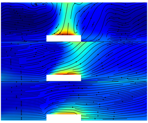
Pseudocolour plots of temperature (normalized by reference temperature) and velocity streamline in the  $z$–
 $x$ plane for different
 $M/w_{\ast ,r}$ but constant
 $w_{\ast ,u}/w_{\ast ,r}=3$ (low-resolution simulations as discussed in § 5.1). The white masked area contains both city blocks and streets (fluid space).

Using dimensional analysis and keeping the geometry-related parameters fixed for this study, two parameters are shown to govern the behaviour of circulations above cities: (1) the ratio of the convective velocity of the urban area to that of the rural area and (2) the ratio of the bulk/average inflow velocity to the convective velocity of the rural area. Depending on the relative magnitude of these two dimensionless parameters, city-scale circulations change from natural/pure convective-driven circulations, where the first ratio is the only important one, to advection-dominated circulations, where the second ratio solely controls the dynamics of circulations. An intermediate regime exists where both ratios are important, and ABL circulations are driven by both advection and convection processes (mixed convection). In addition, using the horizontal transects of the vertical velocity, we proposed a single a priori (based on external inputs) criterion to classify the different city-scale circulations (with different dimensionless parameters) into three regimes: bubble, transition and plume. The classification was then confirmed using blind  $k$-means clustering. While in this paper we only focused on the influence of urban/rural heat flux and bulk velocity of the flow, future studies are encouraged to investigate the effect of geometry-related parameters that were fixed in our study, such as city size and surface roughness.
The implications of this work for city ventilation, and how it is influenced by ABL-scale circulations, are myriad. We can already draw some conclusions regarding the effect of the flow regime on the thermal environment in the city, as illustrated in figure 15. The figure contrasts the temperature pseudocolour and velocity streamlines in the  $x$–
 $z$ plane for different circulation regimes. The cases are from the lower-resolution runs and for a constant
 $w_{\ast ,u}/w_{\ast ,r}=3$. One can note that for low
 $M/w_{\ast ,r}$ (bubble cases, minimum ventilation), the air above the city is hotter than at larger
 $M/w_{\ast ,r}$, and the heat generated in the city is lofted vertically above the city and recirculated back to the city. On the other hand, in the case of a plume regime (maximum ventilation), the heat is transported mostly downstream of the city (and leaves the domain) leading to a lower temperature in the city and a lower maximum temperature over the whole domain. The transitional regimes are associated with partially ventilated conditions. While these application-specific impacts will be more closely examined in follow-up studies, this paper lays the dimensional analysis and scaling grounds on which these subsequent studies can build.
Acknowledgements
This work is supported by the Army Research Office under contract W911NF-15-1-0003 (program manager J. Barzyk) and by the US National Science Foundation through ICER1664091 and CBET1444758 (Urban Water Innovation Network SRN). High-performance computing support from Cheyenne (doi:10.5065/D6RX99HX) provided by NCAR’s Computational and Information Systems Laboratory (NSF projects P36861020 and UPRI0007) is acknowledged.
Declaration of interests
The authors report no conflict of interest.
Appendix A. Sensitivity to street resolution
We tested the sensitivity of the results to the resolution of each street (the distance between blocks) for the advection regime (case 5) and the convection regime (case 7). Three cases were simulated with a different number of grid points for each street: 1 (as in low-resolution simulations of table 2), 3 (as in high-resolution simulations of table 1) and 5 (highest resolution). Note that the total area of heat emission equals the area of the city and is the same for all cases. Figure 16 shows maps of  $u$ for the advection-dominated regime with the three different street resolutions. It can be noted that, while
 $u$ for lower street resolutions is slightly smaller at the upstream edge of the city and behind the city (in the recirculation regime), overall the three cases show similar flow patterns. Flow blockage (pressure drag) is thus slightly stronger at lower resolutions. Similarly, figure 17 shows maps of
 $u$ for the convection-dominated regime with the three different street resolutions. We can see that circulations over the city in these cases are not very sensitive to the street resolutions. In both cases, the large-scale flow patterns that we are examining in this paper are not affected.
Pseudocolour plots of normalized (by average inflow)  $u$ for advection-dominated regime (case 5) with three different street resolutions. The white masked area contains both city blocks (solid space) and streets (fluid space).

Pseudocolour plots of normalized (by  $w_{\ast r}$)
 $w$ for convection-dominated regime (case 7) with three different street resolutions.

Appendix B. Precursor runs and rescaling of the inflow
The domain for the precursor runs has the same height ( $z$ direction) and width (
 $y$ direction) as the domain for the main runs (figure 2); however, the domain length for precursor runs is smaller than the main domain (3.5 km, with the same resolution as the main domain in all directions). Similar to the main domain, in inversion layer for the precursor domain covers the top 20 % of the domain height (and is maintained using the same approach as the main domain discussed in § 3.1). Therefore, the boundary layer height for the precursor runs is identical to the main domain and kept constant at 80 % of the domain height. The inflow variables (velocities and temperature) for the main domain runs were extracted from the end point (a
 $y$–
 $z$ slice) of the precursor domain runs. The inflow extraction is only started after the averaged TKE of the precursor domain reaches steady-state conditions.
For velocities, we can write the following relationships for the bulk velocity magnitudes for the rescaled precursor (with subscript  $p$), and the main precursor that is actually simulated (with subscript
 $m$) using MOST:
 $$\begin{eqnarray}\displaystyle & \displaystyle \frac{M_{p}}{u_{\ast ,p}}=\frac{1}{\unicode[STIX]{x1D705}}\left[\ln \left(\frac{z}{z_{0,r}}\right)+\unicode[STIX]{x1D6F9}_{M}\left(\frac{z}{L_{p}}\right)\right], & \displaystyle\end{eqnarray}$$
 $$\begin{eqnarray}\displaystyle & \displaystyle \frac{M_{m}}{u_{\ast ,m}}=\frac{1}{\unicode[STIX]{x1D705}}\left[\ln \left(\frac{z}{z_{0,r}}\right)+\unicode[STIX]{x1D6F9}_{M}\left(\frac{z}{L_{m}}\right)\right], & \displaystyle\end{eqnarray}$$
where  $z_{0,r}$ is the momentum roughness length of the rural area,
 $L$ the Obukhov length scale and
 $\unicode[STIX]{x1D6F9}_{M}$ the MOST stability function for momentum. If we approximate
 $\unicode[STIX]{x1D6F9}_{M}(z/L_{p})\approx \unicode[STIX]{x1D6F9}_{M}(z/L_{m})$, which is plausible given that the heat flux influencing
 $L_{p}$ and
 $L_{m}$ is the same although the friction velocities are different, then
 $M_{p}$ can be calculated by rescaling the average of the generated main inflow in the main precursor simulation to get the desired inflow as follows:
 $$\begin{eqnarray}M_{p}=\frac{u_{\ast ,p}}{u_{\ast ,m}}M_{m}.\end{eqnarray}$$
The same scaling is then used to generate the whole inflow planes for  $u$,
 $v$ and
 $w$ as functions of
 $y$,
 $z$ and
 $t$. Using (B 3), we are able to use one generated inflow velocity for each of the rural heat fluxes to produce a range of precursor inflows with different bulk-averaged velocities.
For temperature, we can also invoke MOST to write the temperature profile for precursor simulations and main runs as follows:
 $$\begin{eqnarray}\displaystyle & \displaystyle \unicode[STIX]{x1D703}_{s}^{inflow}-\unicode[STIX]{x1D703}_{m}^{inflow}=\frac{1}{\unicode[STIX]{x1D705}}\frac{(\overline{\unicode[STIX]{x1D703}^{\prime }w^{\prime }})_{r}}{u_{\ast ,m}}\left[\ln \left(\frac{z}{z_{0,h}^{r}}\right)+\unicode[STIX]{x1D6F9}_{\unicode[STIX]{x1D703}}\left(\frac{z}{L_{p}}\right)\right], & \displaystyle\end{eqnarray}$$
 $$\begin{eqnarray}\displaystyle & \displaystyle \unicode[STIX]{x1D703}_{s}^{inflow}-\unicode[STIX]{x1D703}_{p}^{inflow}=\frac{1}{\unicode[STIX]{x1D705}}\frac{(\overline{\unicode[STIX]{x1D703}^{\prime }w^{\prime }})_{r}}{u_{\ast ,p}}\left[\ln \left(\frac{z}{z_{0,h}^{r}}\right)+\unicode[STIX]{x1D6F9}_{\unicode[STIX]{x1D703}}\left(\frac{z}{L_{p}}\right)\right], & \displaystyle\end{eqnarray}$$
where  $z_{0,h}^{r}=0.1z_{0,m}^{r}$ is the heat roughness length of the rural area and
 $\unicode[STIX]{x1D703}_{s}^{inflow}$ is the surface temperature for the inflow that is assumed to be equal for both precursor and main simulations. Assuming
 $(\unicode[STIX]{x1D6F9}_{\unicode[STIX]{x1D703}}(z/L_{p}))/M_{p}\approx (\unicode[STIX]{x1D6F9}_{\unicode[STIX]{x1D703}}(z/L_{m}))/M_{m}$ and subtracting (B 5) from (B 4), we obtain the following rescaling relation between the temperatures of the precursor and main simulations:
 $$\begin{eqnarray}\unicode[STIX]{x1D703}_{p}^{inflow}=\unicode[STIX]{x1D703}_{m}^{inflow}+\frac{1}{\unicode[STIX]{x1D705}}(\overline{\unicode[STIX]{x1D703}^{\prime }w^{\prime }})_{r}\ln \left(\frac{z}{z_{0,h}^{r}}\right)\left(\frac{1}{M_{m}}-\frac{1}{M_{p}}\right).\end{eqnarray}$$
We reiterate that this rescaling need not be exact since (i) the inflow is allowed to evolve over a distance of approximately five times the boundary layer depth  $(1800~\text{m}/333~\text{m})$ inside the main domain to further adjust to the upstream rural surface before it meets the city and (ii) regardless of the rescaling results, the
 $M$ used in the analyses is the one actually attained and computed just upstream of the city in the main domain.
Appendix C. Sensitivity to domain size
Figure 18 shows the maps of the cross-stream velocity  $v$ in the
 $z$–
 $y$ plane for three different values of
 $L_{y}/L_{c}=3.8$, 5 and 5.6 (they correspond to
 $L_{y}=3330$, 4500 and 5000 m). All three simulations are conducted for the case without inflow (case 7 in table 1). This case corresponds to the largest circulations around the city; therefore, we can use it to investigate the minimum domain size needed to prevent circulations from strongly interacting with each other across the periodic boundaries. One can observe that in the case of
 $L_{y}/L_{c}=3.8$ (
 $L_{y}=3330~\text{m}$), the circulations clearly interact with the left and right boundaries, and this leads to a rightward shift in the position of the circulations above the city (this could have as well been a deflection to the left). On the other hand, for the other two cases (
 $L_{y}/L_{c}=5$ and 5.6), the horizontal extent of the circulations on either side of the city is roughly equal to three times the city size; hence, the size of the domain in these cases is large enough to prevent the city circulations from directly interacting and does not affect the circulation scale. Figure 18 also shows that indirect interactions through intermediate circulations are weak since these intermediate structures are less energetic. For all of the simulations in table 1, we chose the intermediate domain size where
 $L_{y}/L_{c}=5$ (
 $L_{y}=4500~\text{m}$).
Pseudocolour maps of normalized (by  $w_{\ast r}$)
 $v$ in the
 $z$–
 $y$ plane for convection-dominated regime (case 7) with three different
 $L_{y}/L_{c}$: 3.8 (a), 5 (b) and 5.6 (c).

Appendix D. Turbulent kinetic energy
Figure 19 displays the horizontal profile of normalized (resolved) TKE for different regimes (transitional, plume and bubble). Similar to the mean velocities, the higher-order statistics also follow the scaling similarity derived in this paper. For the transitional regime, cases 1 and 2 show similar TKE profiles that are distinct from those in cases 3 and 4. Similar conclusions can be drawn for plume (cases 5 and 6) and bubble (cases 7 and 8) regimes, not shown here.
Horizontal profiles of normalized (by  $w_{\ast r}^{2}$) TKE for transitional (a), plume (b) and bubble (c) regimes.



