1 Introduction
Laminar boundary layers over swept aeroplane wings are commonly approximated by the Falkner–Skan–Cooke (FSC) similarity solutions (Falkner & Skan Reference Falkner and Skan1931; Cooke Reference Cooke1950). For such flows, the dominating features in low-disturbance environments, e.g. free flight, are the spatially developing stationary cross-flow (CF) vortices. It is generally established that the stationary CF vortices are mainly initiated by surface roughness, while free-stream turbulence promotes travelling CF waves (see Saric, Reed & White (Reference Saric, Reed and White2003) and the references therein). The CF modes are linked with attachment-line modes (Mack, Schmid & Sesterhenn Reference Mack, Schmid and Sesterhenn2008) and exhibit convective instability (Wassermann & Kloker Reference Wassermann and Kloker2002), meaning that they act as noise amplifiers. They typically break down to turbulence by secondary instabilities (Högberg & Henningson Reference Högberg and Henningson1998; Malik et al. Reference Malik, Li, Choudhari and Chang1999; Wassermann & Kloker Reference Wassermann and Kloker2002).
In the case of a roughness element inside the boundary layer, the local flow conditions around the roughness can be characterised by a roughness Reynolds number
 $Re_{k}$
, which in two-dimensional boundary layers is defined by the roughness height and the local undisturbed streamwise velocity at the roughness height. By increasing
 $Re_{k}$
in a two-dimensional boundary layer beyond a certain limit,
 $Re_{k,t}$
, the transition location has been observed to move upstream to the trailing edge of the roughness (von Doenhoff & Braslow Reference von Doenhoff, Braslow and Lachmann1961). Due to its importance for the development of laminar wings, the determination of
 $Re_{k,t}$
has been the subject of several global stability analyses (Loiseau et al.
Reference Loiseau, Robinet, Cherubini and Leriche2014; Citro et al.
Reference Citro, Giannetti, Luchini and Auteri2015; Kurz & Kloker Reference Kurz and Kloker2016). For roughness elements in a Blasius boundary layer, the above-mentioned flow tripping was found to correspond to the onset of a global flow instability. However, for swept-wing boundary layers, the situation is more complex, as recently demonstrated by Kurz & Kloker (Reference Kurz and Kloker2016). These authors carried out a comprehensive direct numerical simulation (DNS) study accompanied by a global stability analysis and noted a sensitivity of the unstable eigenvalue spectra with respect to numerical parameters and domain size. However, the origin of these issues was not investigated in detail in their work.
Domain-dependent spectra for unstable flows are scarcely reported and discussed in the literature. In many cases, the onset of global instability is associated with one pair of complex conjugate eigenvalues that destabilises through a supercritical Hopf bifurcation as some bifurcation parameter is varied (Loiseau et al. Reference Loiseau, Robinet, Cherubini and Leriche2014; Citro et al. Reference Citro, Giannetti, Luchini and Auteri2015; Peplinski, Schlatter & Henningson Reference Peplinski, Schlatter and Henningson2015). Such intrinsic oscillations can sometimes be insensitive to numerical details, and be independent of domain size if the overlap between the corresponding direct and adjoint eigenfunctions is included in the domain (Giannetti & Luchini Reference Giannetti and Luchini2007). In contrast, stable eigenvalues along an eigenvalue branch can in many situations be very sensitive with respect to numerical parameters, e.g. eigenvalue shifts or domain sizes (Ehrenstein & Gallaire Reference Ehrenstein and Gallaire2005; Alizard & Robinet Reference Alizard and Robinet2007; Garnaud et al. Reference Garnaud, Lesshafft, Schmid and Huerre2013; Cerqueira & Sipp Reference Cerqueira and Sipp2014). For such flows, a resolvent or impulse-response analysis may be more appropriate.
In the present work, the global stability of a FSC boundary layer with a cylindrical surface roughness is considered. In particular, the sensitivity of the eigenvalue spectra to numerical parameters and domain dependency is addressed and an explanation of this behaviour is provided.
2 Flow configuration and numerical approach
2.1 Baseflow
Here, a FSC boundary layer characterised by a constant free-stream velocity in the spanwise direction and an accelerating velocity in the streamwise direction is considered,
 $$\begin{eqnarray}\displaystyle & U_{\infty }^{\ast }(x^{\ast })=U_{0}^{\ast }(x^{\ast }/x_{0}^{\ast })^{m}, & \displaystyle\end{eqnarray}$$
 $$\begin{eqnarray}\displaystyle & W_{\infty }^{\ast }=W_{0}^{\ast }. & \displaystyle\end{eqnarray}$$
A superscript asterisk denotes dimensional quantities, subscript
 $\infty$
the flow outside the boundary layer and subscript 0 quantities at the inflow. The acceleration of the flow causes the inviscid streamlines to be curved. In the inviscid region a balance between centrifugal and pressure forces exists, but inside the boundary layer, where the streamwise velocity decreases, a force imbalance arises that generates a CF component perpendicular to the inviscid streamline (Saric et al.
Reference Saric, Reed and White2003). This CF component is inflectionally unstable (Gregory, Stuart & Walker Reference Gregory, Stuart and Walker1955). The FSC velocity profiles are derived in appendix A. See also Falkner & Skan (Reference Falkner and Skan1931) and Cooke (Reference Cooke1950) for further details.
All quantities are non-dimensionalised using the displacement thickness
 $\unicode[STIX]{x1D6FF}_{0}^{\ast }$
and the free-stream streamwise velocity
 $U_{0}^{\ast }$
. The numerical parameter values used in this study are similar to those used by Högberg & Henningson (Reference Högberg and Henningson1998). The distance from the leading edge to the beginning of the domain is
 $x_{0}=354.0$
, the spanwise free-stream velocity is
 $W_{0}=1.442$
, the acceleration parameter is
 $m=0.34207$
and the inflow Reynolds number based on the streamwise velocity and displacement thickness is
 $Re_{\unicode[STIX]{x1D6FF}_{0}^{\ast }}=337.9$
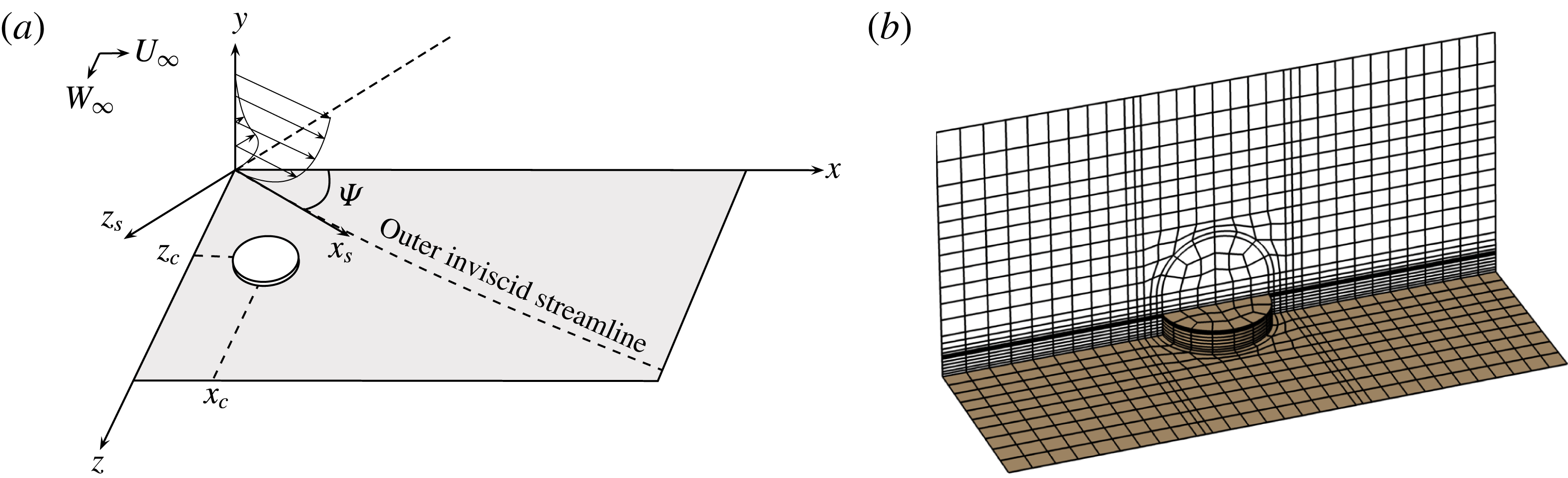
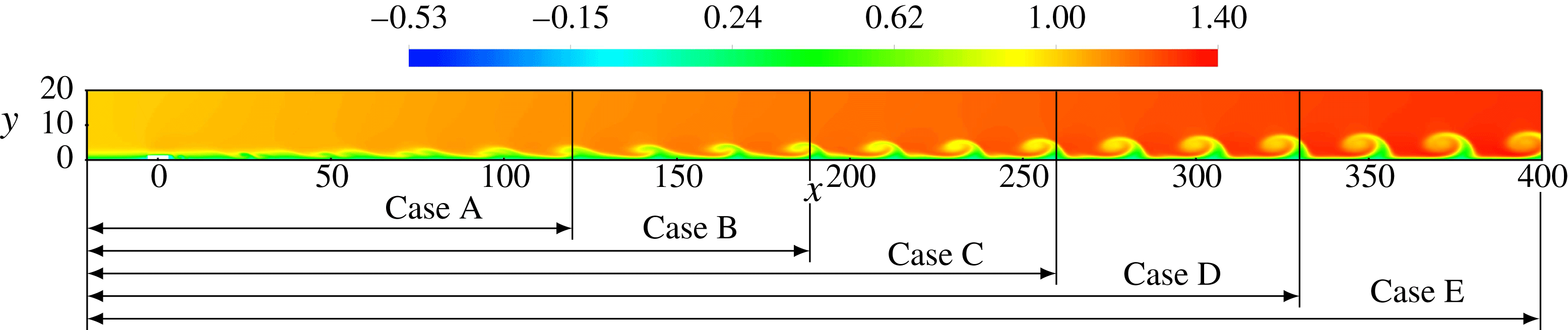
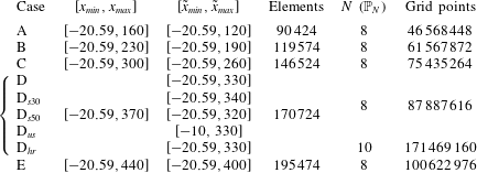
. A sketch illustrating the set-up is given in figure 1(a). The computational domain consists of a rectangular box with a spanwise width of 25.14 (chosen to match the wavelength of the most unstable stationary CF mode; see Högberg & Henningson Reference Högberg and Henningson1998), a height of 20.0 and various streamwise lengths according to table 1 (see also figure 2).
Overview of the flow case and set-up. The sketch in (a) illustrates the coordinate system and the velocity profiles aligned and perpendicular to the inviscid streamline. The surface roughness and the mesh structure is visualised in (b).

Visualisation of the baseflow structures for the various cases listed in table 1 (streamwise component shown). The roughness is centred at the origin.

Cases considered;
 $\unicode[STIX]{x1D6FA}=[x_{min},x_{max}]\times [0,20]\times [-12.57,12.57]$
denotes the computational domain for cases A–E and
 $\tilde{\unicode[STIX]{x1D6FA}}=[\tilde{x}_{min},\tilde{x}_{max}]\times [0,20]\times [-12.57,12.57]$
the corresponding region outside of the support of the sponge function.

2.2 Numerical method
The flow is governed by the time-dependent incompressible Navier–Stokes equations subject to constant fluid properties:
 $$\begin{eqnarray}\displaystyle \frac{\unicode[STIX]{x2202}\boldsymbol{U}}{\unicode[STIX]{x2202}t}+\boldsymbol{U}\boldsymbol{\cdot }\unicode[STIX]{x1D735}\boldsymbol{U} & = & \displaystyle -\unicode[STIX]{x1D735}P+\frac{1}{Re_{\unicode[STIX]{x1D6FF}_{0}^{\ast }}}\unicode[STIX]{x1D6FB}^{2}\boldsymbol{U}+\boldsymbol{F}\quad \text{in }\unicode[STIX]{x1D6FA},\end{eqnarray}$$
 $$\begin{eqnarray}\displaystyle \unicode[STIX]{x1D735}\boldsymbol{\cdot }\boldsymbol{U} & = & \displaystyle 0\quad \text{in }\unicode[STIX]{x1D6FA},\end{eqnarray}$$
 $\boldsymbol{U}=(U,V,W)^{\text{T}}$
denotes the velocity components in
 $x$
-,
 $y$
- and
 $z$
-directions and
 $\unicode[STIX]{x1D6FA}$
is the domain, defined in the caption of table 1. The term
 $\boldsymbol{F}$
is a volume force, which in the nonlinear DNS consists of a sponge force defined as
 $\unicode[STIX]{x1D706}(x)(\boldsymbol{U}_{FSC}-\boldsymbol{U})$
, where the subscript FSC denotes the FSC profiles and
 $\unicode[STIX]{x1D706}(x)$
is given by (2.8). In the baseflow computations,
 $\boldsymbol{F}$
consists of the force due to selective frequency damping (SFD, Åkervik et al.
Reference Åkervik, Brandt, Henningson, Hœpffner, Marxen and Schlatter2006), as discussed below. Equation (2.3) is integrated in time using the high-order DNS code Nek5000 (Fischer, Lottes & Kerkemeier Reference Fischer, Lottes and Kerkemeier2008), which is based upon the spectral-element method (SEM). The velocity and pressure fields are discretised using a
 $\mathbb{P}_{N}$
–
 $\mathbb{P}_{N-2}$
formulation, where
 $N$
th-degree Lagrange interpolation polynomials on the Gauss–Lobatto–Legendre quadrature points and
 $(N-2)$
th-degree Lagrange interpolation polynomials on the Gauss–Legendre quadrature points are chosen as basis functions for the velocity and the pressure, respectively (see Deville, Fischer & Mund (Reference Deville, Fischer and Mund2002) for further details).
As inflow conditions, the FSC velocity profiles are prescribed. In the spanwise direction periodic conditions are assigned (only one flow period is simulated), and at the wall an ordinary no-slip condition is used. The outflow boundary conditions read
 $\unicode[STIX]{x2202}_{x}V=0$
,
 $\unicode[STIX]{x2202}_{x}W=0$
and
 $Re_{\unicode[STIX]{x1D6FF}_{0}^{\ast }}^{-1}\unicode[STIX]{x2202}_{x}U-P=-P_{a}$
(where
 $P_{a}=-Re_{\unicode[STIX]{x1D6FF}_{0}^{\ast }}^{-1}\unicode[STIX]{x2202}_{x}U_{FSC}$
represents an ambient pressure). Along the free-stream boundary
 $U=U_{\infty }(x)$
,
 $W=W_{\infty }$
(see appendix A) and
 $Re_{\unicode[STIX]{x1D6FF}_{0}^{\ast }}^{-1}\unicode[STIX]{x2202}_{y}V-P=-P_{b}$
(where
 $P_{b}=\tilde{P}-Re_{\unicode[STIX]{x1D6FF}_{0}^{\ast }}^{-1}\unicode[STIX]{x2202}_{y}V_{FSC}$
, with
 $\tilde{P}$
obtained from inserting the FSC velocities into the Bernoulli equation).
In order to obtain a baseflow
 $\boldsymbol{U}$
, SFD (Åkervik et al.
Reference Åkervik, Brandt, Henningson, Hœpffner, Marxen and Schlatter2006) is used. This implies applying a volume force
 $\boldsymbol{F}=-\unicode[STIX]{x1D712}(\boldsymbol{U}-\bar{\boldsymbol{U}})$
to (2.3a
) that forces the flow towards a temporally low-pass-filtered target solution
 $\bar{\boldsymbol{U}}$
. As (2.3) is integrated in time and the solution approaches the target, the magnitude of the force decreases, thus yielding a steady solution of the unforced Navier–Stokes equations upon convergence. The norm of the difference between the instantaneous and the filtered velocity is used as a measure of convergence, and the equations are integrated until this quantity is below
 $10^{-8}$
. SFD requires two design parameters to be calibrated – a filter gain
 $\unicode[STIX]{x1D712}$
related to the temporal growth rate of the instability and a filter width
 $\unicode[STIX]{x1D6E5}$
related to its frequency. These are chosen to be
 $\unicode[STIX]{x1D712}=0.4$
and
 $\unicode[STIX]{x1D6E5}=8/\unicode[STIX]{x03C0}$
.
The streamwise extents of the different cases listed in table 1 are illustrated in figure 2. As seen, extending the domain in the streamwise direction implies that stronger CF vortices will be included in the computational domain. Stability analysis of such large domains necessarily requires the use of matrix-free methods. To this end, time-stepping techniques as described by e.g. Bagheri et al. (Reference Bagheri, Åkervik, Brandt and Henningson2009) are employed. The dynamics of a small perturbation
 $\boldsymbol{u}$
about the baseflow,
 $\boldsymbol{U}$
, is governed by the linearised Navier–Stokes equations
 $$\begin{eqnarray}\displaystyle \frac{\unicode[STIX]{x2202}\boldsymbol{u}}{\unicode[STIX]{x2202}t}+\boldsymbol{u}\boldsymbol{\cdot }\unicode[STIX]{x1D735}\boldsymbol{U}+\boldsymbol{U}\boldsymbol{\cdot }\unicode[STIX]{x1D735}\boldsymbol{u} & = & \displaystyle -\unicode[STIX]{x1D735}p+\frac{1}{Re_{\unicode[STIX]{x1D6FF}_{0}^{\ast }}}\unicode[STIX]{x1D6FB}^{2}\boldsymbol{u}+\boldsymbol{f}\quad \text{in }\unicode[STIX]{x1D6FA},\end{eqnarray}$$
 $$\begin{eqnarray}\displaystyle \unicode[STIX]{x1D735}\boldsymbol{\cdot }\boldsymbol{u} & = & \displaystyle 0\quad \text{in }\unicode[STIX]{x1D6FA},\end{eqnarray}$$
 $\boldsymbol{f}$
represents a volume force. This can conveniently be expressed in operator form as
 $\unicode[STIX]{x2202}\boldsymbol{u}/\unicode[STIX]{x2202}t={\mathcal{L}}_{\boldsymbol{U}}\boldsymbol{u}$
, treating pressure as a dependent variable. Upon introducing a global mode ansatz
 $\boldsymbol{u}(\boldsymbol{x},t)=\hat{\boldsymbol{u}}(\boldsymbol{x})\text{e}^{-\text{i}\unicode[STIX]{x1D714}t}+\text{c.c.}$
and discretising (2.4), one arrives at the generalised eigenvalue problem
 $$\begin{eqnarray}\unicode[STIX]{x1D647}\hat{\boldsymbol{u}}=-\text{i}\unicode[STIX]{x1D714}\unicode[STIX]{x1D648}\hat{\boldsymbol{u}},\end{eqnarray}$$
where
 $\unicode[STIX]{x1D647}$
is the discrete linearised Navier–Stokes operator
 ${\mathcal{L}}_{\boldsymbol{U}}$
,
 $\unicode[STIX]{x1D648}$
denotes the mass matrix and
 $(\hat{\boldsymbol{u}},-\text{i}\unicode[STIX]{x1D714})$
is a complex eigenpair. The eigenvalue problem (2.5) is solved by integrating the initial condition
 $\boldsymbol{u}(\boldsymbol{x},0)$
(random noise) in time with a time stepper (Nek5000), below denoted by
 $\unicode[STIX]{x1D63D}(\unicode[STIX]{x0394}t)$
. By repeated application of
 $\unicode[STIX]{x1D63D}(\unicode[STIX]{x0394}t)\approx \exp (\unicode[STIX]{x1D63C}\unicode[STIX]{x0394}t)$
, where
 $\unicode[STIX]{x1D63C}=\unicode[STIX]{x1D648}^{-1}\unicode[STIX]{x1D647}$
, solution fields separated in time by
 $\unicode[STIX]{x0394}t$
are assembled to span a low-dimensional Krylov space
 $$\begin{eqnarray}\displaystyle {\mathcal{K}}_{n} & = & \displaystyle \text{span}\{\boldsymbol{u}(\boldsymbol{x},0),\boldsymbol{u}(\boldsymbol{x},\unicode[STIX]{x0394}t),\boldsymbol{u}(\boldsymbol{x},2\unicode[STIX]{x0394}t),\ldots ,\boldsymbol{u}(\boldsymbol{x},(n-1)\unicode[STIX]{x0394}t)\}\nonumber\\ \displaystyle & = & \displaystyle \text{span}\{\boldsymbol{u}(\boldsymbol{x},0),\unicode[STIX]{x1D63D}(\unicode[STIX]{x0394}t)\boldsymbol{u}(\boldsymbol{x},0),\unicode[STIX]{x1D63D}^{2}(\unicode[STIX]{x0394}t)\boldsymbol{u}(\boldsymbol{x},0),\ldots ,\unicode[STIX]{x1D63D}^{n-1}(\unicode[STIX]{x0394}t)\boldsymbol{u}(\boldsymbol{x},0)\}.\end{eqnarray}$$
As a means of determining the dominant eigenpairs of (2.5), the Krylov vectors spanning
 ${\mathcal{K}}_{n}$
are factorised to satisfy an Arnoldi relation,
 $$\begin{eqnarray}\unicode[STIX]{x1D63D}(\unicode[STIX]{x0394}t)\unicode[STIX]{x1D651}_{n}=\unicode[STIX]{x1D651}_{n}\unicode[STIX]{x1D643}_{n}+\boldsymbol{r}_{n}\boldsymbol{e}_{n}^{\text{T}},\end{eqnarray}$$
such that the eigenpairs of
 $\unicode[STIX]{x1D63C}$
can be approximated from the eigenpairs of the
 $n\times n$
upper Hessenberg matrix
 $\unicode[STIX]{x1D643}_{n}$
, which represents the projection of
 $\unicode[STIX]{x1D63D}(\unicode[STIX]{x0394}t)$
onto
 ${\mathcal{K}}_{n}$
spanned by the columns of
 $\unicode[STIX]{x1D651}_{n}$
(
 $\boldsymbol{r}_{n}\boldsymbol{e}_{n}^{\text{T}}$
is the residual of the factorisation). See Bagheri et al. (Reference Bagheri, Åkervik, Brandt and Henningson2009) for further details.
The implementation (Peplinski et al.
Reference Peplinski, Schlatter, Fischer, Henningson, Azaïez, El Fekih and Hesthaven2014) is based on the implicitly restarted Arnoldi method (IRAM) from the ARPACK library (Lehoucq, Sorensen & Yang Reference Lehoucq, Sorensen and Yang1997). For these computations periodic boundary conditions are imposed in the spanwise direction, and in all other directions homogeneous Dirichlet conditions are prescribed. A sponge region is added at the downstream end of the domain in order to dampen reflections and make the flow satisfy the boundary conditions. This is defined as
 $\boldsymbol{f}=-\unicode[STIX]{x1D706}(x)\boldsymbol{u}$
, where
 $$\begin{eqnarray}\displaystyle \unicode[STIX]{x1D706}(x) & = & \displaystyle \unicode[STIX]{x1D706}_{max}S\left(\frac{x-x_{start}}{\unicode[STIX]{x1D6E5}_{rise}}\right),\end{eqnarray}$$
 $$\begin{eqnarray}\displaystyle S(x) & = & \displaystyle \left\{\begin{array}{@{}ll@{}}0,\quad & x\leqslant 0,\\ \text{}[1+\exp (1/(x-1)+1/x)]^{-1},\quad & 0<x<1,\\ 1,\quad & x\geqslant 1\end{array}\right.\end{eqnarray}$$
 $\unicode[STIX]{x1D706}_{max}=1$
,
 $\unicode[STIX]{x1D6E5}_{rise}=25$
and
 $x_{start}$
is chosen to give a sponge length according to table 1. In the stability computations presented in this work, 100 dominant eigenmodes were determined using a tolerance of
 $10^{-6}$
for IRAM (see Lehoucq et al. (Reference Lehoucq, Sorensen and Yang1997) for information on the convergence criterion).
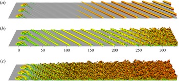
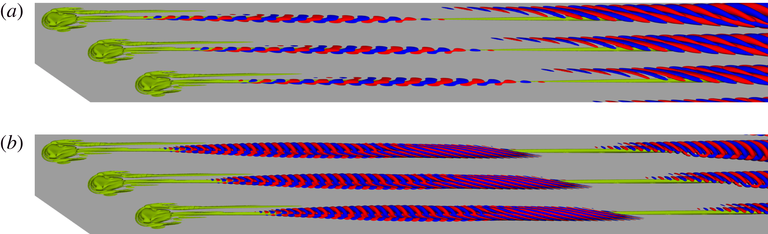
Flow visualisation for different
 $k$
(three spanwise periods shown): (a)
 $k=0.9$
,
 $Re_{k}=233.96$
; (b)
 $k=1.3$
,
 $Re_{k}=458.01$
; (c)
 $k=1.7$
,
 $Re_{k}=728.63$
. Contours of streamwise velocity are plotted in light grey and contours of negative
 $\unicode[STIX]{x1D706}_{2}$
(Jeong & Hussain Reference Jeong and Hussain1995) are coloured by streamwise velocity.

2.3 Surface roughness
A cylindrical surface roughness with diameter
 $d=6.0$
visualised in figure 1(b) is introduced into the domain with its centre located at the origin of the coordinate system,
 $x_{c}=z_{c}=0$
(i.e. 20.59 downstream of the inflow). Results from initial nonlinear DNS of roughness elements with heights
 $k=\{0.9,1.3,1.7\}$
corresponding to
 $Re_{k}=\{233.96,458.01,728.63\}$
(based on the wall-parallel velocity
 $\sqrt{U_{FSC}^{2}+W_{FSC}^{2}}$
) in the domain
 $\unicode[STIX]{x1D6FA}^{D}$
are shown in figure 3. The flow induced by the lowest roughness with
 $k=0.9$
(figure 3
a) is dominated by large corotating CF vortices that emanate from the vortex structure in the near-field roughness wake. After an initial transient phase the flow becomes stationary. Increasing the roughness height to
 $k=1.3$
(figure 3
b) gives stronger CF vortices that transition to turbulence through a mechanism resembling a secondary instability (cf. Wassermann & Kloker Reference Wassermann and Kloker2002). From figure 3(b) unsteady finger-like vortices are seen to appear around
 $x\approx 150$
, and a probe inside the boundary layer (marked with a white bullet in figure 3
b) measures a band of frequencies around 1.0 (not shown), which can be compared with 0.957 reported by Högberg & Henningson (Reference Högberg and Henningson1998). This suggests that the CF vortices in this case reach sufficient magnitude to be destabilised through secondary instabilities. Further increase of the roughness height to
 $k=1.7$
(figure 3
c) gives an immediate breakdown to turbulence behind the roughness reminiscent of those observed in two-dimensional boundary layers (Loiseau et al.
Reference Loiseau, Robinet, Cherubini and Leriche2014; Citro et al.
Reference Citro, Giannetti, Luchini and Auteri2015). The flow fields plotted in figure 3 were extracted after transients had decayed or been advected out of the domain. Based on this initial DNS study, one can tentatively say that for this set-up, the critical roughness height, i.e. the height that first causes flow instability in the domain, lies between 0.9 and 1.3. In light of this, the roughness element with
 $k=1.3$
is selected for further analysis.
Overview of the baseflow details: (a) the vortex structures around the roughness visualised with the
 $\unicode[STIX]{x1D706}_{2}$
-criterion (Jeong & Hussain Reference Jeong and Hussain1995) (green); (b) the development of these vortex structures in space together with
 $U-U_{FSC}$
(colour) and
 $U$
(black contour) in
 $yz$
-slices at the indicated
 $x$
-positions.

Eigenvalue sensitivity with respect to solver tolerance, resolution and sponge length. (a) Spectra for the case D with tolerance
 $10^{-10}$
(○) together with its
 $\unicode[STIX]{x1D700}$
-pseudospectrum (logarithmically spaced coloured contours of
 $\unicode[STIX]{x1D700}$
), case D with tolerance
 $10^{-8}$
(
 $+$
) and case D
 $_{hr}$
(✳). (b) Spectra for case D (○), D
 $_{s30}$
(♢) and D
 $_{s50}$
(
 $+$
).

2.4 Vortex system
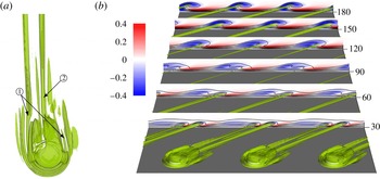
An account of the vortex structures surrounding a smooth roughness element positioned on a wing was recently given by Kurz & Kloker (Reference Kurz and Kloker2016). For the cylindrical roughness on a swept plate, a similar vortex system may be identified, and is presented for the intermediate roughness element (
 $k=1.3$
) in figure 4. From the vortex visualisation in figure 4(a), a set of tightly wrapped horseshoe vortices are identified that winds around the frontal rim of the roughness. The strongest of these vortices is labelled ‘1’ and marked in figure 4(a). Another pair of vortices emanate from the reversed flow region behind the roughness and the flow going over the roughness. The most prominent of these is labelled ‘2’.
This vortex system can be compared with that developing behind a cylindrical roughness element in a Blasius boundary layer, where the wake is symmetric and consists of a central rapidly decaying low-speed streak and an outer pair of high- and low-speed streaks (Loiseau et al.
Reference Loiseau, Robinet, Cherubini and Leriche2014). In contrast, the roughness wake in the FSC boundary layer is seen to be completely asymmetric, even in the vicinity of the roughness. As shown in figure 4(b), the right leg of vortex ‘1’ (on the leeward side of the roughness) decays quickly, whereas the left leg (on the windward side) extends over a considerable downstream distance alongside vortex ‘2’, which together induces two high- and low-speed streaks. Eventually, the left leg of vortex ‘1’ also decays and merges with vortex ‘2’ (between
 $60<x<90$
). This leads to an annihilation of the leftmost high-speed streak such that at
 $x\approx 120$
a single vortex prevails together with a high- and low-speed streak. This coalesced vortex strengthens further downstream and develops into the CF vortex, as opposed to the vortical structures induced in a Blasius boundary layer, which eventually decay. As shown in the next section, this difference turns out to have a tremendous effect on the stability characteristics of the flow.
3 Global stability and sensitivity analysis
Following the temporal stability framework with the ansatz function introduced in § 2.2, the eigenvalues are
 $(-\text{i}\unicode[STIX]{x1D714})$
. By adopting the definition of global instability common in the literature, a flow will be termed globally stable if the real parts of all eigenvalues are negative, and conversely globally unstable if at least one eigenvalue has a positive real part. The term critical refers to a configuration that is marginally stable, i.e. where the least stable eigenvalue has a vanishing real part (is close to zero).
3.1 Eigenvalue sensitivity
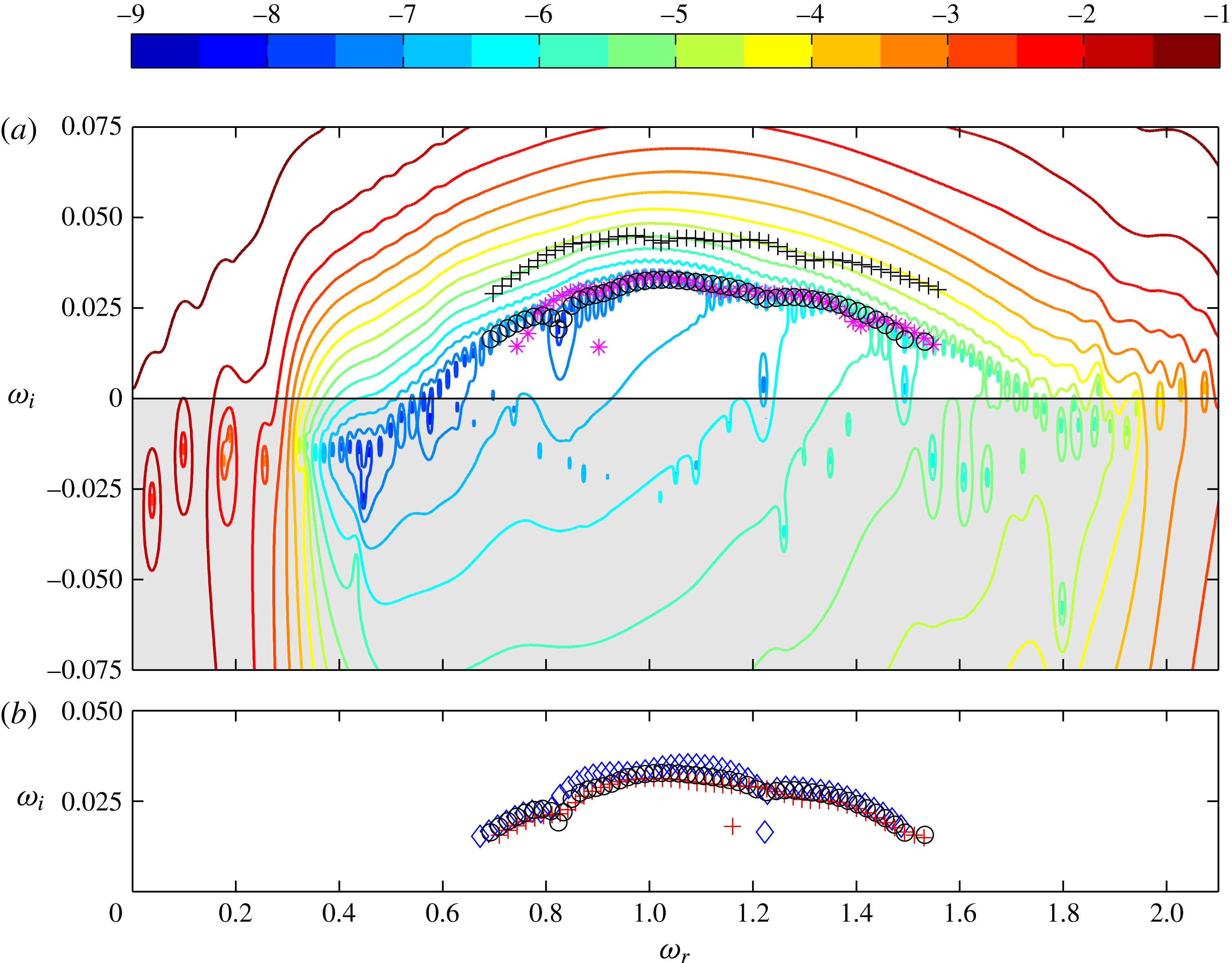
The eigenvalues from the stability analysis of case D are shown in figure 5(a). Clearly, all the reported eigenvalues are unstable, which shows that the transition observed in figure 3(b) actually corresponds to a global flow instability. For this case two polynomial orders for the perturbation, two solver tolerances and different sponge lengths are investigated (see table 1).
The sensitivity of the spectrum to resolution is investigated by increasing the polynomial order from
 $N=8$
to
 $N=10$
(case D
 $_{hr}$
). This amounts to a near doubling of the number of grid points. As seen in figure 5(a), the spectra are slightly different but overlapping, which shows that the flow is sensitive to numerical details but sufficiently resolved in space.
The sensitivity of the spectrum to the iterative solver tolerance is often overlooked in this type of study. The convergence of the velocity and the pressure solver (see Deville et al.
Reference Deville, Fischer and Mund2002) are monitored by tracking the norm of the solution residual and the divergence of the velocity, respectively. Throughout all the computations, the solver tolerances are set to
 $10^{-10}$
(unless otherwise stated in the text). However, as shown in figure 5(a), changing these tolerances from
 $10^{-10}$
to
 $10^{-8}$
almost doubles the computed growth rates. Sensitivity of the spectra to numerical parameters has been reported for strongly damped eigenmodes by e.g. Cerqueira & Sipp (Reference Cerqueira and Sipp2014), who concluded that it was impossible to find a unique set of eigenvalues that were intrinsic to their flow. One can view a change in the solver tolerance as effectively imposing a small perturbation on the governing matrix for the flow. As such, the reported eigenvalues should be interpreted as
 $\unicode[STIX]{x1D700}$
-pseudoeigenvalues, defined as the eigenvalues of a perturbed matrix, i.e. the eigenvalues of
 $(\unicode[STIX]{x1D63C}+\unicode[STIX]{x1D640})$
where
 $\unicode[STIX]{x1D640}$
is a perturbation with
 $\Vert \unicode[STIX]{x1D640}\Vert \leqslant \unicode[STIX]{x1D700}$
(Trefethen Reference Trefethen1992; Schmid & Henningson Reference Schmid and Henningson2001). A consequence of this view is, for instance, that two similar calculations initiated with slightly different random noise never can be expected to give exactly the same eigenvalues. This is because any number
 $\unicode[STIX]{x1D70E}$
sampled from a pseudospectral contour line for which the resolvent norm
 $\Vert (\unicode[STIX]{x1D70E}\unicode[STIX]{x1D644}-\unicode[STIX]{x1D63C})^{-1}\Vert$
attains a sufficiently large value may be interpreted as an eigenvalue by the solver. Inspection of the pseudospectral contours suggests that further increases in solver tolerance will not stabilise the eigenvalues in this case, since these curves are both nested and bounded from below. Moreover, determining very sensitive eigenvalues like those plotted in figure 5(a) to any greater precision is of limited value. The
 $\unicode[STIX]{x1D700}$
-pseudospectrum in figure 5(a) is computed by evaluating the resolvent norm for the logarithm of the Hessenberg matrix from the Arnoldi factorisation (2.7) of case D,
 $\log (\unicode[STIX]{x1D643}_{n})/\unicode[STIX]{x0394}t$
(Toh & Trefethen Reference Toh and Trefethen1996). Since
 $\unicode[STIX]{x1D643}_{n}$
is of modest size, this can be done by determining the smallest singular value of
 $[\unicode[STIX]{x1D70E}\unicode[STIX]{x1D644}-\log (\unicode[STIX]{x1D643}_{n})/\unicode[STIX]{x0394}t]$
, where
 $\unicode[STIX]{x1D70E}$
is a complex number (Trefethen Reference Trefethen1992).
In line with the above discussion, it is instructive to also consider the sensitivity of the spectrum with respect to the sponge length. This is done by varying the sponge length by
 $\pm 10$
units for case D (cases D
 $_{s30}$
and D
 $_{s50}$
). As seen in figure 5(b), this parameter has a negligible effect on the stability, which suggests that the treatment of the outflow boundary is satisfactory.
3.2 Domain dependency
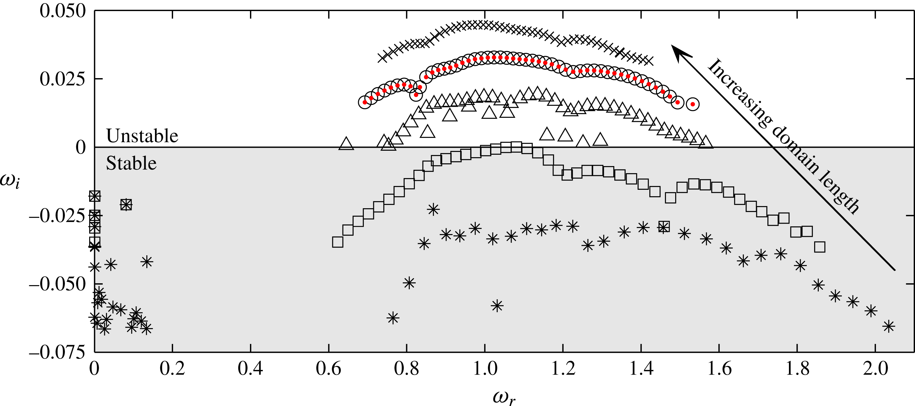
For the boundary layer studied here, the growth of CF vortices is promoted in the entire domain as visualised in figure 2. Figure 6 shows the eigenvalue spectrum for the cases A–E. In case B, the flow is found to be marginally stable, which can be compared to the location at which unsteady vortices appear in figure 3(b). Notably, the flow destabilises and becomes increasingly unstable as the computational domain is extended downstream. This domain dependency stems from the inclusion of stronger CF vortices, and suggests that the observed global instability is a result of a combination of the flow around the roughness and the stronger local secondary instability associated with the stronger CF vortices. Such a conclusion would be in line with the results of Malik et al. (Reference Malik, Li, Choudhari and Chang1999), who found that the growth rates of the secondary instability
 $z$
modes increased with streamwise location.
Domain dependency of the eigenvalue spectrum. Spectra for the cases A (✳), B (▫), C (▵), D (○) and E (
 $\times$
), as well as growth rates for case D evaluated with (3.4) (red
 $\boldsymbol{\cdot }$
).

The streamwise velocity component of the eigenfunction for case D corresponding to the highest frequency (
 $\unicode[STIX]{x1D714}=1.533$
), plotted in the
 $yz$
-plane at the streamwise position
 $x=327$
(view from upstream). Three periods of the domain are shown with positive and negative values coloured in red and blue, respectively, and with contours of the streamwise baseflow component in black.

Spanwise maximum modulus of the eigenfunctions for the cases B (red), C (cyan), D (blue) and E (black). The eigenfunctions are rescaled with their energy integrated over
 $\tilde{\unicode[STIX]{x1D6FA}}^{B}$
to simplify comparison.

The streamwise velocity component of a
 $z$
mode with (
 $a$
) low and (
 $b$
) high frequency for case D, plotted in the
 $xz$
-plane at the wall-normal position
 $y=2$
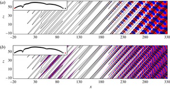
(view from below). Three periods of the domain are shown with positive and negative values coloured in red and blue, respectively, and contours of the streamwise baseflow component in black. The insets in the upper left corners indicate which mode in the spectrum is plotted.

For the cases C–E all the obtained eigenfunctions resemble a
 $z$
-type mode (Högberg & Henningson Reference Högberg and Henningson1998; Malik et al.
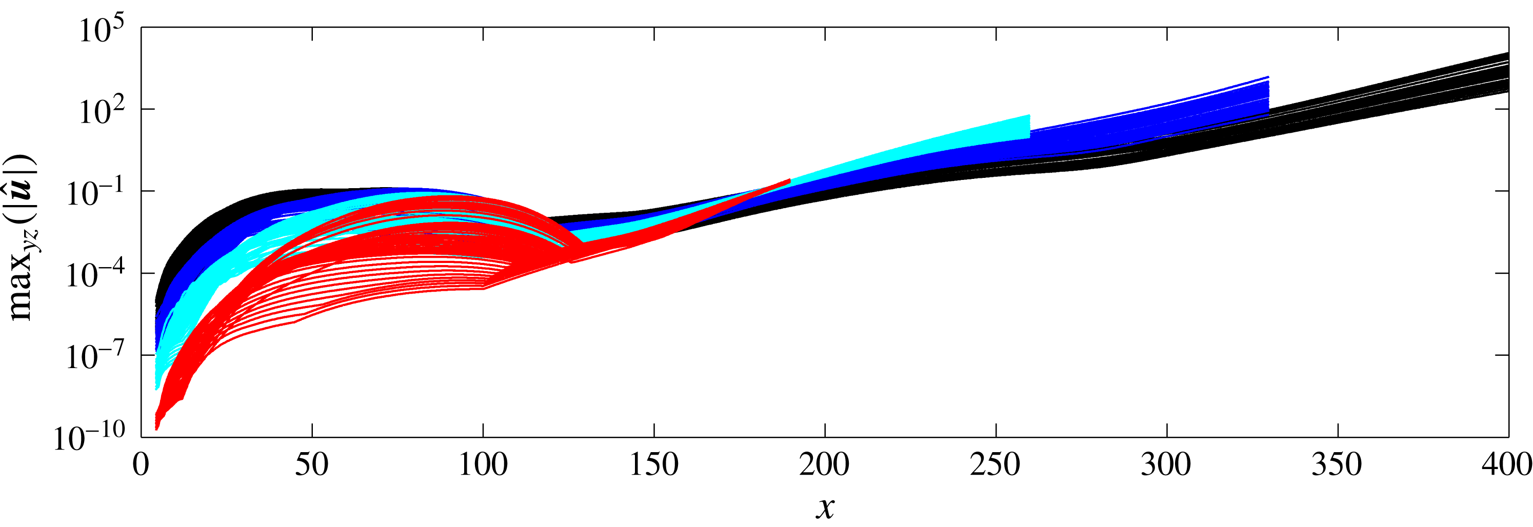
Reference Malik, Li, Choudhari and Chang1999) shown in figure 7. The spanwise maximum modulus of all the eigenfunctions is plotted in figure 8. The eigenfunctions consist of two different regions of spatial growth – one located immediately behind the roughness and extending to
 $x\approx 120$
, and another region that coincides with the growth of the CF vortices and extends up to the sponge region. Comparison of figure 8 with figure 29 in Kurz & Kloker (Reference Kurz and Kloker2016) shows that their eigenfunctions mainly consist of the first region, whereas the second region, which according to figure 8 becomes dominant for longer domains, has been truncated in their analysis. This could explain why their growth rates did not change significantly with the length of their rather short domains.
As seen in figure 9, the strength of the first upstream region increases with frequency. A close-up of the vortical structures and the eigenfunctions in the vicinity of the roughness (figure 10) reveals that these evolve around the central vortex ‘2’ developing from the recirculation region behind the roughness. For the high-frequency
 $z$
modes, the eigenfunctions in this region consist of narrow structures with a short spatial wavelength that are inclined against the direction of the baseflow. The relatively low amplitude of this region for the low-frequency
 $z$
modes plotted in figures 9(a) and 10(a), compared to the corresponding region for the high-frequency
 $z$
modes (figures 9
b and 10
b), might be related to the longer spatial wavelengths associated with the low-frequency
 $z$
modes. These eigenfunctions are normalised to have unit energy in the domain
 $\unicode[STIX]{x1D6FA}^{D}$
.
Regarding the eigenfunctions in cases A and B, the identification of
 $z$
modes is less clear, due to the low amplitude of the CF vortices in these cases. Notable is that some low-frequency and stationary modes appear in the eigenvalue spectra for these cases (figure 6). However, these are all stable and not associated with the transition and global instability of the flow.
Location of the eigenfunctions plotted in figure 9 relative to the vortex structures developing from the roughness near-wake into the far-wake CF vortices. The vortex structures are shown with the
 $\unicode[STIX]{x1D706}_{2}$
-criterion (Jeong & Hussain Reference Jeong and Hussain1995) in green, and positive and negative values of the eigenfunctions are coloured in red and blue, respectively. For visualisation purposes, the contour levels of the eigenfunctions in panel (a) are 10 times smaller than those in panel (b).

3.3 Structural sensitivity
Parameter variations such as those presented in the previous sections can be interpreted as structural perturbations to the governing operator. The concept of structural sensitivity analysis was introduced by Giannetti & Luchini (Reference Giannetti and Luchini2007) and aims to identify the spatial regions of the flow where a forcing or a modification of the set-up yields the largest change in an eigenvalue. By considering the sensitivity of an eigenvalue to a spatially localised force–velocity coupling, the eigenvalue drift due to a structural perturbation may be bounded by the product between the direct and adjoint eigenfunctions,
 $$\begin{eqnarray}\unicode[STIX]{x1D707}(\boldsymbol{x})=\frac{\Vert \hat{\boldsymbol{u}}^{\dagger }(\boldsymbol{x})\Vert \Vert \hat{\boldsymbol{u}}(\boldsymbol{x})\Vert }{\displaystyle \int _{\unicode[STIX]{x1D6FA}}|\hat{\boldsymbol{u}}^{\dagger }\boldsymbol{\cdot }\hat{\boldsymbol{u}}|\,\text{d}\unicode[STIX]{x1D6FA}},\end{eqnarray}$$
subject to the normalisation
 $\max _{\boldsymbol{x}\in \unicode[STIX]{x1D6FA}}\{|\hat{u} (\boldsymbol{x})|\}=1$
(Giannetti & Luchini denotes this quantity by
 $\unicode[STIX]{x1D706}$
). Regions of the flow where
 $\unicode[STIX]{x1D707}$
is non-zero indicate locations that are sensitive to forcing.
The adjoint eigenfunction
 $\hat{\boldsymbol{u}}^{\dagger }$
appearing in (3.1) is here obtained by determining the eigenfunctions of the discretised adjoint Navier–Stokes equations (Hill Reference Hill1995)
 $$\begin{eqnarray}\displaystyle -\frac{\unicode[STIX]{x2202}\boldsymbol{u}^{\dagger }}{\unicode[STIX]{x2202}t}-(\boldsymbol{U}\boldsymbol{\cdot }\unicode[STIX]{x1D735})\boldsymbol{u}^{\dagger }+(\unicode[STIX]{x1D735}\boldsymbol{U})^{\text{T}}\boldsymbol{u}^{\dagger } & = & \displaystyle -\unicode[STIX]{x1D735}p^{\dagger }+\frac{1}{Re_{\unicode[STIX]{x1D6FF}_{0}^{\ast }}}\unicode[STIX]{x1D6FB}^{2}\boldsymbol{u}^{\dagger }+\boldsymbol{f}^{\dagger }\quad \text{in }\unicode[STIX]{x1D6FA},\end{eqnarray}$$
 $$\begin{eqnarray}\displaystyle \unicode[STIX]{x1D735}\boldsymbol{\cdot }\boldsymbol{u}^{\dagger } & = & \displaystyle 0\quad \text{in }\unicode[STIX]{x1D6FA},\end{eqnarray}$$
 $_{us}$
in table 1). This minor modification does not significantly alter the details of the direct spectrum compared to that presented for case D in figure 5, and the direct and adjoint spectra are seen to match, although they do not exactly coincide (as can be expected due to their demonstrated sensitivity). The function
 $\unicode[STIX]{x1D707}$
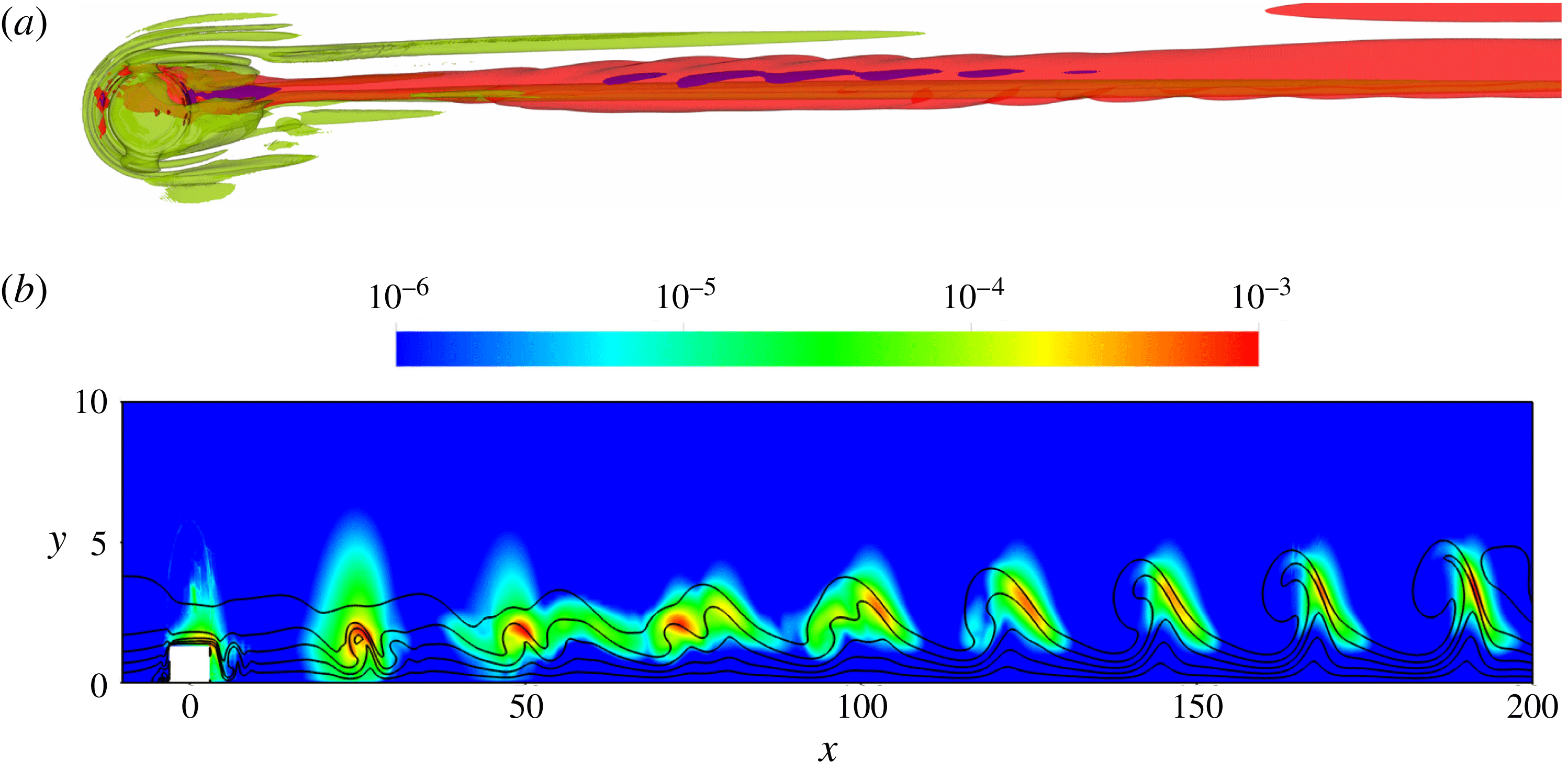
is evaluated using an eigenfunction whose eigenvalue is located in the middle of the branch, together with the adjoint eigenfunction corresponding to the closest adjoint eigenvalue. The resulting product is shown in figure 11. As seen in figure 11(a),
 $\unicode[STIX]{x1D707}$
is emphasised around the windward side of the roughness and the reversed flow region immediately behind the roughness. From there, the region of structural sensitivity develops along vortex ‘2’ in § 2.4 and extends throughout the entire domain as shown in figure 11(b). This can be contrasted with the corresponding distribution for the sinuous and varicose instability reported by Loiseau et al. (Reference Loiseau, Robinet, Cherubini and Leriche2014) and the leading eigenmode reported by Citro et al. (Reference Citro, Giannetti, Luchini and Auteri2015) for a roughness in a Blasius boundary layer, which were localised/emphasised in the reversed flow region behind the roughness.
Structural sensitivity: (a) iso-contours corresponding to
 $\unicode[STIX]{x1D707}=0.0001$
(red) and
 $\unicode[STIX]{x1D707}=0.001$
(blue) together with vortex structures visualised with the
 $\unicode[STIX]{x1D706}_{2}$
-criterion (Jeong & Hussain Reference Jeong and Hussain1995) (green); (b) the distribution of
 $\unicode[STIX]{x1D707}$
in the
 $xy$
-plane at
 $z=0$
together with contours of the streamwise baseflow component in black (note that the scaling on the vertical axis is enlarged for clarity).

Following the argument of Giannetti & Luchini (Reference Giannetti and Luchini2007), the effect of increasing the computational domain may be viewed as changing the boundary condition of the flow. They found that the eigenvalue only varied significantly when the boundary conditions were placed in the vicinity of the region where
 $\unicode[STIX]{x1D707}$
was notably different from zero. However, in their study (3.1) was evaluated for an eigenmode whose
 $\unicode[STIX]{x1D707}$
-distribution was localised in space, thus making it possible to enclose in a sufficiently large domain. For the present flow case, this does not seem to be possible (equation (3.1) evaluated for pairs of direct and adjoint eigenfunctions at the two ends of the branch give the same conclusion), which explains the trend seen in figure 6.
3.4 Impulse response
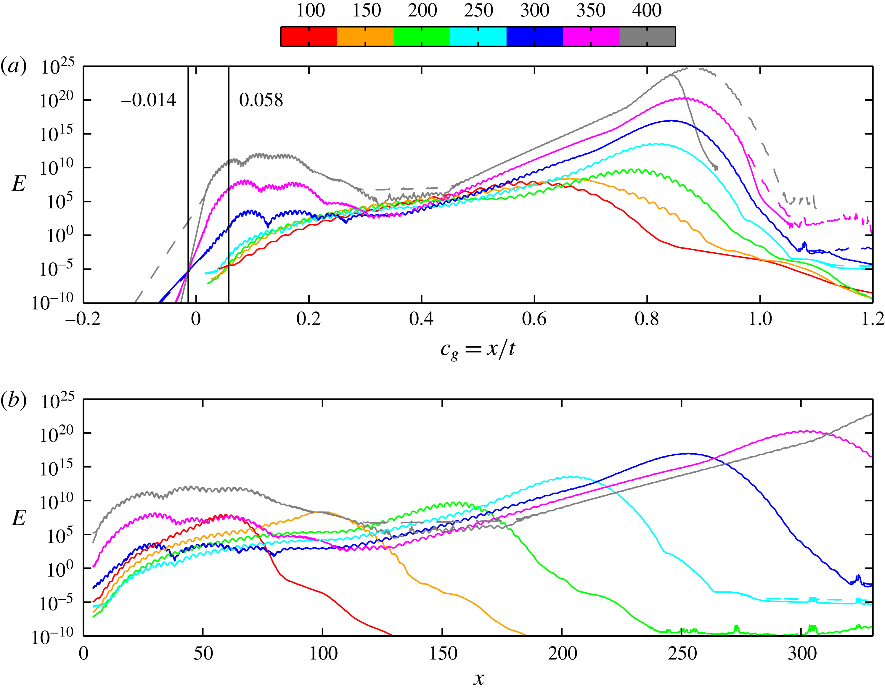
The energy of the wavepacket integrated over spanwise planes for different times (colour) as a function of (a) group velocity
 $c_{g}=x/t$
and (b) position
 $x$
, for the cases D (——) and E (– – – –). The vertical solid lines in (a) show trailing edge velocities
 $c_{g}^{-}$
for
 $t\leqslant 200$
and
 $t\geqslant 300$
.

In order to analyse the noted domain dependency in greater detail, an impulse-response analysis similar to those performed by Brandt et al. (Reference Brandt, Cossu, Chomaz, Huerre and Henningson2003) and Peplinski et al. (Reference Peplinski, Schlatter and Henningson2015) is carried out for cases D and E. As initial perturbation, a wavepacket-like disturbance (see Bech, Henningson & Henkes Reference Bech, Henningson and Henkes1998) is chosen that is oriented in the direction of the inviscid streamline and placed upstream of the roughness. If a flow is convectively unstable, disturbances are advected away from the location of initiation such that the flow in the limit of long times relaxes to its original state. In contrast, if the flow is absolutely or globally unstable, disturbances will regenerate at their initial location and grow in amplitude while they spread in the upstream and downstream directions. Hence, for a convectively unstable flow the trailing edge velocity of the wavepacket is positive, whereas for an absolutely or globally unstable flow, it is non-positive (Schmid & Henningson Reference Schmid and Henningson2001).
In figure 12(a) the energy of the wavepacket is plotted against the group velocity
 $c_{g}=x/t$
. As shown, the evolution of the impulse is similar for cases D and E (the lines are nearly indistinguishable), until the wavepacket in case D reaches the sponge region and gets dampened. By examining the intersection of the curves at the rear and front of the wavepacket at different times, the trailing and the leading edge velocity (
 $c_{g}^{-}$
and
 $c_{g}^{+}$
) of the wavepacket can be estimated. Initially, for
 $t\leqslant 200$
, this intersection gives
 $c_{g}^{-}\approx 0.058$
, which suggests that the flow is convectively unstable (i.e. globally stable) and the wavepacket will be advected out of the domain. This is, however, not the case for larger times. Extrapolating a least-squares fit to the energy curves for
 $t\geqslant 300$
and
 $x\leqslant 6.8$
yields
 $c_{g}^{-}\approx -0.014$
, which implies that the flow is globally unstable. As is evident from figure 12(b), this change in trailing edge velocity occurs when the wavepacket reaches the region of strong CF vortices (cf. figure 2). From figure 12(a) no well-defined leading edge
 $c_{g}^{+}$
can be determined, which is most likely due to the fact that the flow accelerates and the wavepacket propagates along the curved CF vortices.
The behaviour of the wavepacket is in line with figure 6 and confirms that there is a changeover to global instability as stronger CF vortices are included in the domain. The reason for this is the connection between the roughness near-wake and the far-wake CF depicted by the eigenfunctions in figure 8. As the energy of the wavepacket is amplified by the secondary unstable CF vortices in the far wake, the energy level in the near wake also increases. This alters the evolution of the wavepacket, which starts to spread also in the upstream direction. For even longer times, the amplitude in the far wake becomes so large that the connection between the near- and far-wake CF becomes impossible to resolve using double-precision arithmetic. A related effect can be seen at
 $t=400$
for case E in figure 12 as a flat middle region corresponding to the noise level set by the solver tolerance (
 $10^{-10}$
). At this point the tail of the wavepacket is below this noise level and changes slope, which implies that flow physics is erroneously represented. Given this result, further increases in domain size will be questionable.
3.5 Energy budget
To gain further insight into the quantities most sensitive to domain size, an analysis of the energy budget is carried out. The computed eigenfunctions are substituted into the linearised evolution equation for the kinetic perturbation energy (Schmid & Henningson Reference Schmid and Henningson2001),
 $$\begin{eqnarray}u_{l}\frac{\unicode[STIX]{x2202}u_{l}}{\unicode[STIX]{x2202}t}=-u_{l}u_{j}\frac{\unicode[STIX]{x2202}U_{l}}{\unicode[STIX]{x2202}x_{j}}-\frac{1}{Re_{\unicode[STIX]{x1D6FF}_{0}^{\ast }}}\frac{\unicode[STIX]{x2202}u_{l}}{\unicode[STIX]{x2202}x_{j}}\frac{\unicode[STIX]{x2202}u_{l}}{\unicode[STIX]{x2202}x_{j}}+\frac{\unicode[STIX]{x2202}}{\unicode[STIX]{x2202}x_{j}}\left(-\frac{1}{2}u_{l}u_{l}U_{j}-u_{l}p\unicode[STIX]{x1D6FF}_{lj}+\frac{1}{Re_{\unicode[STIX]{x1D6FF}_{0}^{\ast }}}u_{l}\frac{\unicode[STIX]{x2202}u_{l}}{\unicode[STIX]{x2202}x_{j}}\right)\quad \text{in }\tilde{\unicode[STIX]{x1D6FA}},\end{eqnarray}$$
where
 $j,l\in \{1,2,3\}$
, upon which an expression for the growth rate
 $\unicode[STIX]{x1D714}_{i}$
can be derived as
 $$\begin{eqnarray}\unicode[STIX]{x1D714}_{i}=\frac{1}{E_{\tilde{\unicode[STIX]{x1D6FA}}}}\int _{\tilde{\unicode[STIX]{x1D6FA}}}({\mathcal{P}}-{\mathcal{E}}+{\mathcal{T}}+\unicode[STIX]{x1D6F1}+{\mathcal{D}})\,\text{d}\unicode[STIX]{x1D6FA}.\end{eqnarray}$$
In (3.4),
 $E_{\tilde{\unicode[STIX]{x1D6FA}}}=\int _{\tilde{\unicode[STIX]{x1D6FA}}}(\hat{u} _{j}^{r2}+\hat{u} _{j}^{i2})\,\text{d}\unicode[STIX]{x1D6FA}$
represents the kinetic energy in
 $\tilde{\unicode[STIX]{x1D6FA}}$
(superscript
 $r$
and
 $i$
refer to the real and imaginary parts of the eigenfunctions). The terms on the right-hand side of (3.4) read
 $$\begin{eqnarray}\left.\begin{array}{@{}c@{}}{\mathcal{P}}=-(\hat{u} _{l}^{r}\hat{u} _{j}^{r}+\hat{u} _{l}^{i}\hat{u} _{j}^{i}){\displaystyle \frac{\unicode[STIX]{x2202}U_{l}}{\unicode[STIX]{x2202}x_{j}}},\quad {\mathcal{E}}={\displaystyle \frac{1}{Re_{\unicode[STIX]{x1D6FF}_{0}^{\ast }}}}\left[\left({\displaystyle \frac{\unicode[STIX]{x2202}\hat{u} _{l}^{r}}{\unicode[STIX]{x2202}x_{j}}}\right)^{2}+\left({\displaystyle \frac{\unicode[STIX]{x2202}\hat{u} _{l}^{i}}{\unicode[STIX]{x2202}x_{j}}}\right)^{2}\right],\\ {\mathcal{T}}=-\left(\hat{u} _{l}^{r}{\displaystyle \frac{\unicode[STIX]{x2202}\hat{u} _{l}^{r}}{\unicode[STIX]{x2202}x_{j}}}+\hat{u} _{l}^{i}{\displaystyle \frac{\unicode[STIX]{x2202}\hat{u} _{l}^{i}}{\unicode[STIX]{x2202}x_{j}}}\right)U_{j},\quad \unicode[STIX]{x1D6F1}=-\left(\hat{u} _{l}^{r}{\displaystyle \frac{\unicode[STIX]{x2202}\hat{p}^{r}}{\unicode[STIX]{x2202}x_{j}}}+\hat{u} _{l}^{i}{\displaystyle \frac{\unicode[STIX]{x2202}\hat{p}^{i}}{\unicode[STIX]{x2202}x_{j}}}\right)\unicode[STIX]{x1D6FF}_{lj},\\ {\mathcal{D}}={\displaystyle \frac{1}{Re_{\unicode[STIX]{x1D6FF}_{0}^{\ast }}}}\left[\left({\displaystyle \frac{\unicode[STIX]{x2202}\hat{u} _{l}^{r}}{\unicode[STIX]{x2202}x_{j}}}\right)^{2}+\hat{u} _{l}^{r}{\displaystyle \frac{\unicode[STIX]{x2202}^{2}\hat{u} _{l}^{r}}{\unicode[STIX]{x2202}x_{j}\unicode[STIX]{x2202}x_{j}}}+\left({\displaystyle \frac{\unicode[STIX]{x2202}\hat{u} _{l}^{i}}{\unicode[STIX]{x2202}x_{j}}}\right)^{2}+\hat{u} _{l}^{i}{\displaystyle \frac{\unicode[STIX]{x2202}^{2}\hat{u} _{l}^{i}}{\unicode[STIX]{x2202}x_{j}\unicode[STIX]{x2202}x_{j}}}\right],\end{array}\right\}\end{eqnarray}$$
and correspond to production (
 ${\mathcal{P}}$
) and dissipation (
 ${\mathcal{E}}$
) of energy and transport of energy by advection (
 ${\mathcal{T}}$
), pressure perturbation (
 $\unicode[STIX]{x1D6F1}$
) and diffusion (
 ${\mathcal{D}}$
). Comparison of the growth rates given by the global stability analysis to those obtained by integrating (3.4)–(3.5) over
 $\tilde{\unicode[STIX]{x1D6FA}}^{D}$
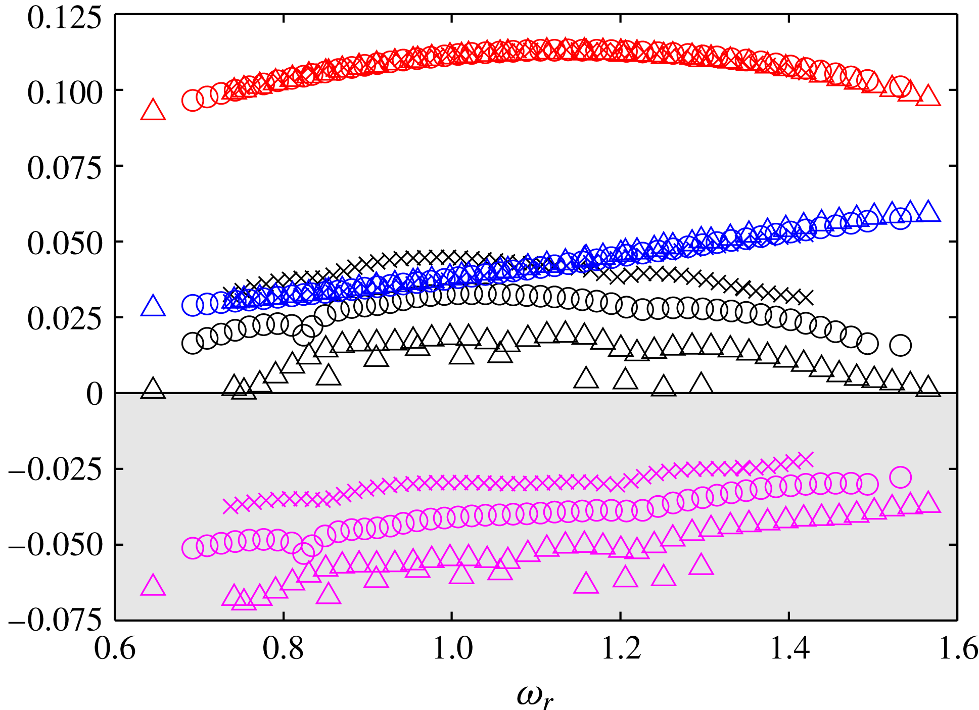
for case D shows excellent agreement (see figure 6).
By including the minus sign in the definition of
 ${\mathcal{P}}$
, its interpretation becomes analogous to that of the corresponding term in a turbulent kinetic energy budget. Thus, gradients of the baseflow working against the velocity perturbations withdraw energy from the baseflow and transfer it to the perturbation field. The term
 ${\mathcal{E}}$
accounts for dissipation of kinetic energy by viscosity and is always non-negative. The transport terms represent spatial redistribution of energy, and through application of the Gauss theorem these may be interpreted as energy fluxes over the domain boundaries. If the perturbations are assumed to be localised or spatially periodic, these transport terms vanish when integrating over the domain.
Focusing on the longer domains (the cases C–E) and choosing
 $\tilde{\unicode[STIX]{x1D6FA}}^{C}$
as the domain of integration, the terms in (3.4) that mainly contribute to the growth rates are identified to be production, dissipation and advection, whereas other terms are orders of magnitude smaller. It is seen in figure 13 that production (red) and dissipation (blue) of energy nearly coincide for all three cases, and that the entire change in growth rate can be attributed to a decrease in the advection rate of perturbation energy by the baseflow (magenta). As
 $\int _{\tilde{\unicode[STIX]{x1D6FA}}^{C}}{\mathcal{T}}/E_{\tilde{\unicode[STIX]{x1D6FA}}^{C}}\,\text{d}\unicode[STIX]{x1D6FA}$
decreases, energy will be transported out of the domain at a lower rate, which explains the higher growth rates.
Energy budget of the cases C (▵), D (○) and E (
 $\times$
) showing
 ${\mathcal{P}}$
(red),
 ${\mathcal{E}}$
(blue) and
 ${\mathcal{T}}$
(magenta) integrated over
 $\tilde{\unicode[STIX]{x1D6FA}}^{C}$
and normalised by
 $E_{\tilde{\unicode[STIX]{x1D6FA}}^{C}}$
, together with the growth rates (black).

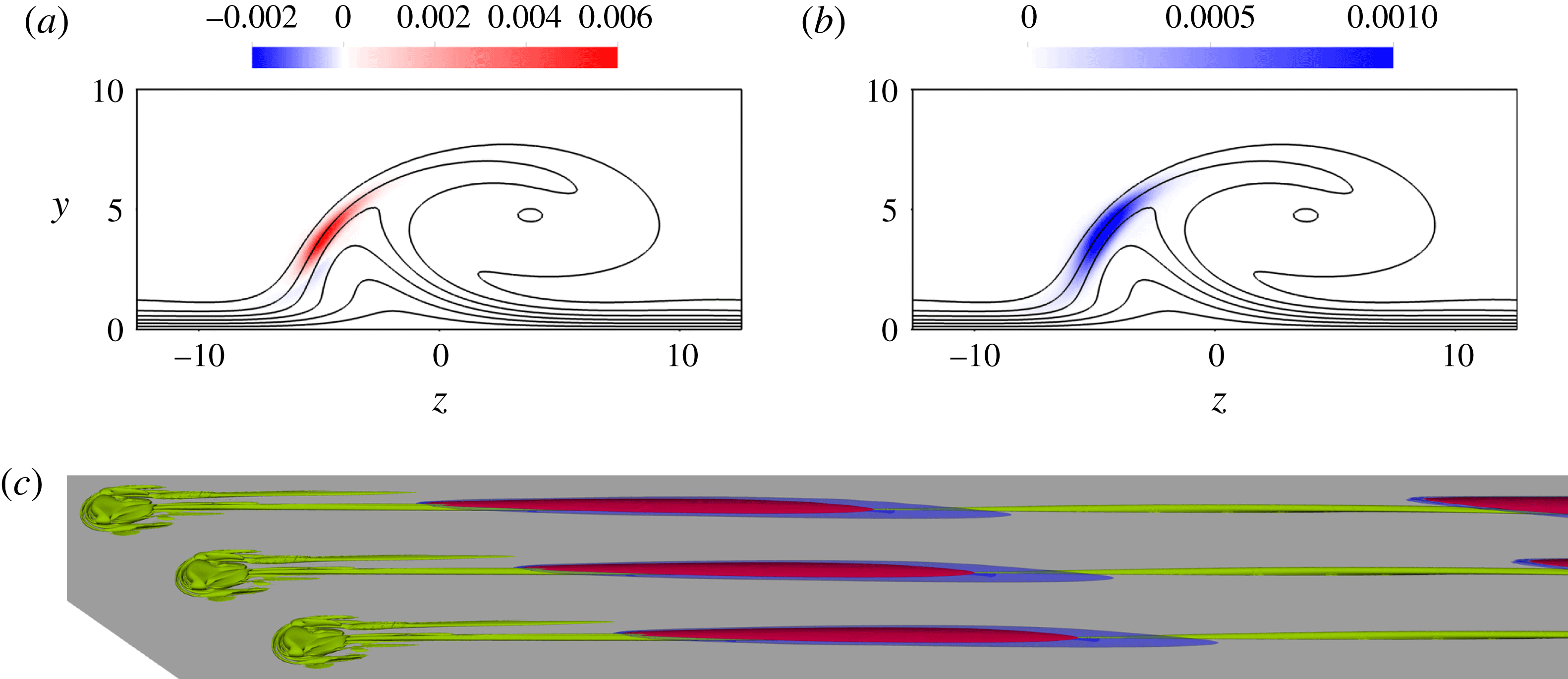
Energy production (
 ${\mathcal{P}}/E_{\tilde{\unicode[STIX]{x1D6FA}}^{D}}$
) and dissipation (
 ${\mathcal{E}}/E_{\tilde{\unicode[STIX]{x1D6FA}}^{D}}$
) for the eigenmode shown in figures 9(b) and 10(b). Panels (a) and (b) show the location relative to the CF vortex of
 ${\mathcal{P}}/E_{\tilde{\unicode[STIX]{x1D6FA}}^{D}}$
and
 ${\mathcal{E}}/E_{\tilde{\unicode[STIX]{x1D6FA}}^{D}}$
, respectively, at the streamwise position
 $x=327$
(view from upstream); (c) shows the iso-contour of
 ${\mathcal{P}}/E_{\tilde{\unicode[STIX]{x1D6FA}}^{D}}$
corresponding to
 $10^{-9}$
(red) and the iso-contour of
 ${\mathcal{E}}/E_{\tilde{\unicode[STIX]{x1D6FA}}^{D}}$
corresponding to
 $10^{-10}$
(blue) in the near wake together with the vortex structures of the baseflow visualised with the
 $\unicode[STIX]{x1D706}_{2}$
-criterion (Jeong & Hussain Reference Jeong and Hussain1995) (green).

Since
 $\int _{\tilde{\unicode[STIX]{x1D6FA}}^{C}}{\mathcal{P}}/E_{\tilde{\unicode[STIX]{x1D6FA}}^{C}}\,\text{d}\unicode[STIX]{x1D6FA}$
and
 $\int _{\tilde{\unicode[STIX]{x1D6FA}}^{C}}{\mathcal{E}}/E_{\tilde{\unicode[STIX]{x1D6FA}}^{C}}\,\text{d}\unicode[STIX]{x1D6FA}$
are seen to be roughly the same for the different cases, the spatial structures of
 ${\mathcal{P}}$
and
 ${\mathcal{E}}$
are investigated in more detail. As shown in figure 14, the region of non-zero production and dissipation is not localised but distributed across the whole domain. Downstream in the far wake (figure 14
a), the region where the production is positive aligns with the frontal region of the CF vortices, similarly to what was found by Malik et al. (Reference Malik, Li, Choudhari and Chang1999) considering solely the dominant production term (compare with their figure 10). Plotting the dissipation, as is done in figure 14(b), shows that the same region is also responsible for dissipating energy. In the upstream region, figure 14(c) shows that the production and dissipation of perturbation energy is confined to the central vortex ‘2’ along which the eigenmode evolves. In figure 14,
 ${\mathcal{P}}/E_{\tilde{\unicode[STIX]{x1D6FA}}^{D}}$
and
 ${\mathcal{E}}/E_{\tilde{\unicode[STIX]{x1D6FA}}^{D}}$
are shown for the high-frequency
 $z$
mode plotted in figures 9(b) and 10(b). The corresponding structures for the low-frequency
 $z$
mode in figures 9(a) and 10(a) have a similar shape and location, although the magnitude of these quantities in the near wake are orders of magnitude lower than for the high-frequency mode.
4 Discussion and conclusion
It is shown in this paper that a FSC boundary layer with a roughness element large enough to excite cross-flow vortices, but small enough to avoid an immediate flow tripping, is globally unstable if sufficiently strong CF vortices are induced in the domain. The corresponding eigenvalue spectra feature an eigenvalue branch, which is very sensitive to numerical parameters. Study of the approximate
 $\unicode[STIX]{x1D700}$
-pseudospectrum (Toh & Trefethen Reference Toh and Trefethen1996) shows that a minute change in the set-up, e.g. solver tolerance, can move the eigenvalues from a level of
 $\unicode[STIX]{x1D700}\sim 10^{-8}$
to
 $\unicode[STIX]{x1D700}\sim 10^{-5}$
. Such sensitivity implies that it is impossible to determine a unique converged set of eigenvalues for this flow. The growth rates of the eigenmodes also increase with domain size due to the inclusion of stronger CF vortices, and a structural sensitivity analysis reveals that the region of structural sensitivity is distributed throughout the entire domain. The increase in growth rate with domain size is reflected in the energy budget as a decrease in the advection rate of perturbation energy by the baseflow. An impulse-response analysis suggests that there is a changeover from convective to global instability as stronger CF vortices are included in the domain.
These results are consistent with the nonlinear DNS. As shown in figure 8, the difference in amplitude of the eigenfunction between the near- and far-wake regions is several orders of magnitude. In a nonlinear DNS, the amplitudes of the modes saturate at finite values due to nonlinearities. Since the two regions are connected, transition in the far wake will prevent the eigenfunctions from growing in the near wake and therefore keep the transition point from moving upstream towards the roughness. Although the aim of this article is not to enter a discussion about the nonlinear phenomena of the flow, subtracting the baseflow from the DNS field visualised in figure 3(b) reveals the presence of a locally amplified wave in the near wake (figure 15). These structures are very similar to the eigenfunctions shown in figure 10, and spectral analysis of a probe signal measured in this region reveals a band of amplified frequencies between approximately 0.8 and 2.1, which agrees with the reported eigenvalue spectra. This indicates that the unstable global modes reported herein are indeed responsible for transition seen in the nonlinear DNS, and emphasises the need for including both the near- and far-wake parts of the eigenfunctions in the domain in order to deduce the correct behaviour of the flow.
Visualisation of the unsteady wave structure found by subtracting the steady baseflow from the nonlinear DNS shown in figure 3(b) (
 $k=1.3$
,
 $Re_{k}=458.01$
). Red and blue colours correspond to positive and negative streamwise velocities, respectively, and vortex structures of the baseflow are visualised with the
 $\unicode[STIX]{x1D706}_{2}$
-criterion (Jeong & Hussain Reference Jeong and Hussain1995) in green.

It is notable that the change in domain size mainly affects the growth rates of the modes and to a lesser extent their frequencies (see figure 6). This suggests that the frequency spectrum of the flow is determined by the near wake, and that the far wake, which is dominated by the CF vortices, mainly acts as an amplifier that is driven by the near-wake behaviour and has little influence on the frequency selection. However, since the eigenfunctions are seen to extend over both of these regions, such an interaction between the near and far wake does not require the near wake to be an oscillator on its own, as shown. It is emphasised that this feedback between the near and far wake is physical and therefore not to be confused with a spurious pressure feedback from the outflow boundary, which can give rise to similar domain dependency and shape of the spectrum/
 $\unicode[STIX]{x1D700}$
-pseudospectrum (Lesshafft Reference Lesshafft2017). Unstable eigenvalue branches analogous to those reported herein have for instance also been observed in flows without inflow and outflow boundaries such as toroidal pipes with small curvature (Canton, Schlatter & Örlü Reference Canton, Schlatter and Örlü2016).
Regarding the comparison of the flow phenomena observed in the FSC boundary layer with those in a Blasius boundary layer, several similarities and differences prevail. In both cases, vortices developing in the vicinity of the roughness induce high- and low-speed streaks downstream of the recirculation region. If the roughness elements in a Blasius boundary layer are isolated, the eigenfunctions will be localised around the central low-speed streak, from which both the sinuous and the varicose instabilities mainly extract energy (Loiseau et al. Reference Loiseau, Robinet, Cherubini and Leriche2014). Since these structures eventually decay, the region in space from which the perturbation can extract energy is limited, and hence the perturbation ultimately also has to decay. As a result, the onset of global instability in this case corresponds to an instability of the near wake, which yields an immediate flow tripping behind the roughness. For the FSC boundary layer, the perturbation is likewise seen to evolve around and withdraw energy from the vortical structure associated with the central low-speed streak. However, instead of decaying, this streak merges with another low-speed streak and a CF vortex develops, which enables the perturbation to extract energy over the whole domain. This causes the onset of global instability to involve not only the near wake but the entire flow field. If the far wake is excluded from the domain, this energy extraction from the far-wake baseflow structures to the perturbation will be absent. Therefore an eigenmode in a short domain that is restricted to the near wake will be globally stable, as shown by the global stability analysis of case A.
A possible way to overcome the issue with domain dependency would be to introduce a variable pressure gradient that dampens the CF vortices. For the constant pressure gradient boundary layer, on the other hand, a question is whether the growth rates will increase unboundedly with the length of the domain. In the case of longer domains, even stronger CF vortices will be included, whose amplitudes eventually will saturate. Given the budget in § 3.5, it seems unphysical that
 $\int _{\tilde{\unicode[STIX]{x1D6FA}}^{C}}{\mathcal{T}}/E_{\tilde{\unicode[STIX]{x1D6FA}}^{C}}\,\text{d}\unicode[STIX]{x1D6FA}$
will change sign for a sufficiently long domain, since that might imply that the baseflow will change direction. Hence, if the mode shape remains unchanged and the results in figure 13 continue to hold, such that
 $\int _{\tilde{\unicode[STIX]{x1D6FA}}^{C}}{\mathcal{T}}/E_{\tilde{\unicode[STIX]{x1D6FA}}^{C}}\,\text{d}\unicode[STIX]{x1D6FA}\rightarrow 0$
as
 $\tilde{x}_{max}\rightarrow \infty$
, an upper bound for the growth rates can be estimated to be
 $\unicode[STIX]{x1D714}_{i}\approx 0.074$
.
Acknowledgements
We thank Dr A. Peplinski for discussions and for providing some of the tools used. Professor P. Schmid and Dr D. Sipp are acknowledged for valuable discussions. Simulations were performed at the National Supercomputer Centre (NSC) and PDC Center for High Performance Computing in Sweden with computer time granted by the Swedish National Infrastructure for Computing (SNIC).
Appendix A. Falkner–Skan–Cooke similarity solution
The similarity solutions of Falkner & Skan (Reference Falkner and Skan1931) and Cooke (Reference Cooke1950), subject to boundary conditions
 $f=f^{\prime }=g=0$
at
 $\unicode[STIX]{x1D702}=0$
and
 $f^{\prime }\rightarrow 1$
,
 $g\rightarrow 1$
as
 $\unicode[STIX]{x1D702}\rightarrow \infty$
, are given by
 $$\begin{eqnarray}\displaystyle & f^{\prime \prime \prime }+ff^{\prime \prime }+\unicode[STIX]{x1D6FD}_{H}(1-{f^{\prime }}^{2})=0, & \displaystyle\end{eqnarray}$$
 $$\begin{eqnarray}\displaystyle & g^{\prime \prime }+fg^{\prime }=0, & \displaystyle\end{eqnarray}$$
where
 $f^{\prime }(\unicode[STIX]{x1D702})$
and
 $g(\unicode[STIX]{x1D702})$
describe the velocity distributions in
 $x$
- and
 $z$
-directions, respectively, and
 $\unicode[STIX]{x1D6FD}_{H}=2m/(m+1)$
is the Hartree parameter. These equations are derived from Prandtl’s boundary layer equations (see Schlichting Reference Schlichting1979) and are solved with a shooting method using Newton–Raphson and fourth-order Runge–Kutta. Following Schlichting (Reference Schlichting1979), a streamfunction
 $\unicode[STIX]{x1D713}^{\ast }$
and a dimensionless wall-normal coordinate
 $\unicode[STIX]{x1D702}$
can be defined as
 $$\begin{eqnarray}\unicode[STIX]{x1D713}^{\ast }=\sqrt{\frac{2}{m+1}x^{\ast }U_{\infty }^{\ast }\unicode[STIX]{x1D708}^{\ast }}f,\quad u^{\ast }=\frac{\unicode[STIX]{x2202}\unicode[STIX]{x1D713}^{\ast }}{\unicode[STIX]{x2202}y^{\ast }},\quad v^{\ast }=-\frac{\unicode[STIX]{x2202}\unicode[STIX]{x1D713}^{\ast }}{\unicode[STIX]{x2202}x^{\ast }},\end{eqnarray}$$
 $$\begin{eqnarray}\unicode[STIX]{x1D702}=y^{\ast }\sqrt{\frac{m+1}{2}\frac{U_{\infty }^{\ast }}{\unicode[STIX]{x1D708}^{\ast }x^{\ast }}},\end{eqnarray}$$
from which the streamwise and wall-normal velocity components can be derived. These together with the spanwise velocity component read
 $$\begin{eqnarray}\displaystyle & \displaystyle U_{FSC}=U_{\infty }f^{\prime }, & \displaystyle\end{eqnarray}$$
 $$\begin{eqnarray}\displaystyle & \displaystyle V_{FSC}=\frac{1}{2}\sqrt{\frac{2}{m+1}\frac{U_{\infty }}{x}\frac{1}{Re_{\unicode[STIX]{x1D6FF}_{0}^{\ast }}}}\left[(1-m)f^{\prime }\unicode[STIX]{x1D702}-(1+m)f\right], & \displaystyle\end{eqnarray}$$
 $$\begin{eqnarray}\displaystyle & \displaystyle W_{FSC}=W_{\infty }g, & \displaystyle\end{eqnarray}$$
where
 $U_{\infty }(x)=(1+x/x_{0})^{m}$
and
 $W_{\infty }=W_{0}^{\ast }/U_{0}^{\ast }$
are given by (2.1) and (2.2), and
 $f^{\prime }$
,
 $f$
and
 $g$
are obtained from (A 1) and (A 2).