2. Overview of one-dimensional models for the class-averaged settling velocity

For a Stokesian suspension of polydisperse spheres grouped into $m$ distinct particle size classes, the average settling velocity of the $i$th class can be written as $\langle u_i \rangle = u_{St,i} h_i(\boldsymbol {\phi })$, where $u_{St,i}=({2}/{9\mu }) a_i^2 (\rho _p-\rho _f)g$ is the single-particle Stokes velocity of the $i$th class, $h_i(\boldsymbol {\phi })$ is the hindered settling function of that class and $\boldsymbol {\phi }=(\phi _1,\phi _2,\ldots,\phi _m)$ is the vector of volume fractions (Davis & Acrivos Reference Davis and Acrivos1985); $a_i$ is the particle radius, $\mu$ is the fluid viscosity and $\rho _p - \rho _f$ is the density difference between the particles and the fluid.

The literature reports several models for $h_i(\boldsymbol {\phi })$, as reviewed by Berres et al. (Reference Berres, Bürger and Tory2005). The only model that is completely based on first principles is the model of Batchelor (Reference Batchelor1982), which was developed as an extension of the former theory of Batchelor for monodisperse suspensions (Batchelor Reference Batchelor1972). Batchelor's formula reads

(2.1)\begin{equation} h_i(\boldsymbol{\phi})=1+\sum_{j=1}^{m} S_{ij}\phi_j, \end{equation}

where $S_{ij}$ are scalar sedimentation coefficients that are functions of the size ratio $a_i/a_j$ for spheres of identical mass density (Batchelor & Wen Reference Batchelor and Wen1982) (an explicit expression for $S_{ij}$ is given in § 5.2). Batchelor's model is accurate to first order in the total volume fraction $\phi = \sum _j \phi _j$ and is, therefore, in principle only valid for negligibly small values of $\phi$. A semi-empirical extension of Batchelor's formula was proposed by Davis & Gecol (Reference Davis and Gecol1994) to improve the predictive capability in the regime of relatively high volume fractions. Their formula reads

(2.2)\begin{equation} h_i(\boldsymbol{\phi})= (1-\phi)^{-S_{ii}} \left(1+\sum_{j=1}^{m} (S_{ij}-S_{ii})\phi_j \right), \end{equation}

where the coefficients $S_{ij}$ are defined as in (2.1). The model is essentially an interpolation formula between an exact result (for $\phi \rightarrow 0$, (2.2) recovers (2.1)) and an approximate result (in the dense limit, for $m=1$ equation (2.2) reduces to a power-law form, where the exponent $-S_{ii}=6.55$ is numerically close to the exponent $\simeq$5 of the well-known Richardson–Zaki formula). The models of Batchelor and Davis & Gecol have been tested in experiments and simulations of bidisperse suspensions (Davis & Birdsell Reference Davis and Birdsell1988; Al-Naafa & Selim Reference Al-Naafa and Selim1992; Abbas et al. Reference Abbas, Climent, Simonin and Maxey2006; Wang & Brady Reference Wang and Brady2015; Chen et al. Reference Chen, Jia, Fairweather and Hunter2023). In experiments, the descending velocities of the interfaces separating different regions were measured. In simulations, settling velocities of the two classes were calculated. It was shown that Batchelor's model works reasonably well for dilute suspensions with $\phi$ within 5 %, and Davis & Gecol's model can also be used for dense suspensions.

Models (2.1) and (2.2) are rarely used in practice because they contain a large number of coefficients. Simpler expressions have therefore been developed for practical predictions of the hindered settling of polydisperse suspensions. The most popular is the MLB model (Lockett & Bassoon Reference Lockett and Bassoon1979; Masliyah Reference Masliyah1979). The MLB model has been partially validated by comparison of predicted and experimentally measured concentration profiles following settling, starting at the initial time from a homogeneous suspension with a Gaussian particle size distribution (Xue & Sun Reference Xue and Sun2003; Berres et al. Reference Berres, Bürger and Tory2005). This validation is not complete because the particle concentration at a given point in space is the sum of the concentrations of the different particle classes. Therefore, if a range of the particle size distribution makes a dominant contribution to the concentration, then an acceptably accurate prediction of the concentration profile may hide errors in the prediction of the velocity of certain particle classes. Furthermore, validation of the settling rates predicted by the MLB model for more than three size classes has not been published.

The MLB model reads

(2.3)\begin{equation} h_i(\boldsymbol{\phi})= (1-\phi)^{n-1} \left(1-\sum_{j=1}^{m} \left(\frac{a_j}{a_i}\right)^2\phi_j \right), \end{equation}

where $a_j/a_i$ is the ratio of the radii of the $j$th and the $i$th species. Appendix A contains details of the derivation of the MLB model, so that the model assumptions can be evaluated. The function $(1-\sum _{j=1}^{m} ({a_j}/{a_i})^2\phi _j )$ is the hindered settling function obtained by including the effect of volume fraction on the fluid–solid slip velocity (a continuity effect), and neglecting the effect of hydrodynamic interactions on the drag force experienced by each particle. The prefactor $(1-\phi )^{n-1}$ incorporates the effect of hydrodynamic interactions.

An even simpler model, which has been adopted by some authors (Davis & Hassen Reference Davis and Hassen1988; Abeynaike et al. Reference Abeynaike, Sederman, Khan, Johns, Davidson and Mackley2012; Vowinckel et al. Reference Vowinckel, Withers, Luzzatto-Fegiz and Meiburg2019; Chen et al. Reference Chen, Jia, Fairweather and Hunter2023), is based on the model of Richardson & Zaki (Reference Richardson and Zaki1954) for monodisperse suspensions. It reads

(2.4)\begin{equation} h_i(\boldsymbol{\phi}) = (1-\phi)^n, \end{equation}

where $n \approx 5$ (Brzinski & Durian Reference Brzinski and Durian2018). This model predicts different velocities for different particle radii $a_i$, because $h_i$ contains the single-particle Stokes formula at denominator. In the current paper, this hindered settling formula is referred to as the Richardson–Zaki model for polydispersed suspensions.

3. Numerical approach and validation

Consider a polydisperse suspension of $N$ spheres having the same density but different radii. The $N$ spheres are divided into $m$ size classes. The radius of size class $i$ is $a_i$. Each sphere in class $i$ is subjected to a force $\boldsymbol {F}_i=\frac {4}{3} {\rm \pi}a_i^3 (\rho _p-\rho _f) \boldsymbol {g}$, which includes the particle weight and buoyancy; $\rho _p$ and $\rho _f$ are the densities of the spheres and the fluid, respectively, and $\boldsymbol {g}$ is the gravitational acceleration. 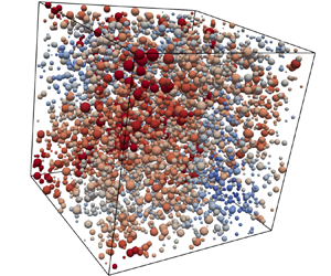The single-particle Stokes velocity corresponding to each class is $\boldsymbol {u}_{St,i}={2}/({9\mu }) a_i^2 (\rho _p-\rho _f)\boldsymbol {g}$, where $\mu$ is the dynamic viscosity of the fluid. In the current work, the particle velocity statistics are calculated from instantaneous random configuration of the spheres by first averaging over the particles in the computational domain and then ensemble-averaging over statistically identical configurations. Each configuration is generated by randomly placing the spheres one by one inside the computational domain, ensuring that each placement gives no overlap between the spheres (Revay & Higdon Reference Revay and Higdon1992; Wang & Brady Reference Wang and Brady2015; Cheng & Wachs Reference Cheng and Wachs2023a) (we note that a simulation of settling under gravity of a random particle configuration is different from a simulation of uniform flow past fixed random arrays, because in the former case different particles have different velocities, while in the latter the relative velocity between the particles and the undisturbed fluid is uniform). An example of a random array configuration is shown in figure 1. In our coordinate system, gravity is aligned in the $z$ direction, also referred to as the vertical direction in the following. The horizontal direction corresponds to the $x$ and $y$ coordinates.

Figure 1.

A configuration for volume fraction $\phi = 0.05$ and polydispersity parameter $\alpha = 0.4$. The spheres are coloured according to their radii.

To calculate the velocities of individual particles, a basic version of the Stokesian dynamics method is adopted (Brady et al. Reference Brady, Phillips, Lester and Bossis1988; Brady & Bossis Reference Brady and Bossis1988). While modern grid-based particle-resolved methods could be used (Willen & Prosperetti Reference Willen and Prosperetti2019; Yao, Criddle & Fringer Reference Yao, Criddle and Fringer2021; Shajahan & Breugem Reference Shajahan and Breugem2023), the Stokesian dynamics method is perfectly suitable for the objectives of the current paper: it is accurate in the relevant range of particle concentrations, it allows fast simulations and (unlike grid-based methods) it can simulate large ratios between the largest and smallest particle radii without numerical difficulties – a feature we would like to maintain for future highly polydisperse simulations. In the Stokesian dynamics method, the velocities of the spheres are calculated by solving the mobility problem

(3.1)\begin{equation} \boldsymbol{U}-\langle \boldsymbol{u} \rangle = \boldsymbol{\mathsf{M}} \boldsymbol{F}, \end{equation}

where $\boldsymbol {U}$ is the $3N$ vector containing the velocities of the spheres, $\boldsymbol {F}$ is the $3N$ vector containing the gravitational forces acting on the spheres (these forces include the particle weight and the buoyancy force) and $\boldsymbol{\mathsf{M}}$ is the $3N\times 3N$ mobility matrix (Kim & Karrila Reference Kim and Karrila2013). In (3.1), $\langle \boldsymbol {u} \rangle$ is the average translational velocity of the suspension. In our simulations $\langle \boldsymbol {u} \rangle = \boldsymbol {0}$ because of the zero volume flux condition of batch sedimentation (Berres et al. Reference Berres, Bürger and Tory2005). Note that in the current work only velocity–force coupling is considered, i.e. the stresslet and other force moments are not considered. Brady & Durlofsky (Reference Brady and Durlofsky1988) showed that in a sedimenting suspension the inclusion of the stresslet changes the settling rate negligibly. Because we work in the relatively dilute limit, short-range lubrication forces are also neglected.

The mobility matrix $\boldsymbol{\mathsf{M}}$ depends on the positions and radii of the spheres. We use the Rotne–Prager approximation for this term (Rotne & Prager Reference Rotne and Prager1969; Zuk et al. Reference Zuk, Wajnryb, Mizerski and Szymczak2014). This approximation has been shown to give accurate predictions of the sedimentation velocities of suspensions from dilute to relatively dense (Brady & Durlofsky Reference Brady and Durlofsky1988). Triply periodic boundary conditions are applied to the simulation box. The mobility matrix is constructed using the Ewald summation technique by splitting the mobility matrix into a real-space part and a wave-space part (Beenakker Reference Beenakker1986). Explicit formulae for the mobility matrix for a polydisperse suspension can be found in Beenakker (Reference Beenakker1986) and Hase & Powell (Reference Hase and Powell2001). As characteristic length and velocity scales, we choose the mean particle radius $\langle a \rangle$ and the single-particle Stokes velocity corresponding to $\langle a \rangle$. To make forces non-dimensional we use the effective weight of the mean particle, $\frac {4}{3} {\rm \pi}\langle a \rangle ^3 (\rho _p-\rho _f) g$.

In figure 2, numerical predictions for a single sphere in a triply periodic cubic box are plotted against Hasimoto's analytical solution (Hasimoto Reference Hasimoto1959) and the simulation results of Brady et al. (Reference Brady, Phillips, Lester and Bossis1988). The volume fraction of the simple cubic array is varied by varying the size of the box. Based on the point-force assumption, Hasimoto (Reference Hasimoto1959) derived $u/u_{St}=1-1.7601\phi ^{1/3}$ for $\phi \ll 1$, where $u_{St}$ is the Stokes velocity of the sphere. Brady et al. (Reference Brady, Phillips, Lester and Bossis1988) used Stokesian dynamics with different approximations for the mobility matrix. The results of Brady et al. (Reference Brady, Phillips, Lester and Bossis1988) shown in figure 2 correspond to simulations in the Rotne–Prager approximation. As seen from figure 2, our results match exactly those of Brady et al. (Reference Brady, Phillips, Lester and Bossis1988) and converge to Hasimoto's solution for $\phi \rightarrow 0$. This test validates our implementation of the Ewald summation for the periodic boundary conditions.

Figure 2.

Normalised settling velocity versus volume fraction for a simple cubic array of monodisperse spheres. The line is the point-force solution of Hasimoto (Reference Hasimoto1959). Upward triangles are the numerical results of Brady et al. (Reference Brady, Phillips, Lester and Bossis1988).

In figure 3, the normalised relative settling velocity is shown as a function of the normalised centre-to-centre distance between two unequal spheres with size ratios 2 and 5, respectively. In our simulations, the radius of the large sphere is fixed to $a_l=2$. The radius of the small sphere is $a_s=1$ and 0.4 for size ratios 2 and 5, respectively (these values are chosen because the largest radius is 2 and the largest size ratio is 5 in the polydisperse simulations analysed in this paper). The relative settling velocity between the two spheres is normalised by the Stokes velocity of the large sphere. The centre-to-centre distance is normalised by the radius of the large sphere. In figure 3, symbols are results from our simulations and lines correspond to the asymptotic solution of Wacholder & Sather (Reference Wacholder and Sather1974), in which only far-field hydrodynamic interactions were considered. It can be seen that our results match the analytical solution for both vertically and horizontally aligned pairs.

Figure 3.

Normalised relative settling velocity for a pair of spheres as a function of the centre-to-centre distance for (a) size ratio 2 and (b) size ratio 5. Results of current simulations are shown as symbols and analytical results of Wacholder & Sather (Reference Wacholder and Sather1974) (WS) are shown as lines.

The current paper discusses results for bidisperse suspensions and polydisperse suspensions with more than two classes, also comparing with the monodisperse case. For the monodisperse case, the radius of the spheres is $a=1$. For the bidisperse case, two size ratios are considered: $a_2/a_1 =2$ and 5. The radii of the small size classes are $a_1=0.8$ and 0.4 for these two size ratios, respectively. The volume fraction of the small size class is $\phi _1=\frac {3}{11}\phi$ for size ratio 2 and $\phi _1=\frac {1}{76}\phi$ for size ratio 5. These volume fraction ratios are chosen so that the average radius of the spheres is equal to 1.0 for each system.

For the simulations with several size classes, the particle size distribution follows $p(a)=({1}/{a\sigma \sqrt {2{\rm \pi} }}) \,{\rm e}^{-(\ln {a}-\mu )^2/2\sigma ^2}$, where the mean value of the size distribution is $\langle a \rangle = {\rm e}^{\mu +\sigma ^2/2}$ and the standard deviation is $\Delta a=\sqrt {( {\rm e}^{\sigma ^2}-1 ) \,{\rm e}^{2\mu +\sigma ^2}}$. We define the polydispersity parameter as $\alpha =\Delta a/\langle a \rangle$. Four size distributions are considered, with $\langle a \rangle =1$ and $\alpha =0.1$, 0.2, 0.3 or 0.4. Each distribution is cut at the two ends, resulting in a range $a_{min} \leq a \leq a_{max}$, where $a_{min}$ and $a_{max}$ are chosen so that at least 95 % of the original distribution falls within this range. The largest size ratio between two spheres is 5. Each radius range is discretized into between four and nine size classes, with a difference of 0.2 between the radii of two adjacent size classes.

The discrete number-frequency distributions are overlaid on the corresponding continuous distributions in figure 4. The frequency of size class $i$ is calculated as ${p(a_i)}/{\sum _{j=1}^{m}p(a_j)}$. The corresponding volume-fraction distributions are shown in figure 5. For each value of $\alpha$, the volume fraction $\phi$ ranges from 0.01 to 0.10. For each simulated case, corresponding to a combination of $\alpha$ and $\phi$, a fixed box size $L=80$ is used and 500 random particle configurations are generated. The total number of spheres in each case varies from 925 to 12 223. We have verified that increasing the size of the computational domain beyond $L=80$ does not change the magnitude of the results significantly. As an example, in figure 6 we show the velocities of three size classes (for $\phi = 0.03$ and $\alpha = 0.4$) as a function of $L$.

Figure 4.

Discrete frequency distributions of particle size for different values of the polydispersity parameter (symbols). Lines indicate the continuous log-normal distributions that fit the discrete frequency histograms.

Figure 5.

Volume fraction distributions for different values of $\alpha$.

Figure 6.

Normalised average settling velocity versus domain size for three selected size classes ($\phi = 0.03$ and $\alpha = 0.4$).

The average velocity of class $i$ is calculated by ensemble-averaging over $M$ configurations as

(3.2)\begin{equation} \langle \bar{{u}}_{\xi,i} \rangle = \frac{\displaystyle\sum_{k=1}^M \bar{u}_{\xi,i}^k}{M}, \end{equation}

where $\xi =1,2,3$ correspond to the three Cartesian coordinates, $\bar {u}_{\xi,i}$ is the intrinsic volume average of the velocity component ${u}_{\xi,i}$ within one configuration and $\langle \cdot \rangle$ is the ensemble-averaging operator. The intrinsic volume average within class $i$ over configuration $k$ is $\bar {u}_{\xi,i}^k={\sum _{l=1}^{N_i}u_{\xi,i,l}^k}/{N_i}$, where $N_i$ is the number of particles in class $i$. The standard deviation of a certain velocity component within one realisation is calculated as $(u_{\xi,i}^{\prime })^k=\sqrt {{\sum _{l=1}^{N_i}(u_{\xi,i,l}^k- \bar u_{\xi,i}^k)^2}/({N_i-1})}$. Averaging over many realisations gives an improved estimate of the class-averaged standard deviation. In the bulk of the paper we indicate averages by the bracket symbol, distinguishing between volume and ensemble average when necessary.

3.1. Relation between the mobility formulation and Batchelor's formula

In this section we show the connection between the mobility formulation, equation (3.1), and Batchelor's formula, equation (2.1). For simplicity of notation, let us consider a specific size class. Without loss of generality we consider class 1. According to (3.1) the velocity of the $\alpha$th sphere in the first size class is

(3.3)\begin{equation} \boldsymbol{u}_{\alpha,1}=\sum_{i=1}^{m}\sum_{\beta=1}^{N_i}\boldsymbol{\mathsf{M}}_{\alpha 1,\beta i} \boldsymbol{F}_{i}, \end{equation}

where $N_i$ is the number of spheres in the $i$th class and $\boldsymbol{\mathsf{M}}_{\alpha 1,\beta i}$ is the $3\times 3$ mobility matrix representing the hydrodynamic interaction between the $\alpha$th sphere in the first class and the $\beta$th sphere in the $i$th class (Kim & Karrila Reference Kim and Karrila2013). Because $\boldsymbol{\mathsf{M}}_{\alpha 1,\alpha 1}=(6{\rm \pi} \mu a_{1})^{-1}$, (3.3) can be written as

(3.4)\begin{equation} \boldsymbol{u}_{\alpha,1}=\boldsymbol{u}_{St,1}+\sum_{\beta\neq \alpha}\boldsymbol{\mathsf{M}}_{\alpha 1,\beta 1}\boldsymbol{F}_{1}+\sum_{i\neq1}\sum_{\beta=1}^{N_i}\boldsymbol{\mathsf{M}}_{\alpha 1,\beta i} \boldsymbol{F}_{i}. \end{equation}

The average velocity of the first class in this configuration is

(3.5)\begin{equation} \bar{\boldsymbol{u}}_{1}=\boldsymbol{u}_{St,1}+\frac{1}{N_1}\left(\sum_{\alpha}\sum_{\beta\neq \alpha}\boldsymbol{\mathsf{M}}_{\alpha 1,\beta 1}\boldsymbol{F}_{1}+\sum_{\alpha}\sum_{i\neq1}\sum_{\beta=1}^{N_i}\boldsymbol{\mathsf{M}}_{\alpha 1,\beta i} \boldsymbol{F}_{i}\right), \end{equation}

but because $\boldsymbol {F}_{i}$ is constant within the same size class, we can also write

(3.6)\begin{equation} \bar{\boldsymbol{u}}_{1}=\boldsymbol{u}_{St,1}+\boldsymbol{\mathsf{s}}_{11}\boldsymbol{F}_{1} +\sum_{i\neq 1}\boldsymbol{\mathsf{s}}_{1i}\boldsymbol{F}_{i}, \end{equation}

where $\boldsymbol{\mathsf{s}}_{11}$ and $\boldsymbol{\mathsf{s}}_{1i}$ describe the intra-class hydrodynamic interactions (within the first class) and the inter-class hydrodynamic interactions (between the first and the $i$th classes), respectively. These two matrices can be written as $\boldsymbol{\mathsf{s}}_{11}=(N_1-1)\bar {\boldsymbol{\mathsf{M}}}_{11}$ and $\boldsymbol{\mathsf{s}}_{1i}=N_i\bar {\boldsymbol{\mathsf{M}}}_{1i}$, where $\bar {\boldsymbol{\mathsf{M}}}_{11}$ and $\bar {\boldsymbol{\mathsf{M}}}_{1i}$ are the average two-sphere mobility matrices. Upon ensemble-averaging, the average velocity of the first size class can be written as

(3.7)\begin{equation} \langle\boldsymbol{\bar{u}}_{1}\rangle=\boldsymbol{u}_{St,1}+\langle\boldsymbol{\mathsf{s}}_{11}\rangle\boldsymbol{F}_{1}+\sum_{i\neq 1}\langle\boldsymbol{\mathsf{s}}_{1i}\rangle\boldsymbol{F}_{i}. \end{equation}

The average velocity component in the gravity direction can be written as

(3.8)\begin{equation} \frac{\langle u_1 \rangle}{u_{St,1}} = 1 + \frac{9\mu\langle s_{11} \rangle}{2a_1^2 n_1}\phi_1 + \sum_{i\neq1}\frac{9\mu\langle s_{1i} \rangle}{2 a_1^2 n_i}\phi_i, \end{equation}

where the formula for the single-particle Stokes velocity is used and $n_i$ is the number density of class $i$. The scalar $\langle s_{1i} \rangle$ is the component of $\langle \boldsymbol{\mathsf{s}}_{1i}\rangle$ for the velocity–force coupling in the gravity direction.

Extending (3.8) to a generic class $i$ yields

(3.9)\begin{equation} \frac{\langle u_i \rangle}{u_{St,i}} = 1 + B_{ii}(\boldsymbol{\phi})\phi_i + \sum_{j\neq i}B_{ij}\left(\boldsymbol{\phi},\frac{a_j}{a_i}\right)\phi_j. \end{equation}

The dependence of $B_{ii}$ and $B_{ij}$ on the volume fraction vector $\boldsymbol {\phi }$ comes from the fact that $\langle s_{ij} \rangle$ depends on the pair distribution functions, and the pair distribution functions in turn depend on the volume fraction of each class. The dependence of $B_{ij}$ on $a_j/a_i$ comes from the dependence of the two-sphere mobility matrix on the size ratio. For $\phi \rightarrow 0$, $B_{ii}$ is a constant and $B_{ij}=S_{ij}$ is only a function of $a_j/a_i$. In this limit, (3.9) recovers Batchelor's expression (2.1).

4. Hindered settling of monodisperse and bidisperse suspensions

To build confidence in the ability of the numerical method to predict settling data in more complex situations, we compare our simulations against settling models for monodisperse and bidisperse suspensions. For the monodisperse case, the comparison also provides a validation of our numerical approach. Indeed, the empirical or semi-analytical models are well established in their regime of validity: the Richardson–Zaki correlation summarises experimental data obtained by those authors, and its validity has been confirmed in numerical simulations (Cunha et al. Reference Cunha, Abade, Sousa and Hinch2002; Abbas et al. Reference Abbas, Climent, Simonin and Maxey2006) and independent experiments (Nicolai et al. Reference Nicolai, Herzhaft, Hinch, Oger and Guazzelli1995); the analytical model of Batchelor for monodispersed suspensions is exact for $\phi \ll 1$ (Davis & Acrivos Reference Davis and Acrivos1985); and the Hayakawa–Ichiki model has been favourably compared against monodisperse simulations for a wide range of volume fractions (Padding & Louis Reference Padding and Louis2004).

The normalised average settling velocity $\langle u_z \rangle /u_{St}$ for the monodisperse suspension is plotted in figure 7 as a function of $\phi$. We include in the plot the Richardson–Zaki correlation $(1-\phi )^n$ (Richardson & Zaki Reference Richardson and Zaki1954) for $n=5$, the Batchelor model $1+S\phi$ (Batchelor Reference Batchelor1972) assuming $S=-6.55$ and the Hayakawa–Ichiki model ${(1-\phi )^3}/{(1+2\phi +1.429\phi (1-\phi )^3)}$ (Hayakawa & Ichiki Reference Hayakawa and Ichiki1995). The values chosen for the exponent $n$ and the coefficient $S$ here are typically for non-Brownian particles interacting only hydrodynamically (Padding & Louis Reference Padding and Louis2004; Moncho-Jordá, Louis & Padding Reference Moncho-Jordá, Louis and Padding2010).

Figure 7.

Monodispese case: average settling velocity, normalised by the single-particle Stokes velocity, versus volume fraction.

Our simulation results agree with Batchelor's model for $\phi$ approximately smaller than 0.03. For larger volume fractions, the simulation gives larger values than Batchelor's model. A similar range of validity for Batchelor's model was also found by Abbas et al. (Reference Abbas, Climent, Simonin and Maxey2006) using a force-coupling method. Our results also agree well with the Hayakawa–Ichiki model for $\phi \leq 0.05$ and they lie between the predictions of the Richardson–Zaki correlation and the Hayakawa–Ichiki model for $\phi \geq 0.06$. The simulation data for $\phi =0.01$ are smaller than the values predicted by the three models. This is expected because of the use of triply periodic boundary conditions in a domain of finite size (Phillips, Brady & Bossis Reference Phillips, Brady and Bossis1988).

Normalised average settling velocities for the small and the large particles in the bidisperse case are plotted as symbols in figure 8 for two size ratios. The predictions of Batchelor's model (2.1), Davis & Gecol's model (2.2) and the MLB model (2.3) are indicated by lines. It is seen from figure 8(a,c) that our results for the small particles agree with the predictions of Batchelor's model for $\phi \leq 0.05$, and lie between the predictions from Batchelor's model and Davis & Gecol's model for $\phi \geq 0.06$. For the large particles, our results agree with predictions from Batchelor's model for $\phi \leq 0.03$ and lie between the predictions from the Davis & Gecol and MLB models for $\phi \geq 0.04$. Stokesian dynamics calculations by Wang & Brady (Reference Wang and Brady2015) that include stresslet and lubrication contributions also predicted for $\phi$ larger than around 0.05 hindered settling velocities smaller and larger than those of the Davis & Gecol model for the small and the large particles, respectively. Our results of the bidisperse case are therefore in line in terms of trends with those of Wang & Brady (Reference Wang and Brady2015).

Figure 8.

Bidisperse case: average settling velocity normalised by the single-particle Stokes velocities for the small (a,c) and large (b,d) particles. (a,b) Size ratio 2. (c,d) Size ratio 5.

5. Polydisperse suspensions

5.1. Velocity statistics

Before delving into the analysis of the mean settling velocity, we analyse the probability distribution of particle velocities in the polydisperse particle simulations. This information enables a characterisation of the statistical representativeness of the mean values. To illustrate the spatial distribution of particle velocities, in figure 9 we show snapshots of the simulations with each sphere coloured according to its settling velocity. Spheres coloured in red have settling velocities in the direction of gravity whereas spheres coloured in blue have settling velocities opposite to gravity. Figure 9(c) shows that the smaller particles can move against gravity, and have negative velocities comparable in magnitude to the positive settling velocity of the largest particles.

Figure 9.

Configuration for different polydispersity parameters and $\phi =0.05$, with the spheres coloured according to their settling velocity, for (a) $\alpha =0$, (b) $\alpha =0.2$ and (c) $\alpha =0.4$.

Probability distribution functions (PDFs) of horizontal and vertical velocities, shown in figure 10 for different values of $\alpha$, are approximately Gaussian, with a variance that increases as $\alpha$ increases. These PDFs are constructed by considering all the particles in the simulation domain. However, spheres belonging to the same size class also have a distribution of settling velocities. Therefore, in figure 11, we show the PDFs of the horizontal and the vertical velocities of spheres in each size class for $\alpha =0.4$. For comparison, the PDFs of the velocities of all the spheres are included in this plot as grey lines. Again, the PDFs are approximately Gaussian (simulations by Cheng & Wachs (Reference Cheng and Wachs2023a) of uniform flow past fixed polydisperse random arrays indicate also a Gaussian distribution for the hydrodynamic forces of a given size class). Surprisingly, the PDFs of the horizontal velocities for different size classes collapse onto a single curve (figure 11a). From the PDFs of the vertical velocities in figure 11(b), it is seen that the mean velocity increases as the size of the particles increases, and different size classes have comparable variances.

Figure 10.

The PDFs of (a) horizontal and (b) vertical velocities for different polydispersity parameters and $\phi =0.05$.

Figure 11.

The PDFs of (a) horizontal and (b) vertical velocities for $\alpha =0.4$ at $\phi =0.05$. In contrast to figure 10, here the PDFs are calculated based on the distribution of velocities within each size class.

The average vertical settling velocity of each size class normalised by the corresponding single-particle Stokes velocity is shown in figure 12 for different values of $\alpha$. The inset shows a zoom in the range $0.8 \leq a_i \leq 2$. Because now the settling velocity is normalised by the single-particle settling velocity, the information in this plot complements the data of figure 11(b). We see that for fixed $\alpha$ the normalised average settling velocity increases as the particle size increases. This means that the velocities of small particles are more hindered than the velocities of large particles. For a given size class, the normalised average settling velocity decreases as $\alpha$ increases, and decreases faster for small particles than for large particles. The standard deviation around the mean seems to decrease with $a_i$, except for values near $a_i=1.4$ (we have examined the velocity probability distributions of several configurations and found no probability distributions with atypical behaviour of the $a_i=1.4$ class; no simple explanation was found for this anomalous data point).

Figure 12.

Normalised average settling velocity of each size class for different polydispersity parameters and $\phi =0.05$. The inset is a zoom in the range $0.8 \leq a_i \leq 2$. The lines are guides for the eye.

In the previous figures, the total volume fraction was fixed, and $\alpha$ was changed. In figure 13, we instead change $\phi$ for fixed $\alpha =0.4$. This plot confirms the trend seen in figure 12: for a given volume fraction, the normalised average settling velocity decreases as the particle size decreases. The normalised average settling velocity decreases faster with increasing $\phi$ for small-size particles.

Figure 13.

Normalised average settling velocities of each size class, for $\alpha =0.4$ and different volume fractions. The inset shows a zoom in the range $1 \leq a_i \leq 2$.

To summarise, the smaller particles are more hindered and more affected by polydispersity than the large ones.

Statistical deviations with respect to the mean particle velocity, as measured by the root mean square of the velocity fluctuation, increase as $\alpha$ or $\phi$ increase (see figures 14 and 15). The normalised horizontal and vertical velocity fluctuations of each size class are shown for $\alpha = 0.2$ and 0.4 with fixed $\phi =0.05$ in figure 16. For a fixed $\alpha$, the normalised velocity fluctuations decrease as the particle size increases. Figure 11 seems to suggest that the velocity fluctuations are approximately independent of the particle radius $a_i$. Because the Stokes velocity scales as $a_i^2$, it is expected that the velocity fluctuations normalised by the Stokes velocity scale as ${\sim }a_i^{-2}$. Our data confirm this scaling (see lines in figure 16): $u_i^{\prime }/u_{St,i}=ca_i^{-2}$ fits the data for all the values of $\alpha$ and $\phi$ simulated, as shown in tables 1 and 2. This scaling is also observed in our simulations of bidisperse suspensions: the ratio of velocity fluctuations between the two classes in these simulations is close to 1. Peysson & Guazzelli (Reference Peysson and Guazzelli1999) measured experimentally the velocity fluctuations of small and large particles in a dilute bidisperse suspension with size ratio 2. They found that the ratios of velocity fluctuations between the small and the large size classes were around 0.85 and 0.75 in the vertical and horizontal directions, respectively, yielding a ratio roughly close to ours.

Figure 14.

Normalised (a) horizontal and (b) vertical velocity fluctuations for different $\alpha$ and $\phi =0.05$.

Figure 15.

Normalised (a) horizontal and (b) vertical velocity fluctuations for different $\phi$ and $\alpha =0.4$.

Figure 16.

Normalised velocity fluctuations of each size class at $\phi =0.05$ for (a) $\alpha =0.2$ and (b) $\alpha =0.4$.

Table 1.

Approximate values of the prefactor $c$ in the scalings of the horizontal and the vertical normalised velocity fluctuations for each $\alpha$ at $\phi =0.05$.

Table 2.

Same as table 1 but for different $\phi$ at $\alpha =0.4$.

The anisotropy ratio between the vertical and the horizontal velocity fluctuations, plotted in figure 17, is around 3.5 regardless of the values of $\alpha$ or $\phi$. This value was also observed in the monodisperse and bidisperse simulations.

Figure 17.

Ratio between vertical and horizontal velocity fluctuation magnitudes for $a_i=1$ and (a) different $\alpha$ at $\phi =0.05$ and (b) different $\phi$ at $\alpha =0.4$.

5.2. Comparison with hindered settling models

In this subsection, current simulations are compared with predictions from Batchelor's (see (2.1)), Davis & Gecol's (see (2.2)) and the MLB (see (2.3)) models. The accuracy of the Richardson–Zaki correlation (see (2.4)) for polydisperse suspensions is also checked. The values of the coefficients $S_{ij}$ in Batchelor's and Davis & Gecol's models are calculated from $S_{ij}=-3.50-1.10\lambda -1.02\lambda ^2-0.002\lambda ^3$, where $\lambda =a_j/a_i$ (Davis & Gecol Reference Davis and Gecol1994). The value of the exponent $n$ in the MLB model and the Richardson–Zaki correlation is 5.

Hindered settling functions corresponding to different size classes for fixed $\phi =0.05$ and different $\alpha$ are compared against different theoretical models in figure 18. The Richardson–Zaki correlation largely overestimates the hindered settling functions of smaller particles, whereas it gives reasonable values for larger particles. The discrepancy between the Richardson–Zaki correlation and the computed hindered settling functions of smaller particles increases as $\alpha$ increases. For each $\alpha$, the predictions from the other three models show a consistent trend for each size class. The MLB model gives the largest settling velocities, Batchelor's model gives the smallest settling velocities and Davis & Gecol's model gives intermediate values. The differences between the predictions from these three models get smaller as the particle size increases.

Figure 18.

Comparison between the current simulation results and the predictions of hindered settling function models for the average velocity of different size classes, for $\phi =0.05$ and different polydispersity parameters: (a) $\alpha =0.1$, (b) $\alpha =0.2$, (c) $\alpha =0.3$ and (d) $\alpha =0.4$.

Figure 19 shows the normalised relative differences between the computed and predicted average settling velocities. The Batchelor model and the Davis & Gecol model predict the average settling velocity of each size class quite well for all $\alpha$ considered here, with relative errors smaller than 10 %, except for the smallest size class $a_i=0.4$ for $\alpha =0.4$ for which the simulation gives a very small settling velocity. From figure 19(c), it is seen that the relative difference between the predictions from the MLB model and the current simulations decreases as $a_i$ increases, or $\alpha$ decreases. For $a_i \geq 1$, the MLB model predicts the average settling velocities quite well, with the relative difference within 10 %. For $a_i \leq 0.8$, the MLB model starts failing.

Figure 19.

Relative differences between the average settling velocities from different models and from the current simulations for fixed $\phi = 0.05$: (a) the Batchelor model; (b) the Davis & Gecol model; (c) the MLB model.

Hindered settling function data for fixed $\alpha =0.4$ and different $\phi$ are compared with the predictions from different models in figure 20. Also, the Richardson–Zaki correlation predicts the hindered settling functions of smaller particles poorly. For the other three models, a trend in the predicted values is observed similar to that in the case of varying $\alpha$. The predictions from the MLB model and the Davis & Gecol model are quite close to each other for all size classes at each volume fraction, and they are also quite close to the values from current simulations for larger particles. However, the Davis & Gecol model slightly underestimates the hindered settling functions of the larger particles when $\phi > 0.06$. For smaller particles, the predictions from the MLB model and the Davis & Gecol model are larger than the values from the simulations, and the discrepancies between the predictions from these two models and the values from current simulations get larger as $\phi$ increases. The predictions of Batchelor's model are close to the simulated values for $\phi$ approximately less than 0.05. As $\phi$ increases, Batchelor's model underestimates the hindered settling functions of all size classes systematically compared with the results of current simulations.

Figure 20.

Comparison between the current numerical results and the predictions of different models. The comparison is here evaluated as a function of $\phi$ for fixed $\alpha =0.4$. (a–f) Size classes $a_1$, $a_2$, $a_4$, $a_6$, $a_7$ and $a_9$, respectively.

For fixed $\alpha =0.4$, the relative differences between the average settling velocities predicted by different models and calculated by current simulations of each size class for different volume fractions are shown in figure 21. For each size class, the relative difference between the prediction from the Batchelor model and the current simulations increases as the volume fraction increases, and it is within 10 % when $\phi \leq 0.05$, except for the smallest size class $a_i=0.4$. From figure 21(b,c), it is seen that the relative differences are quite close for the Davis & Gecol and the MLB models, with those of the MLB model slightly larger. For larger size classes ($a_i\geq 1$), both these models give quite accurate predictions for all volume fractions considered, with the relative differences within 10 % compared with the results of current simulations. For smaller size classes ($a_i \leq 0.8$), both these models give predictions with large relative differences compared with the results of current simulations, and in general the relative difference gets larger as volume fraction increases or as size of the class decreases.

Figure 21.

Same as in figure 19, but for different volume fractions and fixed $\alpha = 0.4$.

5.3. Velocity slip

We saw that the MLB model, despite its simplicity, gives relatively good agreement for large particles. However, it fails for small particles. The MLB model is based on a closure relation for the particle–fluid velocity difference (see Appendix A). Therefore, to understand the limits of validity of the model, we compute the slip velocity from the simulation data and compare against the MLB model prediction.

Slip velocities for each size class normalised by the corresponding Stokes velocities are plotted in figure 22 for $\phi =0.05$ and different $\alpha$. The slip velocity for size class $i$ is defined as the difference between the average settling velocity of class $i$ and the average velocity of the fluid phase:

(5.1)\begin{equation} u_{slip,i}=\langle u_{z,i} \rangle - \langle u_f \rangle. \end{equation}

The value of $\langle u_f \rangle$ is obtained from the zero-volume-flux condition $\sum \phi _{j} \langle u_{z,j} \rangle + (1-\phi ) \langle u_f \rangle = 0$. The slip velocity predicted by the MLB model is calculated from (see Appendix A)

(5.2)\begin{equation} u_{slip,i}=u_{St,i}(1-\phi)^{n-1}. \end{equation}

Figure 22.

Normalised slip velocity for each size class for $\phi =0.05$ and different $\alpha$. The line shows the prediction of the MLB model.

It is seen that the MLB model does not predict accurately the slip velocities of the smaller particles. The discrepancy between the MLB model prediction and the simulation data increases as $\alpha$ increases. The slip velocities of relatively large particles are reasonably well captured. As the particle size increases, the simulation data tend to converge to the MLB model prediction.

The normalised slip velocities for each size class for fixed $\alpha =0.4$ and varying $\phi$ are plotted in figure 23. It is seen that the prediction of the MLB model gets increasingly worse as the volume fraction increases for the small size classes. Predictions for the largest particles are instead acceptable regardless of the volume fraction.

Figure 23.

Normalised slip velocity for each size class for $\alpha =0.4$ and different values of $\phi$. The dashed line is the prediction of the MLB model.

6. Comparison with dynamic simulations

In our simulations, we ensemble-average over random particle configurations. This approach has been used by several authors, leading to quantitative predictions such as the average sedimentation velocities and velocity fluctuations of particles in monodisperse and bidisperse suspensions (Revay & Higdon Reference Revay and Higdon1992; Cunha et al. Reference Cunha, Abade, Sousa and Hinch2002; Abbas et al. Reference Abbas, Climent, Simonin and Maxey2006; Wang & Brady Reference Wang and Brady2015). Phenomena of particle clustering or segregation could in principle be important in our simulations. Regarding segregation, Batchelor & Janse Van Rensburg (Reference Batchelor and Janse Van Rensburg1986) have proven that in settling polydisperse suspensions of spheres having the same density but different radii, particle class segregation (i.e. the tendency of particles of the same class to accumulate in specific locations) in general does not occur (the polydisperse suspension is practically homogeneous). Furthermore, in our range of parameters the suspension is dilute and phenomena of particle clustering (regardless of the class to which the particles belong) are expected not to be dominant features.

To assess the validity of our simulation approach, we have carried out selected dynamic simulations. For these simulations, we chose a domain size $L=56$, a volume fraction of 0.05 and $\alpha =0.4$. Initially the particles are randomly distributed. In the dynamic simulations, at each time step the particle velocities are calculated from (3.1) and the particle positions are updated by a two-step, explicit method. The settling velocity of the suspension is shown as a function of time in figure 24.

Figure 24.

Dynamic simulation: settling velocity of the suspension, averaged over all the particles, as a function of time.

The normalised average settling velocities of each size class from dynamic simulations and random arrays are plotted in figure 25 (instantaneous results from dynamic simulations are time-averaged over $500 \leq t \leq 1000$). Differences between the hindered setting functions in the dynamic simulation and random arrays are visible. The particle velocity is seen to be slightly smaller in dynamic simulations than that in the random array simulations, except for the two size classes $a_i = 0.6$ and $a_i = 0.8$ where the reverse is true. However, the differences are comparatively small and the trends of the dynamic and static simulations are identical. The PDFs of the horizontal velocities of spheres in each size class from the dynamic simulation are shown in figure 26. Most of the PDFs collapse onto each other, as in the random array case, except the PDFs of larger size classes which show some relatively minor deviations. In figure 27, the pair distribution functions between the smallest and the largest size classes are plotted for both dynamic simulations and the random array simulations. Despite the statistical noise (which is more severe in polydisperse simulations than in monodisperse simulations due to the smaller number of particles per size class), the two pair distributions appear quantitatively similar. Strong clustering in the dynamic simulations would lead to pair distribution function values significantly larger than 1 for close interparticle distances. Instead, the values of the pair distribution functions at close separations are similar in range to those of the static simulations, and do not exceed 1.05. The results of the current section suggest that in our range of parameters phenomena of clustering, if present, are not sufficiently strong to affect the results presented in the current paper. A movie of the dynamic simulation for $\phi = 0.05$ and $\alpha =0.4$ is provided as a supplementary movie available at https://doi.org/10.1017/jfm.2024.1068. This visualisation further confirms that no evident clustering effects are seen in our range of parameters.

Figure 25.

Normalised average settling velocity of each size class comparing the dynamic and the ‘random array’ simulations.

Figure 26.

The PDFs of horizontal velocities of spheres in each size class from the dynamic simulations.

Figure 27.

Pair distribution functions of particle positions (between the smallest and the largest size classes) for (a) ‘random array’ and (b) dynamic simulations.

7. Summary and discussion

The hindered settling function for non-Brownian, inertialess, dilute suspensions of polydisperse spheres with a log-normal size distribution was quantified via Stokesian dynamics simulations, considering the effects of the polydispersity parameter $\alpha$ and the volume fraction $\phi$. This is the first paper that reports the velocity of each particle class for a log-normally distributed system with number of classes larger than three. The class-averaged settling velocity $\langle u_{z,i} \rangle$ of each particle size class was found to decrease for increasing $\alpha$. The strongest dependence on the parameters was found in the range of small particles: $\langle u_{z,i} \rangle$ decays, with increasing $\phi$ or increasing $\alpha$, faster for the smaller particles than for the largest particles, indicating a larger effect of hydrodynamic interactions on the lower tail of the particle size distribution.

The probability distribution functions of horizontal and vertical velocities of each size class tend to follow approximately a Gaussian distribution. The magnitude of the horizontal and vertical velocity fluctuations for each size class increases as $\phi$ or $\alpha$ increases, and appears to follow the approximate scaling $u_i^{\prime } \sim u_{St,i} (a_i/\langle a\rangle )^{-2}$. Our simulations for the log-normally dispersed system suggest a value of about 3.5 for the anisotropy ratio between the vertical and the horizontal velocity fluctuations. This value is comparable to that observed in our simulations for monodisperse or bidisperse suspensions.

A detailed comparison with available theoretical models has been proposed. The accuracy of the Richardson–Zaki correlation for polydispersed suspensions was found to be unacceptable: for $\alpha =0.4$ and $\phi =0.05$, the value predicted by the Richardson–Zaki formula for the smallest particles can be up to seven times larger than the simulated value! On the other hand, the MLB model works surprisingly well for predicting the settling velocity of the upper tail of the particle size distribution, but not the lower tail. Our simulations confirm that Batchelor's model gives quite accurate predictions for all size classes when $\phi \leq 0.05$, yielding discrepancies of the settling velocities that are within 10 % of the numerical results. The Davis & Gecol model and the MLB model give comparable predictions in our range of volume fractions. Both these models tend to overestimate the hindered settling function of the smaller particles. The discrepancy between the models and the simulation data increases as $\alpha$ or $\phi$ increases, suggesting that future studies should focus on moderately dense suspensions with a wide size ratio.

Although both models overestimate the settling velocity of the smaller particles, the MLB model gives much more accurate predictions than the Richardson–Zaki correlation. The MLB model is also based on the Richardson–Zaki formula, but in the MLB model the Richardson–Zaki formula is used to estimate the particle–fluid slip velocity, not the absolute settling velocity. For applications where the focus is predicting the sedimentation of larger particles (e.g. separation of large particles from a polydisperse mixture), using the MLB model could be sufficient. For applications where the stratification in different layers needs to be predicted (e.g. in sedimentology; Dorrell & Hogg Reference Dorrell and Hogg2010), using the MLB model will overestimate the fraction of the smaller particles in the sediment region. In particle size fractionation by centrifugation or sedimentation (Bonaccorso et al. Reference Bonaccorso, Zerbetto, Ferrari and Amendola2013; Backes et al. Reference Backes2016), using the MLB model could give a wrong prediction of the region where most of the small particles are located, jeopardising the entire size fractionation procedure.

Looking at the main assumptions of the MLB model, re-derived in Appendix A, we can see that the model rests on the assumption that the Stokes drag correction for each size class only depends on the total volume fraction of the suspension. This assumption cannot hold in general, and thus this is the main area of model improvement. Despite our efforts, we have not been able to propose, based on rigorous fluid mechanics arguments, an improvement of the MLB model in which the effect of polydispersity is accounted for in the closure of the fluid–particle velocity slip. Perhaps data for the drag force on polydisperse fixed arrays subject to a uniform flow (van der Hoef, Beetstra & Kuipers Reference van der Hoef, Beetstra and Kuipers2005; Sarkar, van der Hoef & Kuipers Reference Sarkar, van der Hoef and Kuipers2009; Yin & Sundaresan Reference Yin and Sundaresan2009; Cheng & Wachs Reference Cheng and Wachs2023a) could be used to suggest improved models. However, one should take into account that uniform flow past a fixed polydisperse array and the average velocity of a polydisperse array subject to known external forces are two different problems. Given the difficulty in coming up with a closure relation valid for all particle sizes, machine learning techniques such as symbolic regression (Zhang & Ma Reference Zhang and Ma2020; Cheng & Wachs Reference Cheng and Wachs2023b; El Hasadi & Padding Reference El Hasadi and Padding2023; Wu & Zhang Reference Wu and Zhang2023) could be used to incorporate into the MLB model information about the moments of the particle size distribution.

The good comparison between Batchelor's model and the simulation data for sufficiently small $\phi$ enables us to use this analytical model to illustrate why the prediction of the velocity of the small particles is highly dependent on the full particle size distribution, while that of the large particles is not. Equation (2.1) can be rewritten as

(7.1)\begin{equation} h_i = 1 + S_{ii} \phi + \sum_{j=1}^m (S_{ij}-S_{ii}) \phi_j, \end{equation}

where $S_{ii}=-6.55$ and $\phi$ is the total volume fraction. The direct influence of the size of particle class $j$ on the hindered settling of particle class $i$ is negligible if $|(S_{ij}-S_{ii}) \phi _j| \ll |S_{ii} \phi |$. For $\phi =0.05$, the magnitude of the intra-class interaction term is $|S_{ii} \phi |=0.33$. Let us compare this value with the inter-class interaction term for $\phi =0.05$. In figure 28 $(S_{ij}-S_{ii})\phi _j$ is shown for $a_i = 0.4$ (small particles) and $a_i = 2$ (large particles), for $\alpha =0.4$. The maximum absolute value of the inter-class interaction term for the small particles is $0.13$, not negligible in comparison with $0.33$. The maximum value of the inter-class interaction term for the largest particles is instead 18 times smaller than the intra-class interaction term. The question is: in the case of log-normally distributed particles, why is the inter-class interaction term small for the large particles? Is this because the interaction coefficients are small in magnitude? Or because of the distribution of volume fractions?

Figure 28.

Inter-class interaction term appearing on the right-hand side of (7.1) for $a_i=0.4$ (‘small’ particles) and $a_i=2$ (‘large’ particles). The particle size distribution corresponds to $\alpha =0.4$ and $\phi =0.05$.

To reply to these questions, in figure 29(a,b) we show $(S_{ij}-S_{ii})$ and $\phi$ separately. For completeness, in figure 29(a) $(S_{ij}-S_{ii})$ is shown also for $a_j/a_i \rightarrow 0$ (even though the smallest value we consider in our work is 0.2). It is seen that in our log-normal distribution the volume fraction corresponding to the small particles is small in comparison with that of the large particles, and tends to zero as the lower tail of the particle size distribution is approached. The quantity $(S_{ij}-S_{ii})$ is on the other hand not diverging for $a_j/a_i \ll 1$, and is $O(1)$ in this limit. Therefore, specifically for a log-normal particle size distribution the reason why the lower tail has a small influence on the upper tail is that the volume fraction corresponding to the lower tail is comparatively small and is weighted by an interaction term that is not large. For a more general particle size distribution, the situation is more subtle. For example, if the particle size distribution was such that $\phi$ was comparatively large in the small particle range, one would expect the settling velocity of the largest particles to be more affected by the smallest particles than seen in our simulations. To test this hypothesis, we simulated a case where there are five size classes and all size classes have the same volume fraction. The corresponding number-frequency distribution is shown in figure 30. The smallest size class occupies in terms of particle numbers more than 80 % of the total. The normalised average settling velocities from simulations and model predictions are shown in figure 31 for a total volume fraction of 0.03. Batchelor's model gives quite accurate predictions, whereas other models overpredict the hindered settling functions of smaller size classes. The large particles are still relatively uninfluenced by the small particles, even if the volume fraction of the small particles is significantly larger than in the simulations with the log-normal particle size distribution. The reason for this is that while $S_{ij}- S_{ii} \approx 3$ for $a_j/a_i \ll 1$, this $O(1)$ value is still much smaller than the value $|S_{ij}- S_{ii}| \approx 30$ for $a_j/a_i$ close to 5 (see figure 29). In other words, the settling velocity of large particles is directly influenced by the size distribution of particles in neighbouring size classes only. It seems that, from the point of view of the velocity of the large particles, the specific size distribution of the small particles does not matter, only the total volume fraction contribution due to the small particles matters, via the term $S_{ii} \phi$ in (7.1).

Figure 29.

(a) Interaction coefficients $S_{ij}-S_{ii}$ and (b) volume fraction distribution corresponding to the interaction term of figure 28.

Figure 30.

Number-frequency distribution of a polydisperse suspension where all size classes have the same volume fraction.

Figure 31.

Hindered settling function corresponding to the size distribution of figure 30.

The analysis above also gives insights into the condition for which models parametrised on the total volume fraction can be used as a first, practical approximation for the prediction of the settling of a dilute polydisperse suspension. This approximation is reasonable when the inter-class interaction term is comparatively small. This term is small either when $\phi _j \ll 1$ for finite $S_{ij}-S_{ii}$, the case discussed above, or when the particle size distribution is narrow so that $|S_{ij}-S_{ii}| \rightarrow 0$, the case discussed by Davis & Hassen (Reference Davis and Hassen1988) (see the value of $S_{ij}-S_{ii}$ for $a_j/a_i$ approaching 1 in figure 28a). If deviations of $S_{ij}$ from $S_{ii}$ are small, then it can be seen from (3.9) that the hindered settling function for $\phi \ll 1$ depends only on the total volume fraction. For a not too dense suspension with a narrow size distribution, the use of the Richardson–Zaki correlation is for example partially justified (note that the exponent $n \simeq 5$ in the Richardson–Zaki correlation is numerically close to $|S_{ii}|=6.5$; this ‘lucky coincidence’ was also noted by Davis & Hassen (Reference Davis and Hassen1988)).

A challenge in the current investigation has been the lack of experimental data with which to compare. Experimental techniques such as X-ray radiography (Dulanjalee et al. Reference Dulanjalee, Guillard, Baker, Einav and Marks2020), magnetic resonance imaging (Boyce et al. Reference Boyce, Rice, Ozel, Davidson, Sederman, Gladden, Sundaresan, Dennis and Holland2016) or optical experiments with fluorescent particles (Snabre et al. Reference Snabre, Pouligny, Metayer and Nadal2009) could be used to measure the velocity of a given small particle fraction in a widely polydisperse suspension.