1. INTRODUCTION
The Rayleigh-Taylor (RT) instability occurs when an interface between two fluids with different densities is accelerated in a direction normal to the interface from the heavy to the light fluid. This instability was first investigated by Lord Rayleigh (Reference Rayleigh1883) and later by Taylor (Reference Taylor1950). The Richtmyer-Meshkov (RM) instability occurs when the interface is impulsively accelerated, such as for instance by a shock wave. This instability was first theoretically shown by Richtmyer (Reference Richtmyer1960) and later experimentally verified by Meshkov (Reference Meshkov1969). Both single-mode as well as multi-mode RT and RM have been investigated in the past, where single-mode refers to the presence of only one wavelength, λ, in the initial spectrum of perturbation length scales, and multimode refers to the presence of multiple wavelengths. In the case of multi-mode perturbations, smaller structures compete and merge, resulting in the formation of larger structures—an inverse cascade process. Here, competition and coalescence of coherent structures dictates the overall evolution of the mixing layer, because of the reduced drag per unit volume of the larger structures (Alon et al., Reference Alon, Hecht, Ofer and Shvarts1995). In both RT as well as RM, for multi-mode perturbations, small hydrodynamic structures grow into larger scales, and later result in a turbulent mixing layer.
Across an interface separating two fluids with densities ρ1 and ρ2, the Atwood number, defined as A = (ρ2 − ρ1)/(ρ2 + ρ1), has been identified in past studies to play a significant role in the overall growth trends of the mixing layer. Both RT and RM mixing fronts grow as “bubbles” of lighter fluid “rising” into the heavier fluid, and “spikes” of heavier fluid “falling” into the lighter fluid. Both bubbles and spikes grow with time, thereby resulting in a mixing layer. The bubble and spike fronts in the classical single-mode RT grow exponentially initially, and later transition to a linear growth regime (Oron et al., Reference Oron, Arazi, Kartoon, Rikanati, Alon and Shvarts2001; Goncharov, Reference Goncharov2002). Past numerical studies of multimode RT have also reported memory loss of the perturbations with time (Youngs, Reference Youngs1984, Reference Youngs1989, Reference Youngs1991, Reference Youngs1994), where a spectrum of short initial wavelength grow into fewer perturbations corresponding to larger wavelengths at later times due to the competition and coalescence of the coherent structures. Furthermore, the mixing zone amplitude, h, was reported to grow as ~t 2 for RT, where t denotes the time; this is now a well established result and serves as a useful model/simulation validation for multi-mode RT. These studies also confirm that the growth rates and the overall mixing phenomena are different for 2D and 3D simulations. See Sharp (Reference Sharp1984) for a detailed review on RT. Layzer (Reference Layzer1955) investigated the rise of a single bubble in a heavy fluid using a potential flow model, but limited to A = 1. It was shown for a bubble rising between parallel plates that the vertex height increases exponentially initially, and later at constant rates; analytical expressions based on Bessel function solutions were derived. Detailed theoretical analysis of perturbation growth can also be found in the classical work of Chandrasekhar (Reference Chandrasekhar1981). Experiments on RT have also been carried out by Dalziel (Reference Dalziel1993) and Dimonte & Schneider (Reference Dimonte and Schneider2000), confirming the h ~ t 2 growth.
Concurrent to the above studies, hydrodynamic instabilities have also been investigated theoretically, numerically, as well as by experiments. Extending on Layzer's work, Alon et al. (Reference Alon, Hecht, Mukamel and Shvarts1994, Reference Alon, Hecht, Ofer and Shvarts1995) used theoretical models applicable for all A to study RT and RM, and showed that whereas the RT mixing front grows as h ~ t 2, the RM mixing front grows as h ~ t θ, with θ ~ 0.4 in 2D and ~ 0.25 in 3D. Later, the same research group employed numerical simulations as well as two different theoretical models: (1) a statistical mechanics bubble-merger model; (2) buoyancy-drag model to investigate RT and RM (Oron et al., Reference Oron, Arazi, Kartoon, Rikanati, Alon and Shvarts2001). Different mixing layer growth trends were reported for 2D and 3D scenarios. Later, they extended the buoyancy-drag model (Srebro et al., Reference Srebro, Elbaz, Sadot, Arazi and Shvarts2003) to more generic RT and RM cases, and investigated the linear and non-linear stages of the evolution. Self-similar growth was reported at late times, i.e., when the bubble amplitude (h B) grows in proportion to the wavelength (h B/λ = b(A)), with the proportionality constant, b, being only a function of A. Mikaelian (Reference Mikaelian2003) investigated RT and RM bubble growths using analytical expressions, including the linear as well as the non-linear regimes for a range of Atwood numbers, A. Experiments on RM have also been carried out by Erez et al. (Reference Erez, Sadot, Oron, Erez, Levin, Shvarts and Ben-Dor2000), Chapman and Jacobs (Reference Chapman and Jacobs2006), Wilkinson and Chapman (2007) and Leinov et al. (Reference Leinov, Malamud, Elbaz, Levin, Ben-Dor, Shvarts and Sadot2009), with the first and the last study also focusing on re-shocked RM, where the shock wave reflects from an end wall and re-shocks the mixing zone. Latini et al. (Reference Latini, Schilling and Don2007) and Schilling et al. (Reference Schilling, Latini and Don2007) have also studied the re-shocked RM using robust numerical simulations, and presented late time turbulent kinetic energy spectra among other results. A detailed review of the theory of RM growth can be found in Brouillette (Reference Brouillette2002).
RT and RM have also been investigated theoretically and numerically under blast wave driven conditions. Miles (Reference Miles2004, Reference Miles2009) studied the growth of RT and RM in supernova explosions using a bubble merger and a buoyancy-drag model, accounting for the spherical nature of the problem. Self-similar growth was reported at late times, including partial retention of memory of the initial conditions. Very recently, these studies were extended to the investigation of RT ensuing from multiphase chemical explosions by the current authors (Balakrishnan & Menon, Reference Balakrishnan and Menon2010; Balakrishnan et al., Reference Balakrishnan, Ukai and Menon2011; Balakrishnan, Reference Balakrishnan2010), and partial memory retention of the initial perturbations was reported, thereby drawing a similarity between the observations reported earlier for RT in supernovae, and chemical explosions. In another recent study, Ukai et al. (Reference Ukai, Balakrishnan and Menon2010) investigated RM in dilute gas-particle mixtures by extending studies applied earlier for Kelvin-Helmoltz (KH) instabilities in dusty gases. A theoretical model was derived and the predicted growth rates were in accordance with 2D simulations, thereby opening up a new class of problems involving RT and RM in dusty gases.
To complement experiments and simulations, theoretical models that can predict growth rates can be very useful, including also for dusty gases; for the remainder of this paper, we will interchangeably use the words “dust” or “particles” with the understanding that both refer to the same. Theoretical models must account for the different physical phenomena that are of relevance to the dusty gas RT and RM, such as flow acceleration effects on bubbles and spikes, drag effects as bubbles rise and spikes fall, inter-phase interaction effects, particle/dust loading effects, etc. Of particular interest in this study is to extend the Buoyancy-drag model developed by Srebro et al. (Reference Srebro, Elbaz, Sadot, Arazi and Shvarts2003) to dusty gases. Doing so enables the evaluation of RT and RM evolution fronts in dusty gases, for future comparisons with numerical simulations. Such theoretical models can be easily used to predict growth rates and offer valuable insights into the dust induced mixing of fluids.
Saffman (Reference Saffman1962) developed a theoretical two-phase model to study perturbation growth in dusty gases. Then, Michael (Reference Michael1964) applied this theory to plane Poisuelle flow of dusty gases. Recently, Ukai et al. (Reference Ukai, Balakrishnan and Menon2010) extended this model to the investigation of RM instabilities in dusty gases. The primary motivation of this study is to extend ideas from these three studies and develop a simple, analytical, two-phase model that can predict perturbation growth rates in both RT and RM instabilities in dusty gases. Doing so enables the investigation of RT and RM in many two-phase natural and engineering applications such as internal confinement fusion, chemical explosions, nuclear explosions, spray combustion engines, etc.
This paper is organized as follows. In Section 2, the governing equations and the numerics are presented, including a brief overview of the baseline buoyancy-drag (BD) model developed for single phase flows by Srebro et al. (Reference Srebro, Elbaz, Sadot, Arazi and Shvarts2003). In Section 3, the multiphase buoyancy-drag model is derived, mutatis mutandis to the formulation presented by Srebro et al. (Reference Srebro, Elbaz, Sadot, Arazi and Shvarts2003). In Section 4, the results obtained by the multiphase BD model are presented and the intricacies of the two-phase mixing phenomena are elucidated. Parametric studies are also conducted, with the identification of new classes of dusty gas problems. Finally, in Section 5, the conclusions drawn from this study are elaborated.
2. METHOD OF STUDY
In this study, we focus on extending the classical BD model of Srebro et al. (Reference Srebro, Elbaz, Sadot, Arazi and Shvarts2003) to the study of RT and RM in multiphase mixtures; i.e., to derive and apply a multiphase Buoyancy-Drag (MBD) model. For constant and continuous acceleration flows, we can directly apply the BD/MBD models with a chosen acceleration. However, for impulsive or time varying acceleration flows, it is essential to compute the exact acceleration profile as it changes with time; this requires the solution of the 1D multiphase/dusty gas Euler equations in order to compute the “unperturbed” interface motion, from which the interface acceleration profiles can be obtained to serve as an input to the BD/MBD models. In this section, the classical BD model as proposed by Srebro et al. (Reference Srebro, Elbaz, Sadot, Arazi and Shvarts2003) is first discussed, followed by the 1D multiphase Euler equations, and the numerical methodology that is employed to solve these governing equations.
2.1. Buoyancy-Drag Model of Srebro et al. (Reference Srebro, Elbaz, Sadot, Arazi and Shvarts2003)
Extending on Layzer's (1955) work, Srebro et al. (Reference Srebro, Elbaz, Sadot, Arazi and Shvarts2003) generalized the BD model to obtain the following equations for the bubbles and spikes:


where u B and u S denote, respectively, the velocities of the bubbles and spikes, g(t) is the time varying interface acceleration, and λ is the perturbation wavelength. C a and C d denote, respectively, the added mass and bubble or spike drag coefficients; essentially, these equations state that the net acceleration or deceleration of a bubble or spike is the difference between the buoyancy and drag forces acting. The left-hand side represents the total inertia of the bubble or spike and the inertia of the added mass (i.e., the mass of the fluid that is pushed by the rising bubble or falling spike). The coefficients C a and C d take the following values depending on 2D or 3D (Srebro et al., Reference Srebro, Elbaz, Sadot, Arazi and Shvarts2003):


The bubble amplitude, h B and the spike amplitude, h S are then obtained by integrating the expressions:
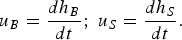
Srebro et al. (Reference Srebro, Elbaz, Sadot, Arazi and Shvarts2003) then extend the BD model by including the amplitude dependence through the parameter E(t) = e −CekhB, where k = 2π/λ is the wavenumber, thereby obtaining the generalized BD model equations:
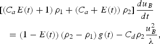
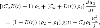
with the coefficient, C e = 3 (2D), 2 (3D).
The BD model described hitherto is valid for single mode perturbations only. For multimode perturbations, Srebro et al. (Reference Srebro, Elbaz, Sadot, Arazi and Shvarts2003) replace λ in the above equations with a characteristic wavelength,  , with the assumption that the BD model governing equations, Eqs. (5)–(6), are applicable with this modified
 . During the early linear growth regime,
 remains constant, but during the late time asymptotic regime,
 grows in a self-similar fashion, i.e., in proportion to the bubble amplitude, h B. Thus,
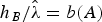 , a function of the Atwood number only. The primary assumption behind the use of the same
 for bubbles and spikes is that they have the same periodicity, which results from the fact that the dominant bubbles inevitably generate the dominant spikes; see Alon et al. (Reference Alon, Hecht, Ofer and Shvarts1995) and Srebro et al. (Reference Srebro, Elbaz, Sadot, Arazi and Shvarts2003) for more discussions. Based on the experiments of Dimonte and Schneider (Reference Dimonte and Schneider2000) and theoretical observations of Oron et al. (Reference Oron, Arazi, Kartoon, Rikanati, Alon and Shvarts2001), Srebro et al. (Reference Srebro, Elbaz, Sadot, Arazi and Shvarts2003) use the following values for b(A):

The characteristic wavelength for multimode perturbations grow as (Srebro et al., Reference Srebro, Elbaz, Sadot, Arazi and Shvarts2003):
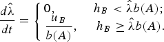
Under this assumption,  starts to increase through bubble competition, i.e., coalescence/merging of contiguous bubbles, only after the bubble amplitude h B has reached the value
 . This equation is solved in addition to Eqs. (5) and (6) for the multimode perturbation cases.
In summary, the generalized BD model described here is suitable for the study of both RT and RM, by using an appropriate acceleration g(t) profile. For RT, g(t) can remain constant such as for instance in a gravitational field, or can change in time if the interface is driven by a blast wave (Balakrishnan & Menon, Reference Balakrishnan and Menon2010; Miles, Reference Miles2009). For RM, on the other hand, g(t) is impulsive and therefore starts from a non-zero value, but rapidly decays to zero. In order to obtain profiles for g(t) that will be inputs to the BD model, it is required to solve the 1D Euler equations; since this study focuses on RT and RM in dusty gases, the multiphase Euler equations are considered and are now elaborated.
2.2. Numerical methodology
To solve the 1D multiphase Euler equations, the formulation presented by Miura and Glass (Reference Miura and Glass1982) is used in this study. In this formulation, the gas is assumed to behave perfect, and viscosity and heat conductivity are neglected except for the computation of the interaction terms. The particles are assumed to be perfectly spherical of uniform size, and are assumed to obey continuum laws; the volume fraction of the particles are neglected. Stated in these terms, the 1D multiphase Euler equations for the continuity, momentum and energy equations for both phases are:
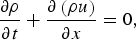
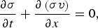

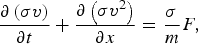

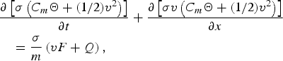
where (ρ, u, T, C v) and (σ, v, Θ, C m) are the (density, velocity, temperature, specific heat) of the gas and dust, respectively, and p is the gas pressure. The terms that appear on the right-hand side of the above equations are the inter-phase interaction terms; here, m is the dust/particle mass, obtained as 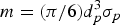 , where d p is the particle diameter, and σp material density of the dust particles. F is the drag force acting on a particle and Q is the heat transfer rate between the two phases, and these terms are computed as follows:


where κ is the thermal conductivity of the gas; C D and Nu denote, respectively, the drag coefficient and Nusselt number, and are computed as:


where Re is the Reynolds number computed as Re = ρ|u − v|d p/μ, Pr is the Prandtl number which is assumed to be 0.7, and μ is the viscosity of the gas assumed to be 1.5 × 10⁻⁵ Kg/ms. κ is computed as κ = μ Cp/Pr, where C p is the specific heat of the gas at constant pressure, obtained as C p = C v + R, where R is the gas constant. Thermodynamic closure is obtained from the perfect gas equation of state:

To solve the above governing equations, we use the MUSCL scheme (Monotone Upstream-centered Schemes for Conservation Laws) (van Leer, Reference van Leer1979) with a flattening procedure to reduce post-shock oscillations (Colella & Woodward, Reference Colella and Woodward1984). The gas fluxes are computed using the HLLC Riemann solver (Toro, Reference Toro1999) and the dust/particle fluxes are evaluated using the Rusanov flux scheme (Rusanov, Reference Rusanov1961). Furthermore, a predictor-corrector scheme is used for time integration. Overall, the scheme is second order accurate in time and space. To validate the 1D two-phase methodology, many canonical tests have been performed, and one such study is presented in the Appendix.
The 1D numerical methodology presented here is used to determine the initial conditions for the BD and MBD models used in the study of RM. The RM studies considered in this paper correspond to a shock-tube configuration, and a grid resolution of 1000 is considered to resolve a 1 m long domain. Analysis shows that with 5000 grid points used to resolve a 1 m long domain, the parameters of interest are insensitive with their corresponding values predicted with the 1000 grid. Thus, 1000 grid points are used for resolving a 1 m long domain. One can also employ high order accurate methods like the spectral volume (Kannan & Wang, Reference Kannan and Wang2009, Reference Kannan and Wang2010) and the spectral difference (Liang et al., Reference Liang, Kannan and Wang2009) methods, since they (1) utilize a spatially high order representation to resolve the physics in a better fashion, (2) can deliver very accurate solutions with smaller degrees of freedom. It is worth mentioning that Kannan was able to obtain extremely accurate solutions with substantially lesser degrees of freedom for a variety of problems (Kannan & Wang, Reference Kannan and Wang2009, Reference Kannan and Wang2010). However, since the crux of the current article is not on the above, we will limit our approach to using classical second order solvers and will consider the above mentioned high order methods in the future. The choice of boundary conditions are not of relevance in this analysis, since the 1D code is used only to determine the immediate post-shock parameters that are inputs to the BD and MBD models for RM analysis, after which the model predicts subsequent growth trends. Having summarized the BD model and the 1D code methodology, we now focus on developing the MBD model.
3. THE MULTIPHASE BUOYANCY-DRAG MODEL
The BD model of Srebro et al. (Reference Srebro, Elbaz, Sadot, Arazi and Shvarts2003) is now extended to account for multiphase effects, and is appropriately referred to as the MBD model. The basic formulation stems from the dusty gas investigations of Saffman (Reference Saffman1962), Michael (Reference Michael1964), and Ukai et al. (Reference Ukai, Balakrishnan and Menon2010). Saffman applied the formulation to laminar flow by deriving the multiphase Orr-Sommerfeld equation; Michael extended this work to the study of plane Poisuelle flow of dusty gases; and Ukai et al. applied the formulation to two kinds of dusty gas Richtmyer-Meshkov instabilities. Here, the effect of dust is described by two parameters—the dust concentration (or number density, N) and a relaxation time (essentially Stokes number, St). The basic assumptions involved in the current formulation are summarized as follows:
1. the dust particles are spherical in shape and are of a uniform size;
2. the bulk concentration of the dust particles, i.e., the dust volume fraction, is negligible;
3. sedimentation effects are assumed to not occur and so the gas-particle mixture stays as a mixture at all times;
4. the gas-particle mixture is assumed to be incompressible for the analysis, as also done so by Saffman (Reference Saffman1962) and Ukai et al. (Reference Ukai, Balakrishnan and Menon2010);
5. the vortex rings around the RT and RM hydrodynamic structures are assumed to not cluster the particles (see Balakrishnan & Menon, Reference Balakrishnan and Menon2010; Balakrishnan et al., Reference Balakrishnan, Ukai and Menon2011 for more discussions on clustering);
6. the dust particles move along the gas streamlines, and so the mean velocities of the dust and the local gas are identical;
7. the number density of the particles is constant everywhere before the disturbance starts to evolve;
8. the dust particles do not cause additional perturbations in the gas, but rather only modify the waves which already exist in the gas (see Saffman, Reference Saffman1962 for more discussions on this).
Stated in these terms, we extend on Srebro et al.'s (2003) work to formulate the MBD model, also deriving ingredients from Ukai et al. (Reference Ukai, Balakrishnan and Menon2010). Recalling the formulation of Saffman (Reference Saffman1962) and Ukai et al. (Reference Ukai, Balakrishnan and Menon2010), small perturnations are considered for the flow variables and the governing equations are linearized; these equations are not summarized here for brevity. The above references then apply boundary conditions at the far-field and at the species interface, following which the first order general expression applicable for RT as well as RM involving dusty gases is obtained as (see Ukai et al., Reference Ukai, Balakrishnan and Menon2010 for a detailed derivation):

where f 1 and f 2 denote, respectively, the particle mass loading in the light and heavy gases and are evaluated as f 1 = mN o/ρ1 and f 2 = mN o/ρ2, where m is the dust particle mass, and N o is the initial dust concentration in number per unit volume. The other terms in Eq. (20) represent the acceleration g(t), wavenumber k (= 2π/λ), wave speed c, particle relaxation time scale τ (subscripts 1 and 2 correspond to fluids 1 and 2, respectively), and i is the complex number √(−1). The relaxation times are obtained as τ1 = τ2 = m/(6π r pμ); note that we have assumed τ1 = τ2, which need not necessarily be always true; the other assumption made is that Stokes drag is valid, as also done so in Saffman (Reference Saffman1962) and Ukai et al. (Reference Ukai, Balakrishnan and Menon2010). Following this, we generalize the formulation of Ukai et al. (Reference Ukai, Balakrishnan and Menon2010) in which the small |kτc| limit was assumed. This formulation can be generalized with the use of the particle Stokes number, St, obtained as St = −ikτc (see the derivation in Ukai et al., Reference Ukai, Balakrishnan and Menon2010 for RM). Thus, Eq. (20) can also be written as:

where St 1 = St 2 is assumed in this study. Furthermore, Ukai et al. (Reference Ukai, Balakrishnan and Menon2010) define a multiphase Atwood number, A m, under the small St (≪1) limit as:

which, for a generic St, can be written as:

Thus, the multiphase effect in the formulation leads to the extension of the classical Atwood number, A, to the multiphase Atwood number, A m, as defined above in Eq. (23). We note that essentially ρ is replaced by  in the multiphase formulation. When τ1 and τ2, or equivalently, St 1 and St 2≪ 1, the multiphase replacement for ρ simply becomes ρ(1 + f); on the other hand, when the particle number density, N, is small, f → 0, resulting in A m → A. Furthermore, when St is very large, the multiphase correction for ρ will be simplify to ρ(1 + f/St). These limiting cases conform to Michael's (1964) results. We use the definition of A m as presented in Eq. (23) to formulate the MBD model, noting that ρ can be replaced by ρ[1 + f/(1+St)], with subscripts 1 and 2 used as appropriate.
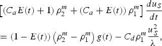
The total mass per unit volume of a bubble enhanced by the particles with number density N o present in it is ρ1 + mN o = ρ1(1 + f 1); similarly, the spike mass per unit volume augmented by particles with number density N o present within it can be expressed as ρ2(1 + f 2). However, since the particles have a delay in response due to finite relaxation time scales (i.e., St ≠ 0), only a fraction of the total particle mass can be used to drive the bubble or spike. We choose this factor as (1 + St) in order to be consistent with Eq. (23). Thus, the effective multiphase bubble and spike masses per unit volume are  and
 , respectively. Following Srebro et al. (Reference Srebro, Elbaz, Sadot, Arazi and Shvarts2003) by considering the added mass term, buoyancy, and drag effects, we can analogously and intuitively obtain the following two equations for the bubble and spike motion in dusty gases:


where, as before, u B and u S denote, respectively, the velocities of the bubbles and spikes, g(t) is the time varying interface acceleration, and λ is the wavelength. We assume that C a and C d remain unaffected by the presence of the particles and use the same values as before. As done in Srebro et al. (Reference Srebro, Elbaz, Sadot, Arazi and Shvarts2003), we then extend the formulation to include amplitude dependence through the parameter 
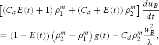
with the coefficient C e remaining the same as before.
For multimode perturbations, we extend Eq. (8) by also accounting for multiphase effects through the b(A m) parameter, defined as:

and also appropriately modify the characteristic wavelength for multimode perturbations to account for multiphase effects:
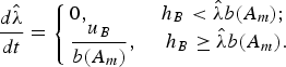
Here, we are using the same definitions for  , with the only replacement for A by A m. Thus, for the MBD model, we solve Eqs. (26) and (27) and, in addition, we solve Eq. (29) for multimode cases. Furthermore, the definition b(A m) is used in place of b(A).
During the early linear perturbation growth, kh B is small, but increases to larger values thereafter as the perturbation switches to the asymptotic stage. Even though the equations derived above for both BD as well as MBD models are non-linear, the early-time linear regime can also be captured. This is because in the linear stage, expanding Eqs. (26–27) to first order in kh B, the perturbation evolution equations for bubbles and spikes take the form:
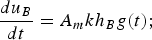
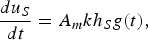
which is consistent with theoretical behavior since the equations are equivalent to ḧ(t) = A mkg(t)h(t). During the early linear growth,  is not changed with time, but the growth is self-similar in the asymptotic stage. A similar reasoning was used by Srebro et al. (Reference Srebro, Elbaz, Sadot, Arazi and Shvarts2003) to demonstrate the validity of the baseline BD model for both linear as well as the asymptotic stages of evolution. Thus, the non-linear Buoyancy-Drag theory is also applicable for the early linear stages with the small kh B and constant
 approximations.
In summary, the generalized MBD model described here is suitable for the study of both RT and RM in dusty gases. For RT, the MBD model can be directly applied to evaluate bubble and spike growth. For RM, on the other hand, knowledge of g(t) as well as the post-shock ρ1, ρ2, N 1, and N 2 are also required, which are evaluated from the 1D simulations described in Section 2.2. Here, N 1, and N 2 denote, respectively, the post-shock particle number densities in the fluids 1 and 2. In the following sections, the baseline BD model of Srebro et al. (Reference Srebro, Elbaz, Sadot, Arazi and Shvarts2003) is verified for both RT and RM involving both single and multi-mode perturbations, following which the MBD model is tested.
4. RESULTS AND DISCUSSION
4.1. Verification of the Srebro et al. (Reference Srebro, Elbaz, Sadot, Arazi and Shvarts2003) BD model
First, we verify the efficacy of the baseline BD model as developed by Srebro et al. (Reference Srebro, Elbaz, Sadot, Arazi and Shvarts2003) for RT and RM applications. To this end, we focus on single-mode RT (SMRT), multi-mode RT (MMRT), single-mode RM (SMRM), and multi-mode RM (MMRM). It is customary to ensure that the choice of the time step, Δt, is sufficiently small so that the BD model simulation results are meaningful. For RT, we ensure that Δt ≪ τRT, and for RM, Δt ≪ τRM, where τRT and τRM denote, respectively, the time scales for RT and RM, given by  (Ramshaw, Reference Ramshaw1998) and
 (Ukai et al., Reference Ukai, Balakrishnan and Menon2010), where Δv is the velocity of the interface after the shock passage.
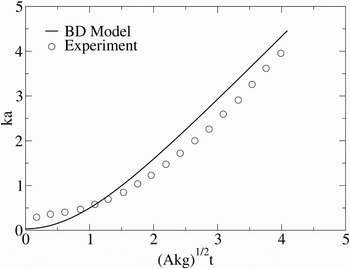
For SMRT, we consider the experimental results of Wilkinson and Jacobs (Reference Wilkinson and Jacobs2007), which correspond to A ~ 0.15. In their experiment, the initial amplitude, a o was in the range 0.248–2.718 mm; we assume a o = 0.25 mm for the BD model analysis as the exact value from the experiment is not known. Figure 1 shows the non-dimensional amplitude (ka, k = 2π/λ) versus non-dimensional time for a constant acceleration, g. As evident, the BD model reasonably predicts the overall growth trends although slight deviations are observed at later times, (Akg)1/2t ~ 3.5. These discrepancies may result from differences in the choice of the initial amplitude used in the experiments and the current BD model, or presumably from acceleration on the fluid not being exactly constant (in the experiment of Wilkinson and Jacobs (Reference Wilkinson and Jacobs2007), an average measured acceleration was used). The growth trend of ka conforms to an exponential variation with t until ka ~ 1, after which transitions to a linear variation with t, in agreement with theory (Goncharov, Reference Goncharov2002). Thus, the overall growth trends of the amplitude are in reasonable agreement both with experiments as well as theory, thereby exemplifying the efficacy of the BD model to predict SMRT.
Single-mode RT. Experimental results are from Wilkinson and Jacobs (Reference Wilkinson and Jacobs2007).

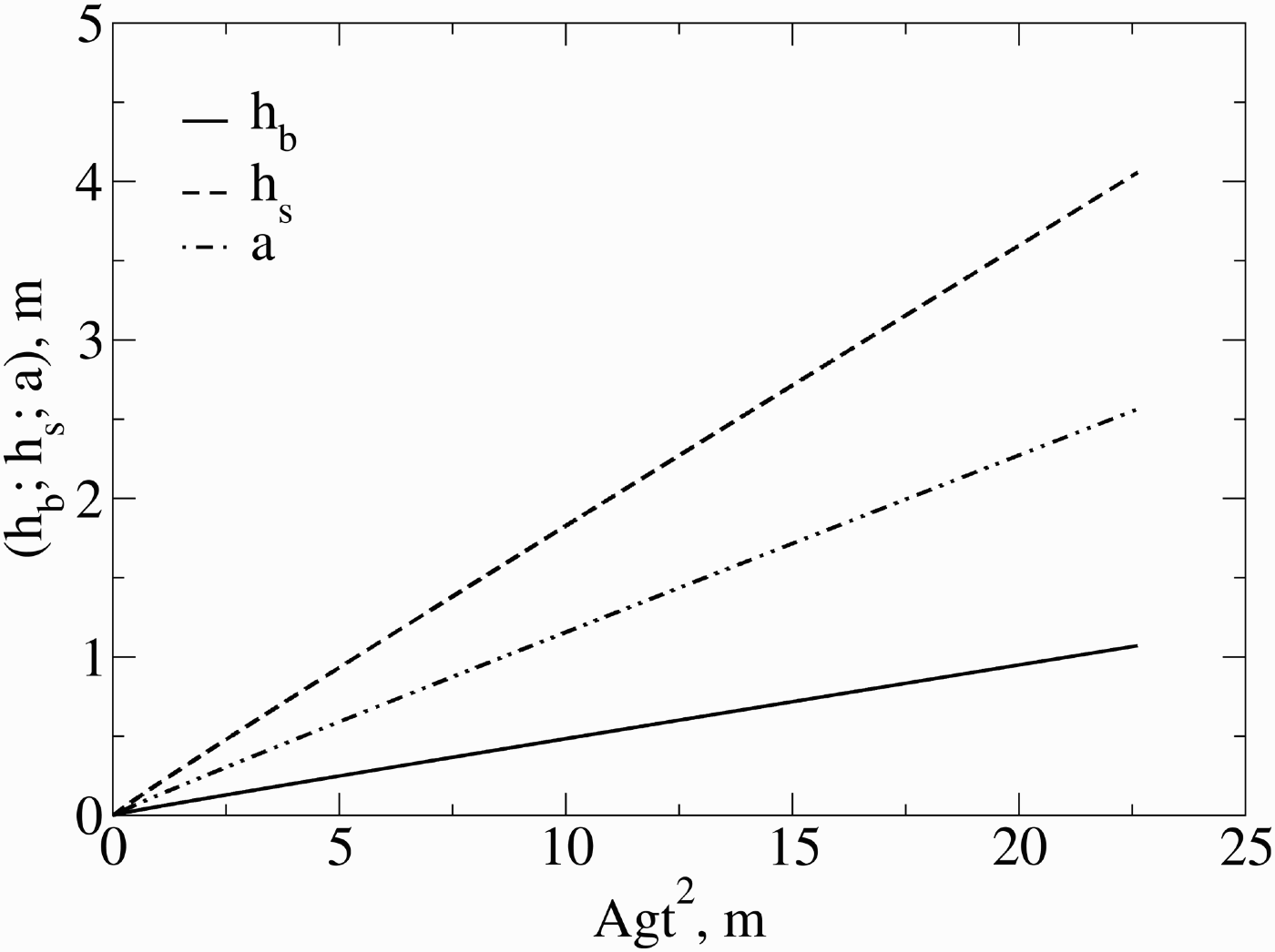
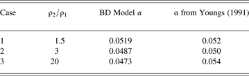
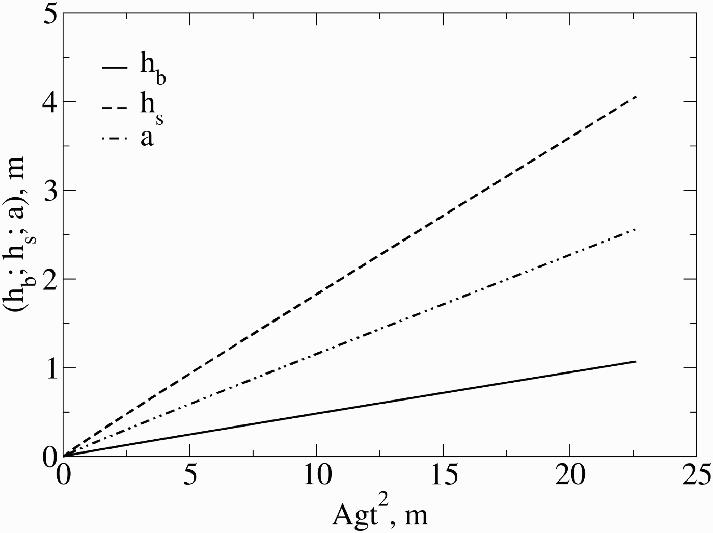
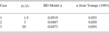
Next, we apply the baseline BD model to investigate MMRT, focusing on the simulation results of Youngs (Reference Youngs1991), where three different density ratios, ρ2/ρ1 = 1.5, 3 and 20 were considered. For the BD model, we use  and h b = h s = 0.1 mm as initialization, so that the initial ka = 0.06 ≪ 1, resulting in linear growth rates. Figure 2 shows the bubble height (h b), spike height (h s), and amplitude (a) versus Agt 2; as evident, the heights and the amplitude vary linearly with Agt 2, a well established classical result for MMRT. The slope, α, of the bubble height, h b, is computed for the three chosen ρ2/ρ1 values, and are summarized in Table 1, along with the corresponding slopes obtained in the simulations carried out by Youngs (Reference Youngs1991). As evident, α ≈ 0.05, a classical RT result; even the BD model α predictions are in reasonable agreement with Youngs (Reference Youngs1991), with the deviations widening for higher ρ2/ρ1 ratios. From this result, we believe that the BD model is better suited for lower density ratios (and lower A); as A→ 1, some modifications may be required, and will have to be addressed in the future. This study verfiies the baseline BD model for MMRT.
Multi-mode RT: h b, h s and a versus Agt 2 for ρ2/ρ1 = 20.
MMRT slopes, α, predicted by the current BD model and as obtained by Youngs (Reference Youngs1991)
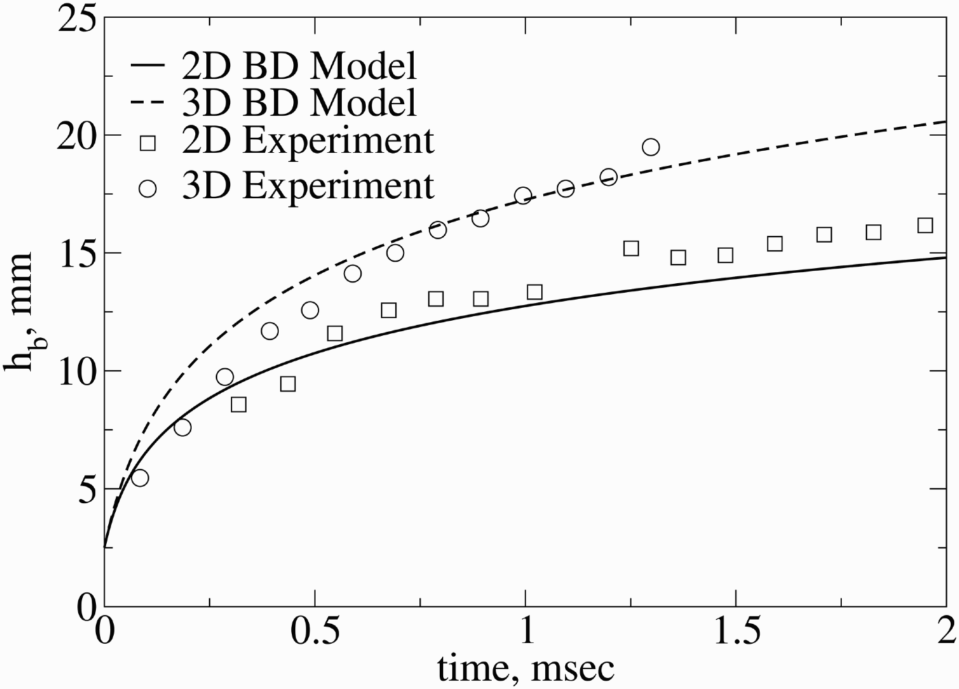
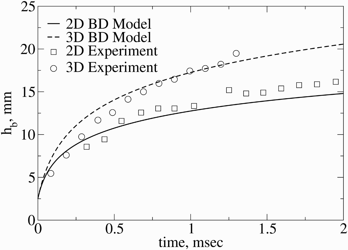
We next focus on SMRM; in particular, we are interested in the experiments of Erez et al. (Reference Erez, Sadot, Oron, Erez, Levin, Shvarts and Ben-Dor2000) and the analysis done by the same research group in Shvarts et al. (Reference Shvarts, Sadot, Oron, Kishony, Srebro, Rikanati, Kartoon, Yedvab, Elbaz, Yosef-Hai, Alon, Levin, Sarid, Arazi and Ben-Dor2000). Here, RM experiments involving both 2D and 3D perturbations in air/SF 6 combinations are considered, with an incident shock Mach number of 1.25 and an initial λ =26 mm. The 1D code described in Section 2.2 is used to estimate the initial interface velocity, ΔV, that is used as an input to the BD model, i.e., the initial velocity of the interface after the passage of the incident shock. Figure 3 presents the BD model results along with experimental results of Erez et al. (Reference Erez, Sadot, Oron, Erez, Levin, Shvarts and Ben-Dor2000) and Shvarts et al. (Reference Shvarts, Sadot, Oron, Kishony, Srebro, Rikanati, Kartoon, Yedvab, Elbaz, Yosef-Hai, Alon, Levin, Sarid, Arazi and Ben-Dor2000); we apply the 2D and 3D versions of the BD model as appropriate. As evident, the BD model predictions are in reasonable agreement with the experiments, thereby verifying the application of the baseline BD model for SMRM. h b for the 3D initial perturbation is about 25% greater vis-à-vis the 2D initial perturbation, due to the smaller drag coefficient for 3D (Alon et al., Reference Alon, Hecht, Ofer and Shvarts1995).
Single-mode RM: h b for 2D and 3D initial perturbations. Experimental results are from Erez et al. (Reference Erez, Sadot, Oron, Erez, Levin, Shvarts and Ben-Dor2000) and Shvarts et al. (Reference Shvarts, Sadot, Oron, Kishony, Srebro, Rikanati, Kartoon, Yedvab, Elbaz, Yosef-Hai, Alon, Levin, Sarid, Arazi and Ben-Dor2000).
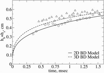
Finally, we verify the baseline BD model for the study of MMRM, focusing on the air/SF 6 experiments of Erez et al. (Reference Erez, Sadot, Oron, Erez, Levin, Shvarts and Ben-Dor2000), as also done in Srebro et al. (Reference Srebro, Elbaz, Sadot, Arazi and Shvarts2003). Due to the lack of exact information on the nature of the initial perturbation, the initial choice of  and h = h b + h s are varied to match with the experiments along with the assumption h b = h s initially (a similar approach was undertaken by Srebro et al., Reference Srebro, Elbaz, Sadot, Arazi and Shvarts2003). Figure 4 presents the total mixing zone width, h, versus time using both the 2D and 3D versions of the baseline BD model; two sets of experiments from Erez et al. (Reference Erez, Sadot, Oron, Erez, Levin, Shvarts and Ben-Dor2000) and Srebro et al. (Reference Srebro, Elbaz, Sadot, Arazi and Shvarts2003) are presented. Analysis shows that
 and h = 0.07 cm results in reasonable agreement with the experimental data. Although the origianl experiments of Erez et al. (Reference Erez, Sadot, Oron, Erez, Levin, Shvarts and Ben-Dor2000) involved both incident and re-shocks, we, however, focus only on the incident shock in this study, and therefore terminate the BD model simulation just before the arrival of the reshock. In the future, the BD model for re-shocked systems needs to be revisited so as to ascertain the model's prediction of the expected phase reversal growth trends. We curve-fit the bubble height h b, spike height h s, and amplitude
 as power laws with time, i.e., h b ~ t θb, h s ~ t θs, a ~ t θa. With the 3D version, we obtain θb = 0.164, θs = 0.297, and θa = 0.262; the corresponding values with the 2D version are θb = 0.222, θs = 0.327, and θa = 0.294. These values compare reasonably well with Srebro et al. (Reference Srebro, Elbaz, Sadot, Arazi and Shvarts2003), who state that the experimental θa = 0.24 and their numerical θa = 0.29 and 0.32, respectively, with the 3D and 2D models, for the same initial conditions. This study exemplifies the applicability of the baseline BD model for MMRM.
Multi-mode RM: h b +h sversus time. Experimental results are from Erez et al. (Reference Erez, Sadot, Oron, Erez, Levin, Shvarts and Ben-Dor2000); Srebro et al. (Reference Srebro, Elbaz, Sadot, Arazi and Shvarts2003).

In summary, we have verified the ability of the baseline BD model to predict the growth trends encountered in SMRT, MMRT, SMRM, and MMRM. The focus now is to test the MBD model for similar cases and to understand the underlying physics. Of particular interest is to investigate the effect of particle loading, N, and particle radius, r p, on the amplitude growth trends. To this end, the next section focuses on applying the MBD for the study of similar problems in dusty gases. It is emphasized that to the best of the authors' knowledge, no experimental results exist for RT and RM growth in dusty gases; thus, we are unable to compare MBD model predictions with any dusty gas experiments.
4.2. Dusty Gas RT Using the MBD Model
The role played by solid particles in the mixing layer growth in RT is investigated, first for SMRT, and then for MMRT. It is of interest to study the effects of particle loading, N, and particle size, r p. We apply the MBD model for cases corresponding to A = 0.5, ρ1 =1 Kg/m3, g = 1 m/s2, initial wavelength, λ0 =1 cm (λ for SMRT;  for MMRT) and initial amplitude, a 0 = 0.1 mm. For MMRT, the ratio,
 as defined in Eq. (28) is used.
4.2.1 SMRT
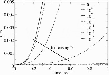
We apply the MBD model for the above chosen parameters; first, we investigate the effect of N on the amplitude growth. r p = 40 μm is considered, and this corresponds to St ~ 1. We consider a baseline particle-free (N = 0 m−3) case in addition to N in the range 108—1013 m−3. Figure 5 shows the amplitude, a, versus time. As expected, a grows slower for higher N, since particles serve as an obstruction to the bubble and spike motion. For N = 108 m−3, the amplitude growth tends to the particle-free growth as too few particles are present to offer resistance to the growth of the mixing layer. This trend is expected, since only f depends on N and r p is independent; therefore, the term 1 + f/(1 + St) → 1 as N → 0. On the other hand, as N increases, 1 + f/(1 + St) → f/(1 + St). We also compute the late time slopes of the bubble and spike amplitudes to obtain the respective late time constant bubble and spike terminal velocities (U RT(B/S)). The MBD model predictions for U RT(B/S) are in accordance with the value obtained by equating the buoyancy and drag terms:

Multiphase single-mode RT: amplitude versus time for different particle loading with r p = 40 μm. The legend denotes the value of N in number per m3.

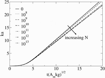
consistent with the results obtained by Oron et al. (Reference Oron, Arazi, Kartoon, Rikanati, Alon and Shvarts2001), albeit with A m in place of A (the + sign corresponds to the bubbles and the − sign for the spikes). It is also of interest to consider the trends in the growth of the non-dimensional amplitude (ka) versus non-dimensional time (t(A mkg)1/2), and is plotted in Figure 6. It is interesting to note that as N increases, the non-dimensional profiles also tend to converge, thereby creating a band of solutions between A m → A and A m → 0. The study is repeated for a different choice of r p and similar ka trends are observed, albeit for a different range of N; this is because in the term f/(1 + St), f ~ r p3 and St ~ r p2, and so for a different r p, f/(1 + St) will follow a different trend for a given N. However, the results are observed to still be contained within the same band, i.e., A m → A (upper limit) and A m → 0 (lower limit); these results for different r p are not presented here for brevity. Thus, a band of solutions is identified for the growth of the non-dimensional amplitude versus non-dimensional time, for dusty gas SMRT.
Multiphase single-mode RT: non-dimensional amplitude versus non-dimensional time for different particle loading with r p = 40 μm. The legend denotes the value of N in number per m3. The result corresponding to N = 108 m−3 is coincident with N = 0 m−3 and so is not clearly visible.

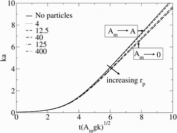
Next, we investigate the effect of r p for a fixed N = 1010 m−3. We consider particle sizes in the range r p = 4–400 μm, corresponding to different St. Here, r p = 4 μm corresponds to St ~ 0.01, r p = 40 μm to St ~ 1, and r p = 400 μm to St ~ 100. Figure 7 shows the non-dimensional amplitude versus non-dimnesional time. Again, as evident, the results are contained within the bands corresponding to A m → A and A m → 0. For very small r p, too little particle mass is present to influence bubble and spike motion, and so the results conform to the particle-free case (A m = A), the upper limit. Note that for very small r p, 1 + f/(1 + St) → 1. On the other hand, when very large particle sizes are considered, 1 + f/(1 + St) → 6πr pμN/ρ. Thus, for too large an r p, ρ[1 + f/(1 + St)] → 6π r pμ N, i.e., independent of ρ. Hence, the initial density ratio loses significance and the mixing layer evolves tending to the A m → 0 limit (lower limit) for large particle sizes. Even the bubble and spike steady-state velocities at late times are observed to conform to Eq. (31). This study demonstrates that a band of solutions is observed also for the MMRT in dusty gases, and that the choice of A m for dusty gases can be physically analogous to A for pure (dust-free) gases.
Multiphase single-mode RT: non-dimensional amplitude versus non-dimensional time for different particle sizes with N = 1010 m−3. The legend denotes the value of r p in μm.

4.2.2. MMRT
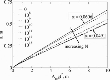
To investigate multiphase MMRT, as noted in Eq. (28), we use b(A m). The same initial conditions are used for this study, with the difference being the use of  instead of λ, and the corresponding equation for the wavelength growth rate (Eq. (29)). Figure 8 displays the growth of amplitude, a, versus A mgt2, for a fixed r p = 40 μm (this corresponds to Stokes number, St ~ 1), for a range of N. As evident, higher N results in subdued mixing layer amplitude growth as more particles obstruct the rise of bubbles and the fall of spikes. The linear trend between a and A mgt2 suggests that the well established a ~ t 2 result also holds for multiphase systems with the use of A m in place of A. Again, the results are contained within a band, with the upper limit corresponding to A m → A (for N → 0) and the lower limit to A m → 0 (for N → ∞). The slopes of these curves, α, are evaluated to be α = 0.0606 for the upper limit and α = 0.0491 for the lower limit. Interestingly, these values are similar to the classical result of α ~ 0.05 reported by Youngs (Reference Youngs1984, Reference Youngs1989, Reference Youngs1991, Reference Youngs1994). Thus, it is possible that some of the established theories on hydrodynamic instability growth can be extended to multiphase systems as well by replacing A with A m.
Multiphase multi-mode RT: amplitude versus A mgt2 for different particle loading with r p = 40 μm. The legend denotes the value of N in number per m3.

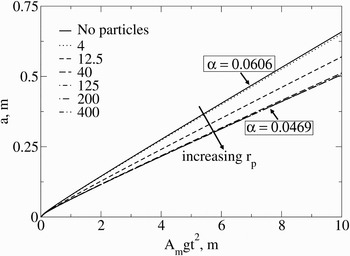
Next, we fix the particle loading at N = 1011 m−3 and vary particle sizes in the range r p = 4–400 μm, for the same a o, initial  , A, ρ1, and g. Here, r p = 4 μm corresponds to St ~ 0.01, r p = 40 μm to St ~ 1, and r p = 400 μm to St ~ 100. Figure 9 shows the amplitude variation versus A mgt2 and, as evident, linear trends (in t 2) are observed at later times, with the amplitudes contained within a band. For very small particle sizes, the total particle mass is negligible to have an effect on the bubble and spike growth and so the result converges to the particle-free case; for very large particle sizes, on the other hand, the results again converge to the A m → 0 solution as before. The slopes of the band boundaries are determined to be α = 0.0606 for the upper limit (A m → A) and as α = 0.0469 for the lower limit (A m → 0). Such banded solutions indicate that the slope, α, increases with A m for a given A.
Multiphase multi-mode RT: amplitude versus A mgt2 for different particle sizes with N = 1011 m−3. The legend denotes the value of r p in μm.

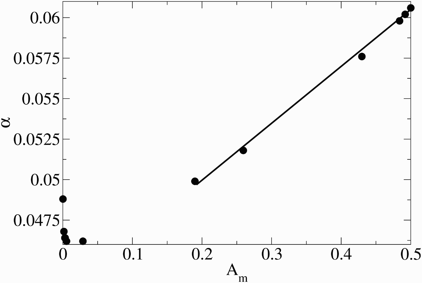
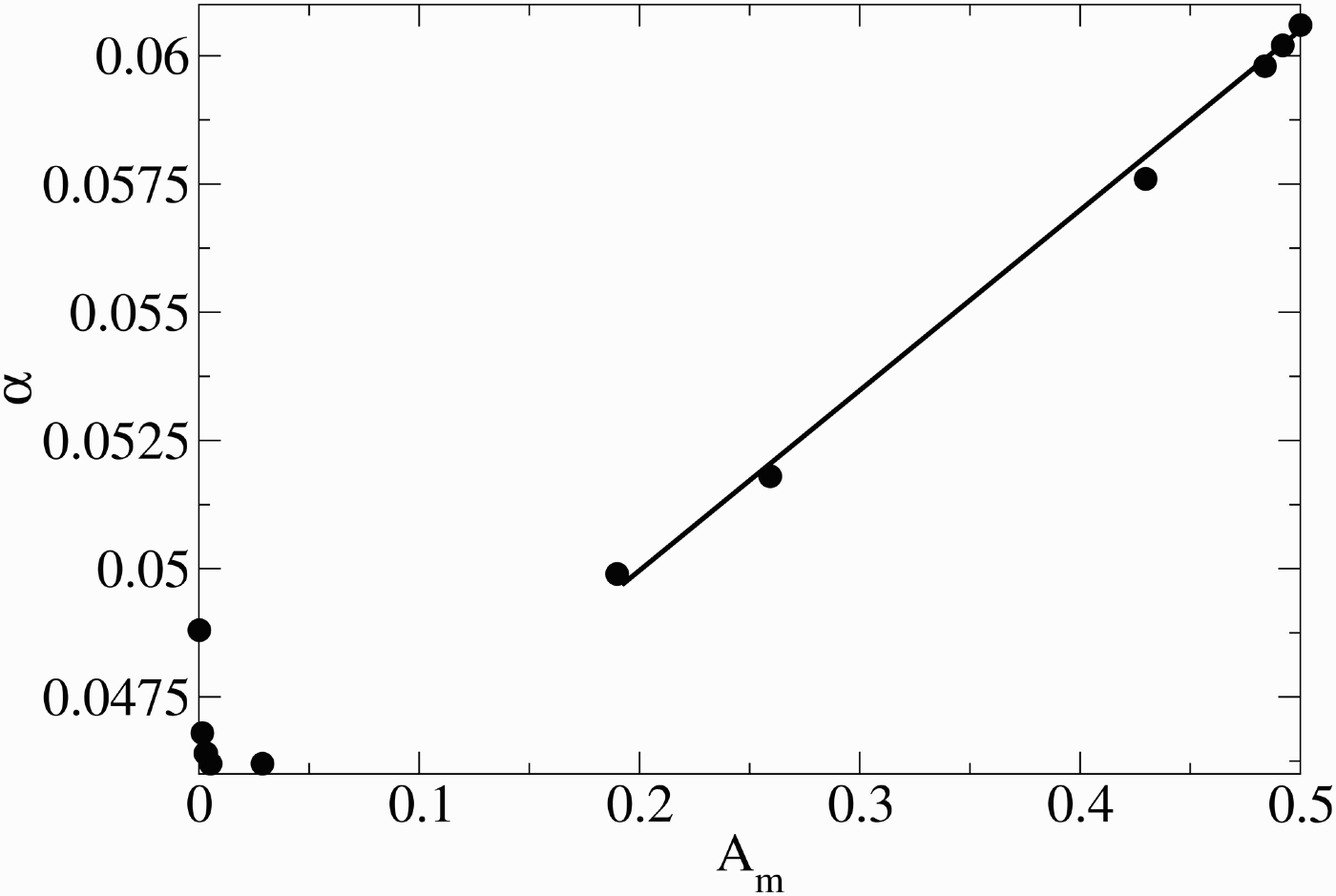
It is also of interest to consider the trends in the slope of the amplitude versus A mgt 2 curves for the different 3D cases considered for the multiphase MMRT analysis, for this directly indicates dependence of the t 2 law for different particle sizes and loadings. Figure 10 shows α = a/(A mgt 2) versus A m for these different MMRT cases considered; it is observed that for A m> 0.2, a linear trend is observed. Note that these results correspond to a fixed A = 0.5. In the future, we will be investigating the α trend versus A m for different choices of A. In Figure 10, for very small A m, however, a scatter is observed in the α predictions, due to which we believe that the MBD model may not be well suited for A m → 0. This is because when the total particle mass is large (as is for A m → 0 cases), some of the assumptions that were stated earlier in the formulation (Section 3) can fail. For instance, the assumption that the particle-gas mixture remains uniform at all times is of concern under high particle mass cases. Furthermore, when A m → 0, since the particle mass outweighs the gas mass, the treatment of the dusty gas mixture as a fluid presumably fails. Due to these effects, the MBD model needs further improvement for A m → 0 cases.
Variation of α with A m for different cases considered in MMRT. A = 0.5 for all these cases.
4.3. Dusty gas RM using the MBD model
4.3.1. SMRM
Here, we extend on the 3D cases considered earlier for the single phase RM, and investigate the bubble and spike growth when particles are present. In both the BD and MBD models, the acceleration profile can be crucial in deciding whether RM can be assumed to be an impulsive case of RT. For instance, it has been demonstrated by Wouchuk (Reference Wouchuk2001) that RM involving weak shocks behave as an impulsive case of RT, with impulsive predictions showing deviations even for Mach 1.5 shocks. For very strong shocks, models that treat RM as an impulsive RT case need to be revisited in the future, with perhaps the use of a g(t) profile varying over a finite albeit small time interval. Such profiles may be essential for strong shock RM in order to more accurately predict the perturbation growth rates; studies to this end will be considered in the future. In the present investigation, only relatively weak shock (Mach number < 1.5) RM cases are considered.
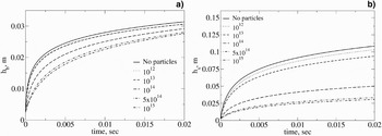
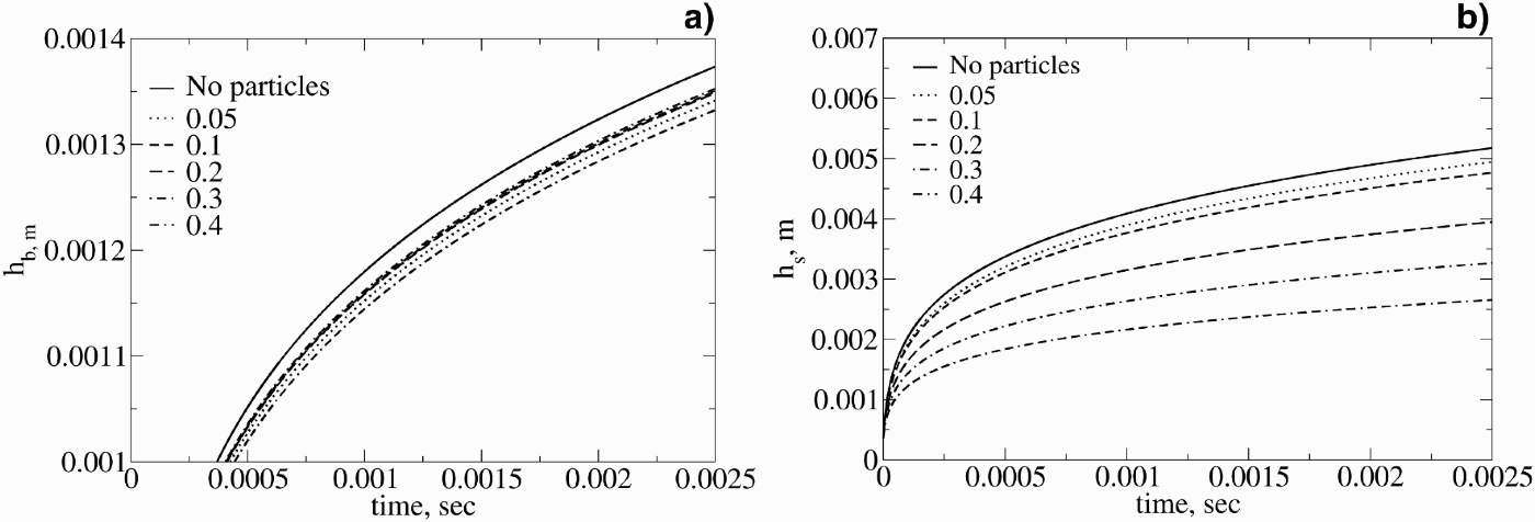
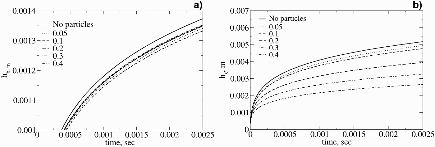
The choice of r p or N used in these cases will be different from those considered for RT due to different time scales involved for RT and RM. Thus, comparing the results between RM with RT for the same r p or N does not correspond to any physical significance; the range of r p and N of interest to the analysis is thus different between RT and RM for the same reason. Figure 11 shows the (a) h b and (b) h s growth with time for a fixed r p = 1.5 μm for different values of N. As evident, both h b and h s show subdued growth with time as the number of particles increases. Whereas the bubble height is only affected by ~ 20% for the particle number density range considered, the spike heights show more pronounced variations, with h s being only one-fourth for the denser cases considered vis-à-vis the particle-free case. This study illustrates that the spike growth shows higher sensitivity to the presence of particles than the bubbles, presumably due to the higher inertia involved for the spikes. Next, we investigate the effect of r p for a fixed N = 1013 m−3; the bubble and spike heights are presented in Figure 12. Even for these cases, both h b and h s show subdued growth with an increase in r p, with the spikes showing a higher dependence. It is also interesting to note from Figure 12 that whereas the particle-free and small particle cases show a rapid increase in h b and h s at early times followed by slower exponential growth at later times—typical for RM instabilities, for larger particles, on the other hand, the growth trends are more gradual even at early times—similar to RT growth. Essentially, this means that RM with large particle sizes (therefore, slow response times) behave in some physical sense similar to RT. This observation was also made in Ukai et al. (Reference Ukai, Balakrishnan and Menon2010) based on 2D simulations, and is owing to the slow response of the larger particles, due to which the bubble and spike growth does not stay impulsive, but rather switches gradually to a more continuous growth. It is noteworthy of mention that the MBD model is able to predict this particle-size sensitivity on the bubble and spike growth trends at early times.
Multiphase single-mode RM: (a) bubble amplitude and (b) spike amplitude growth with time for a fixed r p = 1.5 μm. The legend denotes different values for N in m−3. In (a), the N = 1012 case is coincident with the “No particles” case and is thus not clearly visible.

Multiphase single-mode RM: (a) bubble amplitude and (b) spike amplitude growth with time for a fixed N = 1013 m−3. The legend denotes different values for r p in μm.

4.3.2. MMRM
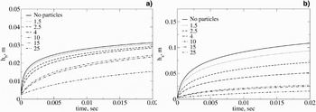
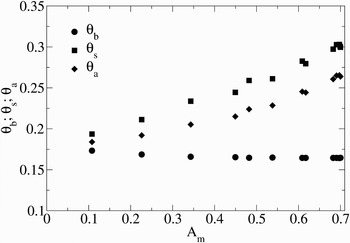
Finally, we shift our focus to the investigation of multiphase MMRM. The effect of r p on the growth of h b and h s are investigated for a fixed N = 1016 m−3 in Figure 13, for a fixed A = 0.7. As before, with the increase in particle size—and therefore particle mass—subdued h b and h s are observed, with the spikes showing a higher sensitivity to the presence of particles. Similar results are observed also for higher N for a fixed r p, not shown here for brevity. Power law growth trends with time are observed for h b, h s, and a for the different 3D multiphase MMRM cases considered, and these are plotted versus A m in Figure 14; here, h b ~ t θ b; h s ~ t θs; a ~ t θa. As observed, θb linearly decreases for low A m from ~ 0.17 to 0.165, and stays nearly constant with A m for A m> 0.5. θs, and θa, on the other hand, are observed to non-linearly increase with A m in the A m = 0.1 to 0.7 range. Similar trends were reported for the single-phase MMRM considered in Oron et al. (2001). Thus, the MBD model can be used to obtain power law dependence for multiphase MMRM. Although only A = 0.7 is considered in this study, in the future such power law coefficients for a wider range of A can be investigated.
Multiphase multi-mode RM: (a) bubble amplitude and (b) spike amplitude growth with time for a fixed N = 1016m−3. The legend denotes different values for r p in μm.
Variation of θ with A m for different 3D cases considered in MMRM. A = 0.7 is fixed.

4.4. Four New Classes of Problems
We have hitherto analysed RT and RM in pure gases using the BD model, and in dusty gas mixtures using the MBD model. This leads to a hybrid scenario wherein a combination of the two studies is possible, i.e., when RT or RM involves pure gases in certain regions, and dusty gases otherwise. Thus, we develop a hybrid BD/MBD model that uses BD in pure (dust-free) regions and MBD in dusty gas regions. Based on the current analysis of multiphase RT and RM, 4 new classes of problems are identified that are tractable to analysis with such a hybrid BD/MBD model. These are summarized as:
1. Bubbles in a pure gas RT or RM rising into a region of particles;
2. Spikes in a pure gas RT or RM falling into a region of particles;
3. Bubbles in a multiphase RT or RM rising into a region of pure gas;
4. Spikes in a multiphase RT or RM falling into a region of pure gas.
Here, bubbles or spikes, corresponding to single- or multi-mode, RT or RM, in a pure gas (or dusty gas) can rise or fall, respectively, into a dusty (pure) gas, as the case may be. Under such scenarios, the BD model must be used for pure gas regions, and the MBD model in dusty regions, thereby leading to a hybrid model. In this sub-section, only the MMRT will be studied for these identified possibilities, as the goal here is to demonstrate the efficacy of the hybrid solver for the study of such kinds of RT and RM, which are, to the best of the author's knowledge, new in the literature. In addition, the physics of these parametric studies are not elaborated, as the goal of the current analysis is to demonstrate the application of the BD/MBD hybrid model and identify four new classes of problems related to dusty gas MMRT. In the future, such possibilities for SMRT, SMRM, and MMRM needs to be revisited.
We consider the same set of initial conditions for  , a o, g, ρ1, ρ2, and A considered in the MMRT analysis from Section 2, with differences in the particle distribution in space. r p = 40 μm is used as it corresponds to St ~ 1, which is of interest here; the particle number density is taken to be N = 1010 m−3. For this analysis, we assume, for bubbles rising or spikes falling into a region of particles, the interface between the pure and dusty gases are located at a height of 1.5 m from the initial pure gas interface that separates the two fluids corresponding to ρ1 and ρ2. For ease of discussion, we refer to the initial interface between the two fluids corresponding to ρ1 and ρ2 (when amplitude, a = a o) simply as “interface,” and the interface between the pure fluids and the dusty gases as “multiphase interface (MI).” Note that for the analysis of bubbles rising into a particle region, the MI lies on the side of the bubbles (side of ρ2). Likewise, for spikes falling into a region of particles, the MI is located on the side of the spikes (side of ρ1). Similar distinction is emphasized for the analysis of bubbles rising or spikes falling from a dusty gas into a region of pure gas—here, the pure gas is identified by the gas that is present on the same side as the bubble rise or spike fall.
4.4.1. Bubbles in a Pure Gas MMRT Rising into a Region of Particles
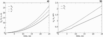
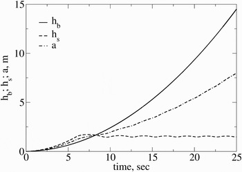
First, we analyze the rise of pure gas bubbles into a region of dusty gas located 1.5 m away from the initial interface. For this analysis, we use the BD model for both bubbles and spikes until h b reaches 1.5 m, after which the MBD model is employed for the bubbles, but the BD model is continued for the spikes, since only the bubbles encounter the dusty gas region. The parameter b(A m) is used as this case involves bubbles encountering both pure fluids as well as dusty gases. Figure 15 shows (a) h b, h s, a and (b) u b, u s, and as evident, the bubble amplitudes do not show noticable differences as they enter into the dusty gas region. From Figure 15(b), u b only shows a minor “kink” around 7.5 s, and quickly adjusts to a linear velocity profile thereafter, resulting in continued h b ~ t 2 growth. The buoyancy term in the MBD model increases in magnitude as ρ2m – ρ1m increases when the bubbles rise into the particle region. This inevitably accelerates the bubble front, albeit only to a small extent in the present case, and causes the kink in the velocity profile. Thus, the dusty gas region has an accelerating influence, albeit small, on the rising bubbles for the case considered.
Bubbles in a pure gas MMRT rising into a region of particles: (a) h b, h s and a; (b) u b and u s.

4.4.2. Spikes in a Pure Gas MMRT Falling Into a Region of Particles
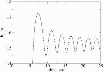
Next, we focus our attention on the fall of spikes into a region of particles, using the same initial conditions noted. MI is now switched to the side of the spike fall; b(A) is used instead of b(A m), since the parameter b is related to bubbles, which rise only into pure gases for the present case. Figure 16 displays h b, h s, and a. It is observed that even though h s > h b at early times as expected, once the spikes enter the dusty gas region (h s > 1.5 m) they slow down and oscillate about the MI (located at 1.5 m), thereby allowing for h b > h s at later times. This oscillation of the spike front is owing to A m becoming negative for the spikes inside the dusty gas, thereby reversing the buoyancy force. For the BD/MBD analysis, the sign of the drag term for the spikes is reversed based on the direction of motion, so that the drag term always opposes its motion. Subsequently, the spikes again enter the pure gas region, after which the buoyancy term once again changes sign, causing the spikes to fall again into the dusty region. Then, the sign of the buoyancy term again changes, and such oscillations are repeated, leading to a gravity wave-like phenomenon. The amplitude of the oscillation for every subsequent penetration decreases in time as the spikes lose momentum to the surrounding dusty gas due to drag. We zoom h s in the vicinity of the MI and present in Figure 17 a closer view of the oscillatory nature of h s. As evident, the local maxima and minima in the spike front decays for every subsequent penetration into the dusty gas due to drag effects. Even the oscillation frequency decreases for every subsequent penetration, as the buoyancy effects decrease for every subsequent penetration, due to which the spikes require lesser time to slow down to rest and thereafter reverse direction. In the future, the dependence of this oscillation frequency on r p and N needs to be revisited.
Spikes in a pure gas MMRT falling into a region of particles.

Oscillatory h s behavior as spikes in a pure gas MMRT fall into a region of particles.

4.4.3. Bubbles in a Multiphase MMRT Rising into a Region of Pure Gas
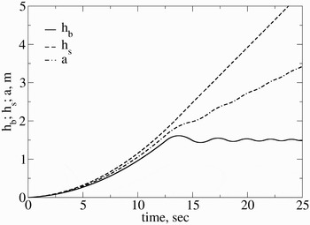
We now investigate the rise of bubbles in a multiphase MMRT into a region of pure gas. Again, the MI is located 1.5 m above the initial interface that separates the two fluids, ρ1 and ρ2. The parameter b(A m) is used since this study involves bubbles encountering dusty gases. Figure 18 shows h b, h s, and a versus time. As before, the bubble height, h b, shows a gravity wave-like phenomenon as the term ρ2m − ρ1m changes sign alternatively, thereby changing the sign of the buoyancy term. For the BD/MBD analysis, the sign of the drag term is changed to ensure that it always opposes the bubble motion. Even for the bubbles considered here, both the oscillation amplitude and frequency decrease with time.
Bubbles in a multiphase MMRT rising into a region of pure gas.

4.4.4. Spikes in a Multiphase MMRT Falling into a Region of Pure Gas
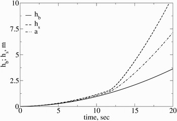
Finally, we investigate spikes in a multiphase MMRT falling into a region of pure gas. The parameter b(A m) is used in the analysis since the bubbles always remain in a dusty gas for this case. Figure 19 shows h b, h s and a versus time. The spike front accelerates as it enters into the pure gas beyond h s> 1.5 m, as ρ2m − ρ1m in the buoyancy term increases in magnitude, hence accelerating the spike front.
Spikes in a multiphase MMRT falling into a region of pure gas.

Overall, these parametric studies have identified four new classes of problems that can be investigated using the currently developed MBD model. Since the goal of this paper is to demonstrate the ability of the MBD model for problems of this kind, the four parametric studies are not studied in elaborate detail. Furthermore, studies along these lines for SMRT, SMRM and MMRM also needs to be investigated in the future. The MBD model offers leverage for such problems.
4.5. Extensions to the MBD Model
Through the course of this paper, we have formulated and applied the MBD model for a wide variety of RT and RM problems and the model is able to accurately predict the bubble and spike growths under different multiphase conditions. However, experiments on multiphase RT and RM are limited in the literature and so the model predictions could not be directly verified with experiments. As shown earlier, the MBD model needs to be revisited for A m → 0, i.e., when the particle mass is much higher than the gas; under this scenario, the treatment of the gas-particle mixture as a pseudo-gas mixture is stretched, and so the model needs revisions for this limiting end. Furthermore, for RM, we have applied the MBD model only for a single shock system, and so the MBD model needs further testing for re-shocked RM which causes phase-reversal (Srebro et al., Reference Srebro, Elbaz, Sadot, Arazi and Shvarts2003; Leinov et al., Reference Leinov, Malamud, Elbaz, Levin, Ben-Dor, Shvarts and Sadot2009). For strong shock RM in dusty gases, the use of a non-impulsive g(t) profile may be warranted in order to more accurately predict growth rates. Such modifications can be investigated in future studies with the MBD model.
Other applications include the study of explosions in multiphase environments (Balakrishnan & Menon, Reference Balakrishnan and Menon2010; Balakrishnan et al., Reference Balakrishnan, Ukai and Menon2011; Balakrishnan, Reference Balakrishnan2010), for which the MBD model needs to be extended to account for geometrical divergence effects. For this, the decompression term introduced in Miles (Reference Miles2009) for the single-phase BD model can be used in the MBD model. Other physical problems of interest include the application of the MBD model to reactive systems, where the Stokes number can change with time for burning particles, which can also result in interesting results; in addition, heat release effects associated with burning particles can also drive the bubble and spike growth due to volumetric expansion, and these problems can also be investigated with the MBD model with some minor corrections incorporated. Furthermore, for blast wave driven systems, a time-varying acceleration profile can be considered and the MBD model can be applied under such conditions as well to investigate blast driven RT and RM in dusty gases. Studies along these identified lines will be conducted in the near future.
5. CONCLUSIONS
In this paper, a new MBD model is developed and is applied to investigate the growth trends in Rayleigh-Taylor and Richtmyer-Meshkov instabilities in dusty gases. Both single- and multi-mode perturbations in dusty gases are studied for Rayleigh-Taylor as well as Richtmyer-Meshkov growth. A multiphase Atwood number, A m, is identified, as a function of the fluid densities, particle size and Stokes number, which is a critical variable for the dusty gas analysis. For Rayleigh-Taylor growth in dusty gases, a band of amplitude growth are observed, and the upper and lower limits of this band lie within limits identified by A m. The amplitude growth with time is subdued when larger particle sizes and/or larger particle number densities are used, which is directly related to A m. For dusty gas Richtmyer-Meshkov growth under multi-mode conditions, the power law index, θ, for amplitude shows dependence to A m as well. Whereas θ linearly decreases and then asymptotes to a constant value for higher A m for bubbles, for spikes, θ increases non-linearly with A m.
Four new classes of problems are identified and investigated for Rayleigh-Taylor growth under multi-mode conditions, using a hybrid version of the model, with the classical BD model for pure (dust-free) gas, and the currently developed MBD model in dusty gas regions. These new classes of problems are summarized as: (1) bubbles in a pure gas rising into a region of particles; (2) spikes in a pure gas falling into a region of particles; (3) bubbles in a region of particles rising into a pure gas; and (4) spikes in a region of particles falling into a pure gas. For bubbles in a pure gas rising into a region of particles, as well as for spikes in a region of particles falling into a pure gas region, the bubble or spike front, respectively, accelerates once it crosses the multiphase interface. This is owing to an increase in the buoyancy term, due to which the bubble or spike front, as the case is, rapidly grows after passing the multiphase interface. On the other hand, for spikes in a pure gas falling into a particle region, and bubbles in a particle region rising into a pure gas, gravity wave-like oscillations are observed. Such oscillations are caused due to the sign change in the buoyancy term as the bubble or spike front, as the case may be, penetrates from the region of pure or dusty gas to the other. The amplitude of these oscillations decays with time due to drag effects, indicating that the net acceleration of the bubble or spike front for every subsequent penetration is lesser. Finally, potential extensions to the presently developed multiphase buoyancy-drag model are proposed for future research that can be applied for a range of problems, inter alia, blast wave driven instabilities, re-shock systems, etc.
ACKNOWLEDGMENTS
The first author acknowledges the private communications with Dr. Guy Malamud of the Negev Nuclear Research Center, Israel and Dr. Oren Sadot of the Ben-Gurion University of the Negev, Israel.
APPENDIX
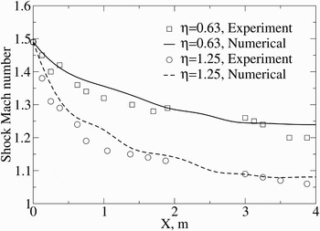
The 1D two-phase code is validated using the experimental results of Sommerfeld (Reference Sommerfeld1985). Here, a 7.81 m long shock tube is considered and is divided into a sequence of three regions: a 2 m long high pressure driver section, followed by a 1.05 m long region filled with ambient air, and last, a 4.76 m long section filled with a mixture of ambient air and dust particles. The Mach number of the incident shock is 1.49, and two different particle mass loading ratio are considered, ν = 0.63 and 1.25. The particles are assumed to be 27 μm in diameter (d p), with a material density, σp = 2500 Kg/m3 and a specific heat, C m of 766 J/Kg-K. Based on trial and error, a resolution of ΔX = 0.01 m is found to suffice for the analysis. After the high pressure section is released, a shock wave propagates into the low pressure region, and attenuates as it propagates through the gas-particle mixture because of momentum and energy loss to the particles. The shock wave Mach number as it attenuates with distance is of interest, and the numerical predictions are presented in Figure 20 along with the experimental data from Sommerfeld (Reference Sommerfeld1985). As evident, the numerical predictions are in good accordance with the experiments. In the far downstream regions (X > 3.5 m) the shock wave tends to attain an equilibrium Mach number as it propagates through the gas-particle mixture, in accordance with results of Sommerfeld (Reference Sommerfeld1985). Furthermore, as expected, for a higher particle mass loading ratio (ν), the equilibrium shock Mach number is lower due to the greater momentum and energy loss from the shock wave to the particles. These results validate the 1D two-phase code for applications of the like.
Shock Mach number as it propagates through a dust-gas suspension. Experimental results are from Sommerfeld (Reference Sommerfeld1985).