Implications
This review contributes to the ongoing efforts for enhancing animal health and sustaining livestock production. By providing an overview of the state-of-the-art in modelling host–pathogen interactions, this review aims to give relevant insight into the contributions and shortcomings of current mathematical models in enhancing our understanding of animal responses to pathogen challenge and for devising appropriate surveillance and control strategies to improve these responses. Combining existing and upcoming modelling approaches with current advances in the acquisition of biological data may serve as a road map for creating a new generation of models that play a fundamental role in combating disease in livestock.
Introduction
The increasing demand for more and healthier food and rising concerns about emerging livestock diseases brought on by climate and pathogen resistance to pharmaceuticals and infrastructure change have placed animal health high on the priority list of livestock production (Perry and Grace, Reference Perry and Grace2009; Department of the Environment, Food and Rural Affairs (Defra), 2010; Simm, Reference Simm2010). Research underpinning our understanding of how animals respond to pathogen challenge and how to improve this response has never been of greater importance. An animal's response to infectious pathogens is a complex interaction of properties of the host, pathogen and environment, and therefore requires contributions from research across a range of disciplines including different branches of biology, epidemiology and environmental science. Over the recent years, more and more mathematical modellers have been employed to study host–pathogen interactions, although the focus has been primarily on modelling immunological processes relevant to human diseases. In contrast, the application of mathematical models to address issues concerning animal health has been relatively sparse.
The aim of this review, written from the perspective of a mathematician working with animal scientists over several years, is to illustrate how mathematical host–pathogen interaction models can contribute to enhancing our understanding of animal responses to pathogens and ultimately help in improving animal health. This will be achieved by outlining the general role of mathematical models in a field dominated by experimental data and by providing some insight into various types of host–pathogen interaction models that differ in their objectives and approaches. Concrete examples will serve to illustrate how different assumptions, concepts and methodologies are implemented into quantitative models and how they can be applied to address important animal health issues. This review is targeted not only towards animal scientists who seek to better understand how mathematical models work and what they can achieve, but also towards modellers who are interested in finding out about modelling approaches that are outside their area of expertise. Ultimately, this review aims to shed light on a potential new approach to tackle animal diseases that uses modelling to integrate theory and experiments.
The need for mathematical host–pathogen interaction models
Complementing empirical studies
The wealth of data from large-scale field studies and small animal models (e.g. mouse or rat) collected in the past decades has substantially improved our understanding of a variety of factors influencing host response to pathogens. Recent advances in molecular and genomic tools have added another dimension to our knowledge base, by providing a detailed insight of the genes and pathways involved in the host immune response. However, results from empirical studies are often limited in scope and validity as they are constrained by physical boundaries. The stark contrast between the large body of research findings and the sparse translation of these findings into practical disease control strategies points to substantial knowledge gaps that need to be overcome. Successful disease control strategies not only require knowledge about individual components of the host or pathogen dynamics, but also some understanding of the system as it functions as a whole (Perelson, Reference Perelson2002).
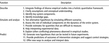
Throughout history, the language of mathematics has proven well suited for integrating diverse empirical findings into a holistic quantitative framework (Morel, Reference Morel1998; Nowak and May, Reference Nowak and May2000; Perelson, Reference Perelson2002). Mathematical models have the benefit over empirical studies that they are free from physical constraints, thus enabling to test a wide spectrum of scenarios that may be difficult to test experimentally. The possibility to calculate the state of all system components represented in the model for any desired duration of time and at any desired frequency may provide the information needed to explain the phenomena observed in empirical studies in which only limited amounts of measurements can be taken. The models thus not only help to test hypotheses emerging from experimental studies, but can also reveal and fill important knowledge gaps leading to the generation of new hypotheses that can be tested in future experiments. Table 1 lists diverse generic functions of mathematical models that have proven useful in existing host–pathogen interaction models, some of which will be described with concrete examples provided here.
Functions of mathematical/computational models of host–pathogen interactions

Help in devising surveillance and control strategies
The importance of mathematical and computational models of immune system dynamics for the development and testing of pharmaceuticals is evident, and the majority of published models of human diseases have been developed for this very purpose. Less attention has been given to reflect how host–pathogen interaction models could prove useful for devising control strategies for diseases in animals. Decisions about which animals should be diagnosed, vaccinated, treated or selected for breeding are generally based on observable biomarkers (e.g. acute phase proteins or other plasma proteins, faecal egg counts (FECs) for parasite infections, somatic cell counts for mastitis, etc.). Although some biomarkers relate to a particular immune response process (e.g. specific antibodies related to the humoral response), others (e.g. FEC and weight gain) are the cumulative result of a variety of interacting processes related to pathogen, host and environment. No biomarker alone can predict or identify animals that are most susceptible or most severely infected with 100% accuracy. Mathematical host–pathogen interaction can describe the underlying biological processes related to specific biomarkers and elucidate how these processes change over time and relate to other key processes (and thus to other potential biomarkers). The modelled relationships could further lead to the proposition of new potential biomarkers related to other important processes. In addition, as models provide time trends of infection characteristics, they could be used to predict the optimal timing and frequency at which biomarkers should be applied to enhance the accuracy of disease diagnostics and predictions of genetic risk of infection and selection response or treatment efficacy.
Three categories of host–pathogen interaction models
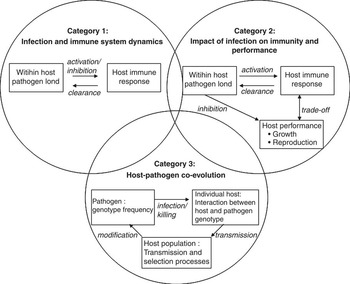
As illustrated in Figure 1, most host–pathogen interaction models can be assigned to one of three categories depending on the questions addressed and the experimental evidence incorporated. The first category comprises the large group of mathematical models that describe the within-host infection and immune system dynamics. The model presented in Example 1 falls into this category. The aim of these models is to synthesise information obtained from diverse pathological and immunological studies into a holistic quantitative framework and use this to gain insights into how specific components of the pathogen and/or immune system function and interact. These types of models find their application mainly in the development and testing of pharmaceuticals.
Schematic diagram of the three alternative categories of existing host–pathogen interaction models. The categories differ in the questions addressed by the models, the biological principles incorporated, the choice and representation of model components and in the methodology. The categories generally correspond to different research disciplines, although methodologies may overlap.

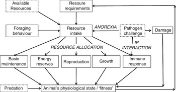
Schematic diagram of processes included in host–pathogen interaction models belonging to category 2. Not all processes/attributes are included in each model. Solid boxes refer to attributes of the animal and dashed boxes refer to attributes of the animal's environment. ANOREXIA, RESOURCE ALLOCATION and IP INTERACTION refer to biological processes represented in (some of) the models. For further explanation, see text.

The second category of models addresses the relationship between immune functions and other biological processes related to survival or production. One common assumption underlying these models is that all biological processes demand nutritional resources and that trade-offs occur between mounting an (or alternative types of) immune response(s) and maintaining fitness or production levels when resources become scarce (Sheldon and Verhulst, Reference Sheldon and Verhulst1996; Lochmiller and Deerenberg, Reference Lochmiller and Deerenberg2000). These types of models arise in evolutionary ecology or livestock production science, in which the focus is not only on the impact of infection on animal health but also on the undesirable side effects related to reproduction and production (e.g. growth rate and milk yield). The model presented in Example 2 falls into category 2.
The third category of host–pathogen interaction models deals with the question of how the interactions between hosts and pathogens affect their co-evolution. These models are important for anticipating the long-term impact of control strategies that alter host and pathogen genetics, such as, for example, the use of anthelmintics to control parasitism, which has resulted in the emergence of anthelmintic-resistant parasites and increased host susceptibility (Sangster, Reference Sangster1999; Jackson and Coop, Reference Jackson and Coop2000). The methodology for models belonging to category 3 differs from those of the other categories, as they concentrate less on the dynamic processes during infection of an individual host, but more on the transmission of pathogens and resulting evolutionary processes in the population. These models are more closely related to epidemiological models and merit a review on their own (e.g. Woolhouse et al., Reference Woolhouse, Webster, Domingo, Charlesworth and Levin2002). In this review, I will focus on models that describe the host–pathogen interaction within individual hosts, that is, models belonging to the first two categories.
Category 1: models of infection and immune system dynamics
Overview of published models for animal diseases
In contrast to the vast amount of epidemiological models that describe the spread of infection between animals and predict disease prevalence and severity in the population, models that study the dynamics of infections in individual animals are relatively scarce. Although most epidemiological models incorporate expressions for the disease progression within animals (e.g. from latent infected to diseased to recovered state in compartmental models for micro-parasitic infections or more explicit descriptions of the life cycle of macro-parasites within and outside the host (Anderson and May, Reference Anderson and May1991)), they will not be considered here as they aim to address questions concerning disease prevalence in the population rather than in individual animals. Published models that concentrate on the within-host dynamics of infections exist for nematode infections in ruminants (Louie et al., Reference Louie, Vlassoff and Macckay2005; Vagenas et al., Reference Vagenas, Bishop and Kyriazakis2007a and Reference Vagenas, Bishop and Kyriazakis2007b), gut and mammary gland infections in cattle caused by Escherichia coli and other bacterial infections related to mastitis in cattle (Oltenacu and Natzke, Reference Oltenacu and Natzke1976; Detilleux, Reference Detilleux2004; Detilleux et al., Reference Detilleux, Vangroenweghe and Burvenich2006; Wood et al., Reference Wood, McKendrick and Gettingby2006a and Reference Wood, McKendrick and Gettingby2006b; White et al., Reference White, Schukken, Dogan, Green, Döpfer, Chappell and Medley2010) and porcine reproductive and respiratory syndrome (PRRS) in pigs (Doeschl-Wilson and Galina-Pantoja, Reference Doeschl-Wilson and Galina-Pantoja2010).
PRRSV (virus) infection (see Example 1)
Given the great economic importance of PRRS in many pig producing countries worldwide, PRRSV infection dynamics have been studied extensively in field and laboratory experiments (Zimmerman et al., Reference Zimmerman, Benfield, Murtaugh, Osorio, Stevenson and Torremorell2006). However, many fundamental questions remain unanswered that prevent the development of effective disease control strategies. The wealth of experimental evidence offers a great opportunity for mathematical models to combine the accumulating knowledge into a holistic quantitative framework.
A first step towards this goal, that is, a simple model for PRRSV infection dynamics, is outlined in detail in Example 1. The model describes how pathogen load, severity of infection and target cell numbers change over time in the absence of an immune response. For a more comprehensive model of PRRSV infection that includes immune response mechanisms, see Doeschl-Wilson and Galina-Pantoja (Reference Doeschl-Wilson and Galina-Pantoja2010). The example presented here not only aims to show how findings from various empirical studies can be combined into a quantitative model (Table 1, point 1) but also illustrates that even very simple mathematical models can produce valuable scientific insights. In particular, discrepancies between model predictions and empirical observations point towards missing system components of great importance that warrant further experimental investigations and model development (Table 1, points 4 and 10).
Example 1: modelling host–virus interaction for the PRRSV infections in pigs
Questions arising from empirical studies
PRRS is an endemic viral pig disease causing reproductive failure in pregnant sows and respiratory disease with an often fatal outcome in growing pigs. A hallmark of PRRSV infection and reason for lack of efficient control to date is the unusual pathogenesis and the atypical immune response it invokes (Murtaugh et al., Reference Murtaugh, Xiao and Zuckermann2002). PRRSV targets primarily a subpopulation of macrophages in the lung and other tissues that have reached a specific stage of differentiation that renders them permissive to the virus (Duan et al., Reference Duan, Nauwynck and Pensaert1997; Gaudrealt et al., Reference Gaudrealt, Rowland and Wyatt2009).
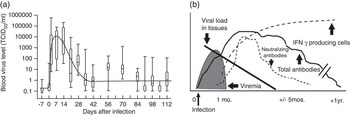
PRRSV infection is characterised by an atypical pathogenesis consisting of a prolonged acute phase lasting for 1 month or longer, with peak virus levels in the blood and lung between 7 to 14 days post infection and followed by a persistent infection in the lung and lymphoid tissues that clears for most animals within 150 days post infection (Allende et al., Reference Allende, Laegreid, Kutish, Galeota, Wills and Osorio2000), but can last in some (especially younger) pigs for several months or years (Lopez and Osorio, Reference Lopez and Osorio2004; Figure 3a).
Time trends for virus load and immune responses observed in empirical studies. (a) Blood virus levels in pigs (n = 16) infected with a virulent strain of PRRSV in the experiment of Mulupuri et al. (Reference Mulupuri, Zimmerman, Hermann, Johnson, Cano, Yu, Dee and Murtaugh2008). The horizontal bars in the box-whisker plots represent the mean, boxes represent the 75th percentile and whiskers extend to minimum and maximum values. (b) Scheme of temporal sequence of events after infection with PRRSV, adapted from Lopez and Osorio (Reference Lopez and Osorio2004); PRRSV = porcine reproductive and respiratory syndrome virus.

Compared with other common viruses, PRRSV fails to elicit any of the typical innate immune response mechanisms (van Reeth and Nauwynck, Reference Van Reeth and Nauwynck2000; Murtaugh et al., Reference Murtaugh, Xiao and Zuckermann2002), and the adaptive immune response is delayed and weak (Molitor et al., Reference Molitor, Bautista and Choi1997; Mulupuri et al., Reference Mulupuri, Zimmerman, Hermann, Johnson, Cano, Yu, Dee and Murtaugh2008; Figure 3b).
The results of empirical studies thus raise the following question that (together with other questions) has been addressed by the mathematical model of Doeschl-Wilson and Galina-Pantoja (Reference Doeschl-Wilson and Galina-Pantoja2010) and is described below.
What causes the decline in virus load during the acute phase of the infection before the onset of the adaptive immune response?
The mathematical model
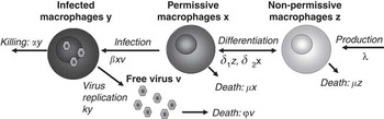
The model describes the interaction between a replicating virus and host alveolar macrophages, the primary site of PRRSV infection, during the acute phase of infection, before the onset of the adaptive immune response (i.e. no VN antibodies and cytotoxic T-cells). The basic model for host–virus interaction contains four variables: uninfected, non-permissive macrophages z, uninfected permissive macrophages x, infected macrophages y and free virus particles v. It is assumed that uninfected non-permissible macrophages z are produced at a constant rate λ, become activated towards a PRRSV permissive state at a rate δ 1z and die at a rate μz. Permissive uninfected macrophages x return to a non-permissive state at a rate δ 2x, die at a rate μx and become infected by PRRSV at a rate βxv. Infected cells die at a rate αy, with α ⩾ μ. Free virus is produced by infected cells at rate a κy and decays at a rate φv. These assumptions are graphically captured in Figure 4 and lead to the following system of ODEs (1).

Schematic representation of the host–pathogen interaction model of porcine reproductive and respiratory syndrome in Example 1. For further explanation, see text.

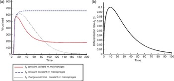
Mathematical stability analysis at the system's steady states shows that there are two possible outcomes for system (1 for system (1) (described by two equilibrium points): either the infection will not be able to establish itself in the host or it will converge to a persistent state with positive viral load (although viral load may be too low to be maintained in reality), as shown in Figure 5a and b. The characteristic of most interest to the first question above is that a decline in virus load to low levels as shown in Figure 5a and observed in empirical studies is only possible if the total number of macrophages decreases substantially. This, however, contradicts empirical findings, which suggest that macrophage numbers in infected tissues remain constant during the time course of infection (Labarque et al., Reference Labarque, Van Gucht, Nauwynck, Van Reeth and Pensaert2003; Xiao et al., Reference Xiao, Batista, Dee, Halbur and Murtaugh2004). Applying the additional constraint that macrophages are replenished at a rate corresponding to a constant number of macrophages leads to a new persistent equilibrium. However, it is straightforward to prove that this equilibrium corresponds to a high virus load (Figure 5a). Hence, the model predicts that a decline in virus load, as observed in empirical studies, would not be possible under the assumptions incorporated in our model, that is, in the absence of immune response and a constant influx of new macrophages to maintain macrophage numbers constant. The results thus suggest that there are other important system components that need to be included in the model.
Predicted virus load profile for the PRRS model (1) with different assumptions concerning macrophage differentiation rate and total number of macrophages (a) and plot of the differentiation rate of lung macrophages, when assumed that it changes over time (b). Implementing this function into model (1) produces the dotted line for virus load shown in panel a.

One possible mechanism that may affect the trend in virus load during the acute phase of infection is that macrophages may become less permissive during the time course of infection. Macrophage permissiveness over time has indeed been assessed in an in vitro infection experiment (Gaudrealt et al., Reference Gaudrealt, Rowland and Wyatt2009), but was found to increase within the first 5 days post infection. However, this time frame corresponds to the early stage of acute infection in which virus load still increases. Up to now, no published experimental study has investigated macrophage permissiveness over a sufficiently long time period to detect whether permissiveness decreases over a longer time period. The advantage of mathematical models is that they allow assessment of the outcome of hypothetical scenarios. Replacing the constant differentiation rate δ 1 in model (1) by the function δ 1(t) = at bexp(−ct), with parameters a, b and c describing fast differentiation rates at the early stages and slow differentiation rates at the later stages of infection (Figure 5b), indeed produces a reduction in virus load similar to those observed in experiments (Figure 3a).
This hypothesis is currently assessed in a laboratory study and stimulated a fruitful collaboration between mathematicians and molecular scientists. Preliminary results from the in vitro experiment confirm the hypothesis that macrophage permissiveness initially increases and declines after about 6 days post infection, and they also provide further insights into the underlying mechanisms responsible for this decline from which more accurate estimates for the differentiation rate δ 1(t) in the above model can be derived (Reyes-Umana, Reference Reyes-Umana2010).
Gastrointestinal parasitism in ruminants
An approach different from the PRRS infection model has been adopted for host–pathogen interaction models of gastrointestinal parasitism in ruminants, which, like all (epidemiological) macro-parasitic infection models, describe the life cycle of the parasite within the host from the intake of larvae to their establishment in the gastrointestinal tract and finally the production and excretion of larval eggs (Bishop and Stear, Reference Bishop and Stear1997; Louie et al., Reference Louie, Vlassoff and Macckay2005; Vagenas et al., Reference Vagenas, Bishop and Kyriazakis2007a and Reference Vagenas, Bishop and Kyriazakis2007b). The model of Vagenas et al. (Reference Vagenas, Bishop and Kyriazakis2007a and Reference Vagenas, Bishop and Kyriazakis2007b), presented in detail in Example 2, describes the impact of parasitism on both host immunity and performance, and therefore belongs to category 2. However, as infection and immune system dynamics have been modelled in a similar way as in all of the above models, the model is also partly considered here. In particular, host–pathogen interactions are described by the impact of larval challenge on the acquisition of immunity of the host (which are simple functions of the cumulative larval intake in the above-mentioned models), as well as by the influence of the host genotype and physiological or immune status on larval establishment, worm mortality and fecundity. Rather than containing explicit descriptions of individual immune processes, the models describe the effects of the host immune response on different stages of the parasite life cycles.
Model application consists of assessing the influence of diverse factors on the outcome of infection and of identifying key biological uncertainties for which field data are required. For example, Louie et al. (Reference Louie, Vlassoff and Macckay2005) established that parameters determining larvae establishment have the greatest influence on peak parasite burden, whereas parameters affecting mortality and fecundity had greater influence on the duration of the infection. Vagenas et al. (Reference Vagenas, Bishop and Kyriazakis2007a) also identified larval establishment rate (E) as a key parameter determining the time trend of infection. In addition, they quantified the impact of different challenge doses, nutritional regimes (ranging from protein-rich to protein-scarce diets) and of the host genotype on parasite burden and other traits of interest.
Despite differences in the actual model equations, existing models of gastrointestinal parasite infections in ruminants are similar in that they are hypothesis driven. In other words, they aim to provide an understanding of the influence of various factors on the infection dynamics, rather than to provide quantitatively accurate representations of individual immune processes. Obtaining accurate estimates of the model parameters and fitting the models to existing data may prove challenging as many key model parameters are defined on conceptual grounds (e.g. genotypes for growth or resistance) rather than representing measurable entities.
Example 2: modelling growth and immune response to gastrointestinal parasite challenge in immunologically naive lambs
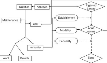
In order to assess the influence of host genetics and nutrition on gastrointestinal parasitism in lambs, Vagenas et al. (Reference Vagenas, Bishop and Kyriazakis2007a) developed a deterministic, dynamic simulation model that describes the growth and immune response of initially naive lambs facing pre-defined levels of nematode challenge. A schematic diagram of the basic concepts and rules for the host–pathogen interaction is shown in Figure 6. Inputs to the model are (genetically controlled) growth and resistance attributes of the host, feed quality, various parasitological parameters and daily larval intake. The model is built upon a nutritional framework, that is, all biological processes represented by the model are described in terms of nutrient requirements and nutrients allocated to the individual processes. For example, the host's growth genoytpe determines the desired nutrient intake, whereas the intake of parasitic larvae and established adult worms are assumed to result in nutrient loss for the host. The host counteracts this loss by mounting an immune response, which affects, in addition to the nutrient loss caused by larvae, the establishment rate of incoming larvae, mortality rate of adult worms and fecundity of female worms. Nutrient scarcity and the dilemma in nutrient allocation arises as a consequence of anorexia, which is modelled as a function of worm mass. Outputs include feed intake, growth rate and body composition, as well as worm burden and FEC.
Schematic diagram of the host–parasite interaction model. Rectangular boxes indicate the fate of the ingested protein, rounded boxes indicated host–parasite interactions and diamond boxes indicate key quantifiable parasite life cycle stages. Dotted lines refer to the parasite life cycle. The figure was published in Vagenas et al. (Reference Vagenas, Bishop and Kyriazakis2007a).

The model consists of a large number of mathematical equations describing changes in the model variables according to heuristically derived relationships. The time trends in the model variables are then described by first-order difference equations (i.e. X(t + 1) = X(t) + dX*Δt), where a time step Δt of 1 day was used. Critical equations are those describing the rates of host-controlled establishment, fecundity and mortality of adult worms. These are sigmoidal functions of cumulative larval intake and relate the biological processes to nutrient requirements. For example, larval establishment (E) is described by

where ε min and ε max are minimum and maximum rates of establishment, respectively, and PRQImm and PACImm are protein required and allocated to immunity, respectively, KE is a scaling parameter and  is the scaled larval intake.
The model, and its extension to a population level, satisfied many of the functions listed in Table 1 (Vagenas et al., Reference Vagenas, Bishop and Kyriazakis2007a, Reference Vagenas, Bishop and Kyriazakis2007b and Reference Vagenas, Doeschl-Wilson, Bishop and Kyriazakis2008; Doeschl-Wilson et al., Reference Doeschl-Wilson, Vagenas, Kyriazakis and Bishop2008). By describing all biological processes in a nutritional context, the interactive effects of host genetics and nutrition on gastrointestinal parasitism, which are difficult to study experimentally, could be explored in silico (Table 1, points 1, 5, 6 and 7). The host–pathogen interaction model for individual animals was used to assess the time trends and severity of gastrointestinal parasitism in sheep of different growth and resistance characteristics, and kept in environments that vary in the provision of nutrients and exposure to parasites (Vagenas et al., Reference Vagenas, Bishop and Kyriazakis2007b). One of the benefits of this model is that it provides time trends for observable output traits (e.g. growth rate and FEC), thus allowing assessment of the impact of different control factors at different stages of the infection (Table 1, points 11 and 12).
E. coli infections in the gut and mammary gland of cattle
Reflecting on the huge impact of E. coli on cattle health and milk production, and in some cases also on human health (for E. coli O157), several mathematical models exist for the within-animal infection dynamics of E. coli. Wood et al. (Reference Wood, McKendrick and Gettingby2006a) developed a stochastic simulation model that describes the ingestion process and the resulting bacterial population dynamics through simple birth–death and migration processes between different compartments in the bovine gut. Intensive literature search for parameter estimates and model fitting to experimental data showed that a variety of experimental features could be reproduced by the model (e.g. shedding duration and bacterial distributions in different gut compartments), but it also revealed important knowledge gaps that prevent the accurate prediction of bacterial time trends. Despite some uncertainties in the parameterisation, the model results suggest that although ingestion events in individual animals are expected to be rare, a small number of ingestion events would be sufficient to maintain the infection within an animal. This insight was used in a subsequent paper in which the model was used to explore the efficacy of diverse control strategies (Wood et al., Reference Wood, McKendrick and Gettingby2006b).
A more data-driven approach was adopted by Detilleux et al. (Reference Detilleux, Vangroenweghe and Burvenich2006), who modelled the acute inflammatory response to E. coli of the bovine mammary gland. Their deterministic model consists of three relatively simple ordinary differential equations (ODEs) that describe the interactions between bacteria, milk somatic cells and blood leucocyte densities. By fitting the model equations to data from challenge studies, accurate estimates for the model parameters were obtained, and the influence of different experimental conditions (e.g. vaccinated and non-vaccinated animals, different bacterial strains) on the model parameters was assessed. The model also provided a threshold measure for the minimum milk cellular density necessary to protect the gland against E. coli. A similar approach (albeit a different model) had been applied in an earlier model of the same lead author to obtain an estimate of the minimum concentration of blood neutrophils necessary to decrease the concentration of other bacteria in mastitic milk (Detilleux, Reference Detilleux2004). These studies show that even relatively simple models can produce accurate quantitative predictions and provide valuable insight into the role of different key parameters. However, simple models may not be able to capture all relevant phenomena observed in real studies. In this case, infection dynamics were adequately described for the acute stage of the infection but the model did not capture the persistent stage.
A model that is able to describe infection processes at any stage of mammary E. coli infection was recently developed by White et al. (Reference White, Schukken, Dogan, Green, Döpfer, Chappell and Medley2010), with the objective to determine the processes that lead to either transient or persistent infections. Their model includes a more detailed description of bacteria (distinguishing between intracellular E. coli and E. coli in milk), immune response mechanisms (including pro-inflammatory and inhibitory cytokines and concentrations of macrophages and polymorphonuclear cells) and environmental factors (impact of lactation on cell numbers) than other models. More complex models generally require more parameters. Parameter estimates were derived by using a combination of literature studies and fitting the model to data from individual cows with transient and persistent infections. On the basis of the results of the fitted models, the authors established the most likely causes of divergent outcomes (i.e. clearance or persistence).
In summary, there are relatively few models describing the within-host infection dynamics for specific diseases in animals. Existing models vary in their approach and in the level of detail in which biological processes are represented, but most models implement a very crude description of the host immune response and its effect on within-host–pathogen load.
Overview of published models for basic immune processes relevant for diseases in humans
In contrast to the few mathematical models that describe the dynamics of infections in animals, the application of mathematical modelling in the study of immune system dynamics in general and applied to human diseases is well established. The abundance of published immune response models can be partly attributed to the recent explosion of available experimental data, combined with the recognition that an in-depth understanding of the immune system with all its dynamic interactions cannot be deduced from experiments alone (Yates et al., Reference Yates, Chan, Callard, George and Stark2001). In immunology, mathematical models have adopted the role of providing the (quantitative) theoretical framework for interpreting the wealth of available immunological data. In addition, the value of mathematical models in advancing the understanding of the immune system and in the development and in silico testing of treatment strategies has been convincingly described by models of human immunodeficiency virus (HIV) and some other infections in humans that emerged in the 1990s (see reviews by Morel, Reference Morel1998; Perelson, Reference Perelson2002; Davenport et al., Reference Davenport, Ribeiro, Zhang, Wilson and Perelson2007). The success story of the early models has sparked much collaboration between mathematicians and immunologists since.
The extreme complexity of the immune system and the vast variety of available data representing different system components are mirrored by the great diversity of available mathematical models. Detailed information about various types of models of immune system dynamics published in the immunological and mathematical literature is beyond the scope of this review, but can be found in several excellent reviews (e.g. Morel, Reference Morel1998; Nowak and May, Reference Nowak and May2000; Yates et al., Reference Yates, Chan, Callard, George and Stark2001; Perelson, Reference Perelson2002; Louzoun, Reference Louzoun2007; Kirschner and Linderman, Reference Kirschner and Linderman2009).
Existing models of immune system dynamics vary between those addressing basic immunological phenomena, such as antigen recognition or development of immune cells and effector mechanisms (e.g. Perelson and Wiegel, Reference Perelson and Wiegel1981; Antia et al., Reference Antia, Ganusov and Ahmed2005; Souza-e-Silva et al., Reference Souza-e-Silva, Savino, Feijóo and Vasconcelos2009), models that are generic for virus or bacterial infections (e.g. Antia and Koella, Reference Antia and Koella1994; Antia et al., Reference Antia, Koella and Perrot1996; Nowak and Bangham, Reference Nowak and Bangham1996; Kleinstein and Seiden, Reference Kleinstein and Seiden2000; Pugliese and Gandolfi, Reference Pugliese and Gandolfi2008) and models that focus on a particular (mostly human) disease of interest (e.g. Marchuck et al., Reference Marchuck, Petrov, Romanyukha and Bocharov1991; Wodarz, Reference Wodarz2003; Kosmrlj et al., Reference Kosmrlj, Read, Qi, Allen, Altfeld, Deeks, Pereyra, Carrington, Walker and Chakraborty2010; Smith and Ribeiro, Reference Smith and Ribeiro2010). Models differ widely in the level of detail and the temporal and spatial scales at which immune processes are represented as well as in their methodologies. Many (in particular, early) immunological models are more conceptual, focusing on a phenomenological description of the time course of infection that results from the interaction of a relatively small number of components (e.g. antigen with antibodies, T-cells or memory B cells; Perelson and Wiegel, Reference Perelson and Wiegel1981; Wodarz et al., Reference Wodarz, Lloyd, Jansen and Nowak1999; Wodarz, Reference Wodarz2003; Pugliese and Gandolfi, Reference Pugliese and Gandolfi2008). In these models, the description of the individual system components and their interactions can be simple (e.g. constant proliferation rates, ignoring time delay or spatial distribution) and model variables and parameters are often unscaled or described in arbitrary units (as in Example 1). Nevertheless, the dynamic properties of the simplistic model systems often mimic the complex dynamics observed in the real world, demonstrating the fact that complex behaviour can emerge from simple interactions between few components.
Increasing acquisition of data that produce detailed insight into the fine building blocks of the immune system, together with the shift from a reductionist to a systems view of biology (Kitano, Reference Kitano2002), also raises the demand for a shift in mathematical modelling. Traditional conceptual approaches are replaced by more data-driven approaches and mathematical systems with few components giving way to large networks. Citing Louzoun (Reference Louzoun2007), ‘mathematical modelling in immunology is becoming more and more molecular’.
One hallmark of mathematical modelling of immune system dynamics is the incredibly rich repertoire of mathematical methodology applied, which has evolved over time in synchrony with the acquisition of new data. The advances in the collection, storage and analysis of biological data are also applicable to livestock diseases. Some of the most common approaches, which are relevant to the development of host–pathogen interaction models for livestock diseases, are outlined in the section ‘Overview of mathematical methodologies used in host–pathogen interaction models’.
Category 2: models that consider the impact of infection on health and productive functions
An accurate understanding of the immune system dynamics is vital for the development of pharmaceuticals, but for the sustainability of livestock production a deep understanding of the relationship between health, reproduction and production traits is equally important. These questions are the focus of models belonging to category 2, which arise mainly from evolutionary ecology and livestock production science. Evolutionary ecologists are interested in understanding the factors influencing an animal's ‘decision making’, in particular when investment in immunity competes with investment in reproduction or other survival traits (Medley, Reference Medley2002; Houston et al., Reference Houston, McNamara, Barta and Klasing2007). Ultimately, the understanding will provide insight into the evolution of immune and survival functions in animal species. In contrast, livestock production scientists are more interested in predicting the influence of infection on productive traits (Lescourret and Coulon, Reference Lescourret and Coulon1994), in anticipating the consequence of genetic selection on animal health and production and in determining the role of environmental factors (e.g. pathogen challenge and nutrition) on the health–production relationship. Their ultimate aim is to obtain the necessary understanding for minimising the detrimental effects and side effects of disease on animal health and other traits of interest.
Basic principles of models in category 2
A common assumption underlying the majority of host–pathogen interaction models of category 2 is that immunity, like all biological processes, requires resources (e.g. protein and energy). Resource scarcity, either resulting from environmental conditions (e.g. food shortage due to seasonal effects) or from infection-induced anorexia (Exton, Reference Exton1997; Ayres and Schneider, Reference Ayres and Schneider2010) causes a trade-off between diverse resource-demanding functions. The observed response of an animal in terms of immunity, reproduction and/or production is then the outcome of an individual's distribution of resources between different competing processes.
The schematic diagram of Figure 2 illustrates how the above-described nutritional framework is incorporated in the host–pathogen interaction models belonging to category 2. Despite the common conceptual approach, models differ in the actual components included in the models (e.g. no model considers all of the listed body functions in the nutrient allocation simultaneously and only a few models included infection-induced anorexia), in the representation of pathogen challenge (e.g. pathogen dose, incoming larvae and infection pressure) and resources (e.g. energy or protein), in the resource allocation rule and in the description of the interaction between pathogens and the host's immune response.
Host–pathogen interaction models of category 2 in evolutionary ecology
Host–pathogen interaction models in evolutionary ecology aim to determine the optimum host defence strategy (mainly allocation of resources) corresponding to minimum resource requirements (Shudo and Iwasa, Reference Shudo and Iwasa2001), maximum chance of survival (e.g. McNamara and Buchanan, Reference McNamara and Buchanan2005; Houston et al., Reference Houston, McNamara, Barta and Klasing2007) or maximum number of offspring (e.g. Medley, Reference Medley2002). They assess how optimum allocation depends on various factors such as nutrient availability, pathogen challenge or the physiological status of the host, with the aim to explain contrasting phenomena observed in field studies.
Examples of evolutionary ecology models applying the principle of trade-offs to host–pathogen interactions for an individual animal include the model of Medley (Reference Medley2002), who showed that the optimal defence strategy of a host exposed to a constant parasite challenge may be to tolerate rather than to clear parasites. The model also investigates how the optimum level of parasites to be tolerated depends on host resource acquisition, on parasite pathogenicity and on host exposure level to the parasite. The model provides theoretical support for the hypothesis emerging from field observations that non-zero parasite burden could be beneficial to the host (Behnke et al., Reference Behnke, Barnard and Wakelin1992), and also offers some explanation for the observed variations in parasite burdens between hosts and parasite species.
Houston et al. (Reference Houston, McNamara, Barta and Klasing2007) applied the principle of nutrient allocation to examine the trade-off between accumulating energy reserves to avoid starvation and investing in immunity to avoid death by disease for animals exposed to changing environmental conditions. Their model suggests that the optimal host strategy at a given time depends largely on the host's energy reserves and on the frequency of changes in food availability.
Trade-offs occur not only between immunity and other fitness functions or production, but also between different immune processes, such as between immediate or delayed responses (Segel and Bar-Or, Reference Segel and Bar-Or1999) or between cellular and humoral immune responses (Bankroft et al., Reference Bankroft, Else and Grencis1994). For example, mouse experiments showed that different doses of the same pathogen or pathogens with different virulence could lead to divergent differentiation of Th0 cells into either Th1 or Th2 cells activating cellular or humoral immune response mechanisms, respectively (Janeway et al., Reference Janeway, Travers and Walport1999). This motivated Shudo and Iwasa (Reference Shudo and Iwasa2001) to develop a mathematical model to investigate whether different dominance patterns between immune response mechanisms could be inferred from energy costs associated with different defence strategies. Weighting the energy cost of defence associated with different types of immune responses against inflicted damage, their model showed that response mechanisms that require no or little time delay would be beneficial over delayed response if pathogen dose and virulence are high, thus supporting the experimental findings.
Although the processes implemented into these models differ, the models share the underlying principle of trade-off arising from resource scarcity and partitioning. In addition, all of these models are represented as systems of ODEs (see section ‘Overview of mathematical methodology’ below).
Host–pathogen interaction models of category 2 in livestock science
Generic models for micro-parasitic infections
Host–pathogen interaction models in livestock production science are aimed more at determining the optimal control than optimal host strategy. The underlying assumption of these models is that the host genotype largely determines the nutrient requirements and/or nutrient allocation between different biological processes and that the partitioning rules are known. The models are then used to assess how changes in the animal's genotype (e.g. through genetic selection) or changes in environmental conditions (e.g. different pathogen challenge, nutrient availability or diet composition) affect nutrient intake and allocation and consequently also the observable phenotypes related to health, reproduction and production (e.g. van der Waaij et al., Reference Van der Waaij, Bijma, Bishop and van Arendonk2000; van der Waaij, Reference Van der Waaij2004; Vagenas et al., Reference Vagenas, Bishop and Kyriazakis2007a, Reference Vagenas, Bishop and Kyriazakis2007b and Reference Vagenas, Doeschl-Wilson, Bishop and Kyriazakis2008; Doeschl-Wilson et al., Reference Doeschl-Wilson, Vagenas, Kyriazakis and Bishop2008 and Reference Doeschl-Wilson, Brindle, Emmans and Kyriazakis2009a). In particular, the models aim to shed light on the ongoing debate about how genetic selection influences the relationship between disease resistance and (re-) production (Knap and Bishop, Reference Knap and Bishop2000; Houdijk and Bünger, Reference Houdijk and Bünger2006; Doeschl-Wilson et al., Reference Doeschl-Wilson, Kyriazakis, Vincent, Rothschild, Thacker and Galina-Pantoja2009b). It has been suggested that selection for increased production over the last decades has made animals on average more susceptible to disease as it may draw resources away from immune defence towards costly productive processes when nutrients are scarce (Sheldon and Verhulst, Reference Sheldon and Verhulst1996; Lochmiller and Deerenberg, Reference Lochmiller and Deerenberg2000). However, empirical evidence based on estimates of genetic correlations between health and production traits also exists for the contrary, as reviewed by Rauw et al. (Reference Rauw, Kanis, Noordhuizen-Stassen and Grommers1998).
As described by van der Waaij et al. (Reference Van der Waaij, Bijma, Bishop and van Arendonk2000) and van der Waaij (Reference Van der Waaij2004), it is possible to assess the consequences of genetic selection on the animal's ability to cope with infectious challenge with models that do not include explicit expressions for host–pathogen interactions. Representing host–pathogen interactions simply by the extent to which genotypes for production and fitness can be realised (with high infectious pressure corresponding to low realised production), van der Waaij et al. (Reference Van der Waaij, Bijma, Bishop and van Arendonk2000) showed that selection for observed production could result in increased disease resistance when animals are exposed to constant infection pressure. A later model (van der Waaij, Reference Van der Waaij2004) then described how changes in resource availability and partitioning caused by genetic selection for observed production could affect both the sign and degree of genetic correlations between production and fitness traits.
More recently, Doeschl-Wilson et al. (Reference Doeschl-Wilson, Brindle, Emmans and Kyriazakis2009a) used a generic model for host–pathogen interactions for micro-parasitic infections to explore genetic and nutritional influences on the production–disease resistance relationship over time. The underlying assumption of this model was that the host's genetic capacities for growth and immune response determine its nutrient requirements and preference of allocating nutrients to either process. In addition, nutrient availability (which is reduced due to infection-induced anorexia) and allocation stipulate the extent to which the genotypes are expressed if the animal is challenged by pathogens. The simulations demonstrate that a host's response to pathogen challenge is the result of a complex interaction between host genotypes and the nutritional environment, and that different outcomes to genetic selection could be expected if selection was performed under nutrient-rich or nutrient-scarce conditions (Doeschl-Wilson et al., Reference Doeschl-Wilson, Brindle, Emmans and Kyriazakis2009a). The model also reveals the importance of appropriate timing of measurements on which selection is to be based, as the same selection criteria applied at different time points could lead to different trends in genetic improvement. All models belonging to category 2 mentioned so far are non-specific to any particular type of pathogen and typically represent pathogen challenge, immune response, host genotype and nutrition through single entities with arbitrary units. The objective of these models is to explain general phenomena rather than to accurately predict the outcome for a particular disease.
A specific model for the influence of parasitism on sheep health and production (see Example 2)
To the best of my knowledge, the only (mechanistic) host–pathogen interaction model that explores how pathogen challenge affects both production and health for a particular disease is the model for gastrointestinal parasitism in growing lambs by Vagenas et al. (Reference Vagenas, Bishop and Kyriazakis2007a). As outlined in more detail in Example 2, the model adopts similar principles for nutrient requirements and distribution as the generic model of Doeschl-Wilson et al. (Reference Doeschl-Wilson, Brindle, Emmans and Kyriazakis2009a) to simulate nutrient utilisation, growth, immune status and parasite burden of an infected sheep on a daily basis. One of the main benefits of a disease-specific model over generic models is that the model can provide quantitative predictions for observable growth and resistance traits (e.g. body weight and FECs), which can be compared with existing data. For example, extreme correlations between resistance and growth, similar to those derived from field studies (McEwan et al., Reference McEwan, Mason, Baker, Clarke, Hickey and Turner1992, Reference McEwan, Dodds, Gree, Bain, Duncan, Wheeler, Knowler, Reid, Green and Douch1995) could only be reproduced by the model of Vagenas et al. (Reference Vagenas, Bishop and Kyriazakis2007a and Reference Vagenas, Bishop and Kyriazakis2007b) if underlying traits were genetically related (Doeschl-Wilson et al., Reference Doeschl-Wilson, Vagenas, Kyriazakis and Bishop2008). The results thus point to pleiotropic or linkage effects between underlying growth and resistance mechanisms related to parasitism. In addition, the model offered some explanations with regard to dietary effects on the growth–resistance relationship explored in various field studies (e.g. Greer, Reference Greer2008; Zaralis et al., Reference Zaralis, Tolkamp, Houdijk, Wylie and Kyriazakis2008). The model results suggest that infection-induced anorexia is more likely to be observed when nutrition is rich in dietary proteins (Vagenas et al., Reference Vagenas, Bishop and Kyriazakis2007b), and that genetic correlations between growth and resistance traits are stronger in protein-scarce than protein-rich environments (Vagenas et al., Reference Vagenas, Doeschl-Wilson, Bishop and Kyriazakis2008).
Nutrient intake and allocation as key drivers in models of category 2
Nutrient intake and partitioning are key drivers determining the observed host response to infectious challenge in all models belonging to category 2 (Figure 2). Whereas nutrient intake is either provided as model input or can be predicted based on existing theoretical frameworks (e.g. Kyriazakis and Emmans, Reference Kyriazakis and Emmans1999; Sandberg et al., Reference Sandberg, Emmans and Kyriazakis2006; Kyriazakis and Doeschl-Wilson, Reference Kyriazakis and Doeschl-Wilson2009), all models rely on assumptions concerning how nutrients are partitioned between different body functions that are difficult to verify with experimental data (Friggens and Newbold, Reference Friggens and Newbold2007). It is therefore not surprising that substantial differences exist between nutrient allocation rules adopted in different models. For example, van der Waaij (Reference Van der Waaij2004) assumed that nutrient partitioning is a genetic characteristic of the host, independent of the host's physiological status or level of infectious challenge. In the models of Vagenas et al. (Reference Vagenas, Bishop and Kyriazakis2007a and Reference Vagenas, Bishop and Kyriazakis2007b) and Doeschl-Wilson et al. (Reference Doeschl-Wilson, Brindle, Emmans and Kyriazakis2009a), nutrient allocation to growth and immunity is status- and genotype-dependent and based on the relative nutrient requirements for either process. In contrast, Medley (Reference Medley2002) proposed that the proportion of resources allocated to the immune response depends on the pathogen load and does not exceed a fixed proportion of the total resources available to the host. Given the importance of nutrient allocation for determining the health–production relationship, more research efforts to come up with a unified framework would be warranted. These could extend existing theoretical frameworks for predicting nutrient partitioning based on empirical observations (Coop and Kyriazakis, Reference Coop and Kyriazakis1999; Houdijk et al., Reference Houdijk, Jessop and Kyriazakis2001; Friggens and Newbold, Reference Friggens and Newbold2007).
Description of host–pathogen interactions in models of category 2
In contrast to the infection models of category 1, all models belonging to category 2 adopt a relatively simplistic description of host–pathogen interactions. In the simplest case, host–pathogen interaction is only indirectly described by the impact of pathogen challenge on the expression of the host genotype (e.g. van der Waaij et al., Reference Van der Waaij, Bijma, Bishop and van Arendonk2000; van der Waaij, Reference Van der Waaij2004) or by the probability of death due to disease (Houston et al., Reference Houston, McNamara, Barta and Klasing2007). Others describe host–pathogen interaction by the impact of pathogen challenge on the immune response alone, ignoring how the immune response affects the within-host pathogen load (e.g. Medley, Reference Medley2002). Conversely, the interactions were also described by the impact of the immune response on the pathogen load (e.g. Shudo and Iwasa, Reference Shudo and Iwasa2001), assuming that the strength of the immune response is constant over the time course of infection and independent of the type or degree of pathogen challenge. Even models that incorporate explicit two-way interactions between the host immune response and within-host pathogen load (e.g. Vagenas et al., Reference Vagenas, Bishop and Kyriazakis2007a; Doeschl-Wilson et al., Reference Doeschl-Wilson, Brindle, Emmans and Kyriazakis2009a) only describe the immune response by a single or few entities representing, for example, the intensity of the immune response or the nutrient requirements for immunity.
Besides the risk of ignoring the role of essential system ingredients, the consequence of this simplistic representation of the immune system is that the models are restricted to exploring qualitative behaviour and trends with regard to the infection dynamics, and have limited predictive power. Currently, a number of models exist that predict the growth and body composition of animals relatively accurately when animals are raised in healthy environments (e.g. Knap, Reference Knap1999; Green and Whittemore, Reference Green and Whittemore2003) or challenged with social stressors (Wellock et al., Reference Wellock, Emmans and Kyriazakis2003). However, to this date, no model exists that can accurately predict how these traits are affected if animals are infectiously challenged (Kyriazakis and Houdijk, Reference Kyriazakis and Houdijk2007).
Including a more detailed description of the immune response into these models would require specification of resource requirements and allocation corresponding to each individual immune process captured by the model. Several studies have shown that estimates for protein and energy requirements for immune processes in animals can be empirically derived (Lochmiller and Deerenberg, Reference Lochmiller and Deerenberg2000; Houdijk et al., Reference Houdijk, Jessop and Kyriazakis2001; Klasing, Reference Klasing2007). The model of Romanyukha et al. (Reference Romanyukha, Rudnev and Sidorov2006) illustrates that empirical estimation of resource requirements for specific immune processes is feasible and can lead to valuable model predictions: after deriving estimates of energy requirements for eight different immune processes relevant in pneumonia infections, their mathematical model could predict whether pneumonia infections will lead to acute or chronic conditions based on energy costs alone. The theoretical frameworks for predicting nutrient partitioning mentioned above may serve as a good basis for deriving quantitative estimates of nutrient allocation to the immunological and other biological processes considered in the models.
Alternative approaches to model the effect of infection on production traits
Not all models belonging to category 2 addressing the relationship between health and production traits are based on biological principles. For example, the two independent simulation models for predicting the impact of mastitis on milk production in dairy cows (Oltenacu and Natzke, Reference Oltenacu and Natzke1976; Lescourret and Coulon, Reference Lescourret and Coulon1994) build upon the results of statistical analyses of mastitis and lactation data from commercial dairy herds rather than upon biological concepts. Although the data-driven models may provide a useful means to investigate the effect of changes in animal characteristics and management on milk production (Lescourret and Coulon, Reference Lescourret and Coulon1994), their scope is limited as extrapolation of model results beyond the conditions captured by the available data is questionable.
Overview of mathematical methodologies used in host–pathogen interaction models
The spectrum of mathematical methodologies applied to model host–pathogen interactions, in particular to model immunological processes, is extremely rich. Different methodologies often generate different kinds of insight, and the choice of the most appropriate methodology for the question at hand may not always be obvious. This section of the review summarises the principles, strengths and weaknesses of the most widely applied mathematical tools in current host–pathogen interaction models.
Systems of differential equations (DEs)
Traditionally, dynamical systems in mathematics are represented by sets of DEs (ODE, if change of system with respect to time is studied and partial DEs, if a spatial component is included). The model in Example 1 is represented through ODEs, and most host–pathogen interaction models in evolutionary biology consist of ODE systems. Equipped with a robust set of mathematical tools to solve and analyse the behaviour of DEs developed by mathematicians over centuries, DEs (in particular, ODEs) have been used widely in models of immune reactions in previous years and are most likely to continue being used in the future for systems comprising a limited number of components. Despite their popularity, DEs have several important limitations: first, non-linearities in the system can cause difficulties in deriving (analytical or numerical) solutions of the DE systems, especially if the system contains a large number of variables, or if parameters are symbolic rather than actual values (which lend themselves to more thorough mathematical analysis). Second, as the variables of DE models describe generally a number or density of specific components (e.g. cells and virus particles), they rely on the assumption that entities are identical. Individual variation, brought on, for example, by genetic heterogeneities of hosts or pathogens or different life histories, is not easily captured by these models. Another limitation of DEs is that they are deterministic and thus only provide information about the average behaviour of a system rather than about the distributions of possible outcomes. In addition, model variables can adopt arbitrary small values that may not be realistic, such as pathogen loads corresponding to <1 pathogen particle, and the modeller is faced with making subjective decisions on how to interpret these values.
Mechanistic stochastic models
Many of these limitations can be overcome by introducing a chance element to the dynamic processes described by the DE models, using stochastic modelling approaches (e.g. Renshaw, Reference Renshaw1991). A chance element can be introduced to the initial conditions (e.g. initial pathogen challenge, host status and time of infection) or to the occurrence of particular events captured by the models. All stochastic models therefore require the use of random number generators and, as every realisation of the model leads to a different prediction, multiple simulations to determine the expected range of behaviour. The models thus provide a distribution of outputs rather than single predictions of the average system behaviour. Stochastic models are particularly useful in scenarios in which chance fluctuations become important, as for example, when pathogen load or immune responses can be eliminated due to stochastic fade-out (Wood et al., Reference Wood, McKendrick and Gettingby2006a; White et al., Reference White, Schukken, Dogan, Green, Döpfer, Chappell and Medley2010). As these models are usually computationally demanding and more difficult to analyse than deterministic models, application of stochastic approaches to model host–pathogen interactions are at present relatively sparse.
Cellular automata (CA) and agent-based models (ABMs)
CA and ABMs are the biological alternatives to the mechanistic DEs and their stochastic equivalents. Rather than applying sophisticated mathematical methods to obtain (analytical or approximate) solutions to a given set of equations representing the entire system dynamics, CA and ABMs simulate (usually simple) local interactions between discrete ‘cells’ (or ‘agents’ in case of ABMs) (Wolfram, Reference Wolfram1994; Bauer et al., Reference Bauer, Beauchemin and Perelson2009). The dynamic evolution of the system is then completely described by the specified rules of interaction. The underlying assumption of these types of models is that complex patterns can emerge from relatively simple sets of interactions between system components, and the aim of these models is therefore to establish the rules that generate similar dynamic behavioural patterns as those observed in real systems. In contrast to the continuous DEs, CA and ABMs are discrete in both time and space.
Originally, CA models were deterministic and consisted of a regular grid of identical cells that assume a finite set of states, which solely depend on the states of the neighbouring cells (Wolfram, Reference Wolfram1994). Although restrictive, the mathematical properties of these types of models were well characterised. Several types of CA models have been developed to model different aspects of the immune system (Celada and Seiden, Reference Celada and Seiden1992; Seiden and Celada, Reference Seiden and Celada1992; Morpurgo et al., Reference Morpurgo, Serentha, Seiden and Celada1995; Zorzenon dos Santos and Coutinho, Reference Zorzenon dos Santos and Coutinho2001; Shi et al., Reference Shi, Tridane and Kuang2008) of which the immune simulator IMMSIM (Kleinstein and Seiden, Reference Kleinstein and Seiden2000) is probably the best known. However, most of these CA models involve essential modifications of the original concepts of CA (e.g. stochastic or continuous CAs and entities can move between sites, etc.).
ABMs are natural extensions of CA models, relying on the same principle that complex dynamic behaviour emerges from local interactions of discrete agents, but applying less restrictive rules. ABMs are stochastic, thus providing a distribution of outputs rather than single predictions of the average system behaviour. As the rules are still simple but less restrictive than the CA rules, ABMs can handle a large number of different immune system agents. Reflecting the trend of increasing data production in experimental immunology, ABMs of immune processes have emerged due to the desire to provide a more comprehensive description of the complex immune network, comprising a large number of interacting entities together with their inherent stochasticity. Examples of existing ABMs of host–pathogen interactions and their pros and cons are discussed in the review of Bauer et al. (Reference Bauer, Beauchemin and Perelson2009). The majority or CA or ABMs model ‘generic’ immune processes rather than specific diseases. ABMs are relatively new in mathematical immunology and to the best of my knowledge have not yet been applied to study the relationship between processes related to health and production.
The main advantage of CAs and ABMs over ODE models is that the components and processes are represented in biological language, thus lending themselves more easily to biological applications and interpretations (Kleinstein and Seiden, Reference Kleinstein and Seiden2000). Despite their simplicity, they are able to generate a rich spectrum of complex dynamic patterns (Ganguly et al., Reference Ganguly, Sikdar, Deutsch, Canright and Chaudhuri2003; Bauer et al., Reference Bauer, Beauchemin and Perelson2009). Integration of new biological insights into the model rules is relatively straightforward for these types of models compared with the mechanistic DE or stochastic models, which do not lend themselves easily to model extensions (Louzoun, Reference Louzoun2007). However, several restrictions apply to CA and ABMs: first, the simulations are often sensitive to parameter changes, so that model validation requires a comprehensive sensitivity analysis (Louzoun, Reference Louzoun2007). As the overall system behaviour emerges from local interactions, it can be difficult to discern whether an unexpected result is the reflection of a programming mistake or a surprising emerging property of the model. The simplicity of implementation and versatility of these models thus needs to be weighed against the difficulty in identifying the key mechanisms controlling the observed dynamics. Hence, whereas mechanistic DE or stochastic models may be time consuming to build and unfriendly to use, CA and ABMs are generally easy to code and use, but the generation and analysis of results can be time consuming and difficult.
Bioinformatics and systems biology
Growing information with regard to the pathogen genomes and molecular and biochemical pathways involved in the host immune response has shifted the demand of quantitative methods beyond the realm of mathematics towards bioinformatics and systems biology, which are focused on interpreting the large data sets emerging from genomic studies (Louzoun, Reference Louzoun2007; Forst, Reference Forst2010). Bioinformatics and systems biology are closely related. While bioinformatics is the science of using computer technology to gather, store, analyse and merge biological data (www.yourgenome.org/glossary/), systems biology aims at understanding the dynamic interaction between the identified system components. The underlying ethos of systems biology is that biological questions are addressed through integrating experiments with computational modelling, simulation and theory, in iterative cycles (Forst, Reference Forst2010). Thus, in comparison to the above-described modelling techniques (DEs, CA or ABMs), they are much more data driven rather than built upon theoretical concepts. In addition, in contrast to the majority of existing mathematical host–pathogen interaction models, bioinformatics and systems biology operate (primarily) at a molecular level, for example, by using as input genomic sequences of pathogens and involving computational prediction algorithms to identify the pathogenic molecules to which the host immune response reacts (Lundegaard et al., Reference Lundegaard, Lund, Kesmir, Brunak and Nielsen2007). Adding genomic resolution has the benefit that resistance and susceptibility patterns between pathogens and genetically different hosts can be explored. However, in order to predict how molecular interactions determine the outcome of infection, the model has to operate on multiple scales ranging from the molecular to the whole organism. This is a major challenge that has been addressed only by a few studies. A framework for integrating bioinformatics with dynamic simulation models was first outlined by Rapin et al. (Reference Rapin, Kesmir, Frankild, Nielsen, Lundegaard, Brunak and Lund2006), who combined a simple ODE-based mechanistic model with bioinformatics to determine how the mutation process of HIV (as predicted by bioinformatic algorithms) affects the infection dynamics. More recently, Kosmrlj et al. (Reference Kosmrlj, Read, Qi, Allen, Altfeld, Deeks, Pereyra, Carrington, Walker and Chakraborty2010) solved one of the long-standing mysteries in HIV research by integrating bioinformatics and systems biology approaches with sophisticated ODE models (Katsnelson, Reference Katsnelson2010). Their model combined three approaches: (i) bioinformatic algorithms for quantifying peptide binding in host-specific cell-surface proteins that detect viruses and present them to T-cells, (ii) stochastic simulations to predict how these affect T-cell maturation and (iii) an ODE model for studying the effect of peptide binding in cell-surface proteins and T-cell maturation on the virus set point and the within-host evolution of HIV. This synthesis of methodologies led to a convincing quantitative explanation of why some people never develop AIDS after becoming infected with HIV (Katsnelson, Reference Katsnelson2010).
Integrating molecular information into dynamic simulation models is still in its infancy and has (to my knowledge) only been shown for HIV, for which extensive information on pathogen and human genome or proteome, and good estimates exist for proliferation, division and death rates of immune system components. Model implications discussed in the literature exclusively concern drug development or administration. Given the current trend in molecular research, the time will soon be ripe for exploring similar approaches to tackle animal diseases.
What is a good mathematical model?
After being presented with different types of mathematical models using different principles and mathematical methodologies, the question arises, which mathematical model is most appropriate for addressing specific issues concerning host–pathogen interactions in animals. The choice of an appropriate model depends primarily on the modelling objective: should the model be explorative or predictive? Are we interested in better understanding a particular phenomenon or in obtaining quantitatively correct predictions for the outcome of a certain treatment? To answer questions of the first kind (explorative and improved understanding), a simple model consisting of a small number of key components may be adequate, whereas a comprehensive model including as many known components of significant influence as possible may be required to provide accurate predictions.
Irrespective of the model complexity, the most important rule of thumb for creating any model is the principle of Occam's razor, which states that one should choose from a set of equivalent models of a particular phenomenon always the simplest one. This implies that a model should not extrapolate too far beyond the current knowledge of the system, as this would require several assumptions that may not be met. Application of this principle has been exemplified by the progression of HIV models during the last decades. Starting with small sets of DEs with very few parameters in the initial stages of HIV modelling (e.g. Nowak and May, Reference Nowak and May1991 and Reference Nowak and May1993), the gradual accumulation of in-depth knowledge has evolved HIV modelling towards a combination of mathematical tools including computational algorithms in systems biology and extensive systems of DEs (Rapin et al., Reference Rapin, Kesmir, Frankild, Nielsen, Lundegaard, Brunak and Lund2006; Kosmrlj et al., Reference Kosmrlj, Read, Qi, Allen, Altfeld, Deeks, Pereyra, Carrington, Walker and Chakraborty2010). However, as illustrated by the early HIV models and by the numerous models outlined in this review, even simple models can provide useful insights with strong implications. In fact, one of the great dangers arising from the current generation of vast amount of data is that they may produce models that provide more accurate representations of reality, but do not enhance the understanding of the system. As Mata and Cohn (Reference Mata and Cohn2007) warn: ‘building a mathematical web around a random collection of observations does not in itself increase understanding.’
Another critical factor for choosing an appropriate model concerns model validation. Generally, ‘the more assumptions that have to be put into a model, the harder it is to be confident about the conclusions’ (Morel, Reference Morel1998). A model that contains many parameters with unknown values is difficult to validate, as a comprehensive sensitivity analysis testing the outcome for all possible parameter combinations is virtually impossible. As discussed above, some modelling methodologies lend themselves better to model validation than others. For example, validation of DE models is generally more robust than validation of, for example, CA or ABMs due to the symbolic mathematical toolset (e.g. bifurcation and stability analysis) that exists for the more classical mathematical approaches. Model developers are often faced with a trade-off between ease of computing, of interpretation of results and model validation.
Conclusions and the way forward
As shown through numerous examples, mathematical models of host–pathogen interactions in animals are a valuable complement to empirical studies to improve our understanding of the processes underlying an animal's response to infectious challenge. This understanding is crucial for the control of livestock diseases and the sustainability of livestock production and human health. Given the important role of livestock production in feeding an ever-increasing human population, mathematical models of livestock disease are faced with the additional challenge compared with models of human disease that they should account for the impact of disease on animal health and performance and environmental impact simultaneously. The nutrient allocation framework has proved valuable for linking processes associated with immunity, reproduction and production but needs to be complemented with a more sophisticated representation of the biological processes involved in an animal's response to pathogen challenge that integrates the vast amount of information emerging from field and laboratory studies. To achieve this, animal scientists should follow the footsteps of immunologists in developing fruitful collaboration with mathematicians and adapt the established methodologies and insights gained from immunological models aimed at tackling human diseases to diseases in livestock. The model development should also take into account that compared to human diseases in which treatment focuses on the application of pharmaceuticals, a larger set of tools may be available to control disease in livestock. These include diverse changes in animal husbandry, breeding for disease resistance or other genetic control strategies. In particular, greater attention should be given to the role of host genetics and nutrition when modelling host–pathogen interactions in livestock.
In conclusion, there is work to do before we can exploit the benefits of mathematical models of host–pathogen interactions to their full potential when tackling disease in livestock. However, rather than being confronted with the difficult task of inventing new tools, the work entails a skilful assembly of existing building blocks.
Acknowledgements
I am very grateful to Dr Nicolas Friggens for initiating this review and to Prof. Ilias Kyriazakis and Prof. Stephen Bishop for their helpful comments on an earlier draft of this review.