INTRODUCTION
Sorghum [Sorghum bicolor (L.) Moench] is predominantly cultivated in the arid and semi-arid tropics (SAT) of the world and is well adapted to various stresses, including drought, heat and salinity. Globally, sorghum is cultivated in an area of 38·16 million ha with an annual production of 57·01 million t (FAO 2013). India ranks first in area under sorghum cultivation, representing over 0.17 of the global area and second only to the USA in production, contributing 0·11 to the world's sorghum production (Rakshit et al. Reference Rakshit, Hariprasanna, Gomashe, Ganapathy, Das, Ramana, Dhandapani and Patil2015). The productivity in India (963 kg/ha) and other countries in SAT, especially Africa, is much lower than the global average of 1395 kg/ha. As these regions represent largely the resource-poor farming communities of the world, productivity needs to be increased through breeding efforts to ensure food and nutrition security (Rakshit et al. Reference Rakshit, Ganapathy, Gomashe, Rathore, Ghorade, Nagesh Kumar, Ganesmurthy, Jain, Kamtar, Sachan, Ambekar, Ranwa, Kanawade, Balusamy, Kadam, Sarkar, Tonapi and Patil2012a ). In the process of releasing new genotypes for cultivation, multi-location testing (MLT) is a prerequisite for all crops. In multi-location evaluation, the agronomic superiority of test genotypes over existing cultivars receives more emphasis whereas less importance is given to genotype × environment interactions (GEI). Though breeders look for stable cultivars over diverse environments, in MLT data analysis the genotype main effect (G) usually receives maximum priority (Rakshit et al. Reference Rakshit, Ganapathy, Gomashe, Rathore, Ghorade, Nagesh Kumar, Ganesmurthy, Jain, Kamtar, Sachan, Ambekar, Ranwa, Kanawade, Balusamy, Kadam, Sarkar, Tonapi and Patil2012a ), while GEI is ignored as noise/confounding factor (Yan & Tinker Reference Yan and Tinker2006).
Various statistical models such as analysis of variance (ANOVA), principal component analysis (PCA) and linear regression (LR) have been suggested in the past to understand the complexity of GEI. Each procedure has its own advantages and disadvantages (Rakshit et al. Reference Rakshit, Ganapathy, Gomashe, Rathore, Ghorade, Nagesh Kumar, Ganesmurthy, Jain, Kamtar, Sachan, Ambekar, Ranwa, Kanawade, Balusamy, Kadam, Sarkar, Tonapi and Patil2012a ). To understand GEI more effectively, Zobel et al. (Reference Zobel, Wright and Gauch1988) proposed the additive main effects and multiplicative interaction (AMMI) model. In this model, the additive and multiplicative components of data have been integrated into a powerful least square analysis. When both main effects and interaction are important, as is the most common case in yield trials, AMMI is highly suitable. In AMMI analysis, G is separated from genotype × environment (GE) interaction in analysing the data, as it is believed that G represents the general adaptation, while the specific adaptation is represented by GE. However, it is argued that since the performance of a genotype in a particular environment is a cumulative measure of genotype (G), environment (E) main effects and the GE interaction, both G and GE must be considered simultaneously for the purpose of cultivar evaluation (Yan & Kang Reference Yan and Kang2003; Yan & Tinker Reference Yan and Tinker2006). In this G + GE approach, it is accepted that though the general adaptation is determined by G, the specific adaptation is governed by G + GE (Yan et al. Reference Yan, Kang, Ma, Woods and Cornelius2007). In this analysis, E is removed from the model while G is integrated with the GE interaction effect (Yan et al. Reference Yan, Hunt, Sheng and Szlavnics2000). Gabriel (Reference Gabriel1971) proposed biplot methodology to visualize the relationship and underlying interactions between two factors in a graphical form. Integration of this biplot technique to summarize GEI in MLT data has helped to understand the complexity of GEI in a much more simplistic manner. Two types of biplots, the AMMI biplot (Gauch & Zobel Reference Gauch, Zobel, Kang and Gauch1996) and the genotype + genotype × environment interaction (GGE) biplot (Yan et al. Reference Yan, Hunt, Sheng and Szlavnics2000; Yan & Kang Reference Yan and Kang2003) are most commonly used. Utility of AMMI analysis and GGE biplot analysis in visualizing and interpreting MLT data has been widely debated in recent literature (Gauch Reference Gauch2006; Yan et al. Reference Yan, Kang, Ma, Woods and Cornelius2007; Gauch et al. Reference Gauch, Piepho and Annicchiarico2008; Yang et al. Reference Yang, Crossa, Cornelius and Burgueno2009; Yan Reference Yan2011). Each technique has certain advantages and disadvantages. Often these can be used as complementary to each other, as demonstrated by Rao et al. (Reference Rao, Reddy, Rathore, Reddy and Panwar2011) in analysing performance of sweet sorghum cultivars over multi environments.
In the All India Coordinated Sorghum Improvement Program (AICSIP), cultivars are evaluated in an MLT before release. The test locations of an MLT represent diverse climatic and geographical diversity, and are distributed across varied macro-climatic conditions. Rakshit et al. (Reference Rakshit, Ganapathy, Gomashe, Rathore, Ghorade, Nagesh Kumar, Ganesmurthy, Jain, Kamtar, Sachan, Ambekar, Ranwa, Kanawade, Balusamy, Kadam, Sarkar, Tonapi and Patil2012a ) identified the existence of ME through GGE biplot analysis of the test locations for rainy sorghum in India. Sorghum cultivation is unique in India as it is grown in two seasons, rainy and post-rainy, the productivity of rainy sorghum being higher than that of post-rainy sorghum (Patil et al. Reference Patil, Rakshit and Khot2013). Post-rainy season sorghum is grown under decreasing soil moisture and predominantly used for human consumption (Ganapathy et al. Reference Ganapathy, Gomashe, Rakshit, Prabhakar, Ambekar, Ghorade, Biradar, Saxena and Patil2012; Rakshit et al. Reference Rakshit, Gomashe, Ganapathy, Elangovan, Ratnavathi, Seetharama and Patil2012b ). DeLacy et al. (Reference DeLacy, Kaul, Rana and Cooper2010a ) employed Best Linear Unbiased Predictors (BLUPs) for random effects and Best Linear Unbiased Estimates (BLUEs) for fixed effects to 10 years of AICSIP post-rainy trial data from 1986/87 to 1996/97 to understand GEI among trial locations and identified a large GEI for both grain and stover yield. Further, they reported regional differences accounting for part of the GEI for grain yield and days to flowering using pattern analysis (DeLacy et al. Reference DeLacy, Kaul, Rana and Cooper2010b ). It is observed that during this 10-year period, post-rainy trials under AICSIP were grouped into irrigated and unirrigated trials. However, in present trials, post-rainy trials are being conducted in rain-fed conditions under decreasing soil moisture. Thus, the reports of DeLacy et al. (Reference DeLacy, Kaul, Rana and Cooper2010a , Reference DeLacy, Kaul, Rana and Cooper b ) do not reflect the GEI of present post-rainy sorghum trials under the AICSIP. Hence, the multi-location evaluation data of two post-rainy seasons (September–March) of 2009/10 and 2010/11, respectively, were analysed to have an insight into the complexity of GEI under the present situation of post-rainy testing locations and a biplot graphical analysis was performed to interpret the complexity of GEI for grain yield data.
MATERIALS AND METHODS
Plant material and test locations
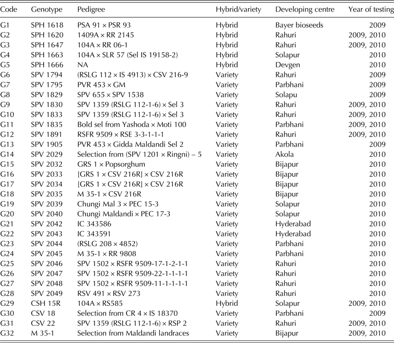
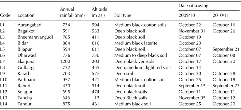
The data set used in the present study represent AICSIP data for 2009/10 and 2010/11 for post-rainy grain sorghum. In 2009/10, a set of 15 genotypes (four hybrids and 11 varieties) were evaluated across 14 locations, while in 2010/11, a set of 26 genotypes (five hybrids and 21 varieties) were evaluated across 11 locations. In addition, one variety with local adaptation was grown along with the test genotypes, treated as a local control (LC). Since the LCs varied from location to location they will not be discussed in subsequent sections. Nine genotypes were common in both years over locations. Detailed pedigree information about the genotypes is given in Table 1 and geographical positions of the test locations are shown in Fig. 1. The features and dates of sowing in the test locations are given in Table 2. The test locations were distributed among four states (Maharashtra – 6; Karnataka – 6; Telangana – 1; Gujarat – 1) that grow post-rainy sorghum in India. The crop was sown as the monsoons retreated, in September–October (Table 2). The experiments were laid out as alpha designs with three replications across all locations during the post-rainy seasons (September–March) of 2009/10 and 2010/11. Each year the experiments were planted in a plot with six rows each of 6 m length with 45 cm between rows and 15 cm between plants. Standard crop management practices were followed uniformly across all locations. For estimation of grain yield, the internal four rows were used and the panicles were harvested at physiological maturity. Plot yields for grain (dry matter basis) were converted to kg/ha using the plot size as factor.
Geographical position of test locations (L) and mega-environment (ME) pattern.

Information on the genotypes used in the study

NA, not available.
Information on the testing location

Data analysis
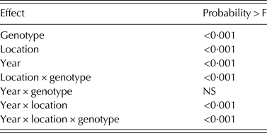
The combined data were analysed using PROC MIXED of SAS (version 9·3), in which block within replication and replication within location were kept as random effects. Fixed effect terms along with P-values are given in Table 3. The detailed statistical theories of AMMI and GGE methodology are elaborated in published literature (Zobel et al. Reference Zobel, Wright and Gauch1988; Yan & Kang Reference Yan and Kang2003). Since the data were unbalanced, a separate AMMI analysis of grain yield was carried out for 2009/10 and 2010/11 data using CropStat for Windows 7.2.2007·3. An AMMI stability value (ASV) of each genotype was calculated as described by Purchase et al. (Reference Purchase, Hatting and van Deventer2000). The following formula was used to calculate ASV for each genotype:
P-values for fixed effects of combined analysis

NS: Not significant.
where IPCA is interaction principal component axes, IPCA1ss/IPCA2
SS
is the weight derived from dividing the sum
 $ASV = \sqrt {{{[(IPC{1_{SS}}/IPC{2_{SS}}) \times (IPC{1_{score}})]}^2} + {{(IPCA{2_{score}})}^2}}$
of IPCA1 squares by the sum of IPCA2 squares.
Smaller ASV scores indicate a more stable genotype across environments. Software for GGE biplots does not accommodate alpha experimental designs. Hence, genotype × location two-way mean tables for each year were used as input data. Environment-centred matrices were calculated by subjecting the data to singular value decomposition (SVD). Tester-centred (centring 2) (s.d.-scaled, in which each value is divided by the standard deviation of its corresponding tester) and h-weighted (Scaling 2) GGE biplots were generated using GGE biplot software version 6·3 (Yan Reference Yan2001). Genotype evaluation was carried out using genotype-focused singular value partitioning (SVP = 1) and the ‘Mean v. stability’ option of GGE Biplot software. Reliability of the biplot was determined by the percentage of sum of squares (SS) explained by each principal component (PC), and the information ratios (IR) of each PC, which were obtained from the log file of the GGE output. The IR of a PC is the percentage of the total SS explained by the PC divided by the mean percentage of the PCs (Yan Reference Yan2014). Absolute values of the instability scores as obtained in the analysis were used for comparing the genotypes. Specific adaptation of the genotypes and ME were identified using the ‘Which-won-where’ option, to identify which genotype was the winner in a given set of locations. During combined analysis, the missing values were imputed by four cycles of SVD in-built in GGE software. Pearson's correlation between ASVs and GGE instability indices and the ranks of genotypes based on these values was calculated using the PROC CORR command of SAS (version 3.9).
RESULTS
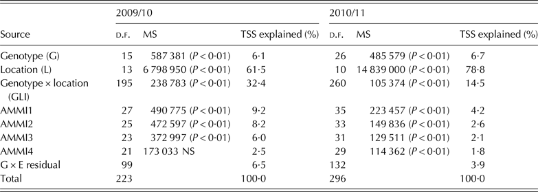
Genotype, location and year effects, and all their interactions except year × genotype were significant (Table 3). By analysing each year data using ANOVA, the yield SS were partitioned into genotype (G), location (L) and genotype × location interaction (GLI), which were highly significant (Table 4). In both years, L explained the highest percentage of total SS (61·5% in 2009/10 and 78·8% in 2010/11), which was followed by GLI (32·4% in 2009/10 and 14·5% in 2010/11) and the main effect of G (6·1% in 2009/10 and 6·7% in 2010/11, less than half of GLI). The GLI component was further partitioned by PCA: in 2009/10, the first two PCA axes explained 53·8% of interaction SS, while in 2010/11 the combined value was 46·5%. In 2009/10, first three PCs were significant, while in 2010/11 four PCAs were highly significant.
AMMI Analysis of grain yield of post-rainy sorghum in 2009/10 and 2010/11

d.f., Degrees of freedom; MS, Mean sum of square, TSS: Total sum of square.
The mean grain yield of genotypes in each location is presented in Table 5. In 2009/10, the grain yield ranged from 961 kg/ha (G32 at L7: see Tables 1 and 2 for genotype (G) and location (L) codes, respectively) to 4864 kg/ha (G3 at L9) with an average of 2372 kg/ha across locations. The highest-yielding genotype was G2, with an average yield of 2831 kg/ha, while the lowest-yielding was G30 (2021 kg/ha). Location mean yield ranged from 1367 kg/ha (L7) to 3325 kg/ha (L6). The average yield of the 2010/11 trial was 1920 kg/ha with G2 giving the highest average yield (2330 kg/ha) and L9 as location with the highest average yield (3458 kg/ha).

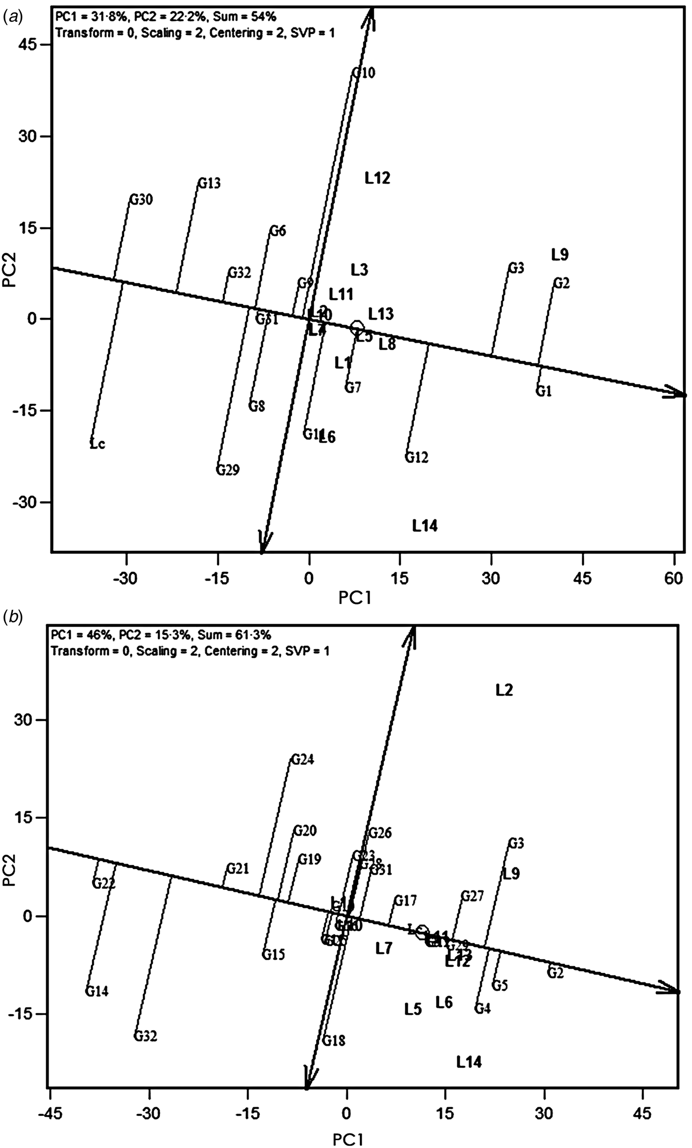
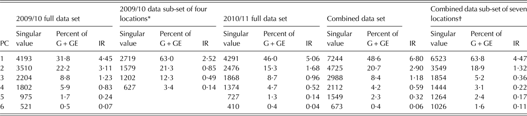
The ASV were calculated for each genotype. The lowest ASV in 2009/10 was recorded for G32 (4·27) followed by G31 (4·72) (Table 4). Other genotypes with low ASVs were G9, G6, G8 and G30. On the other hand, the highest ASV (34·56) was recorded for G10 followed by G1 (29·75) and G29 (26·96). Two-way genotype × location mean tables for each year were used as input for GGE analysis. The first two PCs in 2009/10 and 2010/11 explained 54·0 and 61·3% of the total variation, respectively (Table 6). The reliability of PCs was confirmed by the IR of each PC. In 2009/10, the first three PCs showed IR values >1·0, while in 2010/11, only the first two PCs had IR values >1·0. Performance and stability of genotypes were visualized graphically in GGE biplots using the average environment coordination (AEC) method (Fig. 2(a)). In environment-centred (centring = 2) genotype-metric (SVP = 1) biplots, the projection of a genotype over AEC abscissa (line with single arrow in Fig. 2(a)) indicates average yield, while the dispersion of a genotype along the AEC ordinate (double arrow in Fig. 2(a)) indicates its stability (Yan & Tinker Reference Yan and Tinker2006). The larger is the projection of a genotype along the AEC ordinate, the lower is its stability. In 2009/10 across locations, G1 and G2 followed by G3 and G12 were the highest-yielding genotypes. In contrast, G30, G13 and G32 were poor yielders. The observed ranking of genotypes is in close agreement with the mean yields of each genotype (Table 5). In 2010/11, the higher-yielding genotypes were G2, G5, G3 and G4 (Fig. 2(b)). On the other hand, G22, G14, G32 and G21 were poor performers for grain yield (Fig. 2(b)). Out of the highest-yielding genotypes in 2009/10, G1 was relatively stable with lower projection along the AEC ordinate, while other high yielders were relatively unstable. Genotype G10, followed by G29, with the longest projection along the AEC ordinate, indicated that it was most unstable and the corresponding ASVs of these cultivars were also very high (Table 5). In 2010/11, G29, G10, G12 and G9 had low GGE instability values, while G32, G24, G14, G18 and G3 recorded higher values. The lines identified as stable in GGE analysis mostly had low ASVs (Table 5). Similarly, the lines with higher instability values recorded higher ASVs. The GGE instability values and ASVs showed high correlation (r = 0·71, P < 0·01 in 2009/10 and r = 0·80, P < 0·001 in 2010/11). However, the rank correlations were lower, though still significant (r = 0·64, P < 0·01 in both years).


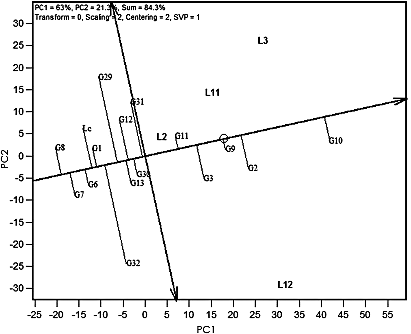
‘Which-won-where analysis’ of 2009/10 showed that most of the environments, except L6, L9, L12 and L14, were close to the origin of the biplot (non-discriminatory) and were highly correlated, while locations with higher location vector length (i.e. being away from the origin of biplot) were discriminatory (Fig. 3(a)). The biplot was divided into seven sectors, four accommodating all the 14 locations. The locations were partitioned into four groups. Group I was represented by L2, L3, L11 and L12 with G10 as the nominal winner; Group II represented L9, L10 and L13 with G2 and G3 as the winning genotype; Group III included L1, L4, L5, L7, L8 and L14 where G1 and G12 were the nominal winners. Group IV was solely represented by L6, without any distinct winning genotype. In order to confirm whether the GGE biplot of 2009/10 considering the first two PCs alone was reasonable enough to comprehend the trend in data, fresh biplots were generated using the sub-set of data representing the grouping of locations. Figure 3(a) shows that the group 1 environment was represented by L2, L3, L11 and L12 with G10 as the nominal winner. A sub-set of data with these locations alone generated a GGE biplot with G10 as distinct top performer with the first two PCs, explaining 84·3% of total SS and only the first PC to be informative with IR of 2·52 (Fig. 4). Almost similar correspondence could also be ascertained in other location groups with only one informative PC alone (data not shown).


‘Which-won-where’ analysis of 2010/11 data again suggested a closer relationship among the test locations, barring L2 with L14, L5 and L6 (Fig. 3(b)). Locations L1, L7 and L10 were non-discriminatory, being clustered at the origin of the biplot. The biplot was partitioned into eight sectors, of which four retained all the 11 locations. The major group (I) was represented by L5, L6, L7, L9, L11, L12, L13 and L14, having three winners (G2, G5 and G4). The other three groups (II, III, IV) were represented by single locations, viz., L2 with G3 as winner; L1 with G22 as nominal winner; and L10 with winning genotype G14.
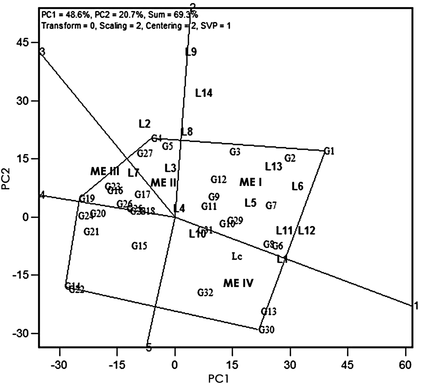
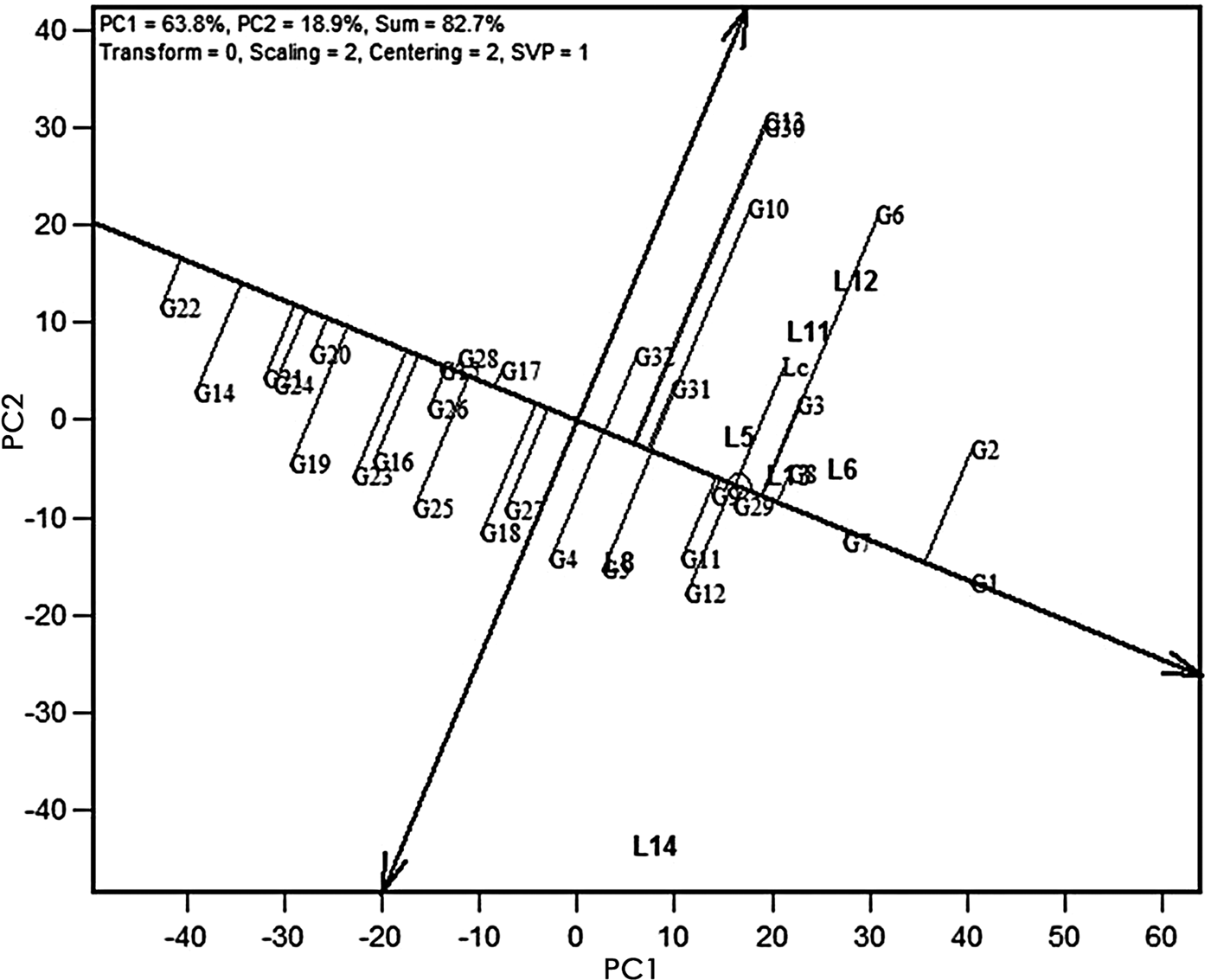
Towards the identification of ME, combined GGE analysis of genotype × location mean tables for the 2 years were subjected to four cycles of SVD to estimate the missing values. The GGE analysis gave rise to three PCs having IR > 1·0 (Table 6). The first two PCs explained 69·3% of total SS. The biplot was partitioned into five sectors, out of which four sectors contained all locations, suggesting the existence of four possible ME (Fig. 5). The major ME, ME I, was represented by L5, L6, L8, L11, L12, L13 and L14 with G1 followed by G2 as nominal winners. The second ME comprised L2, L3, L4 and L9 with G4 followed by G5 as nominal winning genotypes, while ME III and IV represented two small ME. A single location, L7, with G19 as winner genotype was seen for ME III, while ME IV consisted of locations L1 and L10, with G30 followed by G13 as winners. To test the reliability of the pattern revealed in Fig. 5, as explained earlier, fresh biplots were generated using a sub-set of the original data with the groups identified. For example, a new biplot with the locations of Group 1 of Fig. 5 showed very clearly that G1 followed by G2 were the best performers in this group of locations (Fig. 6). The first two PCs, which were only informative with IR values >1·0, explained 82·7% of total SS. The near-perfect match of winners in other groups of locations as obtained in Fig. 5 matched in the sub-set biplots as well (data not shown). Hence, it can be said that Fig. 5 is a succinct summary of the data in the combined data set.


DISCUSSION
Post-rainy season sorghum is consumed as food in India, and its cultivation is concentrated in the dry tracts of inland Central and Eastern Maharashtra and inland Northern Karnataka states of India. In the present work, the GEI among the AICSIP post-rainy sorghum testing locations and genotypes was studied for 2 years, 2009/10 and 2010/11. In 2009/10, a set of 15 genotypes along with LCs were evaluated over 14 locations, while in 2010/11, a total of 26 genotypes and a LC were evaluated across 11 locations. Nine genotypes and 11 locations were common in both seasons. Year, location, genotype and their interactions, except year × genotype, indicated the presence of considerable variability in the data and existence of significant interaction, and calls for focused study to understand them. Year-wise AMMI analysis indicated that location is the highest contributor towards total variation followed by GLI and genotype. Up to 80% contribution of environment towards overall variation in MLT data has been reported in many crops (Gauch & Zobel Reference Gauch and Zobel1997; Dehghani et al. Reference Dehghani, Ebadi and Yousefi2006; Tolessa et al. Reference Tolessa, Keneni, Sefera, Jarso and Bekele2013). In the present study, the contribution of location was higher and that of GLI lower in 2010/11 as compared with 2009/10. The observed variation due to GLI effect in the present study was close to that reported in sorghum (Rakshit et al. Reference Rakshit, Ganapathy, Gomashe, Rathore, Ghorade, Nagesh Kumar, Ganesmurthy, Jain, Kamtar, Sachan, Ambekar, Ranwa, Kanawade, Balusamy, Kadam, Sarkar, Tonapi and Patil2012a ), wheat (Koutis et al. Reference Koutis, Mavromatis, Baxevanos and Koutsika-Sotiriou2012) and rice (Samonte et al. Reference Samonte, Wilson, McClung and Medley2005), but higher than barley (Dehghani et al. Reference Dehghani, Ebadi and Yousefi2006). The GLI explained two (in 2010/11) to six (in 2009/10) times higher proportion of the variation than G, which indicated the possible existence of ME among test locations (Rakshit et al. Reference Rakshit, Ganapathy, Gomashe, Rathore, Ghorade, Nagesh Kumar, Ganesmurthy, Jain, Kamtar, Sachan, Ambekar, Ranwa, Kanawade, Balusamy, Kadam, Sarkar, Tonapi and Patil2012a ).
In the AMMI model, G is separated from GE: G is considered to depict the general adaptation, while GE represents specific adaptation (Zobel et al. Reference Zobel, Wright and Gauch1988). Contrary to this, G is assumed to represent the general adaptation in GGE analysis, whereas the specific adaptation is a combined effect of G + GE (Yan Reference Yan2014). In GGE biplot analysis, complex GEIs are partitioned into different PCs and the data are presented graphically against various PCs (Yan & Tinker Reference Yan and Tinker2006). The AMMI model lacks a direct quantitative stability measure, which can quantify and rank genotypes according to their yield stability. To address this, Purchase et al. (Reference Purchase, Hatting and van Deventer2000) proposed a quantitative measurement of stability using AMMI scores of genotypes as ASVs (ASV is the distance from zero in a two-dimensional scatter plot of IPCA1 scores against IPCA2 scores). Farshadfar et al. (Reference Farshadfar, Mahmodi and Yaghotipoor2011) explained that ‘since the IPCA1 score contributes more to GE SS, it has to be weighted by the proportional difference between IPCA1 and IPCA2 scores to compensate for the relative contribution of IPCA1 and IPCA2 total GE SS’. Subsequently, the distance from zero is determined using the theorem of Pythagoras (Purchase et al. Reference Purchase, Hatting and van Deventer2000). On the contrary, the stability of genotype is estimated by the projection of a genotype onto the average environment axis (AEA) ordinate in the GGE biplot. Less stable genotypes are projected higher on the AEA ordinate (Yan Reference Yan2001; Yan & Tinker Reference Yan and Tinker2006). In the present study, the stability of genotypes was determined by both ASVs and GGE instability scores, and they showed high correlation in both years. However, large deviations were observed in isolated cases in terms of the ranking of genotypes following both indices. As observed, G1 ranked 14th for ASV (29·75), but the GGE biplot depicted it as a stable genotype. Regression analysis revealed that out of the 15 cultivars tested in 2009/10, the slopes of only G2 and G3 deviated significantly from unity (1·516 and 1·426, respectively), indicating their instability. Though G1 was found to be unstable in AMMI analysis, GGE and regression analyses revealed that it should not be rejected as unstable and may be retained since it is second to G2 in terms of mean grain yield. Similarly, in 2010/11, G9 ranked 16th in terms of its ASV score but fifth according to GGE instability score. However, it may be noted that the ASV for this genotype was not very high (13·77) though it ranked 16th. Since it is not among the top ranking genotypes, the change in rank actually does not interfere with the conclusions. Thus, both AMMI and GGE analyses gave rise to very similar conclusions in terms of the identification of best-performing genotypes. By employing GGE biplots alone, several authors have identified high-performing and stable genotypes in different crop species including barley (Dehghani et al. Reference Dehghani, Ebadi and Yousefi2006; Mortazavian et al. Reference Mortazavian, Nikkhah, Hassani, Sharif-Al-Hosseini, Taheri and Mahlooji2014), wheat (Koutis et al. Reference Koutis, Mavromatis, Baxevanos and Koutsika-Sotiriou2012), sorghum (Rakshit et al. Reference Rakshit, Ganapathy, Gomashe, Rathore, Ghorade, Nagesh Kumar, Ganesmurthy, Jain, Kamtar, Sachan, Ambekar, Ranwa, Kanawade, Balusamy, Kadam, Sarkar, Tonapi and Patil2012a ) and others (Sabaghnia et al. Reference Sabaghnia, Dehghani and Sabaghpour2008; Tolessa et al. Reference Tolessa, Keneni, Sefera, Jarso and Bekele2013).
In GGE biplots, projections of genotypes on to the AEC abscissa approximate their average yield (Yan & Tinker Reference Yan and Tinker2006). In the present study, the ranking of genotypes for average yield based on GGE biplots and that of actual data are in close agreement. It is observed that though the sum total of the first two PCs in 2009/10 and 2010/11 were 54·0 and 61·3%, respectively; the inherent pattern in the data both for means and stability is represented realistically in the GGE biplot as well as AMMI analysis. To determine how good was the fit in GGE analysis, IR values of respective PCs were checked. Yan (Reference Yan2014) suggested that a PC with IR value >1·0 is informative, while PCs with <1·0 are not and may therefore be rejected. It was found that in 2009/10, though the first three PCs had IR values >1·0, the first PCs together could summarize the data trend effectively. Analysis of sub-set data (Fig. 4) clearly showed that the relation revealed in Fig. 3(a) is true representation of the data trend. The observed trend in terms of top performance of the genotype in a given location could be derived from a means table too, particularly for locations which were highly discriminating. Locations with higher distance from the origin of the biplot have a longer location vector and are highly discriminating, while the locations closer to the origin are non-discriminatory. Disparity of the grouping based on the GGE biplot and the mean table was observed among non-discriminatory locations.
Angles between the location vectors in GGE biplots indicate their relationships because the cosine of the angle between two vectors is indicative of their correlation (Yan & Tinker Reference Yan and Tinker2006). An acute angle between two environment vectors is indicative of positive correlation, while an obtuse angle indicates negative correlation and a right angle suggests no correlation (r = ~0). In both years (particularly in 2009/10), it was found that a majority of locations were closely related, which has also been observed in other sorghum MLT data (Rakshit et al. Reference Rakshit, Ganapathy, Gomashe, Rathore, Ghorade, Nagesh Kumar, Ganesmurthy, Jain, Kamtar, Sachan, Ambekar, Ranwa, Kanawade, Balusamy, Kadam, Sarkar, Tonapi and Patil2012a , Reference Rakshit, Ganapathy, Gomashe, Swapna, More, Gadakh, Ghorade, Kajjidoni, Solanki, Biradar and Prabhakar2014). Non-discriminating and closely related locations may be dropped in future from the programme as they will not generate any additional information. Hence, as suggested by Rakshit et al. (Reference Rakshit, Ganapathy, Gomashe, Rathore, Ghorade, Nagesh Kumar, Ganesmurthy, Jain, Kamtar, Sachan, Ambekar, Ranwa, Kanawade, Balusamy, Kadam, Sarkar, Tonapi and Patil2012a ), similar environments could be removed from MLT of sorghum genotypes, which would help in optimal utilization of limited resources during trial allocations. Results of both years showed few locations having obtuse angles, suggesting the existence of strong cross-over interaction in the data (Yan & Tinker Reference Yan and Tinker2006). It can be noted that both crossover and non-crossover interactions were present in the data. The observed mixture of crossover and non-crossover types of GEI in MLT is of very common occurrence (Sabaghnia et al. Reference Sabaghnia, Dehghani and Sabaghpour2008; Rao et al. Reference Rao, Reddy, Rathore, Reddy and Panwar2011; Rakshit et al. Reference Rakshit, Ganapathy, Gomashe, Rathore, Ghorade, Nagesh Kumar, Ganesmurthy, Jain, Kamtar, Sachan, Ambekar, Ranwa, Kanawade, Balusamy, Kadam, Sarkar, Tonapi and Patil2012a ). Higher response of selected genotypes to change in the growing environment may lead to this phenomenon as response to environment is a combined property of gene combinations they carry.
The ‘Which-won-where’ view is the most attractive feature of the GGE biplot, which graphically addresses crossover GEI, mega-environment differentiation and specific adaptation (Yan et al. Reference Yan, Hunt, Sheng and Szlavnics2000; Yan & Tinker Reference Yan and Tinker2006; Rao et al. Reference Rao, Reddy, Rathore, Reddy and Panwar2011; Rakshit et al. Reference Rakshit, Ganapathy, Gomashe, Rathore, Ghorade, Nagesh Kumar, Ganesmurthy, Jain, Kamtar, Sachan, Ambekar, Ranwa, Kanawade, Balusamy, Kadam, Sarkar, Tonapi and Patil2012a ). Such a biplot summarizes the complex GEI pattern of MLT data in a concise way. Projection of the biplot using PC1 and PC2, explaining 69·3% of variation, brought out two major MEs and two additional minor MEs (Fig. 5). In this analysis, three PCs recorded an IR score of >1·0 (Table 6). Reliability of the pattern revealed in Fig. 5 was tested by creating a biplot using a sub-set of the original data with the groups identified (Fig. 6). It was found that though three PCs had IR > 1·0 the biplot with first two PCs could summarize the trend effectively.
The present study found that a major ME (ME1) was represented by seven locations, viz., L5, L6, L8, L11, L12, L13 and L14. Geographically they are distributed across four states, i.e. Karnataka, Maharashtra, Telangana and Gujarat. Though geographically all the locations are spread wide apart, they are characterized by relatively deeper soil and crop grown under conserved moisture. A second ME was represented by L2, L3, L4 and L9. All these locations are of geographical proximity, with the first three locations situated in Northern Karnataka and L9 in Southern Maharashtra. The soils of these locations are medium to deep Alfisols and have low rainfall. A third ME was represented by L1 and L10, located in the Marathwada region of Maharashtra, having low rainfall and medium Vertisols. The fourth ME with L7 is located in the Vidharbha region of Maharashtra, characterized by high rainfall and deep Vertisols. Unlike Rakshit et al. (Reference Rakshit, Ganapathy, Gomashe, Rathore, Ghorade, Nagesh Kumar, Ganesmurthy, Jain, Kamtar, Sachan, Ambekar, Ranwa, Kanawade, Balusamy, Kadam, Sarkar, Tonapi and Patil2012a ), who did not find much correlation between ME and physio-climatic characteristics of the locations, the present study could broadly explain the grouping of environments by soil type, rainfall pattern and prevalence of moisture conservation practices. It may be noted that a similar conclusion is drawn from the locations within same ME. Hence, non-discriminating locations (with smaller location vector) may be dropped within an ME to reduce the cost of trial execution. For example, the main ME identified in the present study has almost all seven locations being discriminatory, but L4 is not very discriminatory within the second ME, and hence may be dropped. However, this pattern needs to be reconfirmed using data from more years, as carried out in wheat (Yan et al. Reference Yan, Hunt, Sheng and Szlavnics2000) and peanut (Casanoves et al. Reference Casanoves, Baldessari and Balzarini2005; Putto et al. Reference Putto, Patanothai, Jogloy and Hoogenboom2008). Existence of high crossover GEI in the post-rainy season data and occurrence of MEs within test locations clearly indicates the need to breed for location-specific cultivars, rather than expecting to obtain cultivars with wider adaptation across all locations. The existing methods of promotion and identification of new cultivars based on ‘across location means’ may not be sufficient to actually judge the potentiality of cultivars in question. Even if such analyses are carried out, the criteria in the promotion and identification process must also include stability parameters.
CONCLUSION
The present study demonstrated the utility and convenience of GGE biplot analysis on a par with AMMI analysis in the identification of stable genotypes with higher grain yield and visualization of mixed crossover effects (complex GEI). The study also showed the location-specific adaptation of genotypes. Hence, sorghum breeders across the world need to focus on the requirement of specific adaptation, rather than expecting to breed genotypes with wider adaptability. Breeding priorities need a shift from the existing station-oriented research to participatory plant breeding. Existence of ME, as identified through ‘Which-won-where’ analysis, indicated that the non-discriminating locations within MEs can be dropped. This will enable an effective allocation of available resources. High cross-over GEI clearly indicated that the present procedure of varietal release that considers means of yields across locations may not be the best strategy. Actual stability of the genotype needs to be reflected in the cultivar release process.
Help from Dr P. Rajendra Kumar in editing the manuscript is gratefully acknowledged. The authors also thank KV Kumar of ICAR-National Academy of Agricultural Research Management for locating the test locations on the map.