THE MODEL

Our multi-level prediction builds on our successful model predicting the House seat division in 2006 (Bafumi et al. Reference Bafumi, Erikson, Wlezien, Alvey and Scheuren2008).Footnote ¹ The model has two steps. Step 1 predicts the midterm vote division from only two variables, the generic poll result and the party of the president. With this measure of the partisan tide in place, step 2 forecasts the winners of 435 House races using separate statistical models for open seats and races with incumbent candidates. At each step, the forecast takes into account uncertainty about the inputs. The final product is a prediction of the partisan division of House seats, as well as a probabilistic statement regarding the likelihood of the Republican Party regaining control of the chamber.

STEP 1: PREDICTING THE VOTE

Our prediction of the national division of the two-party vote is based on two independent variables. One variable is the recent reading of the generic polls—the frequently asked poll question regarding preferences on a generic (no candidate names) partisan ballot for Congress.Footnote ² The second variable is a dummy variable for the party holding the presidency. We have modeled this process in detail elsewhere (Bafumi et al. Reference Bafumi, Erikson and Wlezien2010). In past congressional campaigns, generic polls have persistently underestimated the ultimate support for the non-presidential (“out”) party. This tendency is greatest early in the election year and recedes as the campaign progresses. Poll respondents increasingly take into account the party of the president when reporting their generic vote. As the campaign progresses, they tilt toward the out-party. Our interpretation (Bafumi et al. Reference Bafumi, Erikson and Wlezien2010) is that voters seek more ideological balance between the president and Congress.

Remarkably, forecasts from our two variables—the generic poll results and the party of the president—are about equally predictive regardless of when the poll results are taken. In short, the midterm vote tends to be determined early, with the campaign serving mainly to draw the voters toward the out-party. Taking into account election-year changes in the president's approval rating or economic conditions has not offered any improvements to the forecast equation in the past (Bafumi et al. Reference Bafumi, Erikson and Wlezien2010). Our two variables predict the November vote approximately as well as final presidential trial-heat polls predict the presidential vote (see Wlezien and Erikson Reference Wlezien and Erikson2002).

For our forecast, we measure the Democratic percent of the two-party vote (minus 50%) in reported generic ballot polls conducted by personal interview (no robotic or Internet polls).Footnote ³ A slight adjustment is necessary to combine polls from different target populations—specifically, adults, registered-voter, and likely-voter polls. Reflecting the historical tendency for adult and registered-voter polls to favor Democrats more than likely-voter polls, we subtract 1.85 percentage points from the Democratic margin for polls of adults and 1.04 percentage points for registered-voter polls, thereby norming the measure, as with likely-voter samples.Footnote ⁴ With this adjustment and the generic polls measured 121 to 180 days in advance of the election (centered in early June), the vote forecasting equation for the 16 midterm elections between 1946 and 2006 isFootnote ⁵:

(1)

where (to aid interpretation) the vote and poll variables are measured as deviations from 50%, and PresParty = 1 if a Democratic president and −1 if a Republican president. Both independent variables are statistically significant at the .001 level; the intercept is not significant. The adjusted R ² for the equation is 0.73, and the root mean squared error (RMSE) is 1.94.

The pooled generic polls conducted 121 to 180 days in advance of the 2010 election show a very close division of 49.1% Democratic and 50.9% Republican.Footnote ⁶ But a virtual tie in the polls at this point projects a significant vote plurality for the Republicans as the out-party. This predicted outcome is not due to any bias in the polls, but rather stems from the electorate's tendency to gravitate further toward the “out” party over the midterm year—ultimately gaining about two extra points beyond what the June polls would otherwise show.

Our specific forecast is that the Democrats will win 47.1% of the two-party vote and the Republicans the remaining 52.9%. We take into account the uncertainty about this forecast by simulating 1,000 cases based on the forecast error associated with our prediction for 2010.Footnote ⁷ This model yields a probability density as a distribution around the forecast. By this estimate, the 95% confidence band is a range from 43.1% to 51.1% Democratic. The Republicans win the popular vote 91% of the time.

STEP 2: PREDICTING SEATS

The national vote only tells us part of the story, and we still need to determine how it would translate into seats. For each simulated value of the national vote, we need to simulate the outcome in 435 congressional districts. The district vote (D _jk) is a function of the stochastic simulations of the national vote (simulation j) and the local conditions (simulation k):

where L _k = the expected local component of the vote in the kth district and u _k = the simulation of the district k error. The national vote in the jth simulation (N _j) consists of the specific prediction (P) from equation 1 plus the error (e _j) around that prediction. Substituting in these components yields:

The formula for L _k differs for open seats and incumbent races. For open seats (no incumbent running), the district vote simulation comes from equation 2:

(2)

where Obama%_k = the Obama percentage of the two-party vote in district k in 2008. D _jk and Obama% are calibrated as deviations from 50%. For seats of districts where the incumbent seeks reelection, the district vote simulation comes from equation 3:

(3)

where Dem Vote (2008)_k = the Democratic vote percentage for the House in district k in 2008 (minus 50%) and Frosh_k = 1 if a freshman Democrat in 2010, −1 if a 2010 freshman Republican, and 0 otherwise.

The numerical parameters of equations 2 and 3 are derived from regression equations predicting (1) the 2008 district vote for 2008 open seats with the presidential vote in that district, and (2) 2008 incumbent races with the 2006 district-level vote for the incumbent plus the freshman indicator.Footnote ⁸ Recalling that all vote variables are calibrated as deviations from 50% Democratic, the two constant terms represent the expected vote when the partisan trend plus the Obama district vote or the lagged incumbent district vote equal 50% Democratic. For equation 2, the constant term equals the intercept for the 2008 open-seat equation minus the 2008 national vote for Democrats. For equation 3, the constant term is set to the value at which, given any value of the national vote, the projected average change from 2008 to 2010 in the mean district vote equals the projected 2008–10 change in the national vote.

Importantly, the RMSEs from the two 2008 regression equations provide the standard deviations for u _{k_open} and u _{k_incumbent}. For open seats, this value is 6.86. For incumbent races, it is 4.91. These values represent the uncertainty around the district vote after taking into account the projected district vote from the 2008 presidential vote (open seats) or 2008 congressional vote (incumbent seats). For vote estimates drawn from P + e _j, we simulate the winner in each district. We conducted 1,000 simulations to take into account the variability characterized by the associated error terms, e _j and u _{k_open} or u _{k_incumbent}.

FORECASTING 2010

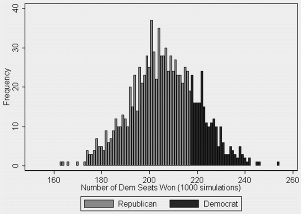
First, we generated 1,000 simulations of the national vote based on equation 1. Then, we applied each of the 1,000 simulated national outcomes to each congressional district, using the formulas shown in equations 2 and 3, predicting the likelihood of a Democratic victory in each. For each of the 1,000 simulated vote outcomes, we arrived at a projected outcome in terms of the partisan division of 435 congressional districts. Figure 1 displays the resulting density of results. As can be seen from the predominance of gray bars, the Republicans win the majority of seats in 79% of the trials. On average, the Republicans win 229 seats, 23 more than the Democrats and 11 more than the 218 needed for a majority. However, the simulations yield considerable variation, with a 95% confidence interval of 176 to 236.Footnote ⁹

Figure 1

One Thousand Simulations of the 2010 Election

Note that the Democrats' chance of holding the House (21%) is greater than the chance of the Democrats winning the popular vote (9%). This apparent discrepancy arises because the critical value of the popular vote at which the identity of the majority party becomes a 50-50 proposition is 48.8%. The Democrats need not win the majority of the vote to win the most seats. The fact that popular Democratic incumbents currently hold many of the seats that would normally be competitive provides the Democrats with a partial barrier against a Republican deluge.

A NOTE OF CAUTION

Applying our model of the vote to 2010 assumes that the forces at work in 2010 are unchanged from past midterm elections. However, we should be wary of the possibility that the underlying model of the national vote works differently in 2010 or is influenced by variables we have not taken into account. In particular, we note that in past elections, the out-party usually has increased its support in the generic polls as the election year campaign has progressed. But this increase did not happen in the first six months of 2010. The generic polls have hovered around a 50-50 division rather than sliding further in the Republicans' favor, which may reflect a strong public engagement in the campaign far earlier than has occurred in the run-up to previous midterms. From the start, the 2010 campaign has had a sharper ideological tone than in the past. The tilting toward the out-party may thus have been realized earlier than in the past.Footnote ¹⁰ It also is possible that an unusually conservative Republican campaign could dampen the expected shift toward the Republicans. If either of these possibilities is true and the polls remain unchanged through November, the Democrats actually could have the edge come Election Day.

FORECASTING FROM OCTOBER POLLS

From the perspective of the reader in October of 2010, forecasts based on late polls from October are more valuable than from July, our publication deadline. As an aid to predict the outcome late in the campaign, we present the vote forecasting equation based on generic polls during the final 30 days of past campaigns in the 16 midterm elections between 1946 and 2006:

(4)

where the vote and poll variables are measured as deviations from 50%, and PresParty = 1 if a Democratic president and −1 if a Republican president.Footnote ¹¹

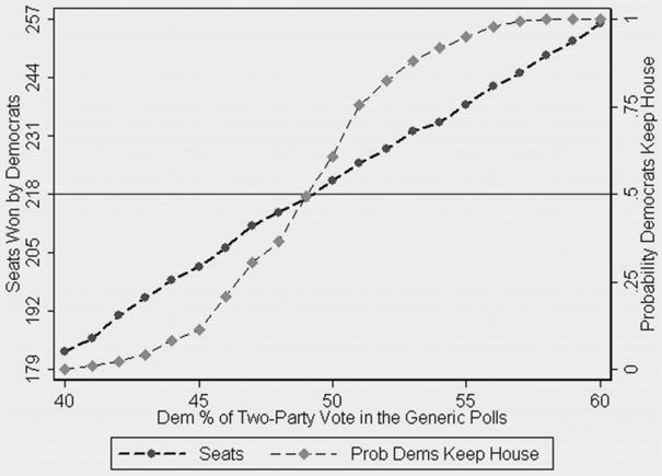
The key difference between equation 4 and equation 1 is that the penalty for belonging to the presidential party is much lower in October, declining from almost two points to less than one point. Should the generic polls stay close to 50-50, as they were through early July, prospects will look much better for the Democrats. At 121 to 180 days out, the Democratic share in the generic polls was 49.1%. A continuation at this value into October would project the Democrats winning 48.8% of the actual national vote and having an even (50%) chance of retaining the House.

As a guide, we have estimated both the expected seat outcome and the probability of Democratic control, given a continuum of scenarios regarding the late generic polls. Figure 2 shows the results. The Democrats are favored to maintain control of the House as long as they win at least 49.2% of the two-party vote in October's (likely voter) generic polls, which converts to an expectation of 48.9% or more of the popular vote. Should they hold a 50% poll share at the end of the campaign, the Democrats will have a 63% chance to retain the House.

Figure 2

Simulations of the 2010 Election Outcome, Conditional on the Generic Polls in the Final 30 Days before the Election