

1. Introduction
The causes of mass extinctions have been debated for over two centuries. They have been reviewed in innumerable papers and books, including those authored by the honorand of this volume (e.g. Hallam & Wignall, Reference Hallam and Wignall1997; Hallam, Reference Hallam2005). Extinctions are a modern zeitgeist, with existential threats from global warming, meteorite impacts, pandemics and nuclear war, but they have been important in the evolution of life and, to geologists, by providing important marker horizons throughout the Phanerozoic Eon. They also have the potential to inform about the effects of current and predicted climate change.
There is a growing consensus that mass extinctions are a consequence of catastrophic and rapid changes in the Earth-surface carbon cycle (ESCC). These changes cannot be easily explained by processes that operate on a geologically long timescale (e.g. sea-level rise or fall, plate movement leading to formation of mountain belts or blocking of ocean circulation systems), so attention has turned to more dramatic triggers such as meteorite or comet impacts, flood basalts eruptions and extra-solar events such as gamma-ray bursts (Thomas et al. Reference Thomas, Melott, Jackman, Laird, Medvedev, Stolarski, Gehrels, Cannizzo, Hogan and Ejzak2005). Whether or not gamma-ray bursts are a trigger mechanism is virtually untestable, but at least one impact event coincides with one mass extinction (Chicxulub and the end-Cretaceous mass extinction; Schulte et al. Reference Schulte, Alegret, Arenillas, Arz, Barton, Bown, Bralower, Christeson, Claeys, Cockell, Collins, Deutsch, Goldin, Goto, Grajales-Nishimura, Grieve, Gulick, Johnson, Kiessling, Koeberl, Kring, MacLeod, Matsui, Melosh, Montanari, Morgan, Neal, Nichols, Norris, Pierazzo, Ravizza, Rebolledo-Vieyra, Reimold, Robin, Salge, Speijer, Sweet, Urrutia-Fucugauchi, Vajda, Whalen and Willumsen2010).
Following the discovery of an iridium anomaly and other indicators of an extra-terrestrial input at the end-Cretaceous, Alvarez et al. (Reference Alvarez, Alvarez, Asaro and Michel1980) proposed that a meteorite impact caused the end-Cretaceous mass extinction. This arguably made decades of research into the causes of the extinction redundant virtually overnight, whilst simultaneously kick-starting searches for impact sites and the terrestrial effects of impactors. While the latter certainly occurred, the former turned out not to be true; alternative models refused to go extinct. In the aftermath of the Alvarez study, for example, several papers argued that the evidence for impact could also be explained by flood basalt volcanism (e.g. Officer & Drake, Reference Officer and Drake1983, Reference Officer and Drake1985; Officer et al. Reference Officer, Hallam, Drake and Devine1987). However, the discovery of the impact site in the Yucatan Peninsula and innumerable subsequent studies strengthened the case for an impact, at least for the end-Cretaceous extinction, and culminated in the ‘guilty as proven’ review of Schulte et al. (Reference Schulte, Alegret, Arenillas, Arz, Barton, Bown, Bralower, Christeson, Claeys, Cockell, Collins, Deutsch, Goldin, Goto, Grajales-Nishimura, Grieve, Gulick, Johnson, Kiessling, Koeberl, Kring, MacLeod, Matsui, Melosh, Montanari, Morgan, Neal, Nichols, Norris, Pierazzo, Ravizza, Rebolledo-Vieyra, Reimold, Robin, Salge, Speijer, Sweet, Urrutia-Fucugauchi, Vajda, Whalen and Willumsen2010).
Confirmation that meteorite or comet impacts caused other mass extinctions or dramatic changes to the ESCC has proved elusive (White & Saunders, Reference White and Saunders2005; Racki, Reference Racki2012), although they have been proposed for both the end-Permian (Becker et al. Reference Becker, Poreda, Hunt, Bunch and Rampino2001) and end-Paleocene (Kent et al. Reference Kent, Cramer, Lanci, Wang, Wright and Van der Voo2003) events. However, there has been a steady and growing argument that flood basalts (or the more embracing category of ‘large igneous provinces’, which include oceanic plateaus such as the Ontong Java Plateau) were the primary cause of many mass extinctions and other Earth-system crises, rather than meteorite impacts.
The term ‘flood basalt’ was introduced by Tyrrell (Reference Tyrrell1937), following the evocative description of Geikie (Reference Geikie1903): ‘. . .there have been periods in the earth's history when the crust was rent by innumerable fissures over areas of thousands of square miles in extent, and when the molten rock. . .welled out from these rents. . .and flooded enormous tracts of country without forming any mountain or conspicuous volcanic cone. . .’ Such events may rapidly pollute the Earth's surface via a number of processes. Vogt (Reference Vogt1972) was one of the first to associate flood basalts (and mantle plume activity) with mass extinction events, suggesting that the introduction of toxic concentrations of trace metals in the oceans was the ‘kill’ mechanism. McLean (Reference McLean1985), focusing on the effects of volcanic CO2, has been a strong advocate for the Deccan Traps as the cause of the end-Cretaceous mass extinction, even in the face of strong opposition. Other workers have emphasized the role of volcanic SO2 and sulphate aerosols in generating volcanic winters where surface temperatures would plummet for short intervals of time (Stothers et al. Reference Stothers, Wolff, Self and Rampino1986; Rampino, Self & Stothers, Reference Rampino, Self and Stothers1988; Saunders and Reichow, Reference Saunders and Reichow2009; Mussard et al. Reference Mussard, Le Hir, Fluteau, Lefebvre, Godderis, Keller and Kerr2014). Furthermore, the inventory and volume of volatiles released by the volcanic activity may be considerably enhanced by injection of sills into evaporates and organic-rich sediments (Svensen et al. Reference Svensen, Planke, Malthe-Sørenssen, Jamtveit, Myklebust, Eidem and Rey2004, Reference Svensen, Planke, Chevallier, Malthe-Sorenssen, Corfu and Jamtveit2007, Reference Svensen, Planke, Polozov, Schmidbauer, Corfu, Podladchikov and Jamtveit2009a ).
There is therefore no shortage of ‘kill mechanisms’ associated with large-scale volcanism (and indeed large meteorite or cometary impacts), but evidence for impacts at the time of most mass extinction events is unconvincing (see review by Racki, Reference Racki2012). Many mass extinction events and several oceanic anoxic events and hyperthermals, on the other hand, coincide with flood basalt eruptions. Given the geologically short duration of most flood basalt events, the likelihood of this being pure chance is very small (e.g. Rampino & Stothers, Reference Rampino, Self and Stothers1988; Stothers, Reference Stothers1993; Courtillot, Reference Courtillot1994; Wignall, Reference Wignall2001; Courtillot & McLinton, Reference Courtillot and McLinton2002; White & Saunders, Reference White and Saunders2005; Bond & Wignall, Reference Bond, Wignall, Keller and Kerr2014). It remains unclear, though, why some large igneous provinces (LIPs, e.g. Paraná-Etendeka) do not cause mass extinctions and why there is apparently such a poor correlation between volume of LIP and the severity of the mass extinction (Wignall Reference Wignall2001; Ganino & Arndt, Reference Ganino and Arndt2009; Bond & Wignall, Reference Bond, Wignall, Keller and Kerr2014), although this is not the case for the two systems reviewed here.
This review focuses on the relationships between two large igneous provinces and their associated environmental catastrophes. The North Atlantic igneous province (NAIP) developed during late Paleocene – early Eocene time and is contemporaneous with the Paleocene–Eocene thermal maximum (PETM) (Storey, Duncan & Swisher, Reference Storey, Duncan and Swisher2007), a major hyperthermal which is characterized by large and rapid shifts in global temperature and the carbon cycle, and accompanied by a significant mass extinction of benthic formaninfera. The Siberian Traps erupted around the time of the Permo-Triassic (P–Tr) boundary and were synchronous (Renne & Basu, Reference Renne and Basu1991; Campbell et al. Reference Campbell, Czamanske, Fedorenko, Hill and Stepanov1992; Reichow et al. Reference Reichow, Pringle, Al'Mukhamedov, Allen, Andreichev, Buslov, Davies, Fedoseev, Fitton, Inger, Medvedev, Mitchell, Puchkov, Safonova, Scott and Saunders2009) with the end-Permian mass extinction (EPME), the largest known, and also with a large and global change in the global carbon cycle and temperature. The two systems therefore show strong similarities: contemporaneous, large-volume basaltic volcanism and a mass extinction; and they both occurred during periods when the Earth was at least in warm-house conditions, with no permanent/major polar ice caps. Both systems show significant and rapid-onset changes to the ESCC. Global warming during both the PETM and EPME is clearly documented by oxygen isotope studies. Both volcanic provinces erupted at high latitude. Both the PETM and EPME are well documented by high-precision radiometric dating.
There are, however, some important differences. The NAIP is smaller (at least in terms of area) by up to a factor of 2 than the Siberian Traps. While the Siberian Traps are wholly continent-based, the NAIP was initially continental and later developed into an oceanic rift system. While significant, the extinction during the PETM affected only benthic fauna whereas the EPME was the largest known, exterminating >50% of genera in both marine and terrestrial environments. While both events saw extensive marine acidification, with a well-documented shallowing of the lysocline during the PETM (Zachos et al. Reference Zachos, Röhl, Schellenberg, Sluijs, Hodell, Kelly, Thomas, Nicola, Raffi, Lourens, McCarren and Kroon2005), the EPME also saw development of major marine anoxia and euxinia that lapped onto the continental shelves and may even have reached the surface (Wignall & Twitchett, Reference Wignall and Twitchett1996; Kump, Pavlov & Arthur, Reference Kump, Pavlov and Arthur2005). Anoxia during the PETM appears to have been much more limited in extent and intensity (Dickson, Cohen & Coe, Reference Dickson, Cohen and Coe2012; Pälicke, Delaney & Zachos, Reference Pälicke, Delaney and Zachos2014), although low oxygen levels in oceanic bottom waters may have been the cause of the extinction of benthic foraminifera (Thomas, Reference Thomas and Crame1989).
Can we determine the processes that were responsible for the similarities and differences between these two sets of major events? Recent high-precision age dates for both igneous provinces and their contemporaneous surface environment allow a detailed evaluation of the chronology and causes leading up to, and beyond, the two global catastrophes. Three important inputs are required to model any impact of LIPs on the Earth's climate system: (1) the total mass and (2) type of volatiles that are released, and (3) the rate at which they are released. To determine these accurately, we need to know both the volume and age profile of the magmatism, the volatile content of the magmas and the potential volatile content of any adjacent rocks that may be heated by intruded magmas. These parameters are still poorly constrained for most LIPs, including the North Atlantic and Siberian provinces, but arguably they are better known for the NAIP–PETM system than any other.
2. The NAIP and the PETM
The NAIP and Siberian Traps share many features. At the surface, basalt predominates; rhyolite is rare, although the occurrence of silicic intrusives in both provinces suggests that silicic volcanic rocks may have been more abundant but have since been removed by erosion. Both provinces have abundant basaltic pyroclastic deposits towards the bases of the lava piles, indicating early phreatomagmatic activity (Ross et al. Reference Ross, Ukstins-Peate, McClintock, Xu, Skilling, White and Houghton2005), and both provinces have widespread sill complexes (Thomson, Reference Thomson, Breitkreuz and Petford2004; Ivanov et al. Reference Ivanov, He, Yang, Nikolaeva and Palesskii2009; Svensen et al. Reference Svensen, Planke, Polozov, Schmidbauer, Corfu, Podladchikov and Jamtveit2009a ).
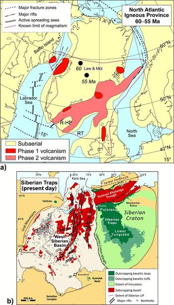
That the Siberian Traps extend over a wider area – approximately twice the size of the North Atlantic Province – is evident from Figure 1, where the two provinces are drawn to the same scale. That these areas are crudely delineated is also indisputable (e.g. it is not known how far the Siberian province extends to the north beneath the Kara Sea, nor how much of the NAIP is located beneath the Greenland icecap), but there is a more fundamental issue that is very difficult to address. This is the continuity of outcrops: were the gaps between far-flung outcrops always there, or were the volcanic rocks removed by erosion? (Similar issues exist for other LIPs, particularly the Central Atlantic magmatic province, which has been associated with the end-Triassic mass extinction.) Despite these uncertainties, several estimates of the volumes of the two provinces exist.
Maps of the North Atlantic and Siberian large igneous provinces, drawn to approximately the same scale, to demonstrate the relative sizes and configurations of the two provinces. (a) North Atlantic Igneous Province at 55–60 Ma, prior to full separation of the North American and Eurasian plates. ‘Law Mul 55 60 Ma’ refer to proposed locations of the axis of the Iceland plume at 55 and 60 Ma (Lawver & Müller, Reference Lawver and Müller1994). Modified after Saunders et al. (Reference Saunders, Fitton, Kerr, Norry, Kent, Mahoney and Coffin1997). (b) Siberian large igneous province (present-day configuration), from Saunders & Reichow (Reference Saunders and Reichow2009). Ur – Urengoy Rift; Kh – Khudosey Rift.

The NAIP has two main phases of volcanism (White & McKenzie, Reference White and McKenzie1989; Saunders et al. Reference Saunders, Fitton, Kerr, Norry, Kent, Mahoney and Coffin1997): an initial phase of pre-break-up continent-based flood basalt volcanism at c. 61 Ma during Chron 26 and, c. 4 million years later, a second, far more voluminous phase of activity associated with the break-up of the NE Atlantic during Chron 24r (beginning at c. 56.5 Ma). The two phases of activity are recorded not only in the lava piles, but also by ash layers in nearby basins such as the North Sea (Knox & Morton, Reference Knox, Morton, Morton and Parson1988). Remnants of the Phase 1 activity are found at very widespread and separate localities (Baffin Island, West Greenland, parts of East Greenland, the lower part of the Faroes lava pile and the Hebridean province; a pre-drift distance of over 2000 km) but, as mentioned above, it is unclear whether the magmatism covered the entire region. Volume estimates are therefore tentative, but are not likely to be less than 50000 km3 (Dickin, Reference Dickin and Macdougall1988) and may well be as much as 150000 km3, depending on whether there are significant volumes of basalt beneath the Greenland ice sheet and on the volume of the oldest flows along the SE Greenland margin. The oldest flows drilled at Site 917, ODP Leg 152 are c. 60 Ma old (Sinton, Hitchen & Duncan, Reference Sinton, Hitchen and Duncan1998). The Phase 1 activity therefore appears to have produced a similar volume of lavas as the Miocene Columbia River Basalt Province (175000 km3; Tolan et al. Reference Tolan, Reidel, Beeson, Anderson, Fecht, Swanson, Reidel and Hooper1989).
Phase 2 activity was, however, much more voluminous. Rifting and separation of Greenland from the Eurasian plate during early Chron 24 time (c. 56 Ma) created two conjugate rifted margins c. 2500 km long, and enabled extensive melting of the mantle. These margins are characterized by voluminous seaward-dipping reflectors (thick sequences of basalts and less-abundant rhyolite) and complementary deep crustal intrusive bodies. It also led to the formation of the bulk of the East Greenland Scoresby Sund basalts (c. 230000 km3; Larsen, Watt & Watt, Reference Larsen, Watt and Watt1989) and the upper part of the Faroes basalt province. The volume of the lavas is difficult to estimate because their thickness is poorly constrained and because it is unclear how much has been lost through erosion. Eldholm & Grue (Reference Eldholm and Grue1994) suggest a figure of 1.8×10⁶ km3 of extrusives (including the Scoresby Sund and Faroes sequences) and a total volume of all igneous material (igneous crust senso lato associated with the continent break-up) of c. 6.6×10⁶ km3, which is within the range of 5–10×106 km3 suggested by White et al. (Reference White, Spence, Fowler, McKenzie, Westbrook and Bowen1987).
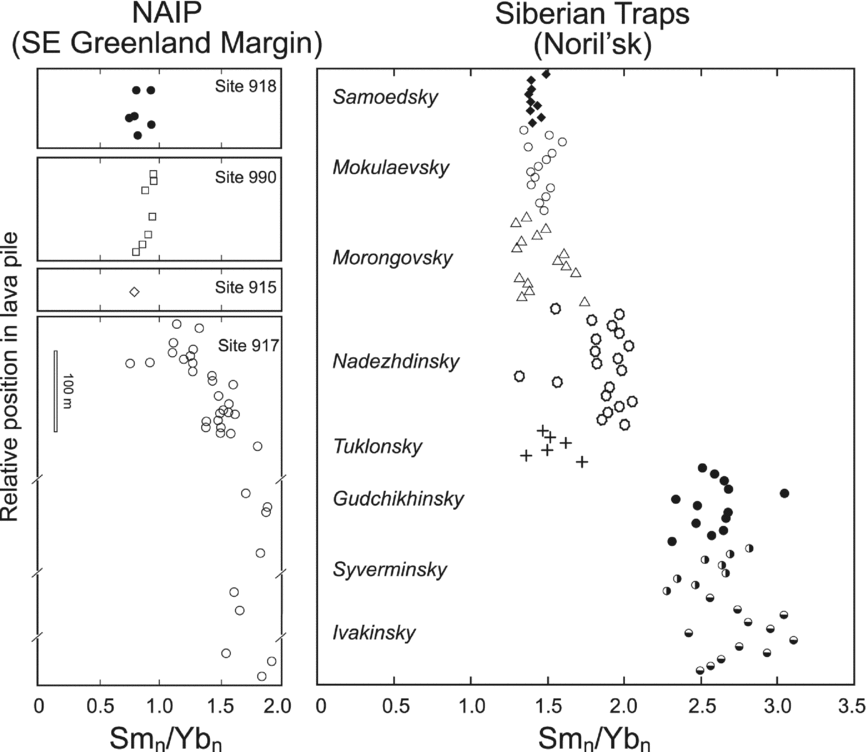
The effects of continent break-up on melt generation can be seen in the composition of the lavas. Figure 2 shows plots of Sm/Yb for composite sections from the SE Greenland margin and Noril'sk in Siberia. This ratio gives an indication of the average depth of melting; Yb is retained by garnet in the mantle source, resulting in a higher Sm/Yb ratio if the average depth of melting is higher (e.g. caused by a thick lithospheric lid). As the lithosphere thinned, by stretching or delamination, the average depth of melting was reduced and the extent of melting increased, reducing the garnet effect and causing Sm/Yb to decrease. This is precisely what is seen in these two geochemical profiles and reported by Fram & Lesher (Reference Fram and Lesher1993, Reference Fram and Lesher1997) and Fram, Lesher & Volpe (Reference Fram, Lesher, Volpe, Saunders, Larsen and Wise1998). As the extent of melting increases, the volume of the melt increases (along with the volume of magmatic volatiles). As a corollary to this, the extent of crustal contamination also shows a marked decrease as the magmatism migrates from continent- to ocean-based (e.g. Saunders et al. Reference Saunders, Fitton, Kerr, Norry, Kent, Mahoney and Coffin1997), and this will have affected the volume and composition of any volatiles released by the activity.
Sm/Yb (chondrite-normalized) in basalts from the NAIP (SE Greenland margin) and Siberian Traps (Noril'sk). The progressive reduction of Sm/Yb upwards through both sequences of basalts suggests temporal shallowing of the average depth of melting, consistent with thinning of the lithosphere due to extension and/or delamination. NAIP plot modified after Saunders, Larsen & Fitton (Reference Saunders, Larsen, Fitton, Saunders, Larsen and Wise1998). Siberian Traps data, including the names of the main lava formations at Noril'sk, from Lightfoot et al. (Reference Lightfoot, Naldrett, Gorbachev, Doherty and Fedorenko1990), Wooden et al. (Reference Wooden, Czamanske, Fedorenko, Arndt, Chauvel, Bouse, King, Knight and Siems1993) and Hawkesworth et al. (Reference Hawkesworth, Lightfoot, Fedorenko, Blake, Naldrett, Doherty and Gorbachev1995).

The likely initiator for the NAIP magmatism was the arrival at the base of the Greenland lithosphere of the proto-Iceland plume at c. 61 Ma (Richards, Duncan & Courtillot, Reference Richards, Duncan and Courtillot1989; Larsen, Yuen & Storey, Reference Larsen, Yuen and Storey1999). This initially caused the relatively small-volume continental flood basalt magmatism and minor uplift (e.g. Saunders et al. Reference Saunders, Jones, Morgan, Pierce, Widdowson and Xu2007). After a short hiatus, plate rupture allowed extensive shallow, decompression melting of the hot plume mantle, voluminous melt generation and greater uplift linked to development of the volcanic rifted margins (Eldholm & Grue, Reference Eldholm and Grue1994; Saunders et al. Reference Saunders, Fitton, Kerr, Norry, Kent, Mahoney and Coffin1997, Reference Saunders, Jones, Morgan, Pierce, Widdowson and Xu2007). Most of the eruptions were subaerial or shallow water along the volcanic rifted margin, hence assisting the release of volatiles into the atmosphere. However, as the margins migrated from the epicentre of the plume (and as the plume's sphere of influence effectively shrank to the vicinity of the Greenland–Faroes Ridge), they became submarine and atmospheric emissions would have been reduced. Along the Greenland–Faroes Ridge the eruptions were likely to have persisted as mostly subaerial, because of the dynamic uplift above the mantle plume. In short, the combination of rifting and rapid decompression of plume mantle created the large melt volumes, which in turn triggered the environmental impact on the late Paleocene climate (Eldholm & Thomas, Reference Eldholm and Thomas1993).
2.a. The PETM
The PETM is a rapid-onset, short-duration, hyperthermal event with pronounced negative oxygen and carbon isotope isotopic excursions (OIE and CIE) (Kennett & Stott, Reference Kennett and Stott1991); a decrease in carbonate productivity associated with shallowing of the carbonate compensation depth and an increase in ocean surface acidification (Zachos et al. Reference Zachos, Röhl, Schellenberg, Sluijs, Hodell, Kelly, Thomas, Nicola, Raffi, Lourens, McCarren and Kroon2005; Penman et al. Reference Penman, Hönisch, Zeebe, Thomas and Zachos2014); a major extinction of benthic foraminfera (Thomas, Reference Thomas and Crame1989; Thomas & Shackleton, Reference Thomas, Shackleton, O'B. Knox, Corfield and Dunay1996); marine anoxia and/or dysoxia (Dickson, Cohen & Coe, Reference Dickson, Cohen and Coe2012; Dickson et al. Reference Dickson, Rees-Owen, Maerz, Coe, Cohen, Pancost, Taylor and Shcherbinina2014); and a major perturbation of global weathering patterns (Ravizza et al. Reference Ravizza, Norris, Blusztajn and Aubry2001; Wieczorek et al. Reference Wieczorek, Fantle, Kump and Ravizza2013). It is one of the most studied of the Cenozoic hyperthermals (e.g. see the review by Cohen, Coe & Kemp, Reference Cohen, Coe and Kemp2007), with over 40 high-resolution deep-sea core sets from ocean drilling, abundant terrestrial sections and good calibration through astronomical cyclicity (Westerhold, Roehl & Laskar, Reference Westerhold, Roehl and Laskar2012). That the Earth's carbon cycle underwent a major perturbation at this time is indicated by the c. 2–4‰ decrease of δ13C preserved in marine carbonates and fossils over a period of a few thousand years or less, and that lasted for c. 170 ka (e.g. Röhl et al. Reference Röhl, Westerhold, Bralower and Zachos2007). This has led to the suggestion that the cause of the PETM and its associated effects was the rapid injection of a large mass of isotopically light carbon (e.g. methane hydrate) into the ocean–atmosphere system (e.g. Dickens et al. Reference Dickens, Oneil, Rea and Owen1995).
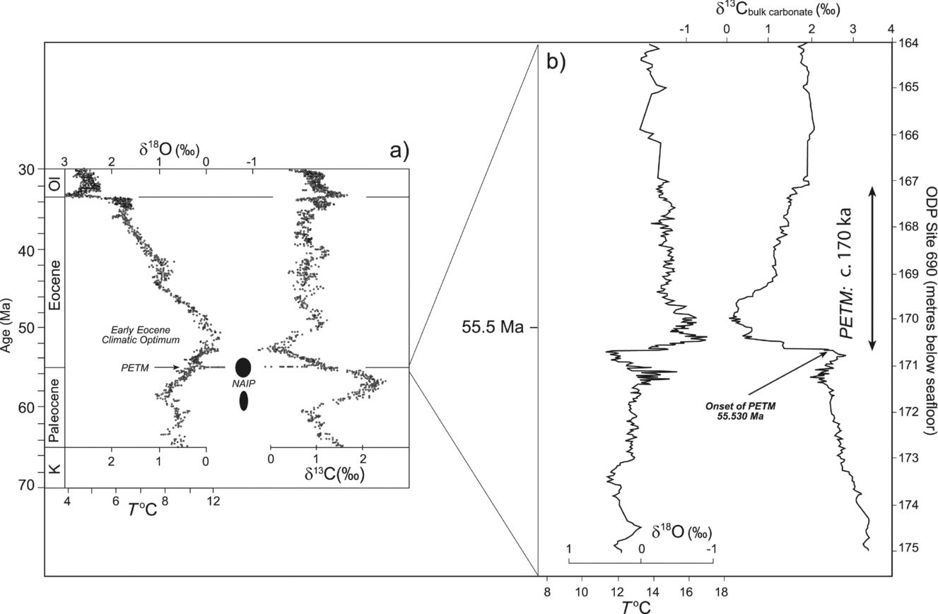
Ocean Drilling Program Site 690 from the Weddell Sea is one of several high-resolution sequences that have provided a detailed section across the PETM, and which illustrates the typical profiles of the carbon and oxygen isotopic excursions (Bains, Corfield & Norris, Reference Bains, Corfield and Norris1999) (Fig. 3). On a broad timescale, the PETM is superimposed on a much longer wavelength variation in carbon and oxygen isotopes (a δ13C change of c. −0.5‰ Ma−1; ΔT of about +0.5°C Ma−1) that is the development of the early Eocene climatic optimum at c. 53 Ma (Fig. 3), and which arguably began at c. 57 Ma. At c. 55.5 Ma (see Section 2.b), δ13C decreased rapidly by c. 2.5‰ at Site 690 over a timescale of less than a few thousand years, although the minimum duration of this decrease is unconstrained. High-resolution core studies suggest that this initial rapid decrease may have occurred over an ‘instantaneous’ period of time (Wright & Schaller, Reference Wright and Schaller2013) and Röhl et al. (Reference Röhl, Westerhold, Bralower and Zachos2007) suggest a timescale of <1 ka. However, from their high-resolution study of an expanded PETM section in central China, Chen et al. (Reference Chen, Wang, Hu, Yang, Zhu, Dong, Tang, Peng and Ding2014) conclude that the interval of rapid decline of δ13C may be considerably longer. δ13C then flatlines for c. 80 ka, before initially recovering rapidly by c. 1‰ and then increasing more slowly to intersect the projected pre-CIE curve. The total duration of the PETM is estimated to be 170 ka, based on astronomical cyclicity (Röhl et al. Reference Röhl, Westerhold, Bralower and Zachos2007) and depending on the positioning of the end of the CIE.
δ13C, δ18O and calculated seawater temperatures during (a) Paleocene–Eocene time and (b) across the PETM. Data in (a) are from Zachos et al. (Reference Zachos, Pagani, Sloan, Thomas and Billups2001) and mostly represent data from specific taxa. Estimates for the age of the NAIP are from Saunders et al. (Reference Saunders, Fitton, Kerr, Norry, Kent, Mahoney and Coffin1997), Storey, Duncan & Swisher (Reference Storey, Duncan and Swisher2007) and Storey, Duncan & Tegner (Reference Storey, Duncan and Swisher2007). Data in panel (b) are from Bains et al. (Reference Bains, Corfield and Norris1999) and are from bulk carbonate analyses. The age of the onset of the PETM is from Westerhold, Roehl & Laskar (Reference Westerhold, Roehl and Laskar2012) and the estimated duration of the PETM is taken from Röhl et al. (Reference Röhl, Westerhold, Bralower and Zachos2007).

In addition to the CIE, the onset of the PETM is marked by a large oxygen isotope excursion that indicates a global surface warming of between 4 and 7°C (Kennett & Stott, Reference Kennett and Stott1991; Bains, Corfield & Norris, Reference Bains, Corfield and Norris1999; Jones et al. Reference Jones, Lunt, Schmidt, Ridgwell, Sluijs, Valdes and Maslin2013). The increase in high-latitude sea-surface temperatures was higher (8–10°C) than their tropical equivalents (4–5°C) (Zachos et al. Reference Zachos, Wara, Bohaty, Delaney, Petrizzo, Brill, Bralower and Premoli-Silva2003). The surface temperature increase migrated to progressively deeper waters, with bottom-water temperatures increasing by as much as 5°C (Zachos et al. Reference Zachos, Wara, Bohaty, Delaney, Petrizzo, Brill, Bralower and Premoli-Silva2003). In addition to the downwards migration of the thermal pulse and CIE (Thomas et al. Reference Thomas, Zachos, Bralower, Thomas and Bohaty2002), there was also a top-down progression of marine acidification (Zachos et al. Reference Zachos, Röhl, Schellenberg, Sluijs, Hodell, Kelly, Thomas, Nicola, Raffi, Lourens, McCarren and Kroon2005), a progressive increase in ocean stratification and a strengthening nutricline (Bralower et al. Reference Bralower, Kelly, Gibbs, Farley, Eccles, Lindemann and Smith2014a , Reference Bralower, Meissner, Alexander and Thomas b ), and suboxic conditions (Pälicke, Delaney & Zachos, Reference Pälicke, Delaney and Zachos2014) leading to the benthic extinction in the warmer deep waters (Thomas, Reference Thomas and Crame1989). Sea levels also rose, consistent with thermal expansion of the ocean (e.g. Handley, Crouch & Pancost, Reference Handley, Crouch and Pancost2011).
The CIE, OIE, ocean acidification and benthic foraminifera extinction appear to coincide in many PETM sections (Katz et al. Reference Katz, Pak, Dickens and Miller1999). However, Sluijs et al. (Reference Sluijs, Brinkhuis, Schouten, Bohaty, John, Zachos, Reichart, Damste, Crouch and Dickens2007) argue that surface-ocean warming, by perhaps as much as 4°C, began before the CIE and acidification events that mark the onset of the PETM. They base their argument on the acme occurrence of the dinoflagellate cyst Apectodinium and the palaeothermometer TEX86 in New Jersey margin sediments that were deposited up to c. 3 ka before the main CIE that marks the onset of the PETM. The acme of Apectodinium also occurs in Pacific and North Sea sections, suggesting that this precursor warming is global in extent. Lacustrine sediments from the Nanyang Basin, central China provide a high-resolution dataset through the CIE, preserved in both organic material and micritic carbonate. Not only does the record indicate that the CIE was developing slowly over several thousands of years prior to the main PETM event, but also that the sediments also show a precursor rise (c. 4°C) in palaeo-air temperatures based on organic molecules from derived soil material (Chen et al. Reference Chen, Wang, Hu, Yang, Zhu, Dong, Tang, Peng and Ding2014). Thomas et al. (Reference Thomas, Zachos, Bralower, Thomas and Bohaty2002) also report evidence for a brief period of warming prior to the CIE of the PETM, although the oxygen isotope data for high-latitude Site 690 suggests a precursor 4°C temperature decrease (Bains, Corfield & Norris, Reference Bains, Corfield and Norris1999).
2.b. Correlation between the PETM and NAIP
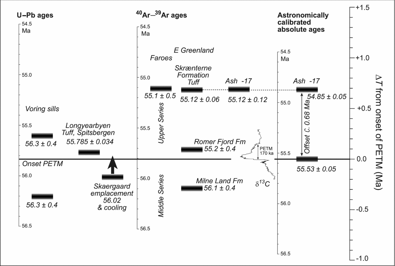
Astronomically calibrated cyclostratigraphy, using new orbital solutions, indicates an absolute age for the onset of the PETM (≡Paleocene–Eocene boundary) of 55.530±0.05 Ma (Westerhold, Roehl & Laskar, Reference Westerhold, Roehl and Laskar2012) (Fig. 4). Can this age be verified by radiometric dating? Some PETM sections contain dateable ash layers, but these tend to overlie the onset of the P–E boundary rather than bracket it, and any radiometric dates (U–Pb or 40Ar–39Ar) on the tuffs have to be extrapolated to the boundary using cyclostratigraphy or estimations of sedimentation rates, with inherent errors. A weighted mean of the five youngest zircons from an ash layer in the Longyearbyen section, Spitsbergen, has yielded a U–Pb age of 55.785±0.034 Ma (Charles et al. Reference Charles, Condon, Harding, Pälike, Marshall, Cui, Kump and Croudace2011). The ash layer is c. 11 m above the base of the PETM, so the age has to be increased by 40–80 ka to determine the age of the onset of the PETM. There is therefore a significant difference of c. 30–250 ka between the younger astronomically tuned age and the extrapolated U–Pb age for the PETM, which Westerhold, Roehl & Laskar (Reference Westerhold, Roehl and Laskar2012) attribute to ageing of the zircons in magma chambers prior to eruption.
Age data associated with the PETM and the Phase 2 activity of the North Atlantic igneous province. Because of discrepancies between 40Ar–39Ar, U–Pb and astronomically calibrated ages, all of the data are referenced relative to the onset of the PETM (right-hand scale). Absolute age scales are adjusted relative to the PETM. The offset between Ash Bed –17 and the PETM is taken from Westerhold, Roehl & Laskar (Reference Westerhold, Roehl and Laskar2012). Data sources: Voring sills: Svensen, Planke & Corfu (Reference Svensen, Planke and Corfu2010); Skaergaard intrusion: Wotzlaw et al. (Reference Wotzlaw, Bindeman, Schaltegger, Brooks and Naslund2012); Longyearbyen Tuff: Charles et al. (Reference Charles, Condon, Harding, Pälike, Marshall, Cui, Kump and Croudace2011); East Greenland and Faroes basalts and Skraenterne Tuff: Storey, Duncan & Swisher (Reference Storey, Duncan and Swisher2007) and Storey, Duncan & Tegner (Reference Storey, Duncan and Swisher2007) (FCs = 28.02 Ma); PETM CIE: Fig. 3; astronomically calibrated ages: Westerhold, Roehl & Laskar (Reference Westerhold, Roehl and Laskar2012).

40Ar–39Ar dating of sanidines has also been used to constrain the age of the P–E boundary. Ash Bed –17 is one of several prominent marker horizons in the North Atlantic region and is again situated above the onset of the PETM. Storey, Duncan & Swisher (Reference Storey, Duncan and Swisher2007) obtained an average sanidine fusion age of 55.12±0.12 Ma for Ash −17 (with a small cluster of possibly xenocrystic ages of c. 56 Ma). The astronomically calibrated age for Ash −17 is, however, significantly younger at 54.850±0.05 Ma and c. 680 ka younger than the astronomically determined value for the PETM (Westerhold, Roehl & Laskar, Reference Westerhold, Roehl and Laskar2012).
Sanidine offers a high-precision dating technique but, because the Ar–Ar method requires calibration using a reference standard (usually Fish Canyon Tuff sanidine, or FCs) and because there is some uncertainty in the potassium decay constant, the errors are inherently greater than the U–Pb method and accuracy is very reliant on the value of FCs that is used. In the study by Storey, Duncan & Swisher (Reference Storey, Duncan and Swisher2007) the data were referenced to FCs 28.02 Ma, but FCs has recently been revised to 28.201 Ma (Kuiper et al. Reference Kuiper, Deino, Hilgen, Krijgsman, Renne and Wijbrans2008). This increases the 40Ar–39Ar age of Ash Bed −17 to 55.473±0.12 Ma, and therefore increases the discrepancy with the astronomical age. Westerhold, Roehl & Laskar (Reference Westerhold, Roehl and Laskar2012) argue that the value for FCs should be reduced to 27.89 Ma, which is within error of the value of 28.02±0.28 Ma determined by Renne et al. (Reference Renne, Swisher, Deino, Karner, Owens and DePaolo1998). Using an FCs of 27.89 decreases the 40Ar–39Ar age of Ash −17 to 54.866±0.12 Ma. This, however, increases the discrepancy between the Ar–Ar and U–Pb dating methods, an issue which grows with distance back in time (e.g. to the P–Tr boundary).
Given that the U–Pb and 40Ar–39Ar ages for the PETM are both older than the astronomical age does beg the question as to whether the astronomical age for the onset of the PETM is too young. Solutions for the astronomical cycles become increasingly complex in older sequences because of the inherent chaos in the orbital solutions, so this is not an unreasonable suggestion.
Notwithstanding these discrepancies in the absolute age of the P–E boundary, the radiometric dates allow us to correlate the P–E boundary with the magmatism of the NAIP (Fig. 4). Ash Bed −17 is petrologically similar to a tuff in the Skrænterne Formation, the uppermost part of the thick pile of Paleocene basalts in east Greenland. The 40Ar–39Ar ages of Ash −17 and the Skrænterne tuff are indistinguishable (both are 55.12 Ma using FCs of 28.02 Ma), and therefore provide an important link between the PETM-bearing sedimentary successions and the NAIP activity in Greenland (Storey, Duncan & Swisher, Reference Storey, Duncan and Swisher2007). Furthermore, 40Ar–39Ar ages on the voluminous, underlying parts of the East Greenland flood basalts bracket the activity between 56.1±0.4 Ma (Milne Land Formation) and 55.2±0.4 Ma (Romer Fjord Fm) (Storey, Duncan & Tegner, Reference Storey, Duncan and Tegner2007), showing that the volcanic activity overlapped with the PETM.
The Skaergaard intrusion in East Greenland intrudes the lower part of the flood basalt lava pile and, it is argued, was crystallizing and cooling while the bulk of the lava pile was emplaced above it, a period that may have been at least as short as 300000 years (Larsen & Tegner, Reference Larsen and Tegner2006). Using zircon U–Pb ages, Wotzlaw et al. (Reference Wotzlaw, Bindeman, Schaltegger, Brooks and Naslund2012) estimate that the intrusion emplacement age is c. 56.02 Ma and that the minimum age for the flood basalt volcanism in East Greenland is 55.960±0.064 Ma, which again coincides with the age of the onset of the PETM given by Charles et al. (Reference Charles, Condon, Harding, Pälike, Marshall, Cui, Kump and Croudace2011). Dolerite sills from the Vøring Basin, Norway, contain zircons with ages of 55.6±0.3 and 56.3±0.4 Ma (Svensen, Planke & Corfu, Reference Svensen, Planke and Corfu2010).
3. The Siberian Traps and the EPME
The Siberian Traps also probably owe their origin to a mantle plume (see reviews by Sharma, Reference Sharma, Mahoney and Coffin1997; Saunders et al. Reference Saunders, England, Reichow and White2005; Sobolev et al. Reference Sobolev, Sobolev, Kuzmin, Krivolutskaya, Petrunin, Arndt, Radko and Vasiliev2011). The bulk of the exposed lavas and pyroclastic deposits are located on the Siberian Craton around Noril'sk, to the east in Meimecha-Kutoy and to the southeast in the Tunguska Basin (Fig. 1). The Meimecha suites are unusual alkali- and magnesium-rich lavas and intrusives, but the majority of the lavas elsewhere are tholeiitic and alkalic basalts (Sharma, Reference Sharma, Mahoney and Coffin1997). Extensive sill complexes are found in the underlying sedimentary basins, and these basins host substantial deposits of evaporate and coal. The sills created a large number of explosion craters that may have been important gas release vents during the EPME (Svensen et al. Reference Svensen, Planke, Polozov, Schmidbauer, Corfu, Podladchikov and Jamtveit2009a ).
Outliers of Siberian Trap activity are found in the northern Urals around Vorkuta, in the Kuzbass, in Taimyr in the Russian arctic and in the southern Urals around Chelyabinsk, although the latter subprovince is probably slightly younger than the main province (Reichow et al. Reference Reichow, Pringle, Al'Mukhamedov, Allen, Andreichev, Buslov, Davies, Fedoseev, Fitton, Inger, Medvedev, Mitchell, Puchkov, Safonova, Scott and Saunders2009). However, the main part of the Siberian province appears to reside beneath the West Siberian Basin, which has major north–south-aligned rifts and has been considered a failed ocean basin. The exact thickness, distribution and volume of the igneous rocks that floor the basin are unknown, but sequences over 1 km thick have been drilled in parts of the basin (Reichow et al. Reference Reichow, Saunders, White, Pringle, Al'Mukhamedov, Medvedev and Korda2002; Saunders et al. Reference Saunders, England, Reichow and White2005).
The total volume of the volcanic sequences associated with the Siberian province is poorly constrained, for the reasons given above. Saunders & Reichow (Reference Saunders and Reichow2009) suggest a ‘working estimate’ of 3×10⁶ km3, plus or minus 1×10⁶ km3. The total volume of the igneous rocks (including lavas, intrusives that ponded within the crust and cumulates associated with magmatic differentiation) would substantially increase these figures. The bulk of the volcanic rocks are evolved, with Mg numbers (Mg/Mg+Fe) less than 0.6 (e.g. Sharma, Reference Sharma, Mahoney and Coffin1997) so, unless the primary melts had unusually low Mg numbers, substantial volumes of cumulate must exist within the crust. As a crude approximation, if we assume that the ratio of extrusive/total volume is the same as the NAIP (i.e. 1.8×10⁶ km3/6.6×106 km3 = 0.27; Eldholm & Grue, Reference Eldholm and Grue1994), then the total volume for the Siberian province would be c. 11×106 km3, assuming an extrusive volume of 3×10⁶ km3 (see Section 4). This is about one-third of the estimated volume of the Ontong Java Plateau (Gladczenko, Coffin & Eldholm, Reference Gladczenko, Coffin and Eldholm1997).
The role of a mantle plume in the formation of the Siberian Province is contentious primarily because, unlike the NAIP and Iceland, there is no obvious modern-day descendent hotspot (although some workers have suggested that the Iceland hotspot could fill this role; Smirnov & Tarduno, Reference Smirnov and Tarduno2010). Furthermore, the Siberian Province does not show clear evidence of surface uplift (Czamanske et al. Reference Czamanske, Gurevitch, Fedorenko and Simonov1998) that would be expected from the emplacement of a hot start-up plume (Campbell & Griffiths, Reference Campbell and Griffiths1990). However, Sobolev et al. (Reference Sobolev, Sobolev, Kuzmin, Krivolutskaya, Petrunin, Arndt, Radko and Vasiliev2011) have proposed that the plume may have contained a significant proportion of dense eclogite that reduced the dynamic uplift (see also Cordery, Davies & Campbell, Reference Cordery, Davies and Campbell1997) and that the plume also stripped the base of the lithosphere, effectively making space for it to ascend and decompress (a form of delamination, also espoused by Elkins-Tanton, Reference Elkins-Tanton2007).
As for the basalt sequences in the NAIP, the Siberian Traps also show evidence of broad shallowing and decompression of the melt zone in the mantle in response to either rifting and extension (Saunders et al. Reference Saunders, England, Reichow and White2005), delamination (Elkins-Tanton, Reference Elkins-Tanton2007) or lithosphere erosion (Sobolev et al. Reference Sobolev, Sobolev, Kuzmin, Krivolutskaya, Petrunin, Arndt, Radko and Vasiliev2011). Figure 2 includes variation of Sm/Yb through the Noril'sk succession. Several of the formations are strongly contaminated by continental crust, but the Sm/Yb relationships are preserved. Overall, the Sm/Yb values in Noril'sk are higher than those for the NAIP sequence, which is consistent with the thicker lithosphere beneath the Noril'sk region and the lack of development of an ocean basin in that area. However, the data in Figure 2 indicate that the basalts melts were probably not generated below the thick Siberian Craton, a region of Archaean lithosphere with a present-day thermal thickness in excess of 300 km (Artemieva & Mooney, Reference Artemieva and Mooney2001). Rather, they were likely to have formed in the rifted basins to the west of the craton and flowed eastwards onto the craton. This would entail uplift, possibly plume-assisted, of the lithosphere beneath the West Siberian Basin (e.g. Saunders et al. Reference Saunders, England, Reichow and White2005). Any record of this syn-volcanic uplift is, unfortunately, now buried beneath the thick sedimentary fill.
3.a. The EPME
The mass extinction that occurred near the end of the Permian was the most severe that the Earth has known, destroying as much as 96% of marine species (Raup, Reference Raup1979; Benton, Reference Benton2003; Erwin, Reference Erwin2005). It particularly affected benthic fauna, possibly through immersion in dysoxic, anoxic or even euxinic seawater, but over two-thirds of land-based reptile and amphibian families and a substantial fraction of insects and land plants were also lost (Wignall & Twitchett, Reference Wignall and Twitchett1996).
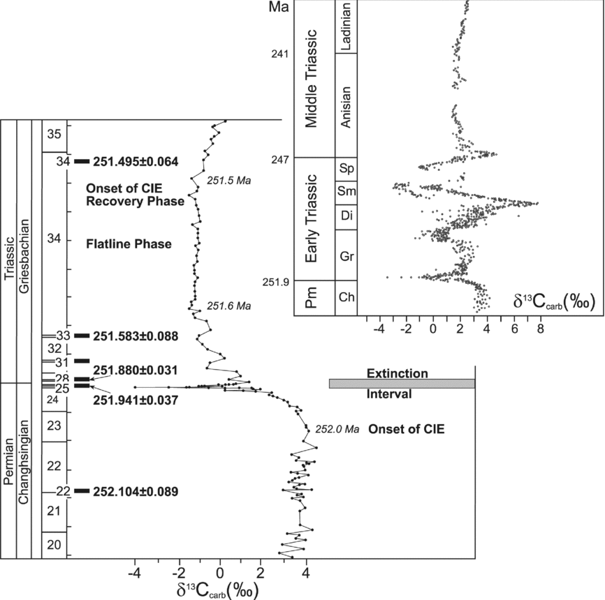
Permo-Triassic boundary sections in southern China, including the GSSP at Meishan, contain numerous zircon- and sanidine-bearing volcanic ash layers derived from local contemporaneous silicic, explosive eruptions. These ash layers are located both above and below the main event horizons, enabling precise bracketing of the events (Fig. 5). Five of these ash layers have yielded a high-precision U–Pb timeline for the culmination of the mass extinction event recorded in the P–Tr global boundary stratotype section and point at Meishan. These have recently enabled Shen et al. (Reference Shen, Crowley, Wang, Bowring, Erwin, Sadler, Cao, Rothman, Henderson, Ramezani, Zhang, Shen, Wang, Wang, Mu, Li, Tang, Liu, Liu, Zeng, Jiang and Jin2011), Burgess, Bowring & Shen (Reference Burgess, Bowring and Shen2014) and Wang et al. (Reference Wang, Sadler, Shen, Erwin, Zhang, Wang, Wang, Crowley and Henderson2014) to place important constraints on the onset and duration of the CIE and the mass extinction. The main extinction event recorded at Meishan began just below Bed 25 (251.941±0.037 Ma) and was complete by Bed 28 (251.880±0.031 Ma), an interval estimated to be 61±48 ka (Burgess, Bowring & Shen, Reference Burgess, Bowring and Shen2014). This is considered to be a maximum duration, because the Meishan section at this level is condensed.
High-precision U–Pb ages for zircons from ash horizons at the Meishan GSSP, China (Burgess, Bowring & Shen Reference Burgess, Bowring and Shen2014). Carbon isotope data from Cao, Wang & Jin (2002) and Cao et al. (Reference Cao, Love, Hays, Wang, Shen and Summons2009); extinction interval from Shen et al. (Reference Shen, Crowley, Wang, Bowring, Erwin, Sadler, Cao, Rothman, Henderson, Ramezani, Zhang, Shen, Wang, Wang, Mu, Li, Tang, Liu, Liu, Zeng, Jiang and Jin2011) and Wang et al. (Reference Wang, Sadler, Shen, Erwin, Zhang, Wang, Wang, Crowley and Henderson2014). Inset: Composite δ13C isotope curve for late Permian – Middle Triassic time, demonstrating strong fluctuations in the global carbon isotope record throughout Early Triassic time (modified from Payne et al. Reference Payne, Lehrmann, Follett, Seibel, Kump, Riccardi, Altiner, Sano and Wei2007). Pm – Permian; Ch – Changhsingian; Gr – Griesbachian; Di – Dienerian; Sm – Smithian; Sp – Spathian.

Wang et al. (Reference Wang, Sadler, Shen, Erwin, Zhang, Wang, Wang, Crowley and Henderson2014) compiled data on 1450 species from 18 sections from south China and northern Gondwana, and integrated these with the radiometric data of Shen et al. (Reference Shen, Crowley, Wang, Bowring, Erwin, Sadler, Cao, Rothman, Henderson, Ramezani, Zhang, Shen, Wang, Wang, Mu, Li, Tang, Liu, Liu, Zeng, Jiang and Jin2011). They observe an abrupt extinction of 62% of species over the 61±48 ka interval between Beds 25 and 28. However, Song et al. (Reference Song, Wignall, Tong and Yin2013b ) report two pulses of extinction, the first in the latest Permian deposits at Bed 25 and the second in the Lower Triassic deposits at Bed 28. This suggests that rather than a prolonged period of crisis there were at least two extinction pulses, perhaps with fundamentally different environmental causes, with brief periods of recovery in between.
Wang et al. (Reference Wang, Sadler, Shen, Erwin, Zhang, Wang, Wang, Crowley and Henderson2014) also suggest that environmental conditions were deteriorating from c. 1.2 Ma before the sudden extinction. The authors point out that this requires further testing but it is also suggested by Cao et al. (Reference Cao, Love, Hays, Wang, Shen and Summons2009), who observe evidence of major changes in planktic ecology, specifically the radiolarians, well before the main extinction horizon.
There is a substantial volume of literature dealing with the carbon isotope excursions at the end of Permian time and during Early Triassic time. For example, Korte & Kozur (Reference Korte and Kozur2010) list over 120 Permo-Triassic sections and cores where the carbon isotope profile has been described, many by more than one study (c. 20 for the Meishan GSSP alone). While most are marine, the list also includes 28 non-marine sections. There are significant variations in the magnitude and even the stratigraphic position of the anomalies, but a broad consensus has emerged about the general shape of the CIE (Fig. 5) (Retallack & Krull, Reference Retallack, Krull, Greb and DiMichele2006; Korte & Kozur, Reference Korte and Kozur2010).
Before the onset of the CIE, Permian Palaeotethyan marine carbonate typically gives values of δ13C of between +3.5 and +4‰. The rapid decline to −4‰ (Cao et al. Reference Cao, Love, Hays, Wang, Shen and Summons2009) and subsequent recovery has a duration of 2.1–18.8 ka, fluctuates by 1–2‰ for the succeeding c. 0.5 Ma and then flatlines for 63±89 ka (Burgess, Bowring & Shen, Reference Burgess, Bowring and Shen2014). On a longer timescale, δ13Ccarbonate oscillates dramatically by more than 11‰ throughout Early Triassic time, before stabilizing at 2‰ in the early part of Middle Triassic time (Payne et al. Reference Payne, Lehrmann, Wei, Orchard, Schrag and Knoll2004; Payne & Kump, Reference Payne and Kump2007) (Fig. 5). The magnitude of the negative CIE preserved in Beds 24 and 25 at Meishan is of the order of 7–8‰. This compares with average values for the end-Permian CIE in marine and non-marine carbonate of −4.1±1.6‰ (n = 22) and −10.4±2.4‰ (n=3), respectively; the average δ13C excursion in marine organic material is −6.5±3.6‰ (n=14) (Retallack & Krull, Reference Retallack, Krull, Greb and DiMichele2006).
At Meishan, the CIE begins in Bed 23, before the main mass extinction horizon (Fig. 5). In other areas, however, the opposite is true. For example, in their study of the P–Tr boundary section in Jameson Land, East Greenland, Twitchett et al. (Reference Twitchett, Looy, Morante, Visscher and Wignall2001) demonstrate that the CIE occurs after the major collapse of the terrestrial and marine ecosystems. Whatever caused the CIE at this locality cannot therefore have been responsible for the mass extinction event there. The CIE in the expanded carbonate sequence recovered in the Gartnerkofel-1 core began, like the CIE in Meishan, during late Permian time, but the main excursion occurs above the designated P–Tr boundary and, by implication, after the mass extinction horizon (Holser et al. Reference Holser, Schönlaub, Attrep, Boeckelmann, Klein, Magaritiz, Orth, Fenninger, Jenny, Kralik, Mauritsch, Pak, Schramm, Stattegger and Schmöller1989). Wignall & Newton (Reference Wignall and Newton2003) also argue that the mass extinction began before the CIE in sections from Tibet and British Columbia. Interestingly, the mass extinction appears to occur at different time in these areas; the section in British Columbia, which was located on a deep-water margin to Panthalassa, occurred c. 0.5 Ma before the extinction in Tibet, located at high palaeolatitude in the partially enclosed Neotethys. Indeed, the Tibetan section shows a marked increase in diversity associated with ocean warming before the delayed extinction during Early Triassic time.
Marine anoxia was a prevailing and arguably defining condition around the time of the EPME. The anoxia extended to both high and low palaeolatitudes (Wignall & Twitchett, Reference Wignall and Twitchett1996) over a range of water depths from the deep Panthalassia Ocean (Isozaki, Reference Isozaki1997; Takahashi et al. Reference Takahashi, Oba, Kaiho, Yamakita and Sakata2009; Algeo et al. Reference Algeo, Chen, Fraiser and Twitchett2011a , Reference Algeo, Kuwahara, Sano, Bates, Lyons, Elswick, Hinnov, Ellwood, Moser and Maynard b ; Shen et al. Reference Shen, Algeo, Zhou, Feng, Yu and Ellwood2012; Takahashi et al. Reference Takahashi, Yamasaki, Ogawa, Kimura, Kaiho, Yoshida and Tsuchiya2014) to above the storm wave base on the continental shelves (Wignall & Twitchett, Reference Wignall and Twitchett1996). At times, and especially during the main extinction event, the anoxia developed into euxinia which shoaled into the photic zone (Grice et al. Reference Grice, Cao, Love, Bottcher, Twitchett, Grosjean, Summons, Turgeon, Dunning and Jin2005; Riccardi, Arthur & Kump, Reference Riccardi, Arthur and Kump2006; Riccardi et al. Reference Riccardi, Kump, Arthur and D'Hondt2007) and may even have broached the ocean surface, releasing H2S into the atmosphere (Kump, Pavlov & Arthur, Reference Kump, Pavlov and Arthur2005). It is unclear whether photic zone euxinia was restricted to the Palaeotethys (Takahashi et al. Reference Takahashi, Kaiho, Oba and Kakegawa2010) or was global in occurrence, although euxinic conditions do appear to have occurred in the deeper parts of Panthalassa (e.g. Takahashi et al. Reference Takahashi, Yamasaki, Ogawa, Kimura, Kaiho, Yoshida and Tsuchiya2014).
The relative timings of the onset the oceanic anoxia, the carbon isotope excursions and the mass extinction event are not consistent across the globe. In sections from the Panthalassic Ocean, for example, euxinia, anoxia or dysoxia began during late Permian time, well before the CIE and mass extinction horizons (Takahashi et al. Reference Takahashi, Yamasaki, Ogawa, Kimura, Kaiho, Yoshida and Tsuchiya2014). In some sections from the margins of Tethys however, onset of dysoxia is coincident with local benthic extinctions (e.g. Wignall & Hallam, Reference Wignall and Hallam1992; Wignall, Morante & Newton, Reference Wignall, Morante and Newton1998) and there is the major diachroneity documented by Wignall & Newton (Reference Wignall and Newton2003). These findings are broadly consistent with anoxia (senso lato) being a persistent and long-lived feature in the major ocean basins, but having a more intermittent effect on the shallower margins or in more enclosed peri-continental basins. In such a system, globally diachronous onset of anoxia – and extinction – may be expected.
The Permo-Triassic superanoxic event has been described as a protracted Strangelove Ocean (Rampino & Caldeira Reference Rampino and Caldeira2005), where the biological pump between benthic and surface systems completely failed. This, however, is questioned by data published by Meyer et al. (Reference Meyer, Yu, Jost, Kelley and Payne2011), Payne & Clapham (Reference Payne and Clapham2012) and Song et al. (Reference Song, Tong, Algeo, Horacek, Qiu, Song, Tian and Chen2013a ), where vertical depth gradients in δ13C are recorded in some Lower Triassic sequences.
Brennecka et al. (Reference Brennecka, Herrmann, Algeo and Anbar2011) use variations in 235U/238U and Th/U ratios in marine carbonates to measure ocean redox conditions to demonstrate that the oceanic anoxia coincided with, or only slightly preceded, the main extinction horizon. The advantage of this technique is that it provides a record of global ocean conditions rather than a more parochial snapshot. These findings challenge previous suggestions of an extended period of widespread anoxia prior to the end-Permian extinction (e.g. Isozaki, Reference Isozaki1997; Cao et al. Reference Cao, Love, Hays, Wang, Shen and Summons2009).
The evidence for a rise in seawater temperature at the time of the EPME was, until recently, less clear than for the PETM (see review by Twitchett, Reference Twitchett, Williams, Haywodd, Gregory and Schmidt2007). The global temperature rise from measurements of δ18O in marine carbonates (Holser et al. Reference Holser, Schönlaub, Attrep, Boeckelmann, Klein, Magaritiz, Orth, Fenninger, Jenny, Kralik, Mauritsch, Pak, Schramm, Stattegger and Schmöller1989) is of the order of 5–6°C, although the data should be treated with caution as marine carbonates are susceptible to diagenetic alteration. However, the temperature rise accords with the climate model of Kidder & Worsley (Reference Kidder and Worsley2004) and with estimates of tropical sea-surface temperatures based on climatic proxies (e.g. Cui & Kump Reference Cui and Kump2014). Recently however, Sun et al. (Reference Sun, Joachimski, Wignall, Yan, Chen, Jiang, Wang and Lai2012) and Chen et al. (Reference Chen, Joachimski, Shen, Lambert, Lai, Wang, Chen and Yuan2013) used oxygen isotopes from conodont apatite (arguably more resistant to the effects of diagenesis and recrystallization than carbonates) to indicate that there was a decrease of δ18O by as much as 4‰ across P–Tr boundary sections in central and southern China. These were equated to a seawater temperature rise of c. 15°C, assuming that the Earth had no major ice caps at that time. The global thermal system continued to oscillate powerfully until the end of Spathian time, but temperatures remained at potentially lethal levels (at least at low latitudes) throughout much of Early Triassic time. Such increases in temperature would account for the contemporaneous sea-level rise which, through thermal expansion of seawater alone, would be of the order of 20 m (Kidder & Worsley, Reference Kidder and Worsley2004).
As with the PETM, there is evidence for ocean acidification around the time of the P–Tr boundary recorded, for example, in carbonate dissolution on the surfaces on shallow-water skeletal carbonates (Payne et al. Reference Payne, Lehrmann, Follett, Seibel, Kump, Riccardi, Altiner, Sano and Wei2007). Evidence is less clear-cut, however, than for the PETM (Hönisch et al. Reference Hönisch, Ridgwell, Schmidt, Thomas, Gibbs, Sluijs, Zeebe, Kump, Martindale, Greene, Kiessling, Ries, Zachos, Royer, Barker, Marchitto, Moyer, Pelejero, Ziveri, Foster and Williams2012). Fraiser & Bottjer (Reference Fraiser and Bottjer2007) and Payne et al. (Reference Payne, Turchyn, Paytan, DePaolo, Lehrmann, Yu and Wei2010) argue that the acidification was driven by an atmospheric increase in CO2, similar to the events at the PETM, as opposed to (for example) the development of a strongly stratified (Strangelove) ocean with a calcium-carbonate-undersaturated lower layer.
3.b. Correlation between the Siberian Traps and the EPME
There is a lack of high-precision U–Pb dates from the Siberian Traps and associated intrusives. A sill from the Nepa region gives a U–Pb zircon age of 252.0±0.4 Ma (Svensen et al. Reference Svensen, Planke, Polozov, Schmidbauer, Corfu, Podladchikov and Jamtveit2009a ) and a gabbro from Noril'sk an age of 251.2±0.3 Ma (Kamo, Czamanske & Krogh, Reference Kamo, Czamanske and Krogh1996). Basalts from Meimecha-Kotuy have ages ranging from 250.2 to 251.7 Ma (Kamo et al. Reference Kamo, Czamanske, Amelin, Fedorenko, Davis and Trofimov2003), but the relationship between the magmatism at Meimecha and the flood basalts around Noril'sk, Tunguska and the West Siberian Basin is poorly constrained. At the 2013 AGU Fall Meeting, Burgess and Bowring (unpub. data) reported high-precision U-Pb dates from Meimecha and Noril'sk that ‘. . .suggest that intrusive and extrusive magmatism began within analytical uncertainty of the onset of mass extinction, permitting a causal connection with age precision at the ~ ± 0.06 Ma level.’ The publication and interpretation of these new ages is eagerly awaited.
High-precision 40Ar–39Ar dating of sanidines extracted from the ash layers at the Meishan GSSP give significantly younger ages than the co-existing zircons, a problem only partly alleviated by using the revised value for FCs of 28.20 Ma (and made substantially worse if the FCs value of 27.89 Ma as suggested by Westerhold, Roehl & Laskar Reference Westerhold, Roehl and Laskar2012 is used). Beds 25 and 28 that bracket the CIE and the mass extinction horizon give 40Ar–39Ar ages (corrected to FCs of 28.201 Ma) of 251.43±0.15 Ma and 250.85±0.14 Ma, respectively (Renne & Basu, Reference Renne and Basu1991; Renne et al. Reference Renne, Zichao, Richards, Black and Basu1995; Reichow et al. Reference Reichow, Pringle, Al'Mukhamedov, Allen, Andreichev, Buslov, Davies, Fedoseev, Fitton, Inger, Medvedev, Mitchell, Puchkov, Safonova, Scott and Saunders2009). These compare with U–Pb ages of 251.941±0.037 Ma and 251.88±0.031 Ma for Beds 25 and 28 (Burgess, Bowring & Shen, Reference Burgess, Bowring and Shen2014). Not only are the 40Ar–39Ar ages younger, but the difference in ages between Beds 25 and 28 (580±210 ka) is significantly greater than that determined by U–Pb dating (61±48 ka). Hopefully this inconsistency will be explained by further work in progress.
Basalts from Noril'sk, Tunguska, Kuznetz Basin, Vorkuta in the northern Urals, Taimyr and the West Siberian Basin have 40Ar–39Ar ages for plagioclase separates that overlap with the ages of sanidines from ash Beds 25 and 28 at Meishan (e.g. Renne et al. Reference Renne, Zichao, Richards, Black and Basu1995; Reichow et al. Reference Reichow, Saunders, White, Pringle, Al'Mukhamedov, Medvedev and Korda2002, Reference Reichow, Pringle, Al'Mukhamedov, Allen, Andreichev, Buslov, Davies, Fedoseev, Fitton, Inger, Medvedev, Mitchell, Puchkov, Safonova, Scott and Saunders2009). The errors on these 40Ar–39Ar plagioclase dates are greater than for sanidines, meaning that it is not possible to resolve the range of magmatic activity to much better than a million years or so using this dating technique. A detailed review of the dating of the Siberian Traps is given by Ivanov et al. (Reference Ivanov, He, Yan, Ryabov, Shevko, Palesskii and Nikolaeva2013) who conclude that the magmatism may have persisted well into Triassic time.
4. Discussion
In his book, Hallam (Reference Hallam2005) mentions that Alan Charig of the Natural History Museum alluded to the fact over 90 ‘kill mechanisms’ have been proposed as causes of the extinction of the dinosaurs. Similarly, a large number of mechanisms have been suggested for the EPME and the PETM. A review of all these is fortunately beyond the remit of this paper. Even if we restrict the discussion to the contributions from volcanism, there is still a bewildering array of kill mechanisms that can be marshalled.
-
1. Primary mechanisms are where volcanism and its associated products directly impact on the surface environment. These include release of volcanic CO2 (leading to global warming and ocean acidification) and SO2 and ash (global cooling) and halogens (Cl, F; potential degradation of the ozone layer). Also included here is the production and release of thermogenic carbon (CH4, CO2, CO), halogens and organo-halogens by injection of sills into carbonates, evaporate or organic-rich sediments, again leading to global warming and possibly ozone depletion.
-
2. Secondary mechanisms are caused by the primary mechanisms. Thus, warming of oceans (by increasing atmospheric CO2 levels) may trigger breakdown of seafloor and permafrost clathrates and release of CO2 and CH4. Reduction of the ozone layer may lead to increased penetration of ultraviolet light, leading to enhanced mutation rates. Warming of oceans may lead to sluggish thermohaline circulation and development of ocean anoxia. Increased weathering may lead to an enhanced supply of nutrients to the ocean, leading to eutrophication and hypoxia (e.g. Grard et al. Reference Grard, Francois, Dessert and Goddéris2005).
4.a. Gas fluxes
Magmas transport large masses of dissolved gases from the mantle to the surface. In the case of flood basalts, these include H2O, various carbon and sulphur species and halogens. The content of the gas in the magma is a function of the composition and conditions of melting of the source and the nature of any contamination as the magmas travel to the surface. Because magmas may have partly or completely degassed before they vent onto the surface, estimates of the original magmatic volatile content are reliant on direct petrological measurements of undegassed melt inclusions trapped inside phenocrysts (Thordarson et al. Reference Thordarson, Self, Oskarsson and Hulseboch1996; Thordarson & Self, Reference Thordarson and Self2003; Self, Thordarson & Widdowson, Reference Self, Thordarson and Widdowson2005; Self et al. Reference Self, Widdowson, Thordarson and Jay2006, Reference Sharma, Mahoney and Coffin2008; Blake et al. Reference Blake, Self, Sharma and Sephton2010; Black et al. Reference Black, Elkins-Tanton, Rowe and Peate2012), extrapolation of measurements of gas fluxes at modern vents or proxy methods using relationships between melt composition and predicted un-degassed gas content (calibrated by measurement of un-degassed melt inclusions; Blake et al. Reference Blake, Self, Sharma and Sephton2010).
Given the number of parameters that can affect volatile content, and the limitations of methods to measure them, it is unsurprising that estimates of gas masses released from flood basalt eruptions vary widely. Furthermore, the limitations on the precise duration pattern of magmatism severely restrict our understanding of the emission rates, a key requirement for determining the impact of volatiles on the ESCC.
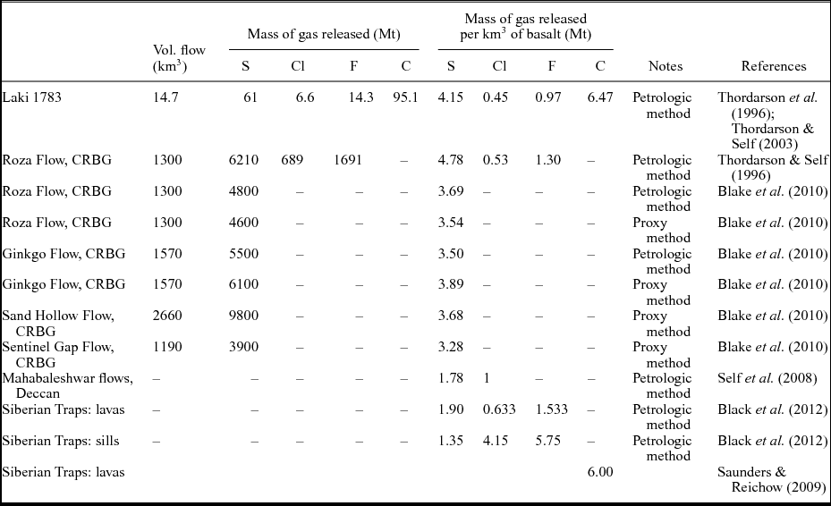
Estimates of the masses of S, Cl, F and C released from the 1783 Laki eruption (Iceland) and flows from the Columbia River Basalt Group, Deccan Traps and Siberian Traps are given in Table 1. These estimates take into account the volatile content of the magma from direct analysis of melt inclusions (or, in the case of some S data, from proxy calculations) and the proportion of gas that is degassed on eruption. Despite the wide range of values, it is evident that on the basis of even the most conservative calculations, the mass of S, Cl and F released from a province such as the Siberian Traps, NAIP (Table 2) and Deccan is prodigious (Thordarson & Self, Reference Thordarson and Self1996; Self et al. Reference Self, Widdowson, Thordarson and Jay2006, Reference Sharma, Mahoney and Coffin2008; Blake et al. Reference Blake, Self, Sharma and Sephton2010; Black et al. Reference Black, Elkins-Tanton, Rowe and Peate2012). These values may be considerably greater if, for example, thermogenic S, Cl and F is released from the contact aureoles of sills emplaced into evaporate- and carbonate-rich sedimentary rocks (Ganino & Arndt, Reference Ganino and Arndt2009; Svensen et al. Reference Svensen, Planke, Polozov, Schmidbauer, Corfu, Podladchikov and Jamtveit2009a ,Reference Svensen, Schmidbauer, Roscher, Stordal and Planke b ).
Estimates of masses of volatile elements released from flood basalts. The petrologic method involves direct analysis of glass melt inclusions and matrix glass; the proxy method employed by Blake et al. (Reference Blake, Self, Sharma and Sephton2010) allows estimate of gas content by using whole-rock iron content to estimate the amount of sulphur in the magma where suitable melt inclusions may not be present.

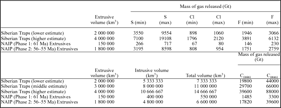
Estimated total masses of gas released from the North Atlantic and Siberian LIP magmas. C(min) assumes 70% degassing, 0.5 wt% C in original magma; C(max) assumes 90% degassing, 0.9 wt% C in original magma. Figures do not include any gas production from thermogenic or secondary processes.

Data for C output are scarce, because the gas (as CO2 or CO) is released from the melt during the early stages of ascent and decompression and is therefore difficult to determine in erupted units. Saunders & Reichow (Reference Saunders and Reichow2009) estimate that a 1000 km3 flow of basalt could release 6 GtC, assuming a magmatic C content of 9000 ppm and a release efficiency of 90%. This compares with c. 5 MtC km−3 for Hawaiian basalt (McCartney, Huffman & Tredoux, Reference McCartney, Huffman, Tredoux, Sharpton and Ward1990) and 5.6–6.5 MtC km−3 released from the 1783 Laki magma (Thordarson et al. Reference Thordarson, Self, Oskarsson and Hulseboch1996; Hartley et al. Reference Hartley, Maclennan, Edmonds and Thordarson2014). Again, these outputs may be substantially increased by injection of sills and dykes into organic-rich (e.g. coal, methane hydrate) or carbonate-rich country rocks, releasing C as CO2, CO or CH4 (Svensen et al. Reference Svensen, Planke, Malthe-Sørenssen, Jamtveit, Myklebust, Eidem and Rey2004, Reference Svensen, Planke, Polozov, Schmidbauer, Corfu, Podladchikov and Jamtveit2009a ,Reference Svensen, Schmidbauer, Roscher, Stordal and Planke b ; Retallack & Jahren, Reference Retallack and Jahren2008; Aarnes et al. Reference Aarnes, Svensen, Connolly and Podladchikov2010; Ogden & Sleep, Reference Ogden and Sleep2012).
Cryptic degassing may also play a role. The larger proportion of a LIP is intrusive rather than extrusive and, if gas can escape from these bodies, it will substantially add to the budget of volatiles. Armstrong McKay et al. (Reference Armstrong McKay, Tyrrell, Wilson and Foster2014) estimate that the total C output from the subaerial lavas of the Columbia River Basalts ranges from 230 to 970 Gt, depending on the proportion of degassing and the amount of crustal contamination of the magmas. If the intrusive rocks are included, this increases to between 1470 and 6190 GtC. There are large uncertainties in these estimates, because (1) the volume of the intrusives and (2) the fraction of CO2 released from the deeper parts of the system are both poorly constrained. For example, in the case of the Columbia River Basalt Group, the volume of intrusives may range between 420000 and 1335000 km3, depending on whether the estimates are based on petrological modelling or seismic refraction profiling (Armstrong McKay et al. Reference Armstrong McKay, Tyrrell, Wilson and Foster2014). A further uncertainty is caused by the possibility of ‘double accounting’; in other words, at least some cumulates in the crust may have yielded their carbon to the associated fractionated melts.
For the purpose of this exercise I assume that the original magma contained between 5000 and 9000 ppm C and that degassing efficiency ranged between 70 and 90% (Table 2). The ratio used for extrusives to total igneous volume is 3.7 (the estimate for the volcanic rifted margins in the North Atlantic; Eldholm & Grue, Reference Eldholm and Grue1994). This value is probably conservative. The range of estimated C outputs from the Siberian Traps is from 20000 Gt (low magma volume) to 88000 Gt (high volume) and for the NAIP (Phase 2) from 18000 to 40000 Gt (Table 2). Note that these figures do not include any additional contribution from thermogenic processes. It is interesting to note that Sobolev et al. (Reference Sobolev, Sobolev, Kuzmin, Krivolutskaya, Petrunin, Arndt, Radko and Vasiliev2011) also suggest that high-CO2 mantle plume source components may have released 46000 GtC during Siberian Trap events, so the estimates in Table 2 may not be excessive. The data do however show that, although there is considerable uncertainty in the masses of volatiles released, the potential upper limits are highly significant in terms of the masses required to cause changes to the ESCC.
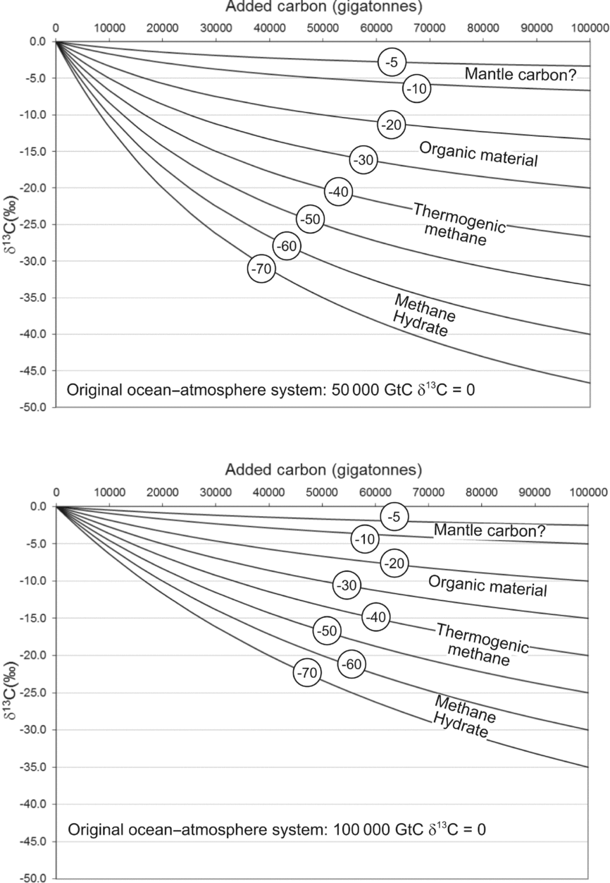
It may be argued that volcanic gas alone cannot produce the CIEs seen at the PETM and EPME. The measured δ13C of volcanic gas and, by implication, the upper mantle is generally no lighter than −10‰ and typically −5‰. This means that to reduce the δ13C of the atmosphere–ocean system by, say, 1‰ requires a mass of 12 times as much volcanic carbon with a value of −5‰ than methane hydrate with a value of −60‰ (Fig. 6). However, this assumes that the δ13C of flood basalts is c. −5‰. Assumptions about basaltic δ13C are based on measurements of mid-ocean ridge basalt, upper mantle material, back-arc basins and Hawaii (Des Marais & Moore, Reference Des Marais and Moore1984; Mattey et al. Reference Mattey, Carr, Wright and Pillinger1984), but to my knowledge no information on the δ13C value of flood basalts exists. Coltice, Simon & Lecuyer (Reference Coltice, Simon and Lecuyer2004) note that a ‘hidden’ reservoir of light carbon likely resides in the deep Earth and, given that the mantle conditions that give rise to flood basalts are unusual, possibly involving deeply sourced start-up plumes, it is perhaps not unreasonable to suggest that their carbon isotope signature may also be unusual and lower than estimated. Deines (Reference Deines2002) notes that a significant fraction of the carbon in many mantle xenoliths has δ13C values as low as −25‰ (see also Hansen, Reference Hansen2006; Dal Corso et al. Reference Dal Corso, Mietto, Newton, Pancost, Preto, Roghi and Wignall2012), and Sobolev et al. (Reference Sobolev, Sobolev, Kuzmin, Krivolutskaya, Petrunin, Arndt, Radko and Vasiliev2011) have suggested that the Siberian Traps were sourced from plume that contained carbon as light as −12‰.
Carbon–carbon isotope mixing lines for sources with different δ13C isotope values added to ocean–atmosphere systems containing: (a) 50000 GtC (δ13C = 0); and (b) 100000 GtC (δ13C = 0). Each mixing curve has a designated δ13C value; the δ13C fields for the main carbon sources are from Maslin & Thomas (Reference Maslin and Thomas2003). For example, in (a) the addition of 10000 Gt (x axis) of carbon from methane hydrate (δ13C −60‰) will decrease the δ13C of this ocean–atmosphere system by 10‰ (y axis).

There is now a well-rehearsed argument that release of large masses (>4000 GtC) of methane hydrate from permafrost and the ocean floor is able to explain the carbon isotope excursions at the PETM and EPME (Dickens et al. Reference Dickens, Oneil, Rea and Owen1995; Benton & Twitchett, Reference Benton and Twitchett2003; Racki & Wignall, Reference Racki and Wignall2005; Retallack & Krull, Reference Retallack, Krull, Greb and DiMichele2006; Dunkley Jones et al. Reference Dunkley Jones, Ridgwell, Lunt, Maslin, Schmidt and Valdes2010). Methane hydrates have low δ13C (c. –60‰) (Kvenvolden, Reference Kvenvolden2002) and they can, in theory, release a large amount of carbon (as methane) rapidly; there is a strong positive feedback. This has been used to explain the magnitude and rapidity of the onset of the CIE (few thousand years or less), the concomitant CIE on land as well as in the oceans and the top-down acidification and warming of the oceans (Fraiser & Bottjer, Reference Fraiser and Bottjer2007; Zachos et al. Reference Zachos, McCarren, Murphy, Roehl and Westerhold2010).
We do not know the volume of methane hydrates stored in the end-Paleocene and end-Permian seabeds and permafrost regions; given that both periods were without permanent polar ice caps and that the seawater temperatures were higher than at present, it is likely that the volumes were less than at the present day (Buffett & Archer, Reference Buffett and Archer2004). Strong arguments have also been raised against there being sufficient hydrate reservoir to produce the required changes in temperature (Zachos et al. Reference Zachos, Wara, Bohaty, Delaney, Petrizzo, Brill, Bralower and Premoli-Silva2003; Pagani et al. Reference Pagani, Caldeira, Archer and Zachos2006; Dunkley Jones et al. Reference Dunkley Jones, Ridgwell, Lunt, Maslin, Schmidt and Valdes2010) and, at least for the end-Permian, it is possible that previous global warming events would have depleted the hydrate reservoir (Majorowicz et al. Reference Majorowicz, Grasby, Safanda and Beauchamp2014). It is also unclear how methane hydrate release alone can explain the persistently low δ13C ‘flatline’ (c. 80 ka for the CIE at the PETM; c. 63±89 ka for the CIE at the EPME) unless there is protracted ‘bleeding’ of methane from the seafloor (Zeebe, Reference Zeebe2013).
4.b. A greater role for volcanic CO2?
The available radiometric dates show that the Siberian Traps are contemporaneous with the EPME, and the NAIP with the PETM, at least within the resolution of the dating methods. This has been consistent theme over the last two decades of research. The dates have also progressively reduced the perceived duration for the onset of both the PETM and EPME (both the mass extinction and the associated isotope and excursions) to the point where at least part of the Earth-system collapse is geologically ‘instantaneous’. Unfortunately, the dating methods do not as yet provide the resolution to adequately determine the magma and gas fluxes and the temporal pattern of these.
The Phase 1 activity of the NAIP (61 Ma) does not appear to have affected the ESCC as recorded by oxygen and carbon isotopes (e.g. Fig. 3). Although it is tempting to suggest that the steady increase in temperature from c. 59 Ma may have been due to CO2 degassing associated with the early NAIP, it would appear that the Phase 1 activity had decreased, and possibly stopped, by this time. The increase in temperature is also accompanied by an increase in δ13C. At c. 57 Ma, the δ13C begins a long-term decrease that ends at the Early Eocene climatic optimum at c. 51 Ma; the surface temperature continued to rise throughout this period.
For volcanic CO2 to have caused estimated long-term 2°C rise in temperature from 57 Ma to the onset of the PETM, a significant long-term increase of atmospheric CO2 would be required. If the climate sensitivity in the Paleocene was a 4°C rise per doubling of atmospheric CO2, and if the original CO2 content of the atmosphere was 500 ppm, c. 1000 GtC would need to be added (Pagani et al. Reference Pagani, Caldeira, Archer and Zachos2006). Equilibrium between the atmosphere and the ocean would require this mass to be increased to c. 4000 Gt. Even if this estimate is incorrect by a factor of two, it is still well within the range of the mass of carbon that could have been released by the NAIP (up to 40000 Gt excluding any input from thermogenic sources), and would be consistent with a decrease of δ13C of 1‰ if the added carbon had an average δ13C value of −10‰.
As the flux of the magmatism and CO2 degassing climaxed with the development of the volcanic rifted margins at c. 56 Ma, ocean warming may have crossed a threshold and triggered the pulsed breakdown of methane hydrates and caused the PETM and its attendant effects. The average atmospheric and ocean δ13C would have decreased sharply but, because both volcanic and hydrate carbon (and possibly organic carbon from devastated terrestrial biomass) would have been injected into the ESCC, the total mass of hydrate released may have been much less than previously suggested. Continued, high flux injection of volcanic CO2 for the succeeding 80 ka may have maintained the persistently low flatline δ13C value of the PETM CIE (contrary to Zeebe, Reference Zeebe2013). The rapid recovery at the end of the CIE may in part have been caused by cessation of the high-volume magmatic flux, and not solely due to rapid carbon sequestration in a regenerating biomass (Bowen & Zachos, Reference Bowen and Zachos2010).
The impact of SO2 and halogen-bearing compounds in the PETM is unclear. The released masses of these gases was likely to have been large but, because of their short residence times in the atmosphere (for an instantaneous gas injection, this will be <2 years in the stratosphere and a few weeks in the troposphere, but their longevity is more a function of the duration of the eruption), their impact was probably ephemeral. However, sustained eruptions (over decades or even centuries in the case of the largest flood basalt units) could have triggered ecosystem collapse through short-term cooling and reduction of photosynthesis because of protracted blocking of sunlight by H2SO4 aerosols (Stothers et al. Reference Stothers, Wolff, Self and Rampino1986; Rampino, Self & Stothers, Reference Rampino and Stothers1988; Stothers, Reference Stothers1993; Thordarson & Self, Reference Thordarson and Self1996; Self, Thordarson & Widdowson, Reference Self, Thordarson and Widdowson2005; Self et al. Reference Self, Widdowson, Thordarson and Jay2006; Saunders & Reichow, Reference Saunders and Reichow2009).
Unfortunately we do not know the precise age of the onset of the Siberian Trap magmatism in relation to the EPME, so it is unclear whether volcanically induced warming occurred during late Permian time prior to the EPME and the associated CIE. There is no evidence that the widespread basaltic volcanism at Noril'sk and around Tunguska began significantly before the extinction horizon at Meishan, but the error bars in the available radiometric dates do not provide a definitive statement (e.g. Reichow et al. Reference Reichow, Pringle, Al'Mukhamedov, Allen, Andreichev, Buslov, Davies, Fedoseev, Fitton, Inger, Medvedev, Mitchell, Puchkov, Safonova, Scott and Saunders2009). Give that widespread and dispersed volcanic activity is recorded in many areas in Siberia, including the deeply buried West Siberian Basin, it is possible that some of this magmatism occurred significantly prior to the EPME; we simply do not know. The Meishan record shows that the δ13C signature began to decline from about Bed 23, a mere few tens of thousands of years before the major collapse at Bed 25, but prior to that time (Beds 20–23) the carbon isotope record fluctuated but by no more than 1‰ and with no consistent trend. At the end of Permian time, environmental conditions in at least part of the marine realm appear to have been deteriorating with evidence of anoxia and photic zone euxinia, perhaps as much a 1 Ma before the EPME (Cao et al. Reference Cao, Love, Hays, Wang, Shen and Summons2009; Wang et al. Reference Wang, Sadler, Shen, Erwin, Zhang, Wang, Wang, Crowley and Henderson2014).
The calculated volumes of basalt and hence CO2 produced by the Siberian Traps were two or three times that of the NAIP, and this may be the simplest reason why the EPME was so much more severe than the PETM. This is offset however by the predicted higher pre-volcanic levels of CO2 in the end-Permian atmosphere (e.g. Kidder & Worsley, Reference Kidder and Worsley2004). Release of hydrates may again be responsible for the rapid decline in δ13C during latest Permian time but, like the PETM, it is unclear how much hydrate was present during late Permian time. Majorowicz et al. (Reference Majorowicz, Grasby, Safanda and Beauchamp2014) have argued that, by this time, most of the hydrates would have been exhausted by previous ocean warming. Payne et al. (Reference Payne, Turchyn, Paytan, DePaolo, Lehrmann, Yu and Wei2010) use Ca isotopes to argue that the end-Permian CIE was produced from an injection of carbon with a δ13C value heavier than −28‰ and closer to –15‰, that is, it likely contained a substantial volcanic carbon component.
5. Concluding observations
That there is a causal relationship between large igneous provinces and major perturbations of the ESCC is clear. In many instances the volcanism and attendant degassing triggers such severe disruption to the ocean–atmosphere system (e.g. major warming, oceanic anoxia and acidification) that it leads to mass extinction. In the case of the two systems reviewed here the larger LIP, the Siberian Traps, had a much greater impact on the environment than the North Atlantic Igneous Province. This may not have solely been due to size, however. A substantial portion of the NAIP activity occurred at a rifting margin in an ‘oceanic’ realm, and was relatively uncontaminated by continental crust. This may have reduced the mass and changed the types of volatiles that were emitted. The onset of magmatism in the NAIP – associated with the putative plume impact at c. 61 Ma – did not appear to cause any major disruption to the ESCC. Again, this may be because the volumes of this initial magmatism were smaller than the subsequent Phase 2 activity accompanying continental break-up.
There is no definitive evidence for either a meteorite or comet as triggers for the PETM or EPME. Bowen et al. (Reference Bowen, Maibauer, Kraus, Rohl, Westerhold, Steimke, Gingerich, Wing and Clyde2015) note the pulsed nature of C release during the PETM, which is not consistent with a single cometary impact (Kent et al. Reference Kent, Cramer, Lanci, Wang, Wright and Van der Voo2003). The precursor deterioration of the environment prior to the EPME also suggests that a single impact could not have caused the dramatic changes in the ESCC.
While flood basalts may provide information on current and future changes to the ESCC, it is confounded by differences in climate forcing. In their study of the effects of palaeogeography on climate throughout Phanerozoic time, Godderis et al. (Reference Godderis, Donnadieu, Le Hir, Lefebvre and Nardin2014) noted that during late Permian – Triassic time, the response to doubling of atmospheric CO2 was much greater than at other times during Phanerozoic time, including the present day.
The main unknowns in both the NAIP–PETM and Siberian Traps – EPME systems are the precise timings and the temporal fluxes of gas release from the intrusive (‘cryptic’ and thermogenic) and extrusive activity. ‘Average’ eruption and gas emission rates calculated for the maximum possible duration of the provinces (1–2 Ma?) give fluxes that are, superficially, insubstantial (e.g. a total output of 50000 GtC over 2 Ma gives 25 MtC a−1, a fraction of the current 7–8 GtC a−1). However, if the bulk of either the NAIP or Siberian Traps were erupted over a much shorter time period, as has been demonstrated for the Deccan Traps (Chenet et al. Reference Chenet, Quidelleur, Fluteau, Courtillot and Bajpai2007), then the fluxes would be substantially higher which accords with the pulsed C-release at the time of the PETM reported by Bowen et al. (Reference Bowen, Maibauer, Kraus, Rohl, Westerhold, Steimke, Gingerich, Wing and Clyde2015). It almost goes without saying, therefore, that evaluating the eruption histories and gas fluxes of LIPs such as the Siberian Traps and the NAIP should be a high scientific priority.
Declaration of interest
As far as I am aware there are no conflicts of interest associated with this research or this publication.
Acknowledgements
Paul Wignall and Grzegorz Racki provided helpful reviews. Studies of the Siberian Traps and North Atlantic Igneous Province were supported by the Natural Environment Research Council, UK (NE/C003276/1) and National Science Foundation, USA (EAR 0807585/5710002542).