


1. Introduction
1.1. Motivation
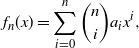
In this paper we study the persistence probability, i.e. the probability of not changing sign in the positive real line of the random polynomial
 $$
\begin{equation}
f_n(x)=\sum_{i=0}^{n} \binom{n}{i}a_ix^i,
\label{eqn1}
\end{equation}
$$
where the coefficients
 $a_i$
are real and independent and identically distributed (i.i.d.) standard normal random variables.
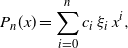
Our first motivation is from random polynomial theory in which the topic of the zeros of a random polynomial has been studied extensively since the seminal paper of Block and Pólya [3]. We review here relevant work on the persistence probability and refer the reader to standard monographs [2, 16] and recent articles [5, 10, 32, 35] and references therein for information on other aspects of random polynomials such as the expected number of roots, the central limit theorem, and large deviations. A random polynomial can be expressed generally by
 \begin{equation}
P_n(x)=\sum_{i=0}^{n} c_i\,\xi_i\,x^i,
\label{eqn2}
\end{equation}
where the
 $c_i$
are deterministic coefficients which may depend on both n and i, and the
 $\xi_i$
are random variables. The most popular random polynomials studied in the literature are:
(i) Kac polynomials (denoted by
 $P^{\rm K}_n$
):
${{c}_{i}}\text{:=1}$
,
(ii) Weyl (or flat) polynomials (
$P^{\rm W}_n$
):
${{c}_{i}}:=\frac{1}{i!}$
,(iii) Elliptic (or binomial) polynomials (
$P^{\rm E}_n$
):
$c_i\coloneqq\sqrt{\binom{n}{i}}$
.


For Kac polynomials, it is shown in [Reference Littlewood and Offord27, Reference Littlewood and Offord28] that when
 $\{\xi_i\}_{i=0}^n$
are i.i.d. and are either all uniform on
 $[-1, 1]$
, or all Gaussian or all uniform on
 $\{-1, 1\}$
,
 $\mathrm{P}(N^{\rm K}_{n}=0)=O(1/\log n)$
where
 $N^{\rm K}_n$
is the number of real zeros of the Kac polynomial
 $P_n^{\rm K}$
. This result is extended in [Reference Dembo, Poonen, Shao and Zeitouni9] to the case where the
 $\xi_i$
are i.i.d. random variables with the common distribution having finite moments of all orders as
 \[
\mathrm{P}(P^{\rm K}_n(x) > 0\ \text{for all}\ x\in{\mathbb{R}}) = n^{-4b_0+o(1)},
\]
where the constant
 $b_0$
is given by
 \[
b_0=-\lim\limits_{t\to\infty} t^{-1}\log\mathrm{P}(X_s>0\ %,~\forall
\text{for all}\ s\in[0,t]),\]
where X is a centered stationary Gaussian process with correlation
 \[\mathrm{E}(X_0X_t)=1/\cosh(t/2).\]
In [Reference Schehr and Majumdar33] the authors develop a mean-field approximation to rederive the persistence probability of (generalized) Kac polynomials, relating it to zero-crossing properties of the diffusion equation with random initial conditions. Moreover, using this method they predict and numerically verify the following asymptotic formulas for elliptic and Weyl models:
(i) For elliptic polynomials:
(3)where b is a positive constant defined as
\begin{equation}
\lim\limits_{n\rightarrow\infty}\frac{\log\mathrm{P}(P^{\rm E}_n(x)>0\ \ \text{for all}\ x\in{\mathbb{R}})}{\sqrt{n}}=-2\pi b,
\label{eqn3}
\end{equation}
(4)where Y(t) is a centered stationary Gaussian process with correlation
\begin{equation}
b=-\lim_{T\rightarrow\infty}\frac{\log\mathrm{P}(\inf_{0\leq t\leq T} Y(t))}{T},
\label{eqn4}
\end{equation}
$\mathrm{E}(Y_0Y_t)={\rm e}^{-t^2/2}$
.(ii) For Weyl polynomials:
(5)with the same constant b as in (4).
\begin{equation}
\lim\limits_{n\rightarrow\infty}\frac{\log\mathrm{P}(P^{\rm W}_n(x)>0\ %,~\forall
\text{for all}\ x\in{\mathbb{R}})}{\sqrt{n}}=-2 b,
\label{eqn5}
\end{equation}




The statement in (3) for elliptic polynomials is proven in [Reference Dembo and Mukherjee7]. In addition, this work also shows (5) for
 $I_n = [0,\sqrt{n}-\alpha_n]$
with
 $n^{-1/2}\alpha_n\rightarrow 0$
obtaining the persistence exponent
 $-b$
. More recently, by extending the method of [Reference Dembo and Mukherjee7], the authors of [Reference Can and Pham6] proved (5) for Weyl polynomials. Inspired by this development, in this paper we study the asymptotic behavior of the persistence probability in the positive real line of the random polynomial
 $f_n$
in (1). This is a new class of random polynomials and, as will be discussed in the next paragraph, the persistence probability of
 $f_{n-1}$
corresponds to the probability that an n-player two-strategy random evolutionary game has no internal equilibria.
Our second motivation comes from evolutionary game theory [Reference Hofbauer and Sigmund25, Reference Maynard Smith and Price31]. As will be shown in Appendix A, under certain assumptions the polynomial
 $f_n$
originates from the study of equilibrium points in random evolutionary game theory: finding an internal equilibrium point in a symmetric n-player two-strategy random game is equivalent to finding a positive zero of
 $f_{n-1}$
. In particular, the persistence probability of
 $f_{n-1}$
in the positive real line corresponds to the probability that the random game has no internal equilibria. Random evolutionary games have been used widely and successfully in the mathematical modelling of social and biological systems where limited information is available or where the environment changes so rapidly and frequently that one cannot predict the payoffs of their inhabitants. Such scenarios arise in fields such as biology, ecology, population genetics, economics, and social sciences [Reference Fudenberg and Harris17, Reference Gross, Rudolf, Levin and Dieckmann23, Reference Han, Traulsen and Gokhale24, Reference May30]. In these situations, due to randomness, characterizing the statistical properties of equilibrium points becomes essential and has attracted considerable interest in recent years. In [Reference Gokhale and Traulsen21, Reference Gokhale and Traulsen22, Reference Han, Traulsen and Gokhale24], the authors provide analytical and simulation results for random games with a small number of players (
 $n\leq 4$
) focusing on the probability of attaining the maximal number of equilibrium points. In [Reference Duong and Han11, Reference Duong and Han12, Reference Duong, Tran and Han14], the authors derive a closed formula for the expected number of internal equilibria, characterize its asymptotic behavior, and study the effect of correlations. Related work on the expected number of equilibrium points of large random complex systems arising from physics and ecology is presented in [Reference Fyodorov18, Reference Fyodorov and Khoruzhenko19, Reference Fyodorov and Nadal20]; see also references therein. More recently, [Reference Duong, Tran and Han13] offers, among other things, an analytical formula for the probability that a multi-player two-strategy game has a certain number of internal equilibria. Although the analytical formula is theoretically interesting, it involves complicated multiple integrals and is computationally intractable when the number of players becomes large. The present paper provides an asymptotic formula, as the number of players tends to infinity, for the probability that the game has no internal equilibria. Biologically this probability corresponds to the two extreme cases when the whole population consists of only one species/strategy while the other becomes extinct.
1.2. The main result of the paper
The main result of the present paper is the following theorem.
Theorem 1. Let
 $f_n$
be defined in (1) where the coefficients
 $a_i$
are i.i.d. standard normal random variables. Then we have
 \begin{equation}
\lim_{n \rightarrow \infty} \frac{\log {\mathrm{P}} (\,f_n(x) >0\ \ % , \, \forall
\text{for all}\ x\in (0,\infty))}{\pi \sqrt{n}}=-b,
\label{eqn6}
\end{equation}
where b is the persistence exponent defined by
 \begin{equation}
b= - \lim_{T \rightarrow \infty} \frac{\log {\mathrm{P}} (\inf_{0 \leq t \leq T} Z(t) >0)}{T} ,
\label{eqn7}
\end{equation}
where Z(t) is a centered stationary Gaussian process with correlation
 $\mathrm{E} (Z_0Z_t)={\rm e}^{-t^2/4}$
.
The idea of the proof is as follows. We first show that the contributions to the persistence exponent of the intervals
 $(0,n^{-1/6})$
and
 $(n^{1/6},\infty)$
are negligible. We then apply the method of [Reference Dembo and Mukherjee7] to prove that the main contribution from the interval
 $(n^{-1/6},n^{1/6})$
can be calculated approximately from that of a centered stationary Gaussian process with autocorrelation function
 $R(t)={\rm e}^{-t^2/4}$
.
1.3. Organization of the paper
The rest of paper is organized as follows. Section 2 contains technical lemmas. The proof of the main theorem is presented in Section 3. We provide further discussion on future work in Section 4. In Appendix A, we show the derivation of the random polynomial
 $f_n$
from the replicator dynamics for a symmetric multi-player two-strategy random evolutionary game.
2. Preliminaries
In this section we prove some technical results that will be used in the proof of the main theorem presented in Section 3.
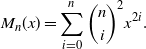
Since the
 $\{a_i\}$
are i.i.d. random variables of standard normal distribution, the random polynomial
 $f_n(x)$
is a Gaussian process with autocorrelation function
 \begin{equation*}
A_n(x,y)= \frac{M_n(\sqrt{xy})}{\sqrt{M_n(x)}\sqrt{M_n(y)}\,},
\end{equation*}
where
 \begin{equation}
M_n(x)=\sum \limits_{i=0}^{n} \binom{n}{i}^2x^{2i}.
\label{eqn8}
\end{equation}
We prove here a key lemma on the behavior of
 $M_n(x)$
as
 $n\rightarrow \infty$
.
Lemma 1. For
 $x\in (0,1]$
we define
 \[i_x=\left\lfloor \frac{nx}{x+1}\right\rfloor.\]
(i) For
 $\tfrac{\log n}{6n} \leq x \leq 1 $
we have
 \begin{eqnarray*}
\binom{n}{i_x}^2x^{2i_x} \leq M_n(x) \leq 3 i_x^{3/4} \binom{n}{i_x}^2x^{2i_x}.
\end{eqnarray*}
(ii) For
 $n^{-1/6} \leq x \leq 1 $
we have
 \begin{eqnarray*}
M_n(x)&=& (1+{O}(n^{-1/24})) \binom{n}{i_x}^2x^{2i_x}\frac{\sqrt{\pi n x}}{(x+1)}\\
&=&(1+{O}(n^{-1/24}))\frac{(x+1)^{2n+1}}{2\sqrt{\pi n x}}.
\end{eqnarray*}
Proof. The proof of this lemma is fairly lengthy and technical. The main idea is to use Stirling’s formula to approximate the summand in
 $M_n(x)$
by another function
 $J_x(\frac{i}{n})$
(see (9) below). The tasks are then to understand the behavior of
 $J_x(\frac{i}{n})$
, which is subtly dependent on the relationship between x and n. It turns out that the behavior of
 $M_n(x)$
depends on whether
 $x\in[\tfrac{\log n}{6n},1]$
or
 $x\in[n^{-1/6},1]$
as in parts (i)/(ii). This will be carried out using the intermediate parameter
 $i_x$
defined at the beginning of the lemma.
Let us start with Stirling’s formula that
 \begin{eqnarray*}
i! = \sqrt{2\pi i}(1+{O}(i^{-1})) \Big(\frac{i}{{\rm e}}\Big)^i.
\end{eqnarray*}
Therefore,
 \begin{eqnarray*}
\binom{n}{i}&=&\sqrt{\frac{n}{2\pi i(n-i)}} (1+{O}(\!\max(i^{-1},(n-i)^{-1}))) \bigg(\frac{n}{i}\bigg)^i \bigg(\frac{n}{n-i}\bigg)^{n-i}\\
&=& \sqrt{\frac{n}{2\pi i(n-i)}} (1+{O}(\!\max(i^{-1},(n-i)^{-1}))) \exp \bigg( n I\bigg(\frac{i}{n}\bigg) \bigg),
\end{eqnarray*}
where
 $I(0)=I(1)=0$
and, for
 $t\in(0,1)$
,
 \[I(t)=(t-1) \log (1-t)-t \log t.\]
Hence,
 \begin{eqnarray}
\binom{n}{i}^2 x^{2i} = \frac{n}{2\pi i(n-i)} (1+{O}(\!\max(i^{-1},(n-i)^{-1}))) \exp \bigg( 2n J_x\bigg(\frac{i}{n}\bigg) \bigg),
\label{eqn9}
\end{eqnarray}
where
 \[J_x(t)=I(t)+ t \log x.\]
We notice that
 $$
J_x\bigg(\frac{x}{x+1}\bigg)= \log (x+1), \quad J'_x\bigg(\frac{x}{x+1}\bigg)= 0, \quad J''_x(t)= \frac{-1}{t(1-t)}\ % \,\,\forall \,\,
\text{for all}\ t\in(0,1).
\label{eqn10}$$
Therefore, using the Taylor expansion we get
 \begin{align*}
J_x\bigg(\frac{i_x}{n}\bigg) &= J_x\bigg(\frac{x}{x+1}\bigg) + J_x'\bigg(\frac{x}{x+1}\bigg) \bigg( \frac{i_x}{n} -\frac{x}{x+1} \bigg) + \frac{J_x''(\eta_x)}{2} \bigg( \frac{i_x}{n} -\frac{x}{x+1} \bigg)^2\\
&= \log (x+1) + \frac{J_x''(\eta_x)}{2} \bigg( \frac{i_x}{n} -\frac{x}{x+1} \bigg)^2,
\end{align*}
with some
 $\eta_x \in ( \tfrac{i_x}{n}, \tfrac{x}{x+1})$
. Using the assumption that
 $x\in (0, 1]$
, we have
 \begin{eqnarray*}
\bigg | \frac{i_x}{n} - \frac{x}{x+1} \bigg | \leq \frac{1}{n}, \qquad |\,J''(\eta_x)| = \frac{1}{\eta_x(1-\eta_x)} \leq \frac{2n}{i_x}.
\end{eqnarray*}
Hence,
 \begin{eqnarray*}
2n\bigg(J_x\bigg(\frac{i_x}{n}\bigg) - \log(x+1) \bigg) \leq \frac{2}{i_x}.
\end{eqnarray*}
Therefore, using the fact that
 $\max(i_x^{-1},(n-i_x)^{-1})=i_x^{-1}$
, we get
 \begin{eqnarray}
\binom{n}{i_x}^2 x^{2i_x} &=& \frac{n}{2\pi i_x(n-i_x)} (1+{O}(i_x^{-1})) \exp \Big( 2n J_x\Big(\frac{i_x}{n}\Big) \Big) \label{eqn11}\end{eqnarray}
 \begin{eqnarray}
&=& \frac{ (x+1)^2}{2\pi n x}(1+{O}(i_x^{-1})) (x+1)^{2n} \notag\\
&=& (1+{O}(i_x^{-1}) )\frac{(x+1)^{2n+2}}{2 \pi nx}. \notag
\end{eqnarray}
We now estimate
 $M_n(x)$
. Observe that
 \begin{eqnarray*}
M_n(x) = \sum \limits_{i=0}^n \binom{n}{i}^2 x^{2i} = \binom{n}{i_x}^2 x^{2i_x} \sum \limits_{i=0}^n \frac{\binom{n}{i}^2 x^{2i}}{\binom{n}{i_x}^2 x^{2i_x}}.
\end{eqnarray*}
We notice that for any
 $i=0,\ldots,n$
,
 \begin{eqnarray*}
\binom{n}{i} \leq {\rm e}^{nI(i/n)}.
\end{eqnarray*}
Thus, for any
 $i=0,\ldots,n$
,
 \begin{eqnarray}
\binom{n}{i}^2 x^{2i} \leq {\rm e}^{2nJ_x(i/n)}.
\label{eqn12}
\end{eqnarray}
Observation O1. By (10), the function
 $J_x(t)$
is concave in (0,1) and attains a maximum at
 $t=\tfrac{x}{x+1}$
. Thus, for any closed interval
 $A\subset (0,1)$
,
 \begin{equation*}
\max \limits_{t \in A} J_x(t)= \max \limits_{t \in A_x} J_x(t),
\end{equation*}
with
 \[A_x=\bigg\{t\,:\, \bigg|t-\frac{x}{x+1}\bigg|=\min \limits_{s \in A} \bigg|s-\frac{x}{x+1}\bigg|\bigg\}.\]
Case 1:
 $i\leq i_x -i_x^{3/4}$
, or
 $i_x+ i_x^{3/4} \leq i \leq 60 i_x$
. Then, by (11), (12), and Observation O1, we have
 \begin{eqnarray*}
\frac{\binom{n}{i}^2 x^{2i}}{\binom{n}{i_x}^2 x^{2i_x}} &\leq & 4\pi i_x \exp \bigg( 2n \bigg[ J_x\bigg(\frac{i}{n}\bigg) -J_x\bigg(\frac{i_x}{n}\bigg) \bigg] \bigg) \notag \\
&\leq & 4\pi i_x \exp \bigg( 2n \bigg[ J_x\bigg(\frac{i_x \pm i_x^{3/4}}{n}\bigg) -J_x\bigg(\frac{i_x}{n}\bigg) \bigg] \bigg). \label{iix}
\end{eqnarray*}
By Taylor expansion,
 \begin{eqnarray*}
&&J_x\bigg(\frac{i_x \pm i_x^{3/4}}{n}\bigg) -J_x\bigg(\frac{i_x}{n}\bigg)=\pm \frac{i_x^{3/4}}{n} J'_x\bigg(\frac{i_x}{n}\bigg) + J''_x(\nu_x) \frac{i_x^{3/2}}{2n^2}\\[5pt]
&& \text{for some}\ \nu_x \in \bigg(\frac{i_x-i_x^{3/4}}{n},\frac{i_x+i_x^{3/4}}{n}\bigg).
\end{eqnarray*}
Notice that
 \begin{eqnarray}
\bigg |\,J'_x\bigg(\frac{i_x}{n}\bigg) \bigg |= \bigg |\,J'_x\bigg(\frac{i_x}{n}\bigg)-J'_x\bigg(\frac{x}{x+1}\bigg) \bigg | &\leq& \sup \limits_{y \in \big(\tfrac{i_x}{n}, \tfrac{x}{x+1}\big)} |\,J''(y)|\, \bigg |\frac{i_x}{n}-\frac{x}{x+1} \bigg | \notag \\
&\leq& \frac{4}{nx}
\label{eqn13}\end{eqnarray}
by using (10) and
 $\big|\tfrac{i_x}{n}-\tfrac{x}{x+1}\big|\leq \tfrac{1}{n}$
. On the other hand,
 \begin{eqnarray*}
J_x''(\nu_x)=\frac{-1}{\nu_x(1-\nu_x)} \leq \frac{-1}{\nu_x} \leq \frac{-n}{i_x+i_x^{3/4}} \leq \frac{-1}{2x}.
\end{eqnarray*}
Combining the above estimates, we get
 \begin{equation*}
\frac{\binom{n}{i}^2 x^{2i}}{\binom{n}{i_x}^2 x^{2i_x}} \leq 4\pi i_x \exp \bigg( \frac{8 i_x^{3/4}}{nx} - \frac{i_x^{3/2}}{2nx}\bigg) \leq 4\pi i_x \exp \bigg( - \frac{i_x^{3/2}}{4nx}\bigg) \leq 4\pi i_x {\rm e}^{-\tfrac{\sqrt{2nx}}{16}}.
\end{equation*}
Therefore, when nx is large enough,
 \begin{eqnarray}
M_{1,n}(x) &=& \sum \limits_{i\leq i_x -i_x^{3/4}} \frac{\binom{n}{i}^2 x^{2i}}{\binom{n}{i_x}^2 x^{2i_x}} + \sum \limits_{ i_x +i_x^{3/4} \leq i \leq 60 i_x} \frac{\binom{n}{i}^2 x^{2i}}{\binom{n}{i_x}^2 x^{2i_x}} \notag \\
&\leq& 61i_x \times 4\pi i_x {\rm e}^{-\tfrac{\sqrt{2nx}}{16}} \leq 244 \pi (nx)^2 {\rm e}^{-\tfrac{\sqrt{2nx}}{16}} \leq \frac{1}{nx}.
\label{eqn14}\end{eqnarray}
Case 2:
 $i>60i_x$
. Using the same arguments as in Case 1, we can show that
 \begin{eqnarray*}
\frac{\binom{n}{i}^2 x^{2i}}{\binom{n}{i_x}^2 x^{2i_x}} &\leq & 4\pi i_x \exp \bigg( 2n \bigg[ J_x\bigg(\frac{60i_x }{n}\bigg) -J_x\bigg(\frac{i_x}{n}\bigg) \bigg] \bigg)\\
&\leq& 4\pi i_x \exp \bigg( 2n \bigg[ \frac{4}{nx} \frac{59i_x}{n} - \frac{1}{120 i_x} \frac{(59i_x)^2}{2n^2} \bigg] \bigg) \\
&\leq & 4\pi i_x \exp \bigg(472 - \frac{59^2 nx}{240} \bigg)\\
&\leq & 4\pi i_x \exp \bigg(472 - \frac{59^2 \log n}{1440} \bigg) \leq 4 \pi i_x {\rm e}^{-12 \log n/5} = 4 \pi i_x n^{-12/5}.
\end{eqnarray*}
Notice that for the last line we assume that n is large enough and
 $nx \geq \log n/6$
. Therefore,
 \begin{eqnarray}
M_{2,n}(x) &=& \sum \limits_{ i \gt 60 i_x} \frac{\binom{n}{i}^2 x^{2i}}{\binom{n}{i_x}^2 x^{2i_x}} \leq n \times 4\pi i_x n^{-12/5} \leq n^{-1/5}.
\label{eqn15}
\end{eqnarray}
Case 3:
 $|i-i_x| \leq i_x^{3/4}$
. By (9), noting that in this case i and
 $i_x$
are of the same order of magnitude, we have
 \begin{eqnarray}
&& \frac{\binom{n}{i}^2 x^{2i}}{\binom{n}{i_x}^2 x^{2i_x}} = (1+{O}(i_x^{-1})) \frac{i_x(n-i_x)}{i(n-i)} \exp \bigg( 2n \bigg[ J_x\bigg(\frac{i}{n}\bigg) -J_x\bigg(\frac{i_x}{n}\bigg) \bigg] \bigg).
\label{eqn16}
\end{eqnarray}
Since
 $J_x(t)$
is a concave function,
 \begin{eqnarray}
J_x\bigg(\frac{i}{n}\bigg) -J_x\bigg(\frac{i_x}{n}\bigg) \leq J_x'\bigg(\frac{i_x}{n}\bigg) \frac{(i-i_x)}{n}.
\label{eqn17}
\end{eqnarray}
On the other hand, by (13),
 \begin{eqnarray}
\bigg|\,J_x'\bigg(\frac{i_x}{n}\bigg) (i-i_x)\bigg| \leq \frac{4|i-i_x|}{nx} \leq \frac{4 i^{3/4}_x}{nx} \leq \frac{4}{(i_x)^{1/4}}.
\label{eqn18}
\end{eqnarray}
We are now in a position to prove part (i). Indeed, from (16), (17), and (18), we have
 \begin{eqnarray*}
&& \frac{\binom{n}{i}^2 x^{2i}}{\binom{n}{i_x}^2 x^{2i_x}} \leq (1+i_x^{-1/2}) \frac{i_x(n-i_x)}{i(n-i)} \exp ( 8i_x^{-1/4} ) \leq (1+i_x^{-1/8}).
\end{eqnarray*}
Hence,
 \begin{eqnarray*}
&& 1\leq M_{3,n}(x) =\sum \limits_{|i-i_x| \leq i_x^{3/4}} \frac{\binom{n}{i}^2 x^{2i}}{\binom{n}{i_x}^2 x^{2i_x}} \leq 2i_x^{3/4} (1+i_x^{-1/8}).
\end{eqnarray*}
Combining this estimate with (14) and (15), we obtain part (i).
We now prove part (ii). Assume that
 $x\in(n^{-1/6},1)$
. Then, using (16) and Taylor expansion,
 $$
\frac{\binom{n}{i}^2 x^{2i}}{\binom{n}{i_x}^2 x^{2i_x}} & = (1+{O}(i_x^{-1})) \frac{i_x(n-i_x)}{i(n-i)} \exp \bigg( 2n \bigg[ J_x\bigg(\frac{i}{n}\bigg) -J_x\bigg(\frac{i_x}{n}\bigg) \bigg] \bigg)\\
&= (1+{O}(i_x^{-1/4})) \times \\
& \qquad \exp \bigg( 2n \bigg[ J_x'\bigg(\frac{i_x}{n}\bigg) \frac{(i-i_x)}{n}+ J_x''\bigg(\frac{i_x}{n}\bigg) \frac{(i-i_x)^2}{2n^2} + J_x'''(\nu_{i,x}) \frac{(i-i_x)^3}{6n^3} \bigg] \bigg),
$$
for some
 $\nu_{i,x} \in \big(\tfrac{i_x}{n}, \tfrac{i}{n}\big)$
.
We notice that
 $J_x'''(y) = {O}(y^{-2})\ \text{for all}~y\in \mathbb{R}$
. Therefore, by Taylor expansion,
 \begin{equation*}
J_x''\bigg(\frac{i_x}{n}\bigg)=J_x''\bigg(\frac{x}{x+1}\bigg) + {O}\bigg(\frac{1}{x^2}\bigg) \bigg(\frac{i_x}{n}-\frac{x}{x+1}\bigg) =J_x''\bigg(\frac{x}{x+1}\bigg) + {O}\bigg(\frac{1}{nx^2}\bigg),
\end{equation*}
and
 \begin{equation*}
J_x'''(\nu_{i,x})={O}\bigg(\frac{1}{x^2}\bigg).
\end{equation*}
Combining these estimates with (18), we get
 \begin{align*}
\frac{\binom{n}{i}^2 x^{2i}}{\binom{n}{i_x}^2 x^{2i_x}} &= (1+{O}(i_x^{-1/4})) \times \\
& \quad\ \exp \bigg( {O}(i_x^{-1/4}) + \bigg[ J_x''\bigg(\frac{x}{x+1}\bigg) + {O}\bigg(\frac{1}{nx^2}\bigg) + {O}\bigg( \frac{1}{x^2}\bigg) \bigg(\frac{i-i_x}{n}\bigg)\bigg]\frac{(i-i_x)^2}{n} \bigg) \\
&= (1+{O}(n^{-5/24})) \exp \bigg( \bigg[ J_x''\bigg(\frac{x}{x+1}\bigg) + {O}\bigg(n^{-1/24}\bigg)\bigg]\frac{(i-i_x)^2}{n} \bigg),
\end{align*}
since
 $x\in(n^{-1/6},1)$
and
 $|i-i_x|\leq i_x^{3/4} ={O}((nx)^{3/4})$
. Therefore, by using
 \[J_x''\bigg(\frac{x}{x+1}\bigg)=\frac{-(x+1)^2}{x}\]
and integral approximations, we can prove that
 \begin{eqnarray*}
M_{3,n}(x)&=& \sum \limits_{|i-i_x|\leq i_x^{3/4}} \frac{\binom{n}{i}^2 x^{2i}}{\binom{n}{i_x}^2 x^{2i_x}} \\
&=& (1+{O}(n^{-5/24})) \sum \limits_{|\,j|\leq i_x^{3/4}} \exp \bigg( \bigg[ \frac{-(x+1)^2}{x} +{O}(n^{-1/24}) \bigg] \frac{j^2}{n} \bigg)\\
&=& (1+{O}(n^{-5/24})) \sum \limits_{|\,j|\leq \big(\tfrac{nx}{x+1}\big)^{3/4}} \exp \bigg( - \bigg( j \frac{\sqrt{\tfrac{(x+1)^2}{x}+{O}(n^{-1/24})}}{\sqrt{n}} \bigg)^2 \bigg) \\
&=& (1+{O}(n^{-5/24})) \frac{\sqrt{n}}{\sqrt{\tfrac{(x+1)^2}{x}+{O}(n^{-1/24})}\,} \bigg( \int _{-\infty}^{\infty} {\rm e}^{-t^2}\,{\rm d} t + {O}({\rm e}^{-(nx)^{1/4}}) \bigg) \\
&=& (1+{O}(n^{-1/24})) \frac{\sqrt{\pi nx}}{x+1}.
\end{eqnarray*}
In conclusion, we have
 \begin{eqnarray*}
\sum \limits_{i=0}^n \binom{n}{i}^2 x^{2i} &=&\binom{n}{i_x}^2 x^{2i_x} (M_{1,n}(x)+M_{2,n}(x)+M_{3,n}(x)) \\
&=&(1+{O}(n^{-1/24})) \binom{n}{i_x}^2 x^{2i_x} \frac{\sqrt{\pi nx}}{x+1}\\
&=&(1+{O}(n^{-1/24})) \frac{(x+1)^{2n+1}}{2\sqrt{\pi nx}}.
\end{eqnarray*}
Part (ii) follows.
Remark 1. (Asymptotic behavior of
 $M_n$
via the Legendre polynomial.) The asymptotic formula of
 $M_n$
can also be calculated using Legendre polynomials, denoted by
 $L_n(x)$
, which are solutions to Legendre’s differential equation
 $$
\begin{equation*}
\frac{{\rm d}}{{\rm d}x}\bigg[(1-x^2)\frac{{\rm d}}{{\rm d}x}L_n(x)\bigg]+n(n+1)L_n(x)=0
\end{equation*}
$$
with initial data
 $L_0(x)=1$
,
 $L_1(x)=x$
. They have been used widely in physics and engineering and have many interesting properties; see [1] for more information. For instance,
 $L_n$
has the following explicit representation:
 $$
L_n(x)=\frac{1}{2^n}\sum_{i=0}^{n}
% \begin{pmatrix}
% n\\
% i
% \end{pmatrix}
\binom{n}{i}^2(x-1)^{n-i}(x+1)^i.
$$
According to [Reference Duong and Han12, Lemma 3], the polynomial
 $M_n$
defined in (8) and the Legendre polynomial
 $L_n$
satisfy the relation
 \begin{equation}
M_n(x)=(1-x^2)^n L_n\bigg(\frac{1+x^2}{1-x^2}\bigg).
\label{eqn19}
\end{equation}
According to [Reference Bender and Orszag1, Example 2, p.229] (see also [Reference Wang and Wong36]), the Legendre polynomial
 $L_n$
satisfies the following asymptotic behavior as
 $n\to\infty$
for any
 $x>1$
:
 \begin{equation}
L_n(x)\sim \frac{1}{\sqrt{2\pi n}}\frac{(x+\sqrt{x^2-1})^{n+\frac{1}{2}}}{(x^2-1)^{\frac{1}{4}}}\qquad\text{for}~ x>1.
\label{eqn20}
\end{equation}
From (19) and (20) we obtain the following asymptotic behavior for
 $M_n(x)$
as
 $n\to\infty$
for any
 $0<x<1$
:
 \begin{equation*}
M_n(x)\sim \frac{(x+1)^{2n+1}}{2 \sqrt{\pi n x}}.
\end{equation*}
This is the result obtained in part (ii) of Lemma 2. However, that part provided a stronger statement offering a quantitative estimate.
By transforming to
 $x=\tan^2(t/2\sqrt{n})$
,
 $y =\tan^2(s/2\sqrt{n})$
, we will show that for
 $x, y \in [n^{-1/6}, n^{1/6}]$
the autocorrelation
 $A_n(x,y)$
is close to
 ${\rm e}^{-(t-s)^2/4}$
. This means that the sequence of random polynomials
 $(\,f_n(x))$
converges weakly to the centered stationary Gaussian process Z(t) with covariance function
 $R(t)={\rm e}^{-t^2/4}$
. Then, by heuristic arguments, the persistence probability of
 $f_n$
should tend to the corresponding one of Z(t). To ensure the continuity of persistence exponents we need some restrictive conditions on the autocorrelation function. The following result, which is a combination of Theorem 1.6 in [7] and Lemma 3.1 in [8], gives us such conditions.
Lemma 2. Let
 ${\mathcal{S}}_{+}$
be the class of all nonnegative autocorrelation functions. Then the following statements hold:
(a) For a centered stationary Gaussian process
 $\{Z_t\}_{t\geq 0}$
of autocorrelation function
 $A(s, t) = A(0, t-s) \in {\mathcal{S}}_+$
, the nonnegative limit
 \[b(A)= - \lim_{T \rightarrow \infty} \frac{\log {\mathrm{P}} (\inf_{0 \leq t \leq T} Z(t) >0)}{T} \]
exists.
(b) Let
 $\{Z_t^{(k)}\}_{t\geq 0}$
,
 $1\leq k \leq \infty$
, be a sequence of centered Gaussian processes of unit variance and nonnegative autocorrelation functions
 $A_k(s,t)$
such that
 $A_{\infty}(s,t) \in {\mathcal{S}}_+$
. Assume that the following conditions hold:
(b1) We have
 $A_k(s,s+\tau)\rightarrow A_{\infty}(0,\tau)$
uniformly in
 $s\geq 0$
when
 $k \rightarrow \infty$
.
(b2) For some
 $\alpha >1$
,
 \begin{equation*}\label{con1}
\underset{k,\tau \rightarrow \infty}{\lim\sup} \ \underset{s\geq 0}{\sup} \bigg\{\tau^{\alpha}\log A_k(s,s+\tau) \bigg\} <-1.
\end{equation*}
(b3) There exists
 $\eta>1$
such that
 \begin{equation*}\label{con3}
\underset{u\downarrow 0}{\lim\sup}\,|\log u|^{\eta} \underset{1\leq k \leq \infty}{\sup}p_k^2(u)<\infty,
\end{equation*}
where
 $p_k^2(u)\coloneqq2-2\inf_{s\geq 0, \tau \in [0,u]}A_k(s,s+\tau)$
.
(b4) The function
 $A_{\infty}(0,\tau)$
is nonincreasing and satisfies, for any finite
 $h>0$
and
 $\theta\in (0,1)$
,
 \begin{equation*}\label{con4}
a^2_{h,\theta}=\underset{0<t\leq h}{\inf} \bigg\{ \frac{A_{\infty}(0,\theta t) -A_{\infty}(0,t)}{1-A_{\infty}(0,t)} \bigg\} >0.
\end{equation*}
Then we have
 $$
\underset{k,T \rightarrow \infty}{\lim} \frac{1}{T}\log {\mathrm{P}} (Z_t^{(k)}\gt0\ %,\, \forall
\text{for all}\ t\in [0,T] )=-b(A_{\infty}).
$$
While Lemma 2 shows the convergence of the persistence exponent of general Gaussian processes under strict conditions of autocorrelation functions, Lemma 3 below provides a lower bound on the persistence probability of a differentiable Gaussian process Z(t), assuming the simple condition that the variances of Z(t) and Z’(t) are comparable.
Lemma 3. [Reference Dembo and Mukherjee7, Lemma 4.1] There is a universal constant
 $\mu \in (0,1)$
such that the following statements hold:
(i) If
 $(Z_t)_{t \in [a,b]}$
is a differentiable centered Gaussian process satisfying
 \begin{equation*}
2(b-a)^2 \sup \limits_{t \in [a,b]} \mathrm{E} (Z_t'^2) \leq \sup \limits_{t \in [a,b]} \mathrm{E} (Z_t^2),
\end{equation*}
then
 \begin{equation*}
{\mathrm{P}} \Big( \inf_{t \in [a,b]} Z_t > 0 \Big) \geq \mu.
\end{equation*}
(ii) If
 $(Z_t)_{t \in [0, T]}$
is a differentiable centered Gaussian process with nonnegative autocorrelation function satisfying, for all
 $t \leq T$
,
 \begin{equation*}
2\Delta^2 \mathrm{E} (Z_t'^2) \leq \mathrm{E} (Z_t^2) %,
\end{equation*}
for some positive constant
 $\Delta$
, then
 \begin{equation*}
{\mathrm{P}} \Big( \inf_{t \in [0,T]} Z_t > 0 \Big) \geq \mu^{\big\lceil \frac{T}{\Delta}\big\rceil}.
\end{equation*}
Proof. Part (i) is exactly Lemma 4.1 in [Reference Dembo and Mukherjee7]. Part (ii) is a direct consequence of part (i). Indeed, we divide the interval [0, T] into
 $\big\lceil \tfrac{T}{\Delta}\big\rceil$
small intervals of length
 $\Delta$
. Then the condition of part (i) is verified in each small interval. Thus, using Slepian’s lemma and part (i), we get part (ii).
3. Proof of Theorem 1
In this section we prove the main theorem, Theorem 1, using the preliminary lemmas from Section 2. The proof consists of three steps. In Section 3.1 we show that the contribution to the persistence probability of the two intervals
 $(0,n^{-1/6})$
and
 $(n^{1/6},\infty)$
is negligible. Then in Section 3.2 we compute the persistence exponent from the main interval,
 $(n^{-1/6},n^{1/6})$
. Finally, by bringing the two previous steps together, we conclude the proof in Section 3.3.
3.1. Negligible intervals
We show here that the contribution of the intervals
 $(0,n^{-1/6})$
and
 $(n^{1/6},\infty)$
to the persistence exponent is negligible.
Proposition 1. We have:
(i)
$\lim \limits_{n\rightarrow \infty} \frac{1}{\sqrt{n} }\log {\mathrm{P}} (\,f_n(x)>0\ % \quad \forall
\text{for all}\ x \in (0, n^{-1/6})) =0$
,(ii)
$\lim \limits_{n\rightarrow \infty} \frac{1}{\sqrt{n} }\log {\mathrm{P}} (\,f_n(x)>0\ % \quad \forall
\text{for all}\ x \in (n^{1/6}, \infty)) =0$
.


Proof. Part (ii) is a consequence of part (i). Indeed, we have
 $$
{\mathrm{P}} (\,f_n(x)>0\ % \quad \forall
\text{for all}\ x \in (n^{1/6}, \infty)) = {\mathrm{P}} (\,f_n(x)>0\ % \quad \forall
\text{for all}\ x \in (0, n^{-1/6})),
$$
since, for
 $x\gt 0$
,
 \[f_n\bigg(\frac{1}{x}\bigg)=\frac{1}{x^n}\sum_{i=0}^{n} \binom{n}{i}a_ix^{n-i}\mathop{=}^{({\mathcal{L}})}\frac{f_n(x)}{x^n}. \]
Now it remains to prove part (i). Since the upper bound that
 \[\log {\mathrm{P}} (\,f_n(x)>0\ % \quad \forall
\text{for all}\ x \in (0,n^{-1/6})) \leq \log 1 =0\]
is trivial, we only need to show the lower bound,
 $$
\liminf \limits_{n \rightarrow \infty} \frac{1}{\sqrt{n} }\log {\mathrm{P}} (\,f_n(x)>0\ % \quad \forall
\text{for all}\ x \in (0,n^{-1/6})) \geq 0.
\label{eqn21}
$$
By Slepian’s lemma, (Reference Gokhale and Traulsen21) follows from the following lower bounds:
 $$
&& \liminf \limits_{n \rightarrow \infty} \frac{1}{\sqrt{n} }\log {\mathrm{P}} \big(\,f_n(x)\gt0\ \quad \forall
\text{for all}\ x \in \big(0,\tfrac{\log n}{6n}\big)\big) \geq 0, \label{eqn22}$$
 $$
&& \liminf \limits_{n \rightarrow \infty} \frac{1}{\sqrt{n} }\log {\mathrm{P}} \big(\,f_n(x)\gt0\ \quad \forall
\text{for all}\ x \in \big(\tfrac{\log n}{6n}, n^{-1/6}\big)\big) \geq 0.
\label{eqn23}$$
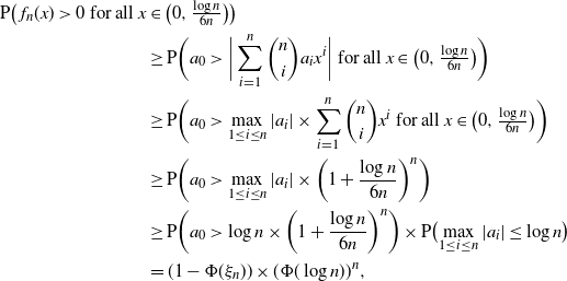
We first prove (Reference Gokhale and Traulsen22). We observe that
 $$
{\mathrm{P}} \big(\,f_n(x)>0\ % \quad \forall
\text{for all}\ x & \in \big(0,\tfrac{\log n}{6n}\big)\big) \notag \\
&\geq {\mathrm{P}} \bigg(a_0 > \bigg|\sum_{i=1}^{n} \binom{n}{i}a_ix^{i} \bigg|\ % \quad \forall
\text{for all}\ x \in \big(0,\tfrac{\log n}{6n}\big)\bigg) \notag \\
&\geq {\mathrm{P}} \bigg(a_0 > \max \limits_{1 \leq i \leq n} |a_i| \times \sum_{i=1}^{n} \binom{n}{i}x^{i}\ % \quad \forall
\text{for all}\ x \in \big(0,\tfrac{\log n}{6n}\big)\bigg) \notag \\
&\geq {\mathrm{P}} \bigg(a_0 > \max \limits_{1 \leq i \leq n} |a_i| \times \bigg(1+ \frac{\log n}{6n} \bigg)^n \bigg) \notag \\
&\geq {\mathrm{P}} \bigg(a_0 > \log n \times \bigg(1+ \frac{\log n}{6n} \bigg)^n \bigg) \times {\mathrm{P}} \big(\!\max \limits_{1 \leq i \leq n} |a_i| \leq \log n \big) \notag \\
&= (1-\Phi(\xi_n)) \times (\Phi(\log n))^n,
\label{eqn24}$$
where
 $\Phi(x)$
is the normal distribution function and
 \[\xi_n=\log n \times \bigg(1+ \frac{\log n}{6n} \bigg)^n.\]
We notice that
 $\log (1-\Phi(x))=(\tfrac{-1}{2}+o(1))x^2$
as
 $x\rightarrow \infty$
. Therefore, for n large enough,
 $$
(\Phi(\log n))^n \geq (1-{\rm e}^{-\log^2 n/4 } )^n \geq 1/2 %,
\label{eqn25}
$$
and
 \begin{eqnarray}
\liminf \limits_{n\rightarrow \infty}\frac{\log (1-\Phi(\xi_n))}{\sqrt{n}} \geq \liminf \limits_{n\rightarrow \infty} \frac{-\xi_n^2}{\sqrt{n}} \geq \liminf \limits_{n\rightarrow \infty} \frac{- \log^2 n \times {\rm e}^{\log n/3}}{\sqrt{n}} =0.
\label{eqn26}
\end{eqnarray}
Combining (24), (25), and (26), we get (22). We now prove (23). Let us define
 \[g_n(x)=(x+1)^{-n}f_n(x).\]
Then
 \begin{eqnarray*}
g_n'(x)&=&(x+1)^{-n} \bigg(\,f_n'(x)-\frac{n}{x+1}f_n(x) \bigg)\\
&=& (x+1)^{-n} \sum \limits_{i=0}^n \binom{n}{i} a_i x^i \bigg( \frac{i}{x}-\frac{n}{x+1}\bigg).
\end{eqnarray*}
Using Lemma 1, we have
 \begin{eqnarray}
\mathrm{E}(g_n(x)^2)=(x+1)^{-2n} M_n(x) \geq (x+1)^{-2n} \binom{n}{i_x}^2x^{2i_x},
\label{eqn27}
\end{eqnarray}
with
 \[i_x=\bigg\lfloor \frac{nx}{x+1}\bigg\rfloor.\]
Using the same arguments as in Lemma 1, we can also prove that
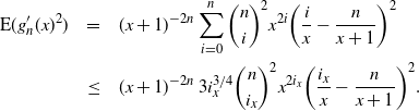 \begin{eqnarray}
\mathrm{E}(g_n'(x)^2) &=& (x+1)^{-2n} \sum \limits_{i=0}^n \binom{n}{i}^2 x^{2i} \bigg( \frac{i}{x}-\frac{n}{x+1}\bigg)^2 \notag\\
&\leq& (x+1)^{-2n} \, 3i_x^{3/4} \binom{n}{i_x}^2x^{2i_x}\bigg( \frac{i_x}{x}-\frac{n}{x+1}\bigg)^2.
\label{eqn28}\end{eqnarray}
Combining (27) and (28), we obtain
 \begin{eqnarray}
\mathrm{E}(g_n'(x)^2) \leq 3i_x^{3/4} \bigg( \frac{i_x}{x}-\frac{n}{x+1}\bigg)^2 \mathrm{E}(g_n(x)^2) \leq \frac{3n^{3/4}}{x^{5/4}} \mathrm{E}(g_n(x)^2).
\label{eqn29}
\end{eqnarray}
Thus, for
 $x\in \big(\tfrac{\log n}{6n},\tfrac{1}{\sqrt{n} }\big)$
,
 \begin{eqnarray*}
2 \Delta_{1,n}^2 \mathrm{E}(g_n'(x)^2) \leq \mathrm{E}(g_n(x)^2),
\end{eqnarray*}
with
 \[\Delta_{1,n}=\frac{(\log n) ^{5/8}}{8n}.\]
Applying Lemma 3, we have
 $$
{\mathrm{P}} \big(\,f_n(x)>0\ % \quad \forall
\text{for all}\ x \in \big(\tfrac{\log n}{6n},\tfrac{1}{\sqrt{n}}\big)\big) & = {\mathrm{P}} \big(g_n(x)>0\ % \quad \forall
\text{for all}\ x \in \big(\tfrac{\log n}{6n},\tfrac{1}{\sqrt{n}}\big)\big) \\
& \geq \mu^{\frac{1}{\Delta_{1,n} \sqrt{n}}}.
$$
Therefore,
 $$
\liminf \limits_{n\rightarrow \infty}\frac{1}{\sqrt{n}} \log {\mathrm{P}} \big(\,f_n(x)>0\ % \quad \forall
\text{for all}\ x \in \big(\tfrac{\log n}{6n},\tfrac{1}{\sqrt{n}}\big)\big) \geq \liminf \limits_{n\rightarrow \infty} \frac{\log \mu}{n \Delta_{1,n}} =0.
\label{eqn30}
$$
Using (29) for
 $x \in (n^{-1/2},n^{-1/6})$
, we get
 $$
2 \Delta_{2,n}^2 \mathrm{E}(g_n'(x)^2) \leq \mathrm{E}(g_n(x)^2) %,
$$
with
 \[\Delta_{2,n}=\frac{1}{3n^{11/16}}.\]
Applying Lemma 3, we have
 $$
{\mathrm{P}} (\,f_n(x)\gt0\ % \quad \forall
\text{for all}\ x \in (n^{-1/2},n^{-1/6})) & = {\mathrm{P}} (g_n(x)\gt0\ % \quad \forall
\text{for all}\ x \in (n^{-1/2},n^{-1/6}) ) \\
& \geq \mu^{\frac{1}{n^{1/6}\Delta_{2,n} }}.
$$
Therefore,
 $$
\liminf \limits_{n\rightarrow \infty}\frac{1}{\sqrt{n}} \log {\mathrm{P}} (\,f_n(x)\gt0\ % \quad \forall
\text{for all}\ x \in (n^{-1/2},n^{-1/6}) ) \geq \liminf \limits_{n\rightarrow \infty} \frac{\log \mu}{n^{2/3} \Delta_{2,n}} =0.
\label{eqn31}
$$
3.2. The main interval
We make the transformation
 \[x=\tan^2\bigg(\frac{t}{2\sqrt{n}} \bigg).\]
Then
 $x\in(n^{-1/6},n^{1/6})$
is equivalent to
 $t\in (\alpha_n, \pi\sqrt{n}-\alpha_n)$
, with
 \[\alpha_n=2 \sqrt{n} \tan^{-1}(n^{-1/12})=(2+o(1))n^{5/12}.\]
Let us define, for
 $t \in (\alpha_n, \pi\sqrt{n}-\alpha_n)$
,
 \[h_n(t)=f_n(\tan^2(t/2\sqrt{n})).\]
Then
 $$
{\mathrm{P}} ( f_n(x) >0\ % \quad \forall
\text{for all}\ x \in (n^{-1/6},n^{1/6}) ) = {\mathrm{P}} ( h_n(t) >0\ % \quad \forall
\text{for all}\ t \in (\alpha_n, \pi\sqrt{n}-\alpha_n)).
$$
Moreover, the autocorrelation function of
 $h_n(t)$
is
 \begin{eqnarray*}
B_n(t,s)= A_n \big( \tan^2\big(\tfrac{t}{2 \sqrt{n}}\big), \tan^2\big( \tfrac{s}{2 \sqrt{n}} \big)\big) = \frac{M_n \big(\tan\big(\tfrac{t}{2 \sqrt{n}}\big) \tan\big( \tfrac{s}{2 \sqrt{n}} \big) \big)}{\sqrt{M_n\big(\tan^2\big(\tfrac{t}{2 \sqrt{n}}\big)\big)} \sqrt{M_n\big(\tan^2\big(\tfrac{s}{2 \sqrt{n}}\big)\big)}\,}.
\end{eqnarray*}
We recall the approximation on
 $M_n(u)$
.
For
 $u\in(n^{-1/6},1)$
,
 \begin{equation}
M_n(u)=(1+O(n^{-1/24}))\frac{(u+1)^{2n+1}}{\sqrt{\pi n u}}.
\label{eqn32}
\end{equation}
For
 $u \in (1, \infty)$
, we remark that
 \[M_n(u) = u^{2n} M_n\big(\tfrac{1}{u}\big).\]
Therefore, the estimate (32) holds for all
 $u\in (n^{-1/6},n^{1/6})$
. Hence,
 \begin{eqnarray*}
B_n(t,s) &=& \frac{M_n \big(\tan\big(\tfrac{t}{2 \sqrt{n}}\big) \tan\big( \tfrac{s}{2 \sqrt{n}} \big) \big)}{\sqrt{M_n\big(\tan^2\big(\tfrac{t}{2 \sqrt{n}}\big)\big)} \sqrt{M_n\big(\tan^2\big(\tfrac{s}{2 \sqrt{n}}\big)\big)}\,} \\
&=& (1+O(n^{-1/24}))\bigg( \frac{\big(1+ \tan\big(\tfrac{t}{2 \sqrt{n}}\big) \tan\big( \tfrac{s}{2 \sqrt{n}} \big)\big)^2}{ \big(1+\tan^2\big(\tfrac{t}{2 \sqrt{n}}\big) \big)\big(1+\tan^2\big(\tfrac{s}{2 \sqrt{n}}\big) \big)}\bigg)^{\tfrac{2n+1}{2}}\\
&=&(1+O(n^{-1/24})) \bigg[ \cos \bigg(\frac{t-s}{2\sqrt{n}} \bigg)\bigg]^{2n+1}.
\end{eqnarray*}
We shift the interval
 $(\alpha_n, \pi \sqrt{n} -\alpha_n)$
to the interval
 $(0,\pi \sqrt{n}-2 \alpha_n)$
by changing variable to
 $u=t-\alpha_n$
, and define
 \[\bar{h}_n(u)=h_n(u+\alpha_n).\]
Then the autocorrelation of
 $\bar{h}_n(u)$
is
 \begin{eqnarray}
\bar{B}_n(u,v) = B_n(u+ \alpha_n, v+\alpha_n) = (1+O(n^{-1/24})) \bigg[ \cos \bigg(\frac{u-v}{2\sqrt{n}} \bigg)\bigg]^{2n+1}.
\label{eqn33}
\end{eqnarray}
Observe that, for fixed u,v,
 \begin{eqnarray*}
\bar{B}_n(u,v) \rightarrow {\rm e}^{-(u-v)^2/4}.
\end{eqnarray*}
This fact suggests verifying conditions (b1)–(b4) of Lemma 2 for the sequence of Gaussian processes
 $\{Z_t^{(n)}\}$
with autocorrelation functions
 $\bar{B}_n(u,v)$
and the limit stationary Gaussian process
 $Z_t^{(\infty)}$
with autocorrelation function
 ${\rm e}^{-(u-v)^2/4}$
.
Verification of condition (b1). This is easily deduced from (33).
Verification of condition (b2). Here we consider two cases. In the first case, where
 $\tau/\sqrt{n} \rightarrow 0$
as
 $\tau, n \rightarrow \infty$
,
 \begin{eqnarray*}
\tau^{\alpha} \bar{B}_n(u,u+\tau) \leq ({\rm const}) \tau^{\alpha} \bigg[ \cos \bigg(\frac{\tau}{2\sqrt{n}} \bigg)\bigg]^{2n+1} \leq ({\rm const}) \tau^{\alpha} {\rm e}^{-\tau^2/4} \rightarrow 0.
\end{eqnarray*}
In the second case, assume that there exists a positive constant
 $c_0$
such that
 $\tau/\sqrt{n} \geq c_0$
; then, as
 $\tau, n \rightarrow \infty$
,
 \begin{eqnarray*}
\tau^{\alpha} \bar{B}_n(u,u+\tau) \leq ({\rm const}) n^{\alpha/2} \bigg[ \cos \bigg(c_0/2 \bigg)\bigg]^{2n+1} \rightarrow 0.
\end{eqnarray*}
Thus condition (b2) is verified.
Verification of condition (b3). Using (33), we have, for n large enough,
 \begin{eqnarray*}
\bar{B}_n(t,t+\tau) \geq (1-n^{-1/30}) \bigg[\cos \bigg( \frac{\tau}{2 \sqrt{n}}\bigg)\bigg] ^{2n+1} \geq (1-n^{-1/30})(1-\tau^2).
\end{eqnarray*}
Therefore,
 \begin{eqnarray*}
\bar{p}^2_n(w) = 2 -2 \inf_{\substack{0\leq \tau\leq w \\ 0\leq t, t + \tau \leq \pi \sqrt{n} -2 \alpha_n}} \bar{B}_n(t, t+ \tau) \leq 2 w^2 + 2 n^{-1/30}.
\end{eqnarray*}
Hence, for any
 $\delta >0$
, as
 $w\rightarrow 0$
,
 \begin{eqnarray*}
|\log w|^2\sup \limits_{n \geq w^{-\delta}} \bar{p}_n^2(w) \rightarrow 0.
\end{eqnarray*}
Thus, to verify condition (b3) it suffices to show that, for some
 $\delta >0$
,
 \begin{eqnarray}
\lim \limits_{w \rightarrow 0^+}|\log w|^2\sup \limits_{n \leq w^{-\delta}} \bar{p}_n^2(w) < \infty.
\label{eqn34}
\end{eqnarray}
To show that (34) holds, it is sufficient to prove that
 \begin{eqnarray}
\lim \limits_{u \rightarrow 0^+}|\log u|^2\sup \limits_{n \leq u^{-\delta}} p_n^2(u) < \infty,
\label{eqn35}
\end{eqnarray}
where
 \begin{eqnarray*}
p^2_n(u) = 2 -2 \inf_{{\substack{0\leq y-x \leq u \\n^{-1/6} \leq x \leq y \leq n^{1/6} }}} A_n(x, y).
\end{eqnarray*}
Recall that
 \begin{eqnarray*}
A_n(x,y)= \frac{M_n(\sqrt{xy})}{\sqrt{M_n(x)}\sqrt{M_n(y)}\,},
\end{eqnarray*}
where
 \[M_n(x)=\sum \limits_{i=0}^n \binom{n}{i}^2x^{2i}.\]
We have
 \begin{eqnarray*}
\varepsilon_n(x,y)\coloneqq M_n(\sqrt{xy}) - M_n(x)= \sum \limits_{i=0}^n \binom{n}{i}^2x^{i}(y^i-x^i) \geq 0,
\end{eqnarray*}
since
 $y\geq x$
, and
 \begin{eqnarray*}
\tilde{\varepsilon}_n(x,y)\coloneqq M_n(y) - M_n(x)- 2 \varepsilon_n(x,y) =\sum \limits_{i=0}^n \binom{n}{i}^2(y^i-x^i)^2 \geq 0.
\end{eqnarray*}
Let
 $a >0 $
and
 $b,c \geq 0$
be real numbers satisfying
 $ac-b^2 \geq 0$
. Then
 \begin{eqnarray*}
1-\frac{a+b}{\sqrt{a(a+2b+c)}\,} = \frac{ac-b^2}{\big(a+b+\sqrt{a(a+2b+c)}\big)\sqrt{a(a+2b+c)}\,}\leq \frac{ac-b^2}{a^2}.
\end{eqnarray*}
By the Cauchy–Schwarz inequality,
 $M_n(x)\tilde{\varepsilon}_n(x,y)-\varepsilon^2_n(x,y)\geq 0$
. Hence, using the above inequality for
 $a=M_n(x)$
,
 $b=\varepsilon_n(x,y)$
, and
 $c=\tilde{\varepsilon}_n(x,y)$
, we get
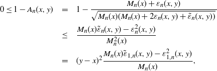 \begin{eqnarray}
0 \leq 1- A_n(x,y) &=& 1- \frac{M_n(x)+\varepsilon_n(x,y)}{\sqrt{M_n(x)( M_n(x)+ 2 \varepsilon_n(x,y) + \tilde{\varepsilon}_n(x,y))}\,} \notag\\
&\leq& \frac{M_n(x) \tilde{\varepsilon}_n(x,y) -\varepsilon_n^2(x,y)}{M_n^2(x)} \notag \\
&=& (y-x)^2 \frac{M_n(x) \tilde{\varepsilon}_{1,n}(x,y) -\varepsilon_{1,n}^2(x,y)}{M_n(x)},
\label{eqn36}\end{eqnarray}
with
 $$
\varepsilon_{1,n}(x,y) =\sum \limits_{i=0}^n \binom{n}{i}^2x^{i} \bigg(\frac{y^i-x^i}{y-x}\bigg) %,
$$
and
 \begin{eqnarray*}
\tilde{\varepsilon}_{1,n}(x,y) =\sum \limits_{i=0}^n \binom{n}{i}^2 \bigg(\frac{y^i-x^i}{y-x}\bigg)^2.
\end{eqnarray*}
Using the fact that
 \begin{eqnarray*}
\sum \limits_{i=0}^n a_i^2 \sum \limits_{i=0}^n b_i^2 - \bigg(\sum \limits_{i=0}^n a_i b_i \bigg)^2= \sum \limits_{i<j}^n (a_ib_j-a_jb_i)^2,
\end{eqnarray*}
we get
 \begin{eqnarray}
M_n(x) \tilde{\varepsilon}_{1,n}(x,y) -\varepsilon_{1,n}^2(x,y) = \sum_{i<j} \binom{n}{i}^2 \binom{n}{j}^2x^{2i}y^{2i}\bigg(\frac{y^{j-i}-x^{j-i}}{y-x}\bigg)^2.
\label{eqn37}
\end{eqnarray}
We notice that
 $$
\begin{eqnarray}
0\leq y-x \leq \tau \leq u, %
\qquad n\leq u^{-\delta}, %
\qquad x \geq n^{-1/6} \geq u^{\delta/6}.
\label{eqn38}
\end{eqnarray}
$$
Hence,
 $$
\begin{eqnarray}
y^{2i}\leq(x+u)^{2i}=x^{2i} \bigg(1+\frac{u}{x}\bigg)^{2i} \leq x^{2i}\bigg(1+n^{\tfrac{1}{6} -\tfrac{1}{\delta}}\bigg)^{2n} \leq 2 x^{2i} %,
\label{eqn39}
\end{eqnarray}
$$
for all
 $\delta \leq 1/2$
and n large enough. Moreover, since
 $y-x \leq u \leq x$
,
 \begin{eqnarray}
\frac{y^{j-i}-x^{j-i}}{y-x}=\sum_{k=0}^{j-i-1}(y-x)^kx^{j-i-k} \leq (j-i)x^{j-i-1} \leq nx^{j-i-1}.
\label{eqn40}
\end{eqnarray}
Combining (37), (39), and (40) yields that
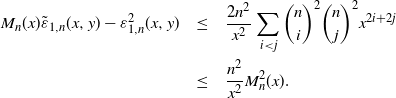 \begin{eqnarray}
M_n(x) \tilde{\varepsilon}_{1,n}(x,y) -\varepsilon_{1,n}^2(x,y) &\leq& \frac{2n^2}{x^2}\sum_{i<j} \binom{n}{i}^2 \binom{n}{j}^2x^{2i+2j} \notag\\
&\leq& \frac{n^2}{x^2}M_n^2(x).
\label{eqn41}\end{eqnarray}
It follows from (36), (38), and (41) that
 $$
\begin{equation*}
0\leq 1-A_n(x,y) \leq \frac{u^2n^2}{x^2} \leq u^{2-7\delta/3} \leq u^{5/6} %,
\end{equation*}
$$
for
 $\delta \leq 1/2$
. As consequence, (35) holds.
Verification of condition (b4). This is easy to check (or see Remark 3.1 in [26]).
By the validity of conditions (b1)–(b4), we deduce from Lemma 2 the following proposition.
Proposition 2. We have
 \[ \lim \limits_{n\rightarrow \infty} \frac{1}{\pi \sqrt{n} }\log {\mathrm{P}} (\,f_n(x)>0\ % \quad \forall
\text{for all}\ x \in ( n^{-1/6},n^{1/6})) = -b, \]
with b as in Theorem 1.
3.3. Conclusion
Thanks to Slepian’s inequality, using Propositions 1 and 2 we get
 \[ \liminf \limits_{n\rightarrow \infty} \frac{1}{ \pi \sqrt{n} }\log {\mathrm{P}} (\,f_n(x)>0\ % \quad \forall
\text{for all}\ x \in (-\infty, \infty)) \geq -b. \]
On the other hand, it follows directly from Proposition 2 that
 \[ \limsup \limits_{n\rightarrow \infty} \frac{1}{ \pi \sqrt{n} }\log {\mathrm{P}} (\,f_n(x)>0\ % \quad \forall
\text{for all}\ x \in (-\infty, \infty)) \leq -b. \]
Combining these two inequalities, we get Theorem 1.
4. Summary and future work
We have obtained an asymptotic formula for the persistence probability of the random polynomial
 $f_n$
in (1) that arises from evolutionary game theory. The persistence probability corresponds to the probability that a symmetric n-player two-strategy random game has no internal equilibria. We note that
 $f_n$
forms a different class of random polynomials that have been studied extensively in the literature, particularly in random polynomial theory; see [Reference Edelman and Kostlan15] and the recent paper [Reference Lubinsky, Pritsker and Xie29], and references therein, for information. There are several open problems that are of interest for both evolutionary game theory and random polynomial theory that we do not address in this paper, such as proving a central limit theorem and a large deviation principle for the empirical measures of the real zeros of
 $f_n$
, as well as studying universality phenomena for this class of random polynomials. We leave these problems for future research.
Appendix A
Derivation of
 $f_n$
from evolutionary game theory
In this appendix we review the derivation of the random polynomial
 $f_n$
in (1) from the replicator dynamics for multi-player two-strategy games in evolutionary game theory. The replicator equation for multi-player two-strategy games has already been derived in previous works [Reference Gokhale and Traulsen21, Reference Hofbauer and Sigmund25, Reference Sigmund34]. For the sake of completeness, we rederive it here.
We consider an infinitely large population consisting of individuals using two strategies, A and B. Let y,
 $0 \leq y\leq 1$
, be the frequency of strategy A in the population. The frequency of strategy B is thus
 $(1-y)$
. The interaction of the individuals in the population is in randomly selected groups of n participants; that is, they interact and obtain their fitness from n-player games. In this paper we consider symmetric games where the payoffs do not depend on the ordering of the players. Let
 $a_k$
(respectively,
 $b_k$
) be the payoff that an A (respectively, B) strategist achieves when interacting with a group containing k A strategists (and
 $n-k$
B strategists). In symmetric games, the probability that an A strategist interacts with k other A strategists in a group of size n is
 $$
\begin{equation*}
% \begin{pmatrix}
% n-1\\
% k
% \end{pmatrix}
\binom{n-1}{k}y^k (1-y)^{n-1-k}.
\end{equation*}
$$
We note that this probability depends only on the number k of A strategists but not on the particular order of the group. The average payoffs of A and B are, respectively,
 $$
\begin{equation*}
\pi_A= \sum\limits_{k=0}^{n-1}a_k
% \begin{pmatrix}
% n-1\\
% k
% \end{pmatrix}
\binom{n-1}{k}y^k (1-y)^{n-1-k}, \quad
\pi_B = \sum\limits_{k=0}^{n-1}b_k
% \begin{pmatrix}
% n-1\\
% k
% \end{pmatrix}
\binom{n-1}{k}y^k (1-y)^{n-1-k}.
\end{equation*}
$$
The replicator equation of a d-player two-strategy game is given by [Reference Gokhale and Traulsen21, Reference Hofbauer and Sigmund25, Reference Sigmund34]
 \begin{equation*}
\dot{y}=y(\pi_A-\overline{\pi})=y(1-y)(\pi_A-\pi_B),
\end{equation*}
where
 $\overline{\pi}\coloneqq y\pi_A+(1-y)\pi_B$
is the average payoff of the population. The replicator equation reflects natural selection. In fact, if
 $\pi_A\geq \overline{\pi}$
then y increases, that is A spreads in the population; similarly, if
 $\pi_A\lt\overline{\pi}$
then y decreases and A declines. Equilibrium points of the dynamics satisfy
 $y(1-y)(\pi_A-\pi_B)=0$
. Since
 $y=0$
and
 $y=1$
are two trivial equilibrium points, we focus only on internal ones, i.e.
 $0 \lt y \lt 1$
. They satisfy the condition that the fitnesses of both strategies are the same,
 $\pi_A=\pi_B$
, which gives rise to
 $$
\begin{equation*}
\sum\limits_{k=0}^{n-1}\beta_k
% \begin{pmatrix}
% d-1\\
% k
% \end{pmatrix}
\binom{d-1}{k}y^k (1-y)^{n-1-k} = 0,
\end{equation*}
$$
where
 $\beta_k = a_k - b_k$
. Using the transformation
 $x= \frac{y}{1-y}$
, with
 $0\lt x \lt +\infty$
, and dividing the left-hand side of the above equation by
 $(1-y)^{n-1}$
, we obtain the following polynomial equation for x:
 $$
\begin{equation}
\sum\limits_{k=0}^{n-1}\beta_k
% \begin{pmatrix}
% n-1\\
% k
% \end{pmatrix}
\binom{n-1}{k}x^k=0.
\label{eqn42}
\end{equation}
$$
Note that this equation can also be derived from the definition of an evolutionary stable strategy; see, e.g., [Reference Broom, Cannings and Vickers4]. In large complex systems, information about the interaction between participants is rarely available at a level of detail sufficient for the exact computation of the payoff matrix; therefore, it is necessary to suppose that the payoff matrix entries
 $a_k$
and
 $b_k$
(thus
 $\beta_k$
) for
 $0\leq k\leq n-1 $
are random variables. We then obtain random games and the expression on the right-hand side of (42) becomes a random polynomial. It is exactly the random polynomial
 $f_{n-1}$
in (1) that we started with.
We note that in this paper we needed to make the assumption that the payoff differences
 $a_k-b_k$
are independent standard normal random variables. This choice could be interpreted as modeling noise added to the payoffs of a game where both strategies are neutral, i.e. always have identical payoffs. Although this assumption is rather restricted, it provides an exact match between evolutionary game theory and random polynomial theory which opens up a new avenue for future research to, among other things, relax the identical and independent assumption.
Acknowledgements
The first author is supported by the fellowship of the Japan Society for the Promotion of Science and the Grant-in-Aid for JSPS fellows Number 17F17319. We would like to thank the anonymous referees for their useful suggestions.


