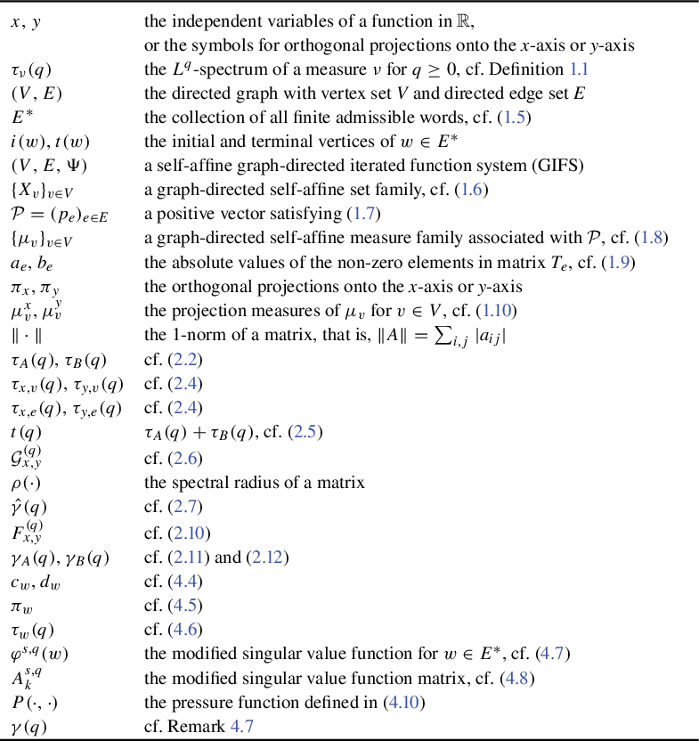
1 Introduction
Let
 $\{T_1, \ldots , T_N\}$
be a finite collection of affine contracting non-singular matrices and let
 $\Psi =\{\psi _i(\cdot )=T_i(\cdot )+t_i\}_{i=1}^N$
be an iterated function system (IFS) with
 $t_i\in \mathbb {R}^n$
for all
 $i\in \{1,\ldots , N\}$
. It is well known that there exists a unique non-empty compact set X such that
 $$ \begin{align*} X=\bigcup_{i=1}^N \psi_i(X). \end{align*} $$
We call
 $\Psi $
a self-affine IFS and X a self-affine set. In the special case when all the maps
 $\psi _i$
are contracting similitudes, call
 $\Psi $
a self-similar IFS and X a self-similar set.
For a positive probability vector
 $\mathcal {P}=(p_i)_{i=1}^N$
, there exists a probability measure
 $\mu $
satisfying
 $$ \begin{align*} \mu= \sum_{i=1}^N p_i \cdot \mu\circ \psi_i^{-1}. \end{align*} $$
Call
 $\mu $
a self-affine measure (respectively self-similar measure) when
 $\Psi $
is a self-affine IFS (respectively self-similar IFS).
The dimension theory of self-affine sets or measures is one of the central problems in fractal geometry. Historically, there are two basic strands to determine the Hausdorff and box dimensions of self-affine sets. The first strand, pioneered by Falconer’s seminal work [Reference Falconer9] on generic self-affine sets, revolves around the concept of the affinity dimension
 $d(T_1,\ldots ,T_N)$
. This dimension, defined in terms of the singular value functions of the linear parts
 $\{T_1,\ldots ,T_N\}$
, was shown to be the value of the Hausdorff and box dimensions for almost sure translation:
 $$ \begin{align*} \dim_H X=\dim_B X=d(T_1,\ldots, T_N) \text{ for Lebesgue-almost sure } \mathfrak{t}=(t_1, \ldots, t_N)\in \mathbb{R}^{nN}. \end{align*} $$
Falconer’s original proof required the linear part
 $T_i$
to have norms less than
 $1/3$
, which was later improved by Solomyak [Reference Solomyak50] to
 $1/2$
and the constant
 $1/2$
is proven to be sharp in [Reference Edgar8, Reference Solomyak50]. Along this direction, the study is thriving, encompassing both further developments of the generic theory and the pursuit of deterministic criteria under which a self-affine set attains the affinity dimension, that is,
 $\dim _H X =d(T_1,\ldots ,T_N)$
. This extensive body of literature includes, for example, [Reference Bárány, Hochman and Rapaport2, Reference Bochi and Morris4, Reference Falconer and Kempton12, Reference Feng and Shmerkin18, Reference Käenmäki25, Reference Morris38, Reference Morris and Shmerkin40] and the references therein.
The other strand of study is to focus on special classes of self-affine sets that are notable for having distinct Hausdorff and box dimensions. The investigation of such sets was pioneered by McMullen [Reference McMullen36] and Bedford [Reference Bedford3], who considered planar box-like self-affine sets with homogeneous grid structure. Their approaches were further developed by Lalley and Gatzouras [Reference Lalley and Gatzouras31] and Barański [Reference Barański1] to box-like sets with certain geometric arrangement or general grid structure. See [Reference Das and Simmons7, Reference Fraser and Jurga22, Reference Kenyon and Peres28, Reference Kolossváry30] for extensions to higher dimensions.
The planar box-like self-affine sets without grid structure were first considered by Feng and Wang [Reference Feng and Wang19], and later extended by Fraser [Reference Fraser20, Reference Fraser21], who allowed the IFSs to have non-trivial rotations and reflections, that is, the linear parts of maps were allowed to be diagonal or anti-diagonal. All these works [Reference Feng and Wang19–Reference Fraser21] on box-like self-affine sets focus on computing the
 $L^q$
-spectra of their associated self-affine measures. See also [Reference Falconer, Fraser and Lee11] for an extension to non-conformal measures.
In this paper, we continue to study the
 $L^q$
-spectra of self-affine measures. Let
 $\nu $
be a compactly supported Borel probability measure on
 $\mathbb {R}^n$
with
 $n\geq 1$
. For
 $\delta>0$
, let
 $\mathcal {M}_\delta $
be the collection of closed cubes in the
 $\delta $
-mesh of
 $\mathbb {R}^n$
. For
 $q\geq 0$
, write
 $$ \begin{align*} \mathcal{D}_\delta^q(\nu)=\sum_{Q\in \mathcal{M}_\delta}\nu(Q)^q. \end{align*} $$
Definition 1.1. For
 $q\geq 0$
, the upper and lower
 $L^q$
-spectra of
 $\nu $
are defined to be
 $$ \begin{align*} \overline{\tau}_\nu(q)=\limsup_{\delta\to 0+}\frac{\log \mathcal{D}_\delta^q(\nu)}{-\log \delta} \end{align*} $$
and
 $$ \begin{align*}\underline{\tau}_\nu(q)=\liminf_{\delta\to 0+}\frac{\log \mathcal{D}_\delta^q(\nu)}{-\log \delta}, \end{align*} $$
respectively. If these two values coincide, we define the
 $L^q$
-spectra of
 $\nu $
to be their common value and denote it as
 $\tau _\nu (q)$
.
It is known that as functions of q, both
 $\underline {\tau }_\nu (q),\overline {\tau }_\nu (q)$
are decreasing and equal to zero at
 $q=1$
. Also, they are convex, continuous on
 $(0,\infty )$
, and Lipschitz on
 $[\unicode{x3bb} ,\infty )$
for any
 $\unicode{x3bb}>0$
. Note that when
 $q=0$
, the upper and lower
 $L^q$
-spectra are equal to the upper and lower box dimensions of
 $\text {supp}\nu $
(the support of
 $\nu $
), respectively. Another important property of
 $L^q$
-spectra is that if it is differential at
 $q=1$
, then the measure
 $\nu $
is exact dimensional and the Hausdorff dimension of
 $\nu $
equals
 $-\tau '(1)$
, see [Reference Ngai41]. The concept of
 $L^q$
-spectra is an important fundamental ingredient in the study of fractal geometry, particularly in multifractal analysis. See [Reference Falconer10, Reference Fan, Lau and Ngai13–Reference Feng15, Reference King29, Reference Lau and Ngai32, Reference Lau and Wang34, Reference Olsen45] and references therein for more details.
For a self-similar measure
 $\mu $
with probability vector
 $\mathcal {P}=(p_i)_{i=1}^N$
satisfying the open set condition, for
 $q\in \mathbb {R}$
, the
 $L^q$
-spectrum of
 $\mu $
is given by a closed form expression. Indeed,
 $$ \begin{align} \sum_{i=1}^N p_i^q r_i^{\tau_{\mu}(q)}=1, \end{align} $$
where
 $r_i$
is the contraction ratio of
 $\psi _i$
. See Cawley and Mauldin [Reference Cawley and Mauldin5] and Olsen [Reference Olsen44]. It has been conjectured that the failure of (1.1) is solely due to the occurrence of exact overlap. A breakthrough came from Shmerkin [Reference Shmerkin49], who proved that under an exponential separation condition, (1.1) indeed still holds for all
 $q>1$
. Together with Hochman’s result [Reference Hochman24], this yields a sharp dichotomy for self-similar measures with algebraic parameters: either exact overlap occurs or the closed form expression (1.1) is valid for all
 $q> 1$
.
For self-affine measures, Feng and Wang [Reference Feng and Wang19, Theorem 2] obtained the analogous closed form expression for diagonal box-like self-affine sets in terms of the
 $L^q$
-spectra of the projections of measures onto the y-axis providing that the contraction ratios on the x-axis are less than on the y-axis for all elements in the IFS. In a different way, Fraser [Reference Fraser21] introduced the concept of modified singular value functions (modified from Falconer’s original definition [Reference Falconer9]), and used these to compute the closed form expression for
 $L^q$
-spectra of self-affine measures on box-like self-affine sets without limitation of relative sizes of contraction ratios on the x-axis or y-axis, but still requiring that every
 $T_i$
is diagonal.
In Fraser’s setting, every
 $T_i$
is of the form
 $T_i=\text {diag}\{\pm a_i, \pm b_i\}$
with
 $0<a_i,b_i<1$
. Let
 $\gamma _A(q),\gamma _B(q)$
be the unique solutions of
 $$ \begin{align*} \sum_{i=1}^N p_i^q a_i^{\tau_{\mu^x}(q)} b_i^{\gamma_A(q)-\tau_{\mu^x}(q)}=1 \end{align*} $$
and
 $$ \begin{align*} \sum_{i=1}^N p_i^q a_i^{\gamma_B(q)-\tau_{\mu^y}(q)} b_i^{\tau_{\mu^y}(q)}=1, \end{align*} $$
where
 $\mu ^x $
(respectively
 $\mu ^y$
) is the projection of
 $\mu $
onto the x-axis (respectively y-axis). The result in [Reference Fraser21] states that
 $\tau _{\mu }(q)= \max \{\gamma _A(q),\gamma _B(q)\}$
if
 $\max \{\gamma _A(q),\gamma _B(q)\}\leq \tau _{\mu ^x}(q)+\tau _{\mu ^y}(q)$
and
 $$ \begin{align*} \tau_{\mu}(q)\leq \min \{\gamma_A(q),\gamma_B(q)\} \end{align*} $$
if
 $\min \{\gamma _A(q),\gamma _B(q)\}\geq \tau _{\mu ^x}(q)+\tau _{\mu ^y}(q)$
, and equality occurs if
 $$ \begin{align} \text{ either }\sum_{i=1}^N p_i^q a_i^{\tau_{\mu^x}(q)} b_i^{\gamma_A(q)-\tau_{\mu^x}(q)} \log a_i/b_i\geq 0, \end{align} $$
 $$ \begin{align} \hspace{0.3cm}\text{ or }\hspace{0.3cm}\sum_{i=1}^N p_i^q b_i^{\tau_{\mu^y}(q)} a_i^{\gamma_B(q)-\tau_{\mu^y}(q)} \log a_i/b_i\leq 0. \end{align} $$
Naturally, the following question raised by Fraser [Reference Fraser21, Question 2.14] remains as to whether the additional condition (1.2) can be removed.
Question 1.2. [Reference Fraser21, Question 2.14]
When
 $\min \{ \gamma _A(q),\gamma _B(q)\} \geq \tau _{\mu ^x}(q)+\tau _{\mu ^y}(q)$
, is
 $$ \begin{align*} \tau_{\mu}(q)=\min \{ \gamma_A(q),\gamma_B(q)\} \end{align*} $$
still true if (1.2) does not hold?
This question was answered by Fraser et al [Reference Fraser, Lee, Morris and Yu23] in the negative by a special family of counterexamples. In particular, they consider a family of diagonal systems consisting of two maps equipped with a Bernoulli-
 $(1/2,1/2)$
measure. For this family, it may really happen that
 $$ \begin{align} \tau_{\mu}(q)<\min \{\gamma_A(q),\gamma_B(q)\} \end{align} $$
for all
 $q>1$
. Recently, for a certain class of box-like self-affine sets with grid structure (see Remark 3.3), Kolossváry [Reference Kolossváry30, Proposition 4.4] obtained the exact expression of
 $\tau _\mu (q)$
. The consideration in [Reference Kolossváry30] includes the higher dimensional case and allows
 $q\leq 0$
.
Nevertheless, the following remain unclear.
-
• What is the general exact expression of
 $\tau _\mu (q)$
when
$\min \{ \gamma _A(q),\gamma _B(q)\} \geq \tau _{\mu ^x}(q)+\tau _{\mu ^y}(q)$
?
-
• What is the general comparison between the values of
$\tau _\mu (q)$
and
$\min \{\gamma _A(q),\gamma _B(q)\}$
?




All the above considerations require that maps in the IFS are diagonal.
-
• What would it be when allowing maps in the IFS to be anti-diagonal?
Along this direction, Morris [Reference Morris39, Proposition 5] derived a closed form expression for box dimensions (taking
 $q=0$
in
 $\tau _\mu (q)$
) for box-like self-affine sets, requiring that at least one of the
 $T_i$
in the IFS is anti-diagonal.
One of the main aims in this paper is to answer the above questions. We will extend the consideration from the IFS setting to the more general graph-directed IFS (GIFS) setting, allowing contracting maps to be either diagonal or anti-diagonal, that is, each associated matrix
 $T_i$
is of the form
 $$ \begin{align*} T_i= \begin{pmatrix} \pm a_i & 0 \\ 0 & \pm b_i \\ \end{pmatrix} \quad\text{ or }\quad \begin{pmatrix} 0 & \pm a_i \\ \pm b_i & 0 \\ \end{pmatrix}. \end{align*} $$
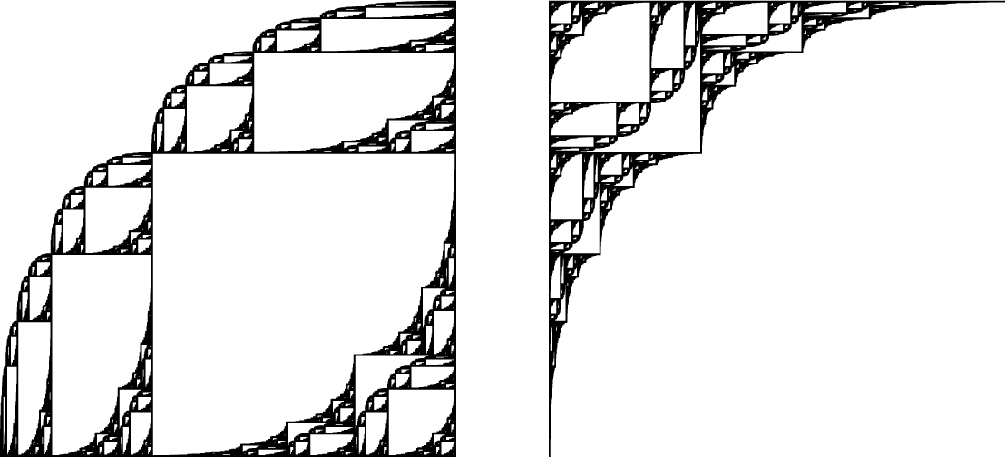
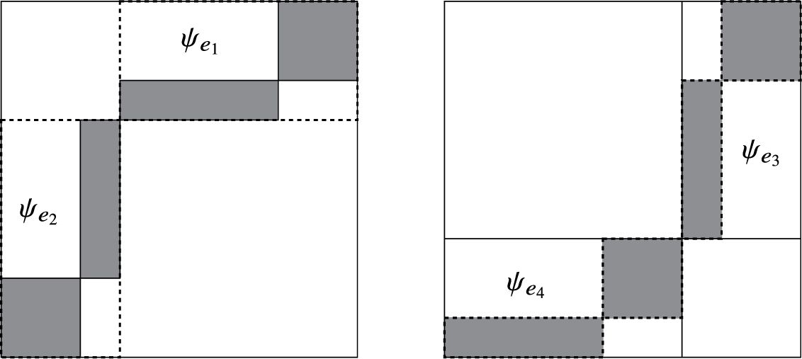
See Figure 1 for an example of associated graph-directed box-like self-affine set families. We will obtain a general exact closed form expression for
 $L^q$
-spectra of graph-directed self-affine measures, for general
 $q\geq 0$
. Specifically, returning to the diagonal IFS setting concerning Question 1.2, our result will state that the strict inequality (1.3) generally holds when (1.2) does not hold. Indeed, we will prove when
 $\min \{ \gamma _A(q),\gamma _B(q)\} \geq \tau _{\mu ^x}(q)+\tau _{\mu ^y}(q)$
,
 $$ \begin{align} \begin{aligned} \tau_\mu(q)&=\min \{x+y: \sum_{i=1}^N p_i^q a_i^x b_i^y=1, \tau_{\mu^x}(q)\leq x \leq \gamma_B(q)-\tau_{\mu^y}(q)\} \\&= \begin{cases} \gamma_A(q) &\text{ if}\ ({1.2\text{a}})\ \text{holds}, \\\gamma_B(q) &\text{ if}\ ({1.2\text{b}})\ \text{holds},\\<\min\{\gamma_A(q),\gamma_B(q)\} & \text{ otherwise. } \end{cases} \end{aligned} \end{align} $$
Not only that, we will illustrate that the above expression can alternatively be directly derived from Feng and Wang’s original result [Reference Feng and Wang19, Theorem 1] by using a careful Lagrange multipliers method. Another improvement of (1.4) is that it specifies the necessary and sufficient condition that
 $\tau _\mu (q)$
equals
 $\gamma _A(q)$
(respectively
 $\gamma _B(q)$
), compared with that in [Reference Fraser21].
An example of graph-directed box-like self-affine set families.

When allowing some maps to be anti-diagonal, our result is also a non-trivial extension of that of Morris’s [Reference Morris39] for box dimension (the
 $q=0$
case) to all
 $q\geq 0$
and to the GIFS setting. In his IFS setting, the graph-directed self-affine measure family degenerates to a single measure
 $\mu $
. The requirement that at least one of the
 $T_i$
in the IFS is anti-diagonal ensures that
 $\tau _{\mu ^x}(0)=\tau _{\mu ^y}(0)$
(taking
 $q=0$
) since
 $\{\mu ^x,\mu ^y\}$
becomes a strongly connected graph-directed self-similar measure family. However, in the GIFS setting, the graph-directed self-affine measure family
 $\{\mu _v\}_v$
will generate a collection of projection measures
 $\{\mu _v^x, \mu _v^y\}_v$
, which will be proved to be a disjoint union of one or two strongly connected self-similar measure families, and consequently, it may happen that
 $\tau _{\mu _v^x}(0)\neq \tau _{\mu _v^y}(0)$
. This will cause the main difficulty in the GIFS setting. Another main difficulty is to properly divide the consideration into distinct cases for distinct
 $q\geq 0$
.
An interesting observation of the closed form (1.4) is that it is possible to calculate the
 $L^q$
-spectrum of
 $\mu $
without involving the exact values of
 $\tau _{\mu ^x}(q)$
and
 $\tau _{\mu ^y}(q)$
. Indeed, for a large closed interval I, there always exist
 $x_0,y_0$
in I such that
 $$ \begin{align*} x_0+y_0= \min \bigg\{x+y: \sum_{i=1}^N p_i^q a_i^x b_i^y=1, x \in I\bigg\}. \end{align*} $$
Even if the exact values of
 $\tau _{\mu ^x}(q)$
and
 $\tau _{\mu ^y}(q)$
are unknown, if one can further find that
 $x_0\in [\tau _{\mu ^x}(q), \gamma _B(q)-\tau _{\mu ^y}(q)] \subset I$
, then
 $\tau _{\mu }(q)=x_0+y_0$
. In §3 (Example 3.4), we will present a collection of self-affine measures
 $\{\mu _{(a,b)}\}_{(a,b)\in \Gamma }$
for which this phenomenon occurs.
The motivation for extending the consideration to the GIFS setting is the potential application that we can use it to consider a box-like self-affine IFS of finite overlapping types, analogous to that of Ngai and Wang [Reference Ngai and Wang42] and the extension [Reference Lau and Ngai33] for self-similar IFS. We illustrate this in a recent paper [Reference Qiu, Wang and Wang47] concerning the
 $L^q$
-spectra for lower triangular planar non-conformal measures. We mention that there are also some previous works in the box-like self-affine GIFS setting. In [Reference Kenyon and Peres27], Kenyon and Peres extended the results of Bedford [Reference Bedford3] and McMullen [Reference McMullen36] computing the Hausdorff and box dimensions of graph-directed box-like self-affine sets with homogeneous grid structure. In [Reference Ni and Wen43], Ni and Wen considered the
 $L^q$
-spectra for graph-directed self-affine measures on Feng and Wang’s sets [Reference Feng and Wang19], in the setting that contraction ratios on the x-axis are always less than that on the y-axis for all maps in the GIFS, but additionally requiring contraction ratios on the x-axis to be arithmetic.
1.1 Basic setting and notation
The concept of a graph-directed iterated function system (GIFS) was first introduced by Mauldin and Williams [Reference Mauldin and Williams35].
Let
 $(V,E)$
be a finite directed graph with V being the vertex set and E being the directed edge set, allowing loops and multiple edges. For
 $e\in E$
, denote by
 $i(e)$
the initial vertex,
 $t(e)$
the terminal vertex of e, and sometimes write this as
 $i(e) \stackrel {e}{\rightarrow } t(e)$
. We always assume that for each
 $v\in V$
, there exists at least one edge
 $e\in E$
satisfying
 $i(e)=v$
.
Denote the collection of all finite admissible words by
 $$ \begin{align} E^*=\{w=w_1 \cdots w_k:t(w_{i-1})=i(w_{i}) \text{ for all } 1<i\leq k, k \in \mathbb{N}\}. \end{align} $$
For
 $w=w_1\cdots w_k\in E^*$
, denote
 $|w|=k$
the length of w,
 $i(w)=i(w_1)$
,
 $t(w)=t(w_k)$
the initial and terminal vertices of w, and also write
 $i(w) \stackrel {w}{\rightarrow } t(w)$
. For
 $w,w'\in E^*$
with
 $t(w)=i(w')$
, write
 $ww'$
the concatenation of w and
 $w'$
, and call w a prefix of
 $ww'$
. Denote
 $E^k$
the collection of all admissible words of length
 $k\geq 1$
.
For
 $v,v'\in V$
, we say that there exists a directed path from v to
 $v'$
if there exists
 $w\in E^*$
satisfying
 $v \stackrel {w}{\rightarrow }v'$
(write simply
 $v \to v'$
when we do not emphasize w). Write
 $v\nrightarrow v'$
if there is not a directed path from v to
 $v'$
. We say
 $(V,E)$
is strongly connected (or irreducible) if
 $v\to v'$
for all pairs
 $v,v'\in V$
.
For each
 $e\in E$
, we assume that there exists a contraction
 $\psi _e$
in the form of
 $\psi _e(\cdot )=T_e (\cdot ) +t_e$
, where
 $T_e$
is an
 $n\times n$
affine contracting matrix and
 $t_e \in \mathbb {R}^n$
. We write
 $\Psi =\{\psi _e\}_{e\in E}$
the collection of contraction
 $\psi _e$
. Call the triple
 $(V,E,\Psi )$
a self-affine GIFS. It is well known that there exists a unique family of compact sets
 $\{X_v\}_{v\in V}$
satisfying
 $$ \begin{align} X_v=\bigcup_{e\in E:i(e)=v} \psi_e(X_{t(e)})\quad \text{for all } v\in V. \end{align} $$
We call
 $\{X_v\}_{v\in V}$
a graph-directed self-affine set family associated with
 $(V,E,\Psi )$
. Note that if V is a singleton,
 $(V,E,\Psi )$
degenerates to a self-affine IFS and
 $\{X_v\}_{v\in V}$
degenerates to a self-affine set X.
Let
 ${\mathcal {P}}=(p_e)_{e\in E}$
be a positive vector satisfying
 $$ \begin{align} \sum_{e\in E:i(e)=v}p_e=1 \quad \text{for all } v\in V. \end{align} $$
It is known that there exists a unique finite family of probability measures
 $\{\mu _v\}_{v\in V} :=\{\mu _{{\mathcal {P}},v}\}_{v\in V}$
supported on
 $\{X_v\}_{v\in V}$
such that
 $$ \begin{align} \mu_v =\sum_{e\in E:i(e)=v} p_e \cdot \mu_{t(e)}\circ\psi_e^{-1} \quad \text{for all } v\in V. \end{align} $$
We call
 $\{\mu _v\}_{v\in V}$
a graph-directed self-affine measure family associated with
 ${\mathcal {P}}$
.
Throughout the paper, we assume that for each
 $e\in E$
,
 $T_e$
is a
 $2\times 2$
diagonal or anti-diagonal matrix of the form
 $$ \begin{align} T_e= \begin{pmatrix} \pm a_e & 0 \\ 0 & \pm b_e \\ \end{pmatrix} \quad \text{ or }\quad \begin{pmatrix} 0 & \pm a_e \\ \pm b_e & 0 \\ \end{pmatrix}, \end{align} $$
where
 $0<a_e,b_e <1$
. We call
 $(V,E,\Psi )$
a planar box-like self-affine GIFS,
 $\{X_v\}_{v\in V}$
a graph-directed box-like self-affine set family associated with
 $(V,E,\Psi )$
, and
 $\{\mu _v\}_{v\in V}$
a graph-directed box-like self-affine measure family. See Figures 2–4 for an example.
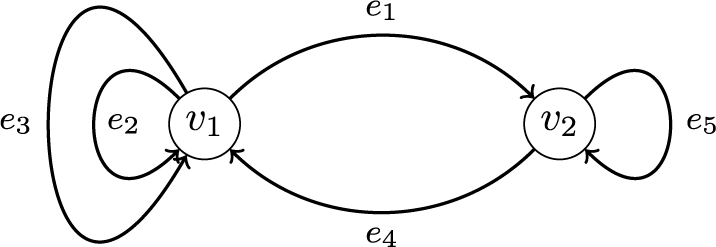
An example of directed graph
 $(V,E)$
.

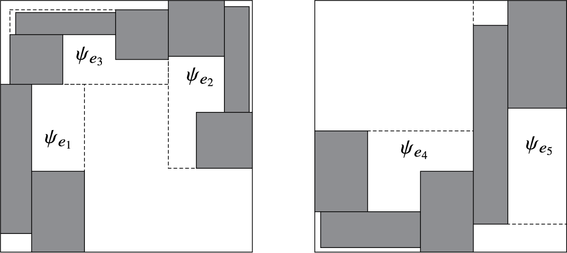
A planar box-like self-affine GIFS with
 $(V,E)$
illustrated in Figure 2, together with images of
 $[0,1]^2$
under the first and second level iterations of maps in this GIFS.

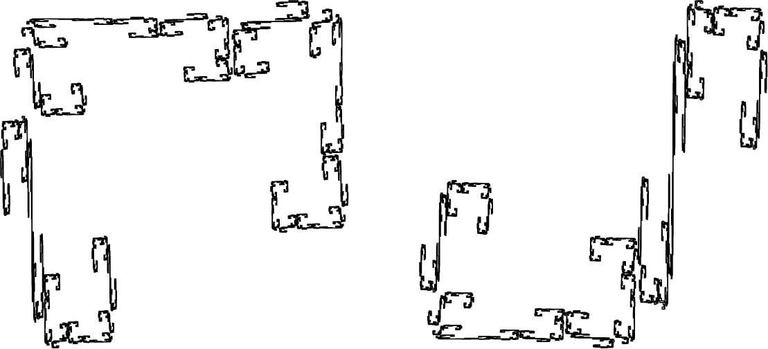
The graph-directed box-like self-affine set family
 $\{X_{v_1},X_{v_2}\}$
generated by the GIFS in Figure 3.

In this paper, we care about the
 $L^q$
-spectra of strongly connected planar graph-directed box-like self-affine measures
 $\{\mu _v\}_{v\in V}$
. For calculating the
 $L^q$
-spectra, we need the following separating condition for the planar box-like self-affine GIFS, which was first proposed by Feng and Wang [Reference Feng and Wang19] and plays crucial roles in subsequent works [Reference Falconer, Fraser and Lee11, Reference Fraser20, Reference Fraser21, Reference Fraser, Lee, Morris and Yu23].
Definition 1.3. (Rectangular open set condition)
We say a planar box-like self-affine GIFS
 $(V,E,\Psi )$
satisfies the rectangular open set condition (ROSC) if for all v in V,
 $$ \begin{align*} \bigcup_{e\in E:i(e)=v}\psi_e((0,1)^2)\subseteq(0,1)^2 \end{align*} $$
and the union is disjoint.
Our results rely on the
 $L^q$
-spectra of the projections of measures onto the x-axis or y-axis. Let
 $\pi _x$
,
 $\pi _y:\mathbb {R}^2\to \mathbb {R}$
be defined by
 $\pi _x(\xi _1,\xi _2)=\xi _1$
and
 $\pi _y(\xi _1,\xi _2)=\xi _2$
for
 $(\xi _1,\xi _2) \in \mathbb {R}^2$
, respectively. For each v in V, define
 $$ \begin{align} \mu_v^x=\mu_v\circ \pi_x^{-1}, \quad \mu_v^y=\mu_v\circ \pi_y^{-1} \end{align} $$
the projection measures of
 $\mu _v$
onto the x-axis and y-axis. Note that
 $\{\mu _v^x,\mu _v^y\}_{v\in V}$
is a family of graph-directed self-similar measures.
Proposition 1.4. [Reference Fraser21, Theorem 2.1]
For a strongly connected graph-directed self-similar measure family
 $\{\nu _v\}_{v\in V}$
, for all
 $q\geq 0$
and
 $v,v'\in V$
, we have
 $$ \begin{align*} \underline{\tau}_{\nu_v}(q)=\overline{\tau}_{\nu_v}(q) =\underline{\tau}_{\nu_{v'}}(q)=\overline{\tau}_{\nu_{v'}}(q), \end{align*} $$
that is, the
 $L^q$
-spectrum exists and is the same for every
 $\nu _v$
.
When
 $(V,E)$
is strongly connected and each
 $T_e$
is diagonal, both
 $\{\mu _v^x\}_{v\in V}$
and
 $\{\mu _v^y\}_{v\in V}$
are two strongly connected graph-directed self-similar measure families; when V is a singleton and
 $T_e$
is anti-diagonal for some
 $e\in E$
,
 $\{\mu _v^x, \mu _v^y\}$
is a strongly connected graph-directed self-similar measure family; for the general strongly connected case,
 $\{\mu _v^x, \mu _v^y\}_{v\in V}$
can be divided into one or two families of strongly connected graph-directed self-similar measures (see Proposition 2.1). By Proposition 1.4, we always have the
 $L^q$
-spectra exist for every
 $\mu _v^x$
,
 $\mu _v^y$
.
Throughout the paper, we will write
 $a\lesssim b$
for two variables (functions) if there is a constant
 $C>0$
such that
 $a\leq C\cdot b$
, and write
 $a\asymp b$
if both
 $a\lesssim b$
and
 $b\lesssim a$
hold. We write
 $a\lesssim _\theta b$
to mean that the constant depends on some parameter
 $\theta $
. Similarly, write
 $a \asymp _\theta b$
if both
 $a\lesssim _\theta b$
and
 $b\lesssim _\theta a$
hold. For two vectors
 $u=(u_i)$
and
 $v=(v_i)$
, we write
 $u\geq v$
if all
 $u_i\geq v_i$
. Also, for two matrices
 $A=(a_{ij})$
and
 $B=(b_{ij})$
, we write
 $A\geq B$
if all
 $a_{ij}\geq b_{ij}$
. For an
 $N\times N$
matrix A, for indices
 $\{i_1,\ldots ,i_k\}, \{j_1,\ldots , j_l\}$
with
 $k,l\leq N$
, we write
 $A[\{i_1,\ldots ,i_k\},\{j_1,\ldots , j_l\}]$
for a submatrix of A (lying in rows
 $\{i_1,\ldots ,i_k\}$
and columns
 $\{j_1,\ldots , j_l\}$
). We always write
 $\Vert \cdot \Vert $
for the
 $1$
-norm of a matrix, that is,
 $\Vert A \Vert =\sum _{i,j} |a_{ij}|$
. Let
 $\#A$
be the cardinality of a set A.
2 Results
In this section, we list the results in the paper, but postpone their proofs to later sections. Our main aim is to obtain the closed form expression for the
 $L^q$
-spectra of planar graph-directed box-like self-affine measures.
Throughout the following, we always let
 $(V,E,\Psi )$
be a strongly connected planar box-like self-affine GIFS,
 $\mathcal {P}$
be a positive vector satisfying (1.7), and
 $\{\mu _v\}_{v\in V}$
be a graph-directed box-like self-affine measure family satisfying (1.8) associated with
 $(V,E,\Psi )$
and
 $\mathcal {P}$
. Note that for each
 $e\in E$
, there exists a contraction
 $\psi _e$
in the form of
 $\psi _e(\cdot )=T_e(\cdot )+t_e$
for some
 $2\times 2$
diagonal or anti-diagonal contracting matrix
 $T_e$
satisfying (1.9) and
 $t_e\in \mathbb {R}^2$
. For
 $v\in V$
, we use
 $\mu _v^x$
(respectively
 $\mu _v^y$
) to denote the projection of
 $\mu _v$
onto the x-axis (respectively y-axis).
2.1 Existence of
$L^q$
-spectra

Before proceeding, we will prove in general that the
 $L^q$
-spectra of measures
 $\tau _{\mu _v^x}(q)$
,
 $\tau _{\mu _v^y}(q)$
, and
 $\tau _{\mu _v}(q)$
(under the ROSC) exist for all
 $q\geq 0$
and
 $v\in V$
, which will play fundamental roles in our later consideration. We will achieve this through the following Proposition 2.1 and Theorem 2.2 dealing with projection measures and original measures separately.
Proposition 2.1. Let
 $(V,E,\Psi )$
be a strongly connected planar box-like self-affine GIFS,
 $\mathcal P$
be an associated positive vector, and
 $\{\mu _v\}_{v\in V}$
be an associated graph-directed box-like self-affine measure family. Then,
 $$ \begin{align} \tau_{\mu_v^x}(q) \text{ and } \tau_{\mu_v^y}(q) \text{ exist } \quad \text{ for all } q\geq 0, v\in V. \end{align} $$
Moreover,
 $\{\mu _v^x,\mu _v^y\}_{v\in V}$
can be divided into two disjoint families A and B so that
 $$ \begin{align*}\#A=\#B=\#V,\end{align*} $$
such that for all
 $q\geq 0$
, there exist
 $\tau _A(q),\tau _B(q)$
satisfying
 $$ \begin{align} \begin{aligned} \tau_{\nu}(q)=\tau_A(q)\quad \text{ for all } \nu \in A,\\ \tau_{\nu}(q)=\tau_B(q)\quad \text{ for all } \nu \in B, \end{aligned} \end{align} $$
and that for all
 $v\in V$
,
 $$ \begin{align} \text{ either } \mu_v^x \in A, \mu_v^y\in B \quad \text{ or } \quad \mu_v^x \in B, \mu_v^y \in A. \end{align} $$
Note that when each
 $T_e$
is diagonal,
 $\{ \mu _v^x\}_{v\in V}$
and
 $\{ \mu _v^y\}_{v\in V}$
are two families of strongly connected graph-directed self-affine measures. By Proposition 1.4, without loss of generality, we could let
 $$ \begin{align*} A=\{ \mu_v^x\}_{v\in V} \quad \text{and}\quad B=\{ \mu_v^y\}_{v\in V}. \end{align*} $$
Due to Proposition 2.1, for
 $q\geq 0$
,
 $v\in V$
,
 $e\in E$
, throughout the paper, we will write
 $$ \begin{align} \begin{aligned} \tau_{x,v}(q)&:=\tau_{\mu_v^x}(q)\quad & & \text{and} & & \tau_{y,v}(q):=\tau_{\mu_v^y}(q),\\ \tau_{x,e}(q)&:=\tau_{x,t(e)}(q) & & \text{and} & &\tau_{y,e}(q):=\tau_{y,t(e)}(q) \end{aligned} \end{align} $$
for short. Also, write
 $$ \begin{align} t(q):=\tau_A(q)+\tau_B(q) \end{align} $$
for later use. Clearly, for all
 $v\in V$
,
 $\tau _{x,v}(q)+\tau _{y,v}(q)=t(q)$
.
Next, with Proposition 2.1 in hand, inspired by Fraser’s works [Reference Fraser20, Reference Fraser21] dealing with the box-like self-affine sets, that is, the case where
 $(V,E)$
degenerates to a singleton, we will introduce (in §4) a pressure function in the graph-directed setting,
 $$ \begin{align*}P:\mathbb{R}\times[0,\infty) \to \mathbb{R},\end{align*} $$
based on certain modified singular value function matrices. For each
 $q\geq 0$
, as a function of s,
 $P(s,q)$
will be strictly decreasing and continuous, tending to
 $0$
as
 $s \to +\infty $
and to
 $+\infty $
as
 $s\to -\infty $
. Using this, we will define a function
 $\gamma :[0,\infty )\to \mathbb {R}$
by setting
 $$ \begin{align*}P(\gamma(q),q)=1.\end{align*} $$
Theorem 2.2. Let
 $(V,E,\Psi )$
be a strongly connected planar box-like self-affine GIFS,
 $\mathcal P$
be an associated positive vector, and
 $\{\mu _v\}_{v\in V}$
be an associated graph-directed box-like self-affine measure family. Then, we obtain the following.
-
(a) For all
$q\in [0,1],$
we have
$$ \begin{align*} \overline{\tau}_{\mu_v}(q)\leq \gamma(q) \quad \text{ for all }v\in V. \end{align*} $$
-
(b) For all
$q\in [1,+\infty )$
, we have
$$ \begin{align*} \underline{\tau}_{\mu_v}(q)\geq \gamma(q) \quad \text{ for all }v\in V. \end{align*} $$
-
(c) If
$(V,E,\Psi )$
satisfies the ROSC, then for all
$q\geq 0$
,
$$ \begin{align*} \tau_{\mu_v}(q)= \gamma(q) \quad \text{ for all }v\in V. \end{align*} $$


Proposition 2.1 will be proved in §4. The details for pressure function P will be presented also in §4. The proof of Theorem 2.2 will be postponed to §5.
2.2 Closed form expression in GIFS setting
From definition, for
 $q\geq 0$
,
 $\gamma (q)$
does not seem to be able to be explicitly computed through a finite amount of steps. So, our next aim is to find a closed form expression for
 $\gamma (q)$
.
2.2.1 General setting
For
 $q\geq 0$
,
 $x,y\in \mathbb {R}$
,
 $e,e'\in E$
, define a
 $2\times 2$
matrix with indices
 $\{e(1),e(2)\}\times \{e'(1),e'(2)\}$
,
 $$ \begin{align*} G^{(q)}_{x,y,e,e'} = \begin{cases} \!\!\!\!\! &\begin{aligned} \begin{pmatrix} p_{e'}^q a_{e'}^{x+\tau_{x,e'}(q)} b_{e'}^{y-\tau_{x,e'}(q)} & 0 \\ 0 & p_{e'}^q b_{e'}^{x+\tau_{y,e'}(q)} a_{e'}^{y-\tau_{y,e'}(q)} \\ \end{pmatrix}\hspace{2.45cm} \\ \text{ if } t(e)=i(e') \text{ and }T_{e'} \text{ is diagonal, } \end{aligned}\\ \!\!\!\!\!&\begin{aligned} \begin{pmatrix} 0 & p_{e'}^q a_{e'}^{x+\tau_{y,e'}(q)} b_{e'}^{y-\tau_{y,e'}(q)} \\ p_{e'}^q b_{e'}^{x+\tau_{x,e'}(q)} a_{e'}^{y-\tau_{x,e'}(q)} &0 \\ \end{pmatrix} \hspace{3cm} \\ \text{ if } t(e)=i(e') \text{ and } T_{e'} \text{ is anti-diagonal,} \end{aligned}\\ \!\!\!\!\!&\begin{aligned} \begin{pmatrix} 0 & 0 \\ 0 &0 \\ \end{pmatrix} \hspace{3.65cm} \text{otherwise. } \end{aligned} \end{cases} \end{align*} $$
Define a
 $\# E \times \# E$
block function matrix
 $\mathcal {G}_{x,y}^{(q)}$
with entries being
 $2\times 2$
matrices,
 $$ \begin{align} \mathcal{G}_{x,y}^{(q)}[\{e(1),e(2)\},\{e'(1),e'(2)\}] = G_{x,y,e,e'}^{(q)}, \end{align} $$
and regard
 $\mathcal {G}_{x,y}^{(q)}$
as a
 $(2\#E)\times (2\#E)$
matrix. Define a function
 $\hat {\gamma }(q):[0,+\infty ) \to \mathbb {R}$
so that for each q,
 $\hat {\gamma }(q)$
is the unique solution of
 $$ \begin{align} \rho(\mathcal{G}^{(q)}_{0,\hat{\gamma}(q)})=\rho(\mathcal{G}^{(q)}_{\hat{\gamma}(q)-t(q),t(q)})=1 \end{align} $$
(to be well defined in Remark 6.7), where
 $\rho (\cdot )$
is the spectral radius of a matrix. The following theorem is our main result.
Theorem 2.3. Let
 $(V,E,\Psi ),\mathcal {P}, \{\mu _v\}_{v\in V}$
and
 $\gamma $
be the same as in Theorem 2.2. For
 $q\geq 0$
, we have the following.
-
(a) If
$\hat {\gamma }(q)\leq t(q)$
, (2.8)
$$ \begin{align} \gamma(q)&=\hat{\gamma}(q) \notag\\ &= \max \{x+y: \rho(\mathcal{G}^{(q)}_{x,y})=1, \hat{\gamma}(q)-t(q) \leq x \leq 0 \}\notag\\ &=\max \{x+y: \rho(\mathcal{G}^{(q)}_{x,y})=1, \hat{\gamma}(q) \leq y \leq t(q) \}. \end{align} $$
-
(b) If
$\hat {\gamma }(q)>t(q)$
, (2.9)
$$ \begin{align} \gamma(q)&=\min \{x+y: \rho(\mathcal{G}^{(q)}_{x,y})=1, 0 \leq x \leq \hat{\gamma}(q)-t(q) \}\notag\\ &=\min \{x+y: \rho(\mathcal{G}^{(q)}_{x,y})=1, t(q)\leq y \leq \hat{\gamma}(q)\}. \end{align} $$


2.2.2 Diagonal setting
Suppose each
 $T_e$
is of the form
 $$ \begin{align*} T_e= \begin{pmatrix} \pm a_e & 0 \\ 0 & \pm b_e \\ \end{pmatrix}. \end{align*} $$
In this setting, recall
 $A=\{\mu _v^x\}_{x\in V}$
,
 $B=\{\mu _v^y\}_{v\in V}.$
By Proposition 2.1, for all
 $v\in V$
,
 $\tau _{x,v}(q)=\tau _A(q)$
,
 $\tau _{y,v}(q)=\tau _B(q)$
, and
 $\tau _{x,v}(q)+\tau _{y,v}(q)=t(q).$
For
 $q\geq 0$
,
 $x,y\in \mathbb {R}$
, we introduce (in §6.3) a
 $\#E \times \#E$
function matrix
 $F^{(q)}_{x,y}$
with entries defined by
 $$ \begin{align} F^{(q)}_{x,y}(e,e') =\begin{cases} p_{e'}^q a_{e'}^x b_{e'}^y & \text{ if } t(e)=i(e'),\\ 0 & \text{ otherwise}. \end{cases} \end{align} $$
Then, define two functions
 $\gamma _A,\gamma _B:[0,+\infty)\to \mathbb {R}$
such that for
 $q\geq 0$
,
 $\gamma _A(q)$
and
 $\gamma _B(q)$
are the unique solutions of
 $$ \begin{align} \rho(F^{(q)}_{\tau_A(q),\gamma_A(q)-\tau_A(q)})=1 \end{align} $$
and
 $$ \begin{align} \rho(F^{(q)}_{\gamma_B(q)-\tau_B(q),\tau_B(q)})=1, \end{align} $$
respectively (to be well defined in §6.3).
Corollary 2.4. Let
 $(V,E,\Psi )$
,
 ${\mathcal {P}}$
,
 $\{\mu _v\}_{v \in V}$
and
 $\gamma $
be the same as in Theorem 2.3. Assume that every
 $T_e$
is diagonal. Then, for
 $q\geq 0 $
,
 $$ \begin{align} \text{ either } \max \{\gamma_A(q), \gamma_B(q)\} \leq t(q) \end{align} $$
 $$ \begin{align} \text{ or } \min \{\gamma_A(q), \gamma_B(q)\} \geq t(q). \end{align} $$
-
(a) If (2.13a) holds,
(2.14)
$$ \begin{align} \gamma(q)&=\max \{\gamma_A(q), \gamma_B(q)\} \notag\\ &= \max \{x+y: \rho(F^{(q)}_{x,y})=1, \gamma_B(q)-\tau_B(q) \leq x \leq \tau_A(q) \} \notag\\ &=\max \{x+y: \rho(F^{(q)}_{x,y})=1, \gamma_A(q)-\tau_A(q) \leq y \leq \tau_B(q) \}. \end{align} $$
-
(b) If (2.13b) holds,
(2.15)
$$ \begin{align} \gamma(q)&=\min \{x+y: \rho(F^{(q)}_{x,y})=1, \tau_A(q)\leq x \leq \gamma_B(q)-\tau_B(q) \} \notag\\ &=\min \{x+y: \rho(F^{(q)}_{x,y})=1, \tau_B(q)\leq y \leq \gamma_A(q)-\tau_A(q) \}. \end{align} $$


Remark 2.5. Return to the diagonal IFS setting, for case (b), we can further see that
 $\gamma (q)<\min \{\gamma _A(q),\gamma _B(q)\}$
may occur, see Corollary 2.9.
2.2.3 The
$q=0$
case

Recall that when
 $q=0$
, the
 $L^q$
-spectrum of a measure
 $\nu $
is equal to the box dimension of
 $\text {supp} \nu $
.
Corollary 2.6. Let
 $(V,E,\Psi )$
be the same as in Theorem 2.3. Let
 $\{X_v\}_{v\in V}$
be the unique graph-directed box-like self-affine set family associated with
 $(V,E,\Psi )$
. Assume that
 $(V,E,\Psi )$
satisfies the ROSC. Then, for all
 $v\in V$
,
 $$ \begin{align*} \dim_B X_v =\hat{\gamma}(0). \end{align*} $$
In particular, if each
 $T_e$
is diagonal, for all
 $v\in V$
,
 $$ \begin{align*} \dim_B X_v=\max \{\gamma_A(0), \gamma_B(0)\}. \end{align*} $$
2.3 Closed form expression in IFS setting
When V is a singleton,
 $(V,E,\Psi )$
degenerates to a box-like self-affine IFS,
 $\mathcal P$
degenerates to a positive probability vector, and
 $\{\mu _v\}_{v\in V}$
degenerates to a single measure
 $\mu $
. The directed edge set E can be written as
 $\{1,\ldots , N\}$
. Without loss of generality, by rearranging the order of
 $\{\psi _i\}_{i=1}^N$
, we can assume that there is a
 $k\in \{1,\ldots ,N+1\}$
so that
 $$ \begin{align*} T_i=\begin{cases} \begin{pmatrix} \pm a_i & 0 \\ 0 & \pm b_i \\ \end{pmatrix} & \text{ if } 1\leq i< k,\\[9pt] \begin{pmatrix} 0 & \pm a_i \\ \pm b_i & 0 \\ \end{pmatrix} & \text{ if } k\leq i\leq N. \end{cases} \end{align*} $$
Note that when
 $k=N+1$
, each
 $T_i$
is diagonal.
For
 $q\geq 0, x,y\in \mathbb {R}$
, define a
 $2 \times 2 $
function matrix
 $$ \begin{align} H^{(q)}_{x,y}=\begin{pmatrix} \displaystyle\sum_{i=1}^{k-1} p_i^q a_i^{x+\tau_{\mu^x}(q)} b_i^{y-\tau_{\mu^x}(q)} & \displaystyle\sum_{i=k}^N p_i^q a_i^{x+\tau_{\mu^y}(q)} b_i^{y-\tau_{\mu^y}(q)}\\[10pt] \displaystyle\sum_{i=k}^N p_i^q b_i^{x+\tau_{\mu^x}(q)} a_i^{y-\tau_{\mu^x}(q)} & \displaystyle\sum_{i=1}^{k-1} p_i^q b_i^{x+\tau_{\mu^y}(q)} a_i^{y-\tau_{\mu^y}(q)}\end{pmatrix}. \end{align} $$
Corollary 2.7. Let
 $\{\psi _i(\cdot ) =T_i (\cdot )+t_i\}_{i=1}^N$
be a box-like self-affine IFS satisfying the ROSC. Let
 $\mathcal {P}=(p_i)_{i=1}^N$
be a positive probability vector. Let
 $\mu $
be the self-affine measure associated with
 $\mathcal {P}$
. For
 $q\geq 0$
,
 $\hat {\gamma }(q)$
satisfies
 $$ \begin{align} \rho(H^{(q)}_{0,\hat{\gamma}(q)})=\rho(H^{(q)}_{\hat{\gamma}(q)-t(q),t(q)})=1. \end{align} $$
In addition, we have the following.
-
(a) If
$\hat {\gamma }(q)\leq t(q)$
,
$$ \begin{align*} \begin{aligned} \tau_{\mu}(q)&=\hat{\gamma}(q)\\ &= \max \{x+y: \rho(H^{(q)}_{x,y})=1, \hat{\gamma}(q)-t(q)\leq x \leq 0 \}\\ &=\max \{x+y: \rho(H^{(q)}_{x,y})=1, \hat{\gamma}(q) \leq y \leq t(q) \}. \end{aligned} \end{align*} $$
-
(b) If
$\hat {\gamma }(q)>t(q)$
,
$$ \begin{align*} \begin{aligned} \tau_{\mu}(q)&=\min \{x+y: \rho(H^{(q)}_{x,y})=1, 0\leq x \leq \hat{\gamma}(q)-t(q) \}\\ &=\min \{x+y: \rho(H^{(q)}_{x,y})=1, t(q)\leq y \leq \hat{\gamma}(q)\}. \end{aligned} \end{align*} $$


Remark 2.8. Morris’ closed form expression [Reference Morris39, Proposition 5] for box dimensions of box-like self-affine sets can be seen by combining Corollaries 2.6 and 2.7 together and taking
 $q=0$
.
Now, we return to the diagonal self-affine IFS setting. At this time, all rows of the matrix
 $F^{(q)}_{x,y}$
are the same. So by the Perron–Frobenius theorem,
 $\rho (F^{(q)}_{x,y})= \sum _{i=1}^N p_i^q a_i ^x b_i^y$
. Thus,
 $\gamma _A,\gamma _B$
can be reduced to the unique solutions satisfying
 $$ \begin{align*} \sum_{i=1}^N p_i^q a_i^{\tau_A(q)} b_i^{\gamma_A(q)-\tau_A(q)}=1 \end{align*} $$
and
 $$ \begin{align*} \sum_{i=1}^N p_i^q a_i^{\gamma_B(q)-\tau_B(q)} b_i^{\tau_B(q)}=1, \end{align*} $$
respectively. Recall the following two conditions in (1.2):
 $$ \begin{align} \sum_{i=1}^N p_i^q a_i^{\tau_A(q)} b_i^{\gamma_A(q)-\tau_A(q)} \log a_i/b_i\geq 0 \end{align} $$
and
 $$ \begin{align} \sum_{i=1}^N p_i^q b_i^{\tau_B(q)} a_i^{\gamma_B(q)-\tau_B(q)} \log a_i/b_i\leq 0. \end{align} $$
We obtain the following corollary, a precise answer to [Reference Fraser21, Question 2.14].
Corollary 2.9. Let
 $\{\psi _i(\cdot ) =T_i (\cdot )+t_i\}_{i=1}^N$
be a box-like self-affine IFS satisfying the ROSC. Assume that every
 $T_i$
is diagonal. Let
 $\mathcal {P}=(p_i)_{i=1}^N$
be a positive probability vector. Let
 $\mu $
be the self-affine measure associated with
 $\mathcal {P}$
. For
 $q\geq 0$
,
 $$ \begin{align} \text{ either } &\max \{\gamma_A(q), \gamma_B(q)\} \leq t(q) \end{align} $$
 $$ \begin{align} \text{ or } &\min \{\gamma_A(q), \gamma_B(q)\} \geq t(q). \end{align} $$
-
(a) If (2.19a) holds,
$$ \begin{align*} \begin{aligned} \tau_{\mu}(q)&=\max \{\gamma_A(q), \gamma_B(q)\}\\ &= \max \bigg\{x+y: \sum_{i=1}^N p_i^q a_i^x b_i^y=1, \gamma_B(q)-\tau_B(q) \leq x \leq \tau_A(q) \bigg\}\\ &= \max \bigg\{x+y: \sum_{i=1}^N p_i^q a_i^x b_i^y=1, \gamma_A(q)-\tau_A(q) \leq y \leq \tau_B(q) \bigg\}. \end{aligned} \end{align*} $$
-
(b) If (2.19b) holds,
Moreover, we have the following.
$$ \begin{align*} \begin{aligned} \tau_{\mu}(q)&=\min \bigg\{x+y: \sum_{i=1}^N p_i^q a_i^x b_i^y=1, \tau_A(q)\leq x \leq \gamma_B(q)-\tau_B(q) \bigg\}\\ &=\min \bigg\{x+y: \sum_{i=1}^N p_i^q a_i^x b_i^y=1, \tau_B(q)\leq y \leq \gamma_A(q)-\tau_A(q) \bigg\}. \end{aligned} \end{align*} $$
-
(b1) If (2.18a) holds,
$\tau _{\mu }(q)=\gamma _A(q).$
-
(b2) If (2.18b) holds,
$\tau _{\mu }(q)=\gamma _B(q).$
-
(b3) Otherwise, there exist
$x\in [\tau _A(q),\gamma _B(q)-\tau _B(q)]$
and
$y \in [\tau _B(q),\gamma _A(q)-\tau _A(q)]$
satisfying
$\sum _{i=1}^N p_i^q a_i^x b_i^y=1$
such that
$\sum _{i=1}^N p_i^q a_i^x b_i^y\log (a_i/b_i) =0$
and
$$ \begin{align*} \tau_{\mu}(q)=x+y < \min \{\gamma_A(q),\gamma_B(q)\}. \end{align*} $$
-


Remarks 2.10.
-
(a) Fraser [Reference Fraser21, Theorem 2.10] proved that if (2.19b) holds,
$\tau _{\mu }(q)\leq \min \{ \gamma _A(q),\gamma _B(q)\}$
with equality if either (2.18a) or (2.18b) holds. Indeed, he proved that
$\tau _{\mu }(q)=\gamma _A(q)$
if (2.18a) holds, and
$\tau _{\mu }(q)=\gamma _B(q)$
if (2.18b) holds. -
(b) Corollary 2.9 can also be directly derived by using [Reference Feng and Wang19, Theorem 1] without using Corollary 2.4, see §6.5.


We will consider the closed form expression in §6, where we will prove Theorem 2.3 and Corollaries 2.4, 2.6, 2.7, and 2.9. Particularly, we will provide an alternative proof of Corollary 2.9 in §6.5.
3 Examples
In this section, we provide three examples to illustrate our results. The first two are in the self-affine IFS setting and the third is in the self-affine GIFS setting.
Example 3.1. For some
 $a,b\in (0,1)$
with
 $a+b\leq 1$
, let
 $$ \begin{align*} \psi_1\begin{pmatrix} \xi_1 \\ \xi_2 \end{pmatrix} = \begin{pmatrix} &a &0\\ &0 &b \end{pmatrix} \begin{pmatrix} &\xi_1\\ &\xi_2 \end{pmatrix}\quad \text{and} \quad \psi_2\begin{pmatrix} \xi_1 \\ \xi_2 \end{pmatrix} = \begin{pmatrix} &b &0\\ &0 &a \end{pmatrix} \begin{pmatrix} &\xi_1\\ &\xi_2 \end{pmatrix} + \begin{pmatrix} &1-b\\ &1-a \end{pmatrix}. \end{align*} $$
Then,
 $\{\psi _1, \psi _2\}$
becomes a planar box-like self-affine IFS. Let X be its attractor. Let
 $$ \begin{align*} \psi^{\prime}_1\begin{pmatrix} \xi_1 \\ \xi_2 \end{pmatrix} = \begin{pmatrix} 0 &a\\ b &0 \end{pmatrix} \begin{pmatrix} \xi_1\\ \xi_2 \end{pmatrix}\quad \text{and} \quad \psi^{\prime}_2=\psi_2, \end{align*} $$
and
 $X'$
be the attractor of the planar box-like self-affine IFS
 $\{\psi _1',\psi _2'\}$
. Note that the images of
 $\psi _1$
and
 $\psi _1'$
(respectively
 $\psi _2$
and
 $\psi _2'$
) under
 $[0,1]^2$
are the same. See Figure 5 for
 $X,X'$
when
 $a=3/4,b=1/4$
.
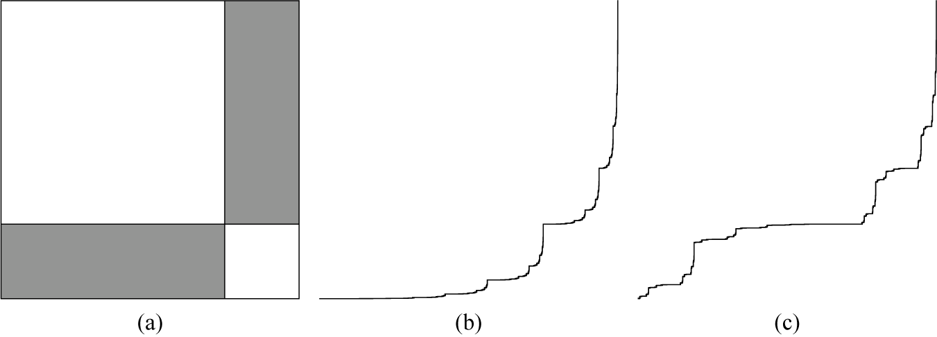
(a) The shaded rectangles are images of the iterated function
 $\psi _1$
(respectively
 $\psi _1'$
) and
 $\psi _2$
(respectively
 $\psi _2'$
). (b) The attractor X. (c) The attractor
 $X'$
.

Let
 $\mu $
(respectively
 $\mu '$
) be the self-affine measure associated with
 $\{\psi _1,\psi _2\}$
(respectively
 $\{\psi _1',\psi _2'\}$
) and a probability vector
 $\mathcal {P}=(1/2,1/2)$
.
Proposition 3.2. For the measures
 $\mu $
,
 $\mu '$
in Example 3.1, we have
 $$ \begin{align} \tau_{\mu}(q)=\tau_{\mu'}(q)= \begin{cases} s(q) & \text{if } q\in[0,1],\\ \dfrac{2(q-1)\log 2}{\log ab} &\text{if } q\in [1,\infty), \end{cases} \end{align} $$
where
 $s(q)$
is the unique solution of
 $(\tfrac 12)^q a^{s(q)} + (\tfrac 12)^q b^{s(q)}=1.$
Remark 3.3. The box-like self-affine IFS
 $\{\psi _1,\psi _2\}$
was considered in [Reference Fraser, Lee, Morris and Yu23], which illustrated that
 $ \tau _{\mu }(q) <\min \{\gamma _A(q),\gamma _B(q)\} $
may happen. We point out that in [Reference Kolossváry30, Proposition 4.4], Kolossváry obtained an exact expression of
 $\tau _\mu (q)$
for general self-affine measures and for all
 $q\in \mathbb {R}$
. Particularly, for the
 $L^q$
-dimension defined as
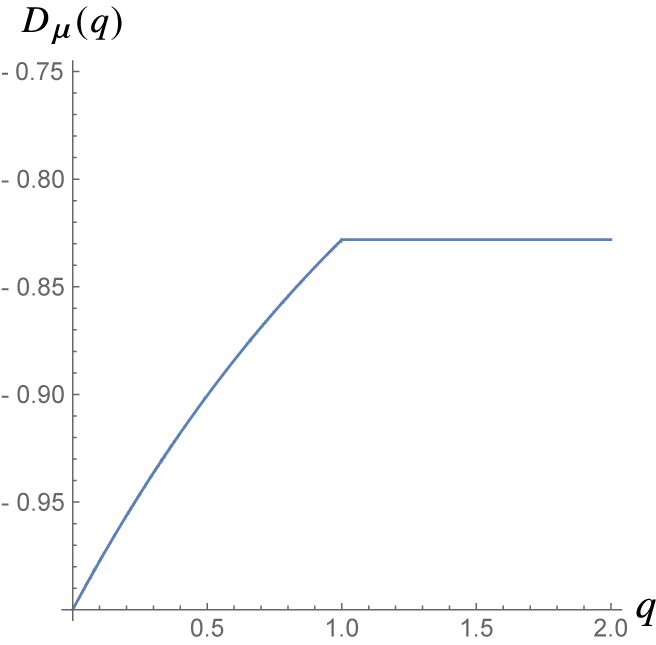
 $D_\mu (q):= ({\tau _\mu (q)})/({q-1})$
, an interesting phase transition phenomenon was revealed (see Figure 6), which answered [Reference Fraser, Lee, Morris and Yu23, Question 3.10].
The graph of
 $L^q$
-dimension of
 $\mu $
by setting
 $a=3/4$
,
 $b=1/4$
.

Proof of Proposition 3.2 for
$\mu $

For
 $q\geq 0$
, it is easy to check that
 $\tau _{\mu ^x}(q)=\tau _{\mu ^y}(q)$
and equals
 $s(q)$
. So,
 $\gamma _A(q)=\gamma _B(q)$
and equals the unique solution
 $r(q)$
of
 $$ \begin{align} (\tfrac{1}{2} )^q a^{s(q)} b^{r(q)-s(q)} + (\tfrac{1}{2} )^q b^{s(q)} a^{r(q)-s(q)} =1. \end{align} $$
Combining this with the definition of
 $s(q)$
, we see that
 $r(q)=s(q)$
. We can use either Corollary 2.9 or Corollary 2.7 to calculate the closed form expression for
 $\tau _{\mu }(q)$
,
 $q\geq 0.$
Using Corollary 2.9. Note that
 $\max \{\gamma _A(q),\gamma _B(q)\} \leq \tau _{\mu ^x}(q)+\tau _{\mu ^y}(q)$
is equivalent to
 $s(q)\geq 0$
, which is further equivalent to
 $q\leq 1$
. By Corollary 2.9, we know that
 $$ \begin{align} \tau_{\mu}(q)= \begin{cases} s(q) &\text{ if } q\in[0,1], \\ \min \{x+y:( \tfrac{1}{2})^q a^{x} b^{y} + ( \tfrac{1}{2} )^q b^{x} a^{y} =1, s(q)\leq x \leq 0\} & \text{ if } q\in [1,\infty). \end{cases} \end{align} $$
Consider the implicit function
 $y(x)$
determined by
 $( \tfrac 12 )^q a^{x} b^{y(x)} + ( \tfrac 12 )^q b^{x} a^{y(x)} =1$
. Take
 $x={{(q-1)\log 2}}/{(\log ab)}$
, so that
 $y'(x)=-1$
and
 $$ \begin{align} 2x=x+y(x)=\min \{ x+y:( \tfrac{1}{2} )^q a^{x} b^{y} + ( \tfrac{1}{2} )^q b^{x} a^{y} =1\}. \end{align} $$
When
 $q\in [1,\infty )$
, noticing that
 $s(q)\leq 0$
, we get
 $$ \begin{align*} 2(\tfrac{1}{2})^q (ab)^{x}=1=(\tfrac{1}{2})^q a^{s(q)} + (\tfrac{1}{2})^q b^{s(q)}\leq 2(\tfrac{1}{2})^q (ab)^{s(q)}, \end{align*} $$
which gives that
 $x\geq s(q)$
. Clearly, also we have
 $x\leq 0$
. Combining this with (3.3) and (3.4), we can arrive at (3.1).
Using Corollary 2.7. Let
 $H^{(q)}_{x,y}$
be the following matrix:
 $$ \begin{align*} \begin{pmatrix} (\tfrac{1}{2})^q a^{x+s(q)} b^{y-s(q)}+ (\tfrac{1}{2})^q b^{x+s(q)}a^{y-s(q)} \!\! & 0\\ 0 & \!\! (\tfrac{1}{2})^q b^{x+s(q)} a^{y-s(q)}+(\tfrac{1}{2})^q a^{x+s(q)} b^{y-s(q)}\\ \end{pmatrix}\!. \end{align*} $$
Then,
 $$ \begin{align*} \rho(H^{(q)}_{x,y})=(\tfrac{1}{2})^q a^{x+s(q)} b^{y-s(q)}+(\tfrac{1}{2})^q b^{x+s(q)}a^{y-s(q)}. \end{align*} $$
Thus, by taking
 $x=0$
in the above equation,
 $\hat {\gamma }(q)=r(q)$
by using (3.2). Note that when
 $q\in [1,\infty )$
,
 $$ \begin{align*} &\min \{x+y: (\tfrac{1}{2})^q a^{x+s(q)} b^{y-s(q)}+(\tfrac{1}{2})^q b^{x+s(q)}a^{y-s(q)}=1,0\leq x \leq -s(q)\}\\ & \quad = \min \{ x+y:( \tfrac{1}{2})^q a^{x} b^{y} + (\tfrac{1}{2})^q b^{x} a^{y} =1,s(q)\leq x \leq 0\}. \end{align*} $$
Therefore, we still get (3.3) and so (3.1) also follows by Corollary 2.7.
Proof of Proposition 3.2 for
$\mu '$

Noticing that the linear part of
 $\psi _1'$
is anti-diagonal,
 $\{\mu ^{\prime {x}},\mu ^{\prime {y}}\}$
is a strongly connected self-similar graph-directed measure family, that is,
 $$ \begin{align*} \mu^{\prime{x}}(I)=\tfrac{1}{2} \mu^{\prime{y}}(aI)+\tfrac{1}{2} \mu^{\prime{x}}(bI+1-b) \end{align*} $$
and
 $$ \begin{align*} \mu^{\prime{y}}(I)=\tfrac{1}{2} \mu^{\prime{x}}(bI)+\tfrac{1}{2} \mu^{\prime{y}}(aI+1-a) \end{align*} $$
for all Borel sets
 $I \subseteq \mathbb {R}.$
Let
 $\beta (q)$
be the unique solution of
 $$ \begin{align*} \rho \begin{pmatrix} (\tfrac{1}{2})^q b^{\beta(q)} & (\tfrac{1}{2})^q a^{\beta(q)} \\ (\tfrac{1}{2})^q b^{\beta(q)} & (\tfrac{1}{2})^q a^{\beta(q)} \end{pmatrix} = (\tfrac{1}{2})^q b^{\beta(q)} + (\tfrac{1}{2})^q a^{\beta(q)} =1. \end{align*} $$
It follows from the result in [Reference Strichartz51] that
 $\tau _{\mu ^{\prime {x}}}(q)=\tau _{\mu ^{\prime {y}}}(q)=\beta (q).$
So,
 $\tau _{\mu ^{\prime {x}}}(q)=\tau _{\mu ^{\prime {y}}}(q)=\tau _{\mu ^x}(q)=\tau _{\mu ^y}(q)$
and
 $\beta (q)=s(q)$
by the definition of
 $s(q)$
. Take
 $$ \begin{align*} H^{\prime(q)}_{x,y}= \begin{pmatrix} (\tfrac{1}{2})^q b^{x+\beta(q)}a^{y-\beta(q)} & (\tfrac{1}{2})^q a^{x+\beta(q)} b^{y-\beta(q)}\\ (\tfrac{1}{2})^q b^{x+\beta(q)} a^{y-\beta(q)} & (\tfrac{1}{2})^q a^{x+\beta(q)} b^{y-\beta(q)} \end{pmatrix}, \end{align*} $$
which implies that
 $$ \begin{align*} \rho(H^{\prime(q)}_{x,y})=(\tfrac{1}{2})^q b^{x+\beta(q)}a^{y-\beta(q)} + (\tfrac{1}{2})^q a^{x+\beta(q)} b^{y-\beta(q)}=\rho(H^{(q)}_{x,y}). \end{align*} $$
So,
 $\tau _{\mu '}(q)=\tau _{\mu }(q)$
for
 $q\geq 0$
by Corollary 2.7. Thus, (3.1) holds for
 $\mu '$
.
Example 3.4. Define
 $\Gamma\hspace{-1pt} =\hspace{-1pt}\{(a,b)\hspace{-1pt}\in\hspace{-1pt} (0,1)^2: a\hspace{-1pt}+\hspace{-1pt}b\leq 1, ({\log b}/{\log a})\leq \tfrac 13\}$
. For
 $(a,b)\hspace{-1pt}\in\hspace{-1pt} \Gamma $
, define an IFS
 $$ \begin{align*} \Psi_{(a,b)} =\bigg\{ \begin{pmatrix} a & 0 \\ 0 & a \end{pmatrix} \begin{pmatrix} \xi_1 \\ \xi_2 \end{pmatrix}, \begin{pmatrix} b &0\\ 0 &a \end{pmatrix} \begin{pmatrix} \xi_1\\ \xi_2 \end{pmatrix}+ \begin{pmatrix} 0\\ 1-a \end{pmatrix}, \begin{pmatrix} a & 0 \\ 0 & b \end{pmatrix} \begin{pmatrix} \xi_1 \\ \xi_2 \end{pmatrix} + \begin{pmatrix} 1-a\\ 0 \end{pmatrix} \bigg\}. \end{align*} $$
For each
 $(a,b)\in \Gamma $
, let
 $X_{(a,b)}$
be the self-affine set generated by
 $\Psi _{(a,b)}$
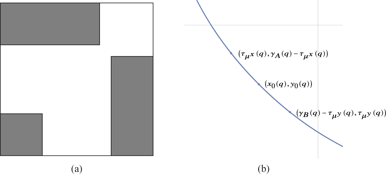
, see Figure 7(a).
(a) The shaded rectangles are images of the IFS
 $\Psi _{(a,b)}$
. (b) The graph of the curve
 $\{(x,y): (\tfrac 13)^q(a^{x+y}+a^xb^y+b^xa^y)=1\}$
.

Let
 $\mu _{(a,b)}$
be a self-affine measure on
 $X_{(a,b)}$
associated with a probability vector
 $(1/3,1/3,1/3)$
. At this time,
 $\mu _{(a,b)}^x= \mu _{(a,b)}^y$
are self-similar measures. Although we are unclear about the information of
 $\tau _{\mu _{(a,b)}^x}(q)$
and
 $\tau _{\mu _{(a,b)}^y}(q)$
(note that (1.1) does not hold as the exact overlap occurs), we still can derive the exact values of
 $\tau _{\mu _{(a,b)}}(q)$
providing
 $(a,b)\in \Gamma $
and q sufficiently large.
Proposition 3.5. There is a sufficiently large
 $q_0\geq 1$
, such that for each
 $(a,b)\in \Gamma $
,
 $q\geq q_0$
, we have
 $$ \begin{align*} \tau_{\mu_{(a,b)}}(q)=2x_0(q), \end{align*} $$
where
 $x_0(q)$
is the unique solution of
 $(\tfrac 13)^q(a^{2x_0(q)}+2(ab)^{x_0(q)})=1$
.
Before proving Proposition 3.5, we recall an upper bound estimate of
 $\tau _{\mu _{(a,b)}^x}(q)$
and
 $\tau _{\mu _{(a,b)}^y}(q)$
for
 $q\geq 1$
derived by Olsen [Reference Olsen46].
Proposition 3.6. [Reference Olsen46, Theorem 1.1]
Let K be a self-similar set generated by an IFS
 $\{S_i\}_{i=1}^N$
, where
 $S_i$
has similarity ratio
 $0<r_i<1$
. Let
 $\mu $
be a self-similar measure associated with a probability vector
 $(p_i)_{i=1}^N$
. For
 $n\in \mathbb {N}$
, write
 $\Sigma ^n=\{1,\ldots , N\}^n$
, define
 $$ \begin{align*} \mathcal{I}_n=\bigg \{I\subseteq \Sigma^n: \bigcap_{(i_1,\ldots, i_n)\in I} S_{i_1}\circ\cdots \circ S_{i_n}(K)\neq \emptyset \bigg \}. \end{align*} $$
There exists a unique
 $s_n\in \mathbb {R}$
such that
 $$ \begin{align*} 1=\max_{I\in \mathcal{I}_n} \sum_{(i_1,\ldots, i_n)\in I} p_{i_1}\cdots p_{i_n} (r_{i_1}\cdots r_{i_n})^{-s_n}. \end{align*} $$
Let
 $s=\sup _{n\in \mathbb {N}} s_n$
. Then, for
 $q\geq 1$
, it always holds that
 $$ \begin{align*} \tau_{\mu}(q)\leq s(1-q). \end{align*} $$
Proof of Proposition 3.5
We will use Corollary 2.9 to prove this proposition. Fix
 $(a,b)\in \Gamma $
. In the following, we write
 $\mu =\mu _{(a,b)}$
for short. Since
 $\mu ^x= \mu ^y$
, we write
 $$ \begin{align*}\beta(q):=\tau_{\mu^x}(q)=\tau_{\mu^y}(q).\end{align*} $$
First, we claim that there is
 $q_0\geq 1$
(independent of
 $(a,b)$
) such that
 $\beta (q)\leq x_0(q)$
for
 $q\geq q_0$
. Indeed, noticing that
 $(\tfrac 13)^q(a^{2x_0(q)}+2(ab)^{x_0(q)})=1$
, we have
 $x_0(q)\geq ({q\log 3}/{2\log a})$
. Let
 $S_1(\xi )=a\xi $
,
 $S_2(\xi )=b\xi $
, and
 $S_3(\xi )=a\xi +1-a$
, so that
 $\mu ^x$
is the self-similar measure associated with the IFS
 $\{S_1,S_2,S_3\}$
and a probability vector
 $(p_i)_{i=1}^3=(1/3,1/3,1/3 )$
. Using Proposition 3.6, it suffices to prove that
 $s\geq ({q\log 3})/{(2(1-q)\log a)}:=A(q)$
for sufficiently large q. Write
 $\alpha =({\log b}/{\log a})\leq \tfrac 13$
. Let
 $s_1$
be the unique solution of
 $$ \begin{align*} 1= \max_{I\in \mathcal{I}_1} \sum_{i \in I} p_{i} r_{i}^{-s_1}= \dfrac{1}{3}(a^{-s_1}+b^{-s_1}). \end{align*} $$
Since
 $a^{-A(q)}+b^{-A(q)}=3^{{q}/{2(q-1)}}+3^{{\alpha q}/{2(q-1)}}\leq 3^{{q}/{2(q-1)}}+3^{{ q}/{6(q-1)}}$
and
 $3^{\tfrac 12}+3^{\tfrac 16}<3 $
, there is a sufficiently large
 $q_0\geq 1$
(independent of
 $(a,b)$
) such that
 $a^{-A(q)}+b^{-A(q)}\leq 3$
for
 $q\geq q_0$
. This gives that
 $s\geq s_1\geq A(q)$
for
 $q\geq q_0$
.
Take
 $y_0(q)=x_0(q)$
. Note that
 $$ \begin{align*} x_0(q)+y_0(q) =\min \{x+y: (\tfrac{1}{3} )^q(a^xa^y+a^xb^y+b^xa^y)=1,x\in \mathbb{R}\}. \end{align*} $$
Let
 $\gamma _A(q)=\gamma _B(q)$
be the unique solution satisfying
 $$ \begin{align} ( \tfrac{1}{3} )^q (a^{\gamma_A(q)}+a^{\tau_{\mu^x}(q)} b^{\gamma_A(q)-\tau_{\mu^x}(q)}+ b^{\tau_{\mu^x}(q)} a^{\gamma_A(q)-\tau_{\mu^x}(q)} )=1. \end{align} $$
We point out that the three points
 $(\tau _{\mu ^x}(q),\gamma _A(q)-\tau _{\mu ^x}(q)), (x_0(q),y_0(q))$
, and
 $(\gamma _B(q)-\tau _{\mu ^y}(q),\tau _{\mu ^y}(q))$
all locate in the curve
 $\{(x,y): (\tfrac 13)^q(a^{x+y}+a^xb^y+b^xa^y)=1\}$
. Since for
 $q\geq q_0$
,
 $\beta (q)\leq x_0(q)$
,
 $( \tfrac 13 )^q (a^{2\beta (q)}+2(ab)^{\beta (q)})\geq ( \tfrac 13 )^q (a^{2x_0(q)}+2(ab)^{x_0(q)}) =1$
. Combining this with (3.5), we have
 $$ \begin{align*}\min \{\gamma_A(q), \gamma_B(q)\}\geq 2\beta(q)=\tau_{\mu^x}(q)+\tau_{\mu^y}(q)\end{align*} $$
for
 $q\geq q_0$
. So that using Corollary 2.9, we have
 $$ \begin{align*} \tau_{\mu}(q)=\min \{x+y: (\tfrac{1}{3})^q(a^xa^y+a^xb^y+b^xa^y)=1, \tau_{\mu^x}(q)\leq x\leq \gamma_B(q)-\tau_{\mu^y}(q)\}. \end{align*} $$
All that is left is to check
 $\tau _{\mu ^x}(q)\leq x_0(q)\leq \gamma _B(q)-\tau _{\mu ^y}(q)$
, which immediately follows from
 $\tau _{\mu ^x}(q)=\beta (q)\leq x_0(q)$
and
 $y_0(q)\geq \beta (q)=\tau _{\mu ^y}(q)$
, see Figure 7(b). Therefore,
 $\tau _{\mu }(q)=2x_0(q)$
for
 $q\geq q_0$
.
Example 3.7. Let
 $(V,E)$
be the directed graph illustrated in Figure 8(a), with
 $V=\{v_1,v_2\}$
and
 $E=\{e_1,e_2,e_3,e_4\}$
. Define
 $$ \begin{align*} \psi_{e_1}\begin{pmatrix} \xi_1 \\ \xi_2 \end{pmatrix}&=\begin{pmatrix} \frac{2}{3} & 0 \\ 0 & \frac{1}{3} \end{pmatrix} \begin{pmatrix} \xi_1 \\ \xi_2 \end{pmatrix} + \begin{pmatrix} \frac{1}{3} \\ \frac{2}{3} \end{pmatrix}\!, \quad \psi_{e_3}\begin{pmatrix} \xi_1 \\ \xi_2 \end{pmatrix}\kern-1pt =\begin{pmatrix} \frac{1}{3} & 0 \\ 0 & \frac{2}{3} \end{pmatrix} \begin{pmatrix} \xi_1 \\ \xi_2 \end{pmatrix} + \begin{pmatrix} \frac{2}{3} \\ \frac{1}{3} \end{pmatrix}\!, \\\psi_{e_2}\begin{pmatrix} \xi_1 \\ \xi_2 \end{pmatrix}&=\begin{pmatrix} 0 & \frac{1}{3} \\ \frac{2}{3} & 0 \end{pmatrix} \begin{pmatrix} \xi_1 \\ \xi_2 \end{pmatrix} + \begin{pmatrix} 0\\ 0 \end{pmatrix}\!, \quad \psi_{e_4}\begin{pmatrix} \xi_1 \\ \xi_2 \end{pmatrix} =\begin{pmatrix} \frac{2}{3} & 0 \\ 0 & \frac{1}{3} \end{pmatrix} \begin{pmatrix} \xi_1 \\ \xi_2 \end{pmatrix} + \begin{pmatrix} 0 \\ 0 \end{pmatrix}\!. \end{align*} $$
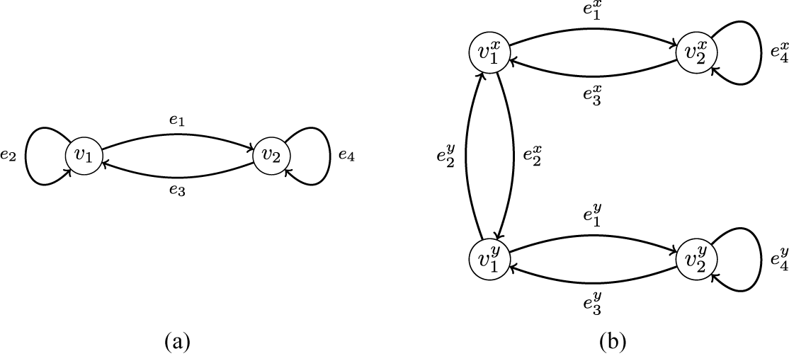
(a) The directed graph
 $(V,E)$
. (b) The projected directed graph
 $(\pi V,\pi E)$
associated with
 $(V,E)$
.

Let
 $\Psi =\{\psi _{e_i}:1\leq i\leq 4\}$
and
 $\{X_1,X_2\}$
be the family of graph-directed box-like self-affine set associated with
 $(V,E,\Psi )$
. See Figure 9 for the box-like self-affine GIFS
 $(V,E,\Psi )$
. For
 $i=1,2$
,
 $j=x,y$
, let
 $X_{i}^j=\pi _j(X_{i}).$
Write
 $\pi V=\{v_1^x,v_2^x,v_1^y,v_2^y\}$
,
 $\pi E=\{e_i^j:1\leq i\leq 4,\ j=x,y\}$
, and
 $$ \begin{align*} \pi \Psi= \{\psi_{e_i^j}=\pi_j\circ \psi_{e_i} \circ\pi_j^{-1}:i=1,3,4,\ j=x,y \}\cup \{\psi_{e_2^x}(\xi)=\tfrac{1}{3}\xi,\ \psi_{e_2^y}(\xi)=\tfrac{2}{3}\xi \}. \end{align*} $$
So,
 $\{X_{1}^x,X_{2}^x,X_{1}^y,X_{2}^y\}$
is a family of graph-directed self-similar set associated with
 $(\pi V,\pi E,\pi \Psi )$
(see Figure 8(b) for
 $(\pi V,\pi E)$
), that is,
 $$ \begin{align*} \begin{aligned} X_1^x= \psi_{e_1^x}(X_2^x)\cup \psi_{e_2^x}(X_1^y), \quad X_2^x= \psi_{e_3^x}(X_1^x)\cup \psi_{e_4^x}(X_2^x),\\ X_1^y= \psi_{e_1^y}(X_2^y)\cup \psi_{e_2^y}(X_1^x), \quad X_2^y= \psi_{e_3^y}(X_1^y)\cup \psi_{e_4^y}(X_2^y).\\ \end{aligned} \end{align*} $$
Images of
 $[0,1]^2$
under the first and second level iterations of map in GIFS
 $(V,E,\Psi )$
.

Let
 $\{\mu _{1},\mu _{2}\}$
be a graph-directed self-affine measure family associated with
 $(1/2,1/2,1/2,1/2)$
and
 $\{\mu _1^x,\mu _2^x,\mu _1^y,\mu _2^y\}$
be the family of projection measures. Note that
 $(\pi V, \pi E, \pi \Psi )$
is strongly connected and satisfies the graph-directed open set condition, so by [Reference Strichartz51], we have
 $$ \begin{align*} \tau_{\mu_1^x}(q)=\tau_{\mu_2^x}(q)=\tau_{\mu_1^y}(q)=\tau_{\mu_2^y}(q)=\beta(q), \end{align*} $$
where
 $\beta (q)$
is the unique solution of
 $$ \begin{align*} (\tfrac{1}{2})^q \cdot \bigg(\dfrac{1}{3}\bigg)^{\beta(q)}\cdot \rho \begin{pmatrix} 0& 2^{\beta(q)} & 1 & 0 \\ 1& 2^{\beta(q)} & 0 & 0 \\ 2^{\beta(q)} & 0 & 0 & 1 \\ 0& 0& 2^{\beta(q)} & 1 \end{pmatrix} =1. \end{align*} $$
Note that the spectral radius of the above
 $4\times 4$
matrix is
 $2^{\beta (q)}+1$
, so
 $\beta (q)$
is the unique solution of
 $$ \begin{align} 2^{\beta(q)}+1=2^q \cdot 3^{\beta(q)}. \end{align} $$
Proposition 3.8. For the measures
 $\{\mu _1,\mu _2\}$
in Example 3.7, we have
 $$ \begin{align*} \tau_{\mu_1}(q)=\tau_{\mu_2}(q)= \begin{cases} \beta(q) & \text{if } q\in [0,1],\\ \dfrac{(q-1)\log 4}{\log 2-\log 9} & \text{if }q\in (1,\infty), \end{cases} \end{align*} $$
where
 $\beta (q)$
is determined by (3.6).
Proof. The function matrix
 $\mathcal {G}^{(q)}_{x,y}$
defined in (2.6) becomes
 $$ \begin{align} (\tfrac{1}{2})^q \cdot \bigg(\dfrac{1}{3}\bigg)^{x+y}\cdot \begin{pmatrix} 0 & 0 & I & I \\ I & I & 0 & 0 \\ I & I & 0 & 0 \\ 0 & 0 & I & I \end{pmatrix} \cdot M \end{align} $$
with
 $$ \begin{align*}I= \begin{pmatrix} 1 & 0 \\ 0 & 1 \end{pmatrix}, \quad M=\text{diag} \bigg\{ \!\begin{pmatrix} t & 0 \\ 0 & s \\ \end{pmatrix}, \begin{pmatrix} 0 & s \\ t & 0 \\ \end{pmatrix}, \begin{pmatrix} s & 0 \\ 0 & t \\ \end{pmatrix}, \begin{pmatrix} t & 0 \\ 0 & s \\ \end{pmatrix} \!\bigg\}, \end{align*} $$
where
 $t=2^{x+\beta (q)}$
,
 $s=2^{y-\beta (q)}.$
From (3.7), it is easy to observe that the spectral radius of
 $\mathcal {G}^{(q)}_{x,y}$
equals
 $$ \begin{align} (\tfrac{1}{2})^q \cdot(\tfrac{1}{3})^{x+y} \cdot (2^{x+\beta(q)}+2^{y-\beta(q)} ). \end{align} $$
Using (3.6) and the definition of
 $\hat {\gamma }(q)$
in (2.7), it follows that
 $\hat {\gamma }(q) = \beta (q)$
. Since
 $t(q) = 2\beta (q)$
from (2.5), we have
 $\hat {\gamma }(q) \leq t(q)$
if and only if
 $\beta (q) \geq 0$
. By graphing the functions
 $2^\xi + 1$
and
 $2^q 3^\xi $
of
 $\xi $
, we observe that
 $\beta (q) \geq 0$
for
 $q \in [0,1]$
and
 $\beta (q) < 0$
for
 $q \in (1,\infty )$
. Therefore,
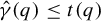 $\hat {\gamma }(q) \leq t(q)$
when
 $q \in [0,1]$
, and
 $\hat {\gamma }(q)> t(q)$
when
 $q \in (1,\infty )$
.
When
 $q\in [0,1]$
, using Theorem 2.3(a), we have
 $\gamma (q)=\hat {\gamma }(q)=\beta (q).$
It remains to consider the case
 $q\in (1,\infty )$
. For
 $x\in \mathbb {R}$
, let
 $y(x)$
be the unique solution such that (3.8) equals
 $1$
. By the theorem of implicit function, we have
 $$ \begin{align} y'(x)=-\frac{2^q 3^{x+y(x)}\log 3 -2^{x+\beta(q)}\log 2}{2^q 3^{x+y(x)}\log 3-2^{y(x)-\beta(q)}\log 2} \end{align} $$
and
 $y"(x)\geq 0$
(see also Lemma 6.16). Since
 $\beta (q)< 0$
,
 $y(0)=\hat {\gamma }(q)=\beta (q)$
and
 $y(x)$
is decreasing, there exists
 $x_0>0$
such that
 $$ \begin{align} x_0+\beta(q)=y(x_0)-\beta(q). \end{align} $$
Substituting this into (3.9) gives
 $y'(x_0)=-1,$
so that
 $x_0+y(x_0)$
is the minimum of
 $x+y(x)$
for
 $x\in \mathbb {R}$
. Based on (3.8) and (3.10), a calculation gives that
 $$ \begin{align*} x_0+y(x_0)=\frac{(q-1)\log 4}{\log 2-\log 9}, \quad x_0=\frac{(q-1)\log 2}{\log 2-\log 9} -\beta(q) < -\beta(q). \end{align*} $$
Using Theorem 2.3(b),
 $\gamma (q)= ({(q-1)\log 4})/({\log 2-\log 9}).$
Finally, the proposition follows by Theorem 2.2.
4 Pressure functions
Let
 $(V,E,\Psi )$
,
 ${\mathcal {P}}=(p_e)_{e\in E}$
and
 $\{\mu _v\}_{v \in V}$
be the same as before. First, we prove the existence of
 $L^q$
-spectra of measures in
 $\{\mu _v^x,\mu _v^y\}_{v\in V}.$
Proof of Proposition 2.1
Regard
 $\bar {V}=\{\mu _v^x,\mu _v^y\}_{v\in V}$
as a vertex set. Write
 $v_x=\mu _v^x$
,
 $v_y=\mu _v^y$
for short, that is,
 $\bar {V}=\{v_x,v_y\}_{v\in V}$
. For each
 $e\in E$
with
 $v=i(e),v'=t(e)$
, if
 $T_e$
is diagonal, we associate an edge
 $e_x$
so that
 $v_x\stackrel {e_x}{\longrightarrow } v^{\prime }_x$
(respectively
 $e_y$
so that
 $v_y \stackrel {e_y}{\longrightarrow } v^{\prime }_y$
); if
 $T_e$
is anti-diagonal, we associate an edge
 $e_x$
so that
 $v_x\stackrel {e_x}{\longrightarrow } v^{\prime }_y$
(respectively
 $e_y$
so that
 $v_y \stackrel {e_y}{\longrightarrow } v^{\prime }_x$
). Let
 $\psi _{e_x}=\pi _x(\psi _e)$
,
 $\psi _{e_y}=\pi _y(\psi _e)$
, and
 $p_{e_x}=p_{e_y}=p_e$
. Denote
 $\bar {E}=\{e_x,e_y\}_{e\in E}$
,
 $\bar {\Psi }=\{\psi _{e_x},\psi _{e_y}\}_{e\in E}$
, and
 $\bar {\mathcal {P}}=(p_{e_x},p_{e_y})_{e\in E}.$
Then,
 $(\bar {V}, \bar {E},\bar {\Psi })$
becomes a self-similar GIFS and
 $\{\mu _v^x,\mu _v^y\}_{v\in V}$
is the unique (but not necessarily strongly connected) graph-directed self-similar measure family associated with
 $(\bar {V},\bar {E},\bar {\Psi })$
and
 $\bar {\mathcal {P}}$
.
Consider the adjacency matrix
 $\mathcal {A}$
associated with
 $(\bar {V},\bar {E})$
, that is,
 $$ \begin{align*} \mathcal{A}(\bar{v},\bar{v}')= \begin{cases} 1 & \text{if there exists }\bar{e}\in \bar{E}\text{ such that }\bar{v}\stackrel{\bar{e}}{\to} \bar{v}', \\ 0 & \text{otherwise}. \end{cases} \end{align*} $$
When
 $\mathcal {A}$
is irreducible (that is, for
 $\bar {v},\bar {v}'\in \bar {V}, \mathcal {A}^k(\bar {v},\bar {v}')>0$
for some
 $k\in \mathbb {N}$
),
 $(\bar {V},\bar {E},\bar {\Psi })$
is a strongly connected self-similar GIFS. By Proposition 1.4, we know that all
 $\tau _{\mu _v^x}(q),\tau _{\mu _v^y}(q)$
exist and are equal to a common value.
When
 $\mathcal {A}$
is not irreducible, pick a pair
 $\bar {v}',\bar {v}"\in \bar {V}$
such that
 $$ \begin{align} \bar{v}'\nrightarrow\bar{v}". \end{align} $$
Define
 $$ \begin{align*} \begin{aligned} \bar{V}'&=\{\bar{v}\in \bar{V}: \bar{v}' \to \bar{v}\}, \quad \bar{V}"=\{\bar{v}\in \bar{V}: \bar{v}\to \bar{v}"\}. \end{aligned} \end{align*} $$
Clearly,
 $\bar {V}'\cap \bar {V}"=\emptyset .$
For each
 $v\in V$
, noticing that there exist
 $k_1,k_2 \in \mathbb {N}$
such that
 $$ \begin{align*} \mathcal{A}^{k_1}[\{\bar{v}'\},\{v_x,v_y\}] \text{ and } \mathcal{A}^{k_2}[\{v_x,v_y\},\{\bar{v}"\}] \text{ are non-zero matrices}, \end{align*} $$
using (4.1), we have
 $$ \begin{align*} 0=\mathcal{A}^{k_1+k_2}(\bar{v}',\bar{v}") \geq \mathcal{A}^{k_1}[\{\bar{v}'\},\{v_x,v_y\}] \cdot \mathcal{A}^{k_2}[\{v_x,v_y\},\{\bar{v}"\}]. \end{align*} $$
Thus,
 $$ \begin{align} \text{ either } v_x \in \bar{V}', v_y\in \bar{V}" \quad \text{ or }\quad v_x \in \bar{V}", v_y\in \bar{V}', \end{align} $$
which implies that
 $$ \begin{align} \bar{V}'\cup \bar{V}"=\bar{V}\quad \text{and} \quad \#\bar{V}'= \#\bar{V}"=\# \bar{V}/2. \end{align} $$
For the above v, we continue to consider two cases.
Case 1:
 $v_x \in \bar {V}', v_y\in {\bar {V}}^{\prime \prime }$
. We have
 $$ \begin{align*} v_x \nrightarrow v_y. \end{align*} $$
Define
 $$ \begin{align*} \bar{V}_v'=\{\bar{v}\in \bar{V}: v_x\to \bar{v}\},\quad \bar{V}_v"=\{\bar{v}\in \bar{V}: \bar{v}\to v_y\}. \end{align*} $$
We can see that
 $\bar {V}_v"\cap \bar {V}'= \emptyset $
, which by (4.3) immediately implies that
 $ \bar {V}_v'=\bar {V}'$
and
 $\bar {V}_v"=\bar {V}".$
Indeed, suppose that
 $\bar {V}_v"\cap \bar {V}'\neq \emptyset $
, then we have
 $$ \begin{align*} \bar{v}' \to \tilde{v} \to v_y \to \bar{v}" \quad \text{ for some } \tilde{v}\in \bar{V}_v"\cap \bar{V}', \end{align*} $$
which contradicts (4.1). Also, we have
 $\bar {v}'\in \bar {V}_v'=\bar {V}' $
, since if
 $\bar {v}'\in \bar {V}_v"$
, then
 $ \bar {v}'\to v_y \in \bar {V}', $
which contradicts
 $v_y \in \bar {V}"$
.
Case 2:
 $v_x\in \bar {V}",v_y\in \bar {V}'$
. Define
 $$ \begin{align*} \bar{V}_v'=\{\bar{v}\in \bar{V}: v_y\to \bar{v}\},\quad \bar{V}_v"=\{\bar{v}\in \bar{V}: \bar{v} \to v_x\}. \end{align*} $$
By a similar argument as above, we also have
 $\bar {v}'\in \bar {V}_v'=\bar {V}'$
and
 $\bar {V}_v"=\bar {V}"$
.
Thus, in both cases,
 $\mathcal {A}[\bar {V}',\bar {V}']$
is irreducible and
 $\mathcal {A}[\bar {V}',\bar {V}"] $
is a zero matrix.
Let
 $\kappa :\bar {V} \to \bar {V}$
be a one-to-one map defined as
 $\kappa (v_x)=v_y$
,
 $\kappa (v_y)=v_x$
, for any
 $v\in V$
. By (4.2) and the definition of
 $(\bar {V},\bar {E})$
, we know that
 $\kappa (\bar {V}')=\bar {V}"$
and
 $\mathcal {A}(\tilde {v},\tilde {v}')=\mathcal {A}({\kappa (\tilde {v}), \kappa (\tilde {v}')})$
. Thus,
 $\mathcal {A}[\bar {V}",\bar {V}"]$
is also irreducible and
 $\mathcal {A}[\bar {V}",\bar {V}']$
is a zero matrix.
Let
 $A= \bar {V}'$
and
 $B= \bar {V}"$
. Then,
 $A,B$
satisfy (2.3) and are two strongly connected self-similar measure families. By Proposition 1.4, (2.1) and (2.2) hold.
For
 $w=w_1\cdots w_k\in E^*$
, denote
 $p_w$
the product
 $p_{w_1} \cdots p_{w_k}$
,
 $T_w$
the product
 $T_{w_1} \cdots T_{w_k}$
, and
 $\psi _w$
the composition
 $\psi _{w_1} \circ \cdots \circ \psi _{w_k}$
. Let
 $$ \begin{align} c_w=|\pi_x(\psi_w([0,1]^2))| \quad \text{and} \quad d_w=|\pi_y(\psi_w([0,1]^2))| \end{align} $$
denote the width and height of the rectangle
 $\psi _w([0,1]^2)$
. Define
 $$ \begin{align} \pi_w= \begin{cases} \pi_x &\text{ if } c_w\geq d_w \text{ and } T_w \text{ is diagonal},\\ \pi_y &\text{ if } c_w <d_w \text{ and } T_w \text{ is diagonal},\\ \pi_y &\text{ if } c_w\geq d_w \text{ and } T_w \text{ is anti-diagonal},\\ \pi_x &\text{ if } c_w<d_w \text{ and } T_w \text{ is anti-diagonal}. \end{cases} \end{align} $$
For
 $q\geq 0,$
define
 $$ \begin{align} \tau_w(q)=\tau_{\pi_w(\mu_{t(w)})}(q). \end{align} $$
In other words,
 $\tau _w(q)$
is the
 $L^q$
-spectrum of the projection of
 $\mu _{t(w)}\circ \psi _{w}^{-1}$
onto the longest side of the rectangle
 $\psi _w([0,1]^2)$
, and it always equals either
 $\tau _A(q)$
or
 $\tau _B(q)$
by Proposition 2.1.
For
 $i=1,2$
, denote
 $\alpha _i(T)$
the ith singular value of a
 $2\times 2$
non-singular matrix T, that is, the positive square root of the ith (in decreasing order) eigenvalue of
 $T^*T$
, where
 $T^*$
is the transpose of T. For
 $w \in E^*$
, we write
 $\alpha _i(w)$
instead of
 $\alpha _i(T_w)$
for short. Now, we are able to give the definition of modified singular value function matrices (differs from the original definition [Reference Falconer9]), inspired by Fraser [Reference Fraser20, Reference Fraser21] dealing with the IFS setting.
Definition 4.1. (Modified singular value function matrices) For
 $s\in \mathbb {R}$
and
 $q\geq 0$
, define a function
 $\varphi ^{s,q}:E^*\to (0,\infty )$
by
 $$ \begin{align} \varphi^{s,q}(w)=p_w^q \alpha_1(w)^{\tau_w(q)} \alpha_2(w)^{s-\tau_w(q)}. \end{align} $$
For
 $k\in \mathbb {N}$
, define a
 $\#V \times \# V$
matrix
 $A_k^{s,q}$
with entries
 $$ \begin{align} A_k^{s,q}(v,v')=\sum_{w\in E^k: v \stackrel{w}{\rightarrow} v'} \varphi^{s,q}(w), \end{align} $$
where the empty sum is taken to be 0. Denote
 $A_0^{s,q}=\mathrm {id}$
, that is, the identity matrix, for convention. Call
 $\{A_k^{s,q}\}$
a sequence of modified singular value function matrices.
Lemma 4.2. For
 $w=w_1 \cdots w_k,w'=w^{\prime }_1 \cdots w^{\prime }_l\in E^*$
with
 $t(w)=i(w'),$
 $$ \begin{align*} \begin{aligned} &\tau_{x,w_k}(q)=\tau_{x,w^{\prime}_l}(q), \quad \tau_{y,w_k}(q)=\tau_{y,w^{\prime}_l}(q) \quad \text{if } T_{w'} \text{ is diagonal,}\\&\tau_{x,w_k}(q)=\tau_{y,w^{\prime}_l}(q), \quad \tau_{y,w_k}(q)=\tau_{x,w^{\prime}_l}(q) \quad \text{if } T_{w'} \text{ is anti-diagonal.} \end{aligned} \end{align*} $$
Proof. It suffices to prove that for
 $e,e'\in E$
with
 $t(e)=i(e')$
,
 $$ \begin{align} \begin{aligned} &\tau_{x,e}(q)=\tau_{x,e'}(q), \quad \tau_{y,e}(q)=\tau_{y,e'}(q) \quad \text{ if } T_{e'} \text{ is diagonal,}\\&\tau_{x,e}(q)=\tau_{y,e'}(q), \quad \tau_{y,e}(q)=\tau_{x,e'}(q) \quad \text{ if } T_{e'} \text{ is anti-diagonal.} \end{aligned} \end{align} $$
It follows from the proof of Proposition 2.1, we know that if
 $T_{e'}$
is diagonal, either
 $$ \begin{align*}\mu_{t(e)}^x ,\mu_{t(e')}^x\in A,\quad \mu_{t(e)}^y ,\mu_{t(e')}^y\in B,\end{align*} $$
or
 $$ \begin{align*}\mu_{t(e)}^x ,\mu_{t(e')}^x\in B,\quad \mu_{t(e)}^y ,\mu_{t(e')}^y\in A,\end{align*} $$
unless
 $\tau _A(q)=\tau _B(q)$
. By Proposition 2.1, (4.9) holds in this case. Also, if
 $T_{e'}$
is anti-diagonal, using a same argument, we still have (4.9).
Lemma 4.3. Let
 $s\in \mathbb {R},q\geq 0$
.
-
(a) For
$w, w'\in E^*$
with
$t(w)=i(w')$
, we have:-
(a1) if
$s<t(q)$
,
$\varphi ^{s,q}(ww')\leq \varphi ^{s,q}(w)\varphi ^{s,q}(w')$
; -
(a2) if
$s=t(q)$
,
$\varphi ^{s,q}(ww')= \varphi ^{s,q}(w)\varphi ^{s,q}(w')$
; -
(a3) if
$s>t(q)$
,
$\varphi ^{s,q}(ww')\geq \varphi ^{s,q}(w)\varphi ^{s,q}(w')$
.
-
-
(b) For
$k,l \in \mathbb {N}$
, we have:-
(b1) if
$s\leq t(q)$
,
$\Vert A_{k+l}^{s,q} \Vert \leq \Vert A_k^{s,q} \Vert \cdot \Vert A_l^{s,q} \Vert $
; -
(b2) if
$s> t(q)$
,
$\Vert A_{k+1}^{s,q}\Vert \gtrsim _{s,q}\Vert A_k^{s,q} \Vert $
and there exists
$J\in \mathbb {N}$
independent of
$k,l$
such that
$\max _{0\leq j\leq J}\Vert A_{k+j+l}^{s,q} \Vert \gtrsim _{s,q} \Vert A_k^{s,q} \Vert \cdot \Vert A_l^{s,q} \Vert $
.
-


Proof. (a1). Write
 $w=w_1 \cdots w_k$
and
 $w'=w^{\prime }_1 \cdots w_l'$
. By Proposition 2.1, we always have
 $$ \begin{align*} \tau_{x,e}(q)+\tau_{y,e}(q)=t(q) \quad \text{ for all } e\in E. \end{align*} $$
We only prove the case where
 $c_w\geq d_w$
, while the case
 $c_w<d_w$
is similar. We consider two possible subcases.
Case 1:
 $c_{ww'}=c_w c_{w'}, d_{ww'}=d_{w}d_{w'}$
. Note that in this case,
 $T_w$
is diagonal, so that
 $\tau _w(q)=\tau _{x,w_k}(q)$
. If
 $c_{w'}\geq d_{w'}$
and
 $c_{ww'}\geq d_{ww'}$
, using Lemma 4.2, we always have
 $$ \begin{align*} \tau_{w'}(q)=\tau_{ww'}(q)=\tau_{w}(q), \end{align*} $$
by checking
 $T_{w'}$
is diagonal or not separately. Thus,
 $$ \begin{align*} \frac{\varphi^{s,q}(ww')}{\varphi^{s,q}(w)\varphi^{s,q}(w')}=\frac{(c_w c_{w'})^{\tau_w(q)} (d_w d_{w'})^{s-\tau_w(q)}}{c_w^{\tau_w(q)} d_w^{s-\tau_w(q)} c_{w'}^{\tau_w(q)} d_{w'}^{s-\tau_w(q)}} =1. \end{align*} $$
If
 $c_{w'}<d_{w'}$
and
 $c_{ww'}\geq d_{ww'}$
, considering similarly as above, we always have
 $$ \begin{align*} \tau_{w'}(q)+\tau_{w}(q)=t(q) \quad \text{and}\quad \tau_{ww'}(q)=\tau_{w}(q). \end{align*} $$
Thus,
 $$ \begin{align*} \frac{\varphi^{s,q}(ww')}{\varphi^{s,q}(w)\varphi^{s,q}(w')}=\frac{(c_w c_{w'})^{\tau_w(q)} (d_w d_{w'})^{s-\tau_w(q)}}{c_w^{\tau_w(q)} d_w^{s-\tau_w(q)} d_{w'}^{t(q)-\tau_w(q)} c_{w'}^{s-t(q)+\tau_w(q)}}=\bigg(\frac{d_{w'}}{c_{w'}}\bigg)^{s-t(q)}\leq 1. \end{align*} $$
Otherwise,
 $c_{w'}<d_{w'}$
and
 $c_{ww'}<d_{ww'}$
, and similarly,
 $$ \begin{align*} \tau_{w'}(q)+\tau_{w}(q)=t(q) \quad \text{and}\quad \tau_{ww'}(q)=\tau_{w'}(q) \end{align*} $$
always holds. Thus,
 $$ \begin{align*} \frac{\varphi^{s,q}(ww')}{\varphi^{s,q}(w)\varphi^{s,q}(w')}=\frac{(d_w d_{w'})^{t(q)-\tau_w(q)} (c_w c_{w'})^{s-t(q)+\tau_w(q)}}{c_w^{\tau_w(q)} d_w^{s-\tau_w(q)} d_{w'}^{t(q)-\tau_w(q)} c_{w'}^{s-t(q)+\tau_w(q)}}=\bigg(\frac{c_{w}}{d_{w}}\bigg)^{s-t(q)}\leq 1. \end{align*} $$
In summary, property (a1) holds in this case.
Case 2:
 $c_{ww'}=c_w d_{w'}, d_{ww'}=d_w c_{w'}.$
In this case,
 $T_w$
is anti-diagonal, so
 $\tau _{w}(q)=\tau _{y,w_k}(q).$
If
 $d_{w'}\geq c_{w'}$
and
 $c_{ww'}\geq d_{ww'}$
, we always have
 $$ \begin{align*} \tau_{w'}(q)=\tau_{ww'}(q)=\tau_{w}(q), \end{align*} $$
so
 $$ \begin{align*} \frac{\varphi^{s,q}(ww')}{\varphi^{s,q}(w)\varphi^{s,q}(w')}=\frac{(c_w d_{w'})^{\tau_w(q)} (d_w c_{w'})^{s-\tau_w(q)}}{c_w^{\tau_w(q)} d_w^{s-\tau_w(q)} d_{w'}^{\tau_w(q)} c_{w'}^{s-\tau_w(q)}} =1. \end{align*} $$
If
 $d_{w'}<c_{w'}$
and
 $c_{ww'}\geq d_{ww'}$
, we always have
 $$ \begin{align*} \tau_{w'}(q)+\tau_{w}(q)=t(q) \quad \text{and} \quad \tau_{ww'}(q)=\tau_{w}(q), \end{align*} $$
so
 $$ \begin{align*} \frac{\varphi^{s,q}(ww')}{\varphi^{s,q}(w)\varphi^{s,q}(w')}=\frac{(c_w d_{w'})^{\tau_w(q)} (d_w c_{w'})^{s-\tau_w(q)}}{c_w^{\tau_w(q)} d_w^{s-\tau_w(q)} c_{w'}^{t(q)-\tau_w(q)} d_{w'}^{s-t(q)+\tau_w(q)}} =\bigg(\frac{c_{w'}}{d_{w'}}\bigg)^{s-t(q)}\leq 1. \end{align*} $$
Otherwise,
 $d_{w'}<c_{w'}$
and
 $c_{ww'}<d_{ww'}$
, and we always have
 $$ \begin{align*} \tau_{w'}(q)+\tau_{w}(q)=t(q) \quad \text{and} \quad \tau_{ww'}(q)=\tau_{w'}(q), \end{align*} $$
so
 $$ \begin{align*} \frac{\varphi^{s,q}(ww')}{\varphi^{s,q}(w)\varphi^{s,q}(w')}=\frac{(d_w c_{w'})^{t(q)-\tau_w(q)} (c_w d_{w'})^{s-t(q)+\tau_w(q)}}{c_w^{\tau_w(q)} d_w^{s-\tau_w(q)} c_{w'}^{t(q)-\tau_w(q)} d_{w'}^{s-t(q)+\tau_w(q)}} =\bigg(\frac{c_{w}}{d_{w}}\bigg)^{s-t(q)}\leq 1. \end{align*} $$
So, in summary, property (a1) also holds in this case.
The proofs of properties (a2) and (a3) follow by using a similar argument as above.
(b1). If
 $s\leq t(q)$
, then
 $$ \begin{align*} \begin{aligned} \Vert A_{k+l}^{s,q} \Vert &= \sum_{v,v'\in V} A_{k+l}^{s,q}(v,v') =\sum_{v,v'\in V} \sum_{w\in E^{k+l}: v\stackrel{w}{\rightarrow}v'} \varphi^{s,q}(w)\\ &\leq \sum_{v,v'\in V} \sum_{v"\in V} \sum_{w\in E^k:v\stackrel{w}{\rightarrow} v"} \sum_{w'\in E^l:v"\stackrel{w'}{\rightarrow} v'} \varphi^{s,q}(w) \varphi^{s,q}(w') \ \ \text{by properties~(a1) and (a2)}\\ &=\sum_{v,v'\in V} \sum_{v"\in V} A_k^{s,q}(v,v") A_l^{s,q}(v",v') =\sum_{v,v'\in V}( A_k^{s,q}\cdot A_l^{s,q} )(v,v') \\ &= \Vert A_k^{s,q} \cdot A_l^{s,q} \Vert \leq \Vert A_k^{s,q} \Vert \Vert A_l^{s,q} \Vert. \end{aligned} \end{align*} $$
(b2). If
 $s> t(q)$
, for
 $k\geq 0$
, we have
 $A_{k+1}^{s,q}\geq A_k^{s,q} A^{s,q}_1$
by the same argument as above and using property (a3). Denote
 $C=\min _{v\in V} \sum _{v'\in V} A_1^{s,q}(v,v')>0$
. It is direct to see that
 $\Vert A_k^{s,q} A_1^{s,q} \Vert \geq C \Vert A_k^{s,q} \Vert $
, which gives the first part of item (b2).
Supposed the second part of property (b2) is not true, that is, for any
 $\epsilon>0$
and
 $J\in \mathbb {N}$
, there exist
 $k,l\in \mathbb {N}$
such that
 $ \Vert A_{k+j+l}^{s,q} \Vert \leq \epsilon \Vert A_k^{s,q} \Vert \Vert A_l^{s,q} \Vert $
for all
 $0\leq j\leq J$
. Let
 $u=(1,\ldots , 1)$
be a row vector in
 $\mathbb {R}^{\#V}$
. Noticing that
 $A_{k+j+l}^{s,q} \geq A_k^{s,q} \cdot A_j^{s,q} \cdot A_l^{s,q}$
, we have
 $$ \begin{align*} u A_k^{s,q} A_j^{s,q} A_l^{s,q} u^* \leq \Vert A_{k+j+l}^{s,q} \Vert \leq \epsilon \Vert A_k^{s,q} \Vert \Vert A_l^{s,q} \Vert. \end{align*} $$
Define two non-negative unit row vectors
 ${u'}=({u\cdot A_k^{s,q}})/({\Vert A_k^{s,q}\Vert })$
and
 ${u"}={((A_l^{s,q} u^*)^*)}/ {(\Vert A_l^{s,q} \Vert )}$
, then
 $$ \begin{align*} {u'} A_j^{s,q} {u"}^* \leq \epsilon \quad \text{ for all } 0\leq j\leq J. \end{align*} $$
Take two sequences
 $\{\epsilon _n\}\to 0$
and
 $\{J_n\} \to \infty $
. Then, for each n, there exist two non-negative unit row vectors
 $u_n',u_n"$
such that
 $$ \begin{align*} u_n' A_j^{s,q} {u_n"}^* \leq \epsilon_n\quad \text{ for all } 0\leq j\leq J_n. \end{align*} $$
Let
 $(u',u")$
be a limit point of
 $\{(u_n',u_n")\}_{n\in \mathbb {N}}$
, then we have
 $$ \begin{align*} u' A_j^{s,q} u^{\prime\prime*}=0 \quad \text{ for all } j\geq 0. \end{align*} $$
Noticing that
 $u',u"$
are two non-negative unit row vectors and all
 $A_j^{s,q} $
are non-negative matrices, we have that there exist
 $v,v'\in V$
such that
 $A_j^{s,q}(v,v')=0$
for all
 $j\geq 0$
. This contradicts the strong connectivity of the directed graph
 $(V,E)$
.
Remark 4.4. The property (b2) was summarized by Feng [Reference Feng16], which was fundamental for random matrix product and multifractal analysis, see e.g. [Reference Feng and Käenmäki17, Reference Käenmäki and Reeve26].
Lemma 4.5. (Pressure function)
Define a function
 $P:\mathbb {R}\times [0,\infty ) \to [0,\infty )$
by
 $$ \begin{align} P(s,q)=\lim_{k\to \infty} \Vert A_k^{s,q} \Vert^{1/k}. \end{align} $$
The definition is well defined. Call P a pressure function associated with
 $(V,E,\Psi )$
and
 $\mathcal {P}$
.
Proof. It suffices to prove the existence of a limit in (4.10).
For
 $q\geq 0$
,
 $s\leq t(q)$
, the limit exists by Lemma 4.3(b1) and the standard property of submultiplicative sequences.
For
 $s> t(q)$
, by Lemma 4.3(b2), there exist
 $C>0$
(depending on
 $s,q$
) and
 $J\in \mathbb {N}$
such that
 $$ \begin{align*} \begin{aligned} \Vert A_{k+1}^{s,q} \Vert &\geq C \Vert A_k^{s,q} \Vert\qquad\quad\ \ \ \text{for all } k\geq 0, \\ \max_{0\leq j\leq J} \Vert A_{k+j+l}^{s,q} \Vert &\geq C \Vert A_k^{s,q} \Vert \Vert A_l^{s,q} \Vert \quad \text{for all } k,l\geq 0. \end{aligned} \end{align*} $$
Therefore, there exists
 $C'>0$
such that
 $\Vert A_{k}^{s,q} \Vert \Vert A_l^{s,q} \Vert \leq C^{-1}\sum _{0\leq j\leq J}\Vert A_{k+j+l}^{s,q} \Vert \leq C' \Vert A_{k+J+l}^{s,q}\Vert $
. This implies that the sequence
 $\{({1}/{C'}) \Vert A_{k-J}^{s,q} \Vert \}_{k\geq J}$
is supermultiplicative, so the limit (4.10) exists.
Write
 $$ \begin{align} \begin{aligned} \alpha_*&=\min \{\alpha_2(e):e\in E\} =\min \{a_e,b_e:e\in E\}, \\ \alpha^*&=\max \{\alpha_1(e):e\in E\}=\max \{a_e,b_e:e\in E\},\\ p_*&=\min \{p_e:e\in E\}, \\ p^*&=\max \{p_e:e\in E\}. \end{aligned} \end{align} $$
Recall that the
 $L^q$
-spectra of a measure is Lipschitz continuous on
 $[\unicode{x3bb} ,\infty )$
for all
 $\unicode{x3bb}>0$
. Let
 $L_\unicode{x3bb} $
be the larger of the two Lipschitz constants corresponding to
 $\tau _A$
and
 $\tau _B$
on
 $[\unicode{x3bb} ,\infty )$
.
Lemma 4.6. For
 $t,r\in \mathbb {R}$
and
 $\unicode{x3bb}>0$
, define
 $$ \begin{align*} U(t,r,\unicode{x3bb})=\min \{\alpha_*^tp_*^r, \alpha_*^tp^{*r}, \alpha^{*t}p_*^r, \alpha^{*t}p^{*r}\}\bigg(\frac{\alpha^*}{\alpha_*}\bigg)^{\min \{-L_\unicode{x3bb} r,0\}} \end{align*} $$
and
 $$ \begin{align*} V(t,r,\unicode{x3bb})=\max \{\alpha_*^tp_*^r, \alpha_*^tp^{*r}, \alpha^{*t}p_*^r, \alpha^{*t}p^{*r}\}\bigg(\frac{\alpha^*}{\alpha_*}\bigg)^{\max \{-L_\unicode{x3bb} r,0\}}. \end{align*} $$
Then, for all
 $s,t\in \mathbb {R}$
,
 $\unicode{x3bb}>0$
,
 $q\geq \unicode{x3bb} $
, and
 $r\geq \unicode{x3bb} -q$
,
 $$ \begin{align*} U(t,r,\unicode{x3bb}) P(s,q) \leq P(s+t,q+r) \leq V(t,r,\unicode{x3bb}) P(s,q), \end{align*} $$
and for
 $s,t\in \mathbb {R}$
,
 $$ \begin{align*} \min\{\alpha_*^t,\alpha^{*t}\} P(s,0)\leq P(s+t,0) \leq \max\{ \alpha_*^t,\alpha^{*t} \} P(s,0). \end{align*} $$
Also, for all
 $s\in \mathbb {R}$
and
 $q\geq 0$
,
 $$ \begin{align*} P(s,q)\leq p^{*q}P(s,0). \end{align*} $$
Consequently, we have:
-
(a) P is continuous on
$\mathbb {R}\times (0,\infty )$
and on
$\mathbb {R}\times \{0\}$
; -
(b) P is strictly decreasing in
$s\in \mathbb {R}$
; -
(c) for each
$q\geq 0$
, there exists a unique
$s\in \mathbb {R}$
such that
$P(s,q)=1$
.


Proof. This is essentially the same as [Reference Fraser21, Lemma 2.3].
Remark 4.7. For
 $q\geq 0$
, we refer to
 $\gamma (q)$
as the unique
 $s\in \mathbb {R}$
satisfying
 $P(s,q)=1$
. In Theorem 2.2, we will prove that
 $\tau _{\mu _v}(q)=\gamma (q)$
for all
 $v\in V$
under the ROSC.
5 Proof of Theorem 2.2
In this section, we are going to prove Theorem 2.2. The main idea is based on Fraser’s work [Reference Fraser21] for the IFS setting. Let
 $(V,E,\Psi )$
,
 $\mathcal {P}$
, and
 $\{\mu _v\}_{v\in V}$
be the same as before. Let
 $\gamma (q)$
be the function determined by
 $P(\gamma (q),q)=1$
(see Remark 4.7), where P is the pressure function introduced in Lemma 4.5.
Denote the collection of all infinite admissible words by
 $$ \begin{align*} E^\infty=\{\omega=\omega_1\omega_2\cdots:t(\omega_{i-1})=i(\omega_i) \text{ for all } i>1\}. \end{align*} $$
For
 $w=w_1\cdots w_k\in E^*$
, denote
 $[w]=\{\omega =\omega _1 \omega _2 \cdots \in E^\infty :\omega _i=w_i \text { for } 1\leq i\leq k\}$
the cylinder set of w. For
 $\delta>0$
, write
 $$ \begin{align*} E^*_\delta=\{w=w_1 \cdots w_k \in E^*: \alpha_2(w)<\delta \leq \alpha_2(w_1 \cdots w_{k-1})\}. \end{align*} $$
Roughly speaking,
 $E^*_\delta $
consists of all
 $w\in E^*$
for which the shortest side of the rectangle
 $\psi _w([0,1]^2)$
is comparable to
 $\delta $
. So, for each
 $w=w_1 \cdots w_k\in E^*_\delta $
, we have
 $$ \begin{align} \delta>\alpha_2(w) \geq \alpha_2(w_1\cdots w_{k-1}) \alpha_2(w_k) \geq \alpha_* \delta, \end{align} $$
where
 $\alpha _*$
is defined in (4.11). It is easy to see that
 $E^*_\delta $
is a finite partition of
 $E^\infty $
, that is,
 $\#E_\delta ^*<\infty $
and
 $$ \begin{align*} E^\infty=\bigcup_{w\in E^*_\delta} [w], \end{align*} $$
where the union is disjoint.
Before proving Theorem 2.2, we need the following lemma, which is adapted from [Reference Fraser21, Lemma 7.1].
Lemma 5.1. Let
 $q\geq 0$
and
 $\delta>0$
.
-
(a) For
$s> \gamma (q)$
,
$$ \begin{align*} \sum_{w\in E^*_\delta} \varphi^{s,q}(w) \lesssim_{s,q} 1. \end{align*} $$
-
(b) For
$s<\gamma (q)$
,
$$ \begin{align*} \sum_{w\in E^*_\delta} \varphi^{s,q}(w) \gtrsim_{s,q} 1. \end{align*} $$


Proof. (a) For
 $s>\gamma (q)$
, it follows that
 $$ \begin{align*} \sum_{w\in E^*_\delta}\varphi^{s,q}(w)\leq \sum_{w\in E^*}\varphi^{s,q}(w) =\sum_{k\geq 1}\sum_{w\in E^k} \varphi^{s,q}(w) =\sum_{k\geq 1} \Vert A^{s,q}_k \Vert <\infty, \end{align*} $$
since
 $\lim _{k\to \infty } \Vert A_k^{s,q} \Vert ^{1/k} =P(s,q)<1$
by Lemma 4.6.
(b) We divide the proof into two cases,
 $s\leq t(q)$
or
 $s>t(q)$
.
Case 1:
 $s\leq t(q).$
We will prove
 $\sum _{w\in E^*_\delta } \varphi ^{s,q}(w)\geq 1$
through a contradiction argument. Suppose
 $$ \begin{align} \sum_{w\in E^*_\delta} \varphi^{s,q}(w)< 1. \end{align} $$
Fix a
 $\delta>0$
. Note that for all
 $w\in E^*$
, by Lemma 4.3 and (5.2), we have
 $$ \begin{align} \sum_{w'\in E^*_\delta:t(w)=i(w')} \varphi^{s,q}(ww') \leq \varphi^{s,q}(w) \sum_{w'\in E^*_\delta} \varphi^{s,q}(w')<\varphi^{s,q}(w). \end{align} $$
Now, for large enough
 $k\in \mathbb {N}$
, define
 $$ \begin{align*} E^k_\delta =\{w=w^{(1)} \cdots w^{(m)}\in E^*:w^{(j)}\in E^*_\delta, \text{ with } |w|>k \text{ and } |w^{(1)}\cdots w^{(m-1)}|\leq k\}. \end{align*} $$
Clearly,
 $E^k_\delta $
is a finite partition of
 $E^\infty $
. Repeatedly using (5.3), for large enough k, we have
 $$ \begin{align} \sum_{w\in E^k_\delta} \varphi^{s,q}(w)<1. \end{align} $$
Let
 $n_0(\delta )=\max \{|w|:w\in E^*_\delta \}$
. For
 $w\in E^{k+n_0(\delta )}$
, we have
 $w=w^{(1)}w^{(2)}$
for some
 $w^{(1)}\in E^k_\delta $
,
 $w^{(2)} \in E^*\cup \{\emptyset \}$
with
 $t(w^{(1)})=i(w^{(2)})$
and
 $|w^{(2)}|< n_0(\delta )$
. Let
 $c(\delta )=\max \{\varphi ^{s,q}(w):|w|<n_0(\delta )\}>0$
, which is independent of k. Since there are at most
 $(\#E)^{n_0(\delta )}$
choices of
 $w^{(2)}\in E^*\cup \{\emptyset \}$
, by Lemma 4.3 and using (5.4), we have
 $$ \begin{align*} \Vert A^{s,q}_{k+n_0(\delta)} \Vert =\sum_{w\in E^{k+n_0(\delta)}}\varphi^{s,q}(w)\leq (\#E)^{n_0(\delta)} c_\delta \sum_{w\in E^k_\delta} \varphi^{s,q}(w) <(\#E)^{n_0(\delta)} c_\delta. \end{align*} $$
It follows that
 $$ \begin{align*} P(s,q)=\lim_{k\to \infty}\Vert A_k^{s,q} \Vert^{1/k} \leq 1, \end{align*} $$
which gives that
 $s\geq \gamma (q)$
by Lemma 4.6, and this is a contradiction.
Case 2:
 $s>t(q)$
. Noticing that the directed graph
 $(V,E)$
is strongly connected, for each pair
 $v,v'\in V$
, define
 $L(v,v'):=\min \{|w|:w\in E^*,v \stackrel {w}{\rightarrow } v'\}$
and let
 $L:=\max \{L(v,v'):v,v'\in V\}$
be the maximal length of shortest paths between any two vertices.
Let
 $C=\min \{\varphi ^{s,q}(w):|w|\leq L\}>0.$
Replace the matrix norm
 $\Vert \cdot \Vert $
with the maximum row sum norm
 $\Vert \cdot \Vert _1$
, that is,
 $\Vert A \Vert _1=\max _{1\leq i\leq N}\sum _{1\leq j\leq N} |a_{ij}|$
for an
 $N\times N$
matrix
 $A=(a_{ij})_{1\leq i,j\leq N}$
. Due to the equivalence of matrix norms and
 $s<\gamma (q)$
, it follows that
 $\Vert A_k^{s,q} \Vert _1 \to \infty $
as
 $k\to \infty $
. So, we could find
 $k\in \mathbb {N}$
and
 $v_0\in V$
such that
 $$ \begin{align} \sum_{w\in E^k:i(w)=v_0} \varphi^{s,q}(w)=\Vert A_k^{s,q}\Vert_1>1/C. \end{align} $$
Fix such k and
 $v_0$
. For small enough
 $\delta>0$
, let
 $$ \begin{align*} &E_{k,\delta} = \big\{ w^{(1)} \tilde{w}^{(1)} w^{(2)} \tilde{w}^{(2)}\cdots \tilde{w}^{(m-1)} w^{(m)}\in E^*: |w^{(j)}| =k, i(w^{(j)})=v_0, t(w^{(j)})\\ & \stackrel{ \tilde{w}^{(j)}}{\longrightarrow} v_0, |\tilde{w}^{(j)} |=L(t(w^{(j)}),v_0) ,\alpha_2(w^{(1)} \tilde{w}^{(1)}\!\cdots w^{(m)}) <\delta \leq \alpha_2(w^{(1)} \tilde{w}^{(1)}\!\cdots w^{(m-1)})\big\}. \end{align*} $$
We can directly check that the cylinder sets of elements in
 $E_{k,\delta }$
are all disjoint (but
 $E_{k,\delta }$
is not a finite partition of
 $E^\infty $
). For any
 $w\in E^*$
, by Lemma 4.3 and using (5.5), we have
 $$ \begin{align} \sum_{w'\in E^{L(t(w),v_0)}} \sum_{w"\in E^{k}:i(w")=v_0} \!\varphi^{s,q}(ww'w")\geq C \varphi^{s,q}(w)\!\! \sum_{w"\in E^k:i(w")=v_0} \!\varphi^{s,q}(w")>\varphi^{s,q}(w). \end{align} $$
Repeatedly using (5.6), we have
 $$ \begin{align} \sum_{w\in E_{k,\delta}} \varphi^{s,q}(w)>1/C. \end{align} $$
Also, note that for
 $w=w^{(1)} \tilde {w}^{(1)} \cdots w^{(m)}\in E_{k,\delta }$
,
 $$ \begin{align} \delta>\alpha_2(w) \geq \alpha_2(w^{(1)} \tilde{w}^{(1)}\cdots w^{(m-1)}) \alpha_2(\tilde{w}^{(m-1)} w^{(m)}) \geq \alpha_*^{L+k} \delta. \end{align} $$
Take
 $\delta '=\alpha _*^{L+k} \delta $
, then for
 $w\in E_{\delta '}^*$
, by (5.1), we have
 $$ \begin{align} \alpha_*^{L+k} \delta =\delta'>\alpha_2(w) \geq \alpha_* \delta' =\alpha_*^{L+k+1} \delta. \end{align} $$
For
 $w \in E^*_{\delta '}$
, if w has a prefix in
 $E_{k,\delta }$
, we can write
 $w=w'w"$
with
 $t(w')=i(w")$
for some
 $w'\in E_{k,\delta }$
and
 $w" \in E^*$
. Combining (5.8), (5.9), and
 $\alpha _2(w'w") \leq \alpha _2(w')\alpha _1(w") \leq \alpha _2(w') \alpha ^{*|w"|}$
, we have
 $$ \begin{align*} \alpha_2(w') <\delta \alpha_*^{L+k+1} \alpha_*^{-L-k-1} \leq \alpha_2(w) \alpha_*^{-L-k-1} \leq \alpha_2(w') \alpha^{*|w"|} \alpha_*^{-L-k-1}, \end{align*} $$
which gives that
 $|w"|\leq (L+k+1) ({\log \alpha _*}/{\log \alpha ^*})$
.
Let
 $C'=\min \{\varphi ^{s,q}(w):|w|\leq (L+k+1) ({\log \alpha _*}/{\log \alpha ^*}) \}>0$
. Then, by (5.7) and Lemma 4.3, we have
 $$ \begin{align*} \sum_{w\in E^*_{\delta'}} \varphi^{s,q}(w) &\geq \sum_{w\in E^*_{\delta'}:w \text{ has a prefix in } E_{k,\delta}} \varphi^{s,q}(w) \\ &\geq C' \sum_{w\in E_{k,\delta}} \varphi^{s,q}(w)>C'/C. \end{align*} $$
The constant
 $C'/C$
only depends on k and the choice of k depends on
 $s,q$
.
Before proceeding, we mention a fact [Reference Fraser21, Lemma 4.1] that will be used in the proof of Theorem 2.2. For
 $k\in \mathbb {N}, a_1,\ldots , a_k\geq 0$
, we have
 $$ \begin{align} \kern-17pt\bigg(\sum_{i=1}^k a_i\bigg)^q &\leq \sum_{i=1}^{k} a_i^q \quad\text{for }q\in [0,1], \end{align} $$
 $$ \begin{align} \kern-10pt\bigg(\sum_{i=1}^k a_i\bigg)^q &\geq \sum_{i=1}^{k} a_i^q \quad\text{for }q\in [1,\infty), \end{align} $$
 $$ \begin{align} \bigg(\sum_{i=1}^k a_i\bigg)^q &\asymp_{k,q} \sum_{i=1}^{k} a_i^q \quad\text{for }q\in [0,\infty). \end{align} $$
Proof of Theorem 2.2
For
 $q\geq 0$
and
 $\delta>0$
, recall that we use
 $\mathcal {M}_\delta $
to denote the collection of
 $\delta $
-mesh on
 $\mathbb {R}^2$
, and for a measure
 $\mu $
, we write
 $\mathcal {D}_\delta ^q(\mu )=\sum _{Q\in \mathcal {M}_\delta } \mu (Q)^q$
.
We first prove part (c) under the assumption ROSC. First of all, due to the ROSC, there exists
 $M>0$
independent of
 $\delta $
such that for each
 $Q\in \mathcal {M}_\delta $
, we have
 $$ \begin{align} \#\{w\in E^*_\delta:\mu_{t(w)}\circ \psi^{-1}_w ( Q\cap \psi_w([0,1]^2))>0\} \leq M. \end{align} $$
Combining this and (5.12), for
 $v\in V$
, we have
 $$ \begin{align} \mathcal{D}_\delta^q(\mu_v) & =\sum_{Q\in \mathcal{M}_\delta} \mu_v(Q)^q =\sum_{Q\in \mathcal{M}_\delta} \bigg(\sum_{w\in E^*_\delta:i(w)=v} p_w \mu_{t(w)}\circ \psi_w^{-1}(Q\cap \psi_w([0,1]^2))\bigg)^q\nonumber\\ & \asymp_{q} \sum_{Q\in \mathcal{M}_\delta} \sum_{w\in E^*_\delta:i(w)=v} p_w^q \mu_{t(w)}\circ \psi_w^{-1}(Q\cap \psi_w([0,1]^2))^q\nonumber\\ & =\sum_{w\in E^*_\delta:i(w)=v} p_w^q \mathcal{D}_\delta^q(\mu_{t(w)}\circ \psi_w^{-1}). \end{align} $$
Using (5.12) again and the definition of
 $\pi _w$
in (4.5), we have
 $$ \begin{align*} \mathcal{D}_\delta^q(\mu_{t(w)}\circ\psi_w^{-1})\asymp_q \mathcal{D}^q_{\delta/\alpha_1(w)} (\pi_w(\mu_{t(w)})). \end{align*} $$
So, (5.14) becomes
 $$ \begin{align} \mathcal{D}_\delta^q(\mu_v) \asymp_q \sum_{w\in E^*_\delta:i(w)=v} p_w^q \mathcal{D}^q_{\delta/\alpha_1(w)} (\pi_w(\mu_{t(w)})). \end{align} $$
However, recall that for
 $q\geq 0$
,
 $w\in E^*$
,
 $\tau _w(q)=\tau _{\pi _w(\mu _{t(w)})}(q)$
and equals either
 $\tau _A(q)$
or
 $\tau _B(q)$
. By the definition of
 $L^q$
-spectra, for all
 $w\in E^*$
,
 $\epsilon>0$
,
 $q\geq 0$
, small enough
 $\delta>0$
, we have
 $$ \begin{align} \delta^{-\tau_w(q)+\epsilon/2} \lesssim_{\epsilon,q} \mathcal{D}_\delta^q(\pi_w(\mu_{t(w)})) \lesssim_{\epsilon,q} \delta^{-\tau_w(q)-\epsilon/2}. \end{align} $$
For each fixed
 $v\in V$
, combining (5.15), (5.16), and Lemma 5.1, noticing that
 $\delta \asymp \alpha _2(w)$
for
 $w\in E_\delta ^*$
, we have
 $$ \begin{align} \delta^{\gamma(q)+\epsilon}\mathcal{D}_\delta^q(\mu_v) &\lesssim_q \delta^{\gamma(q)+\epsilon} \sum_{w\in E^*_\delta:i(w)=v} p_w^q \mathcal{D}^q_{\delta/\alpha_1(w)} (\pi_w(\mu_{t(w)})) \notag\\ &\lesssim_{\epsilon,q} \delta^{\gamma(q)+\epsilon} \sum_{w\in E^*_\delta:i(w)=v} p_w^q \bigg( \frac{\delta}{\alpha_1(w)}\bigg ) ^{-\tau_w(q)-\epsilon/2} \notag\\ &\lesssim_{\epsilon,q} \sum_{w\in E^*_\delta:i(w)=v} p_w^q \alpha_1(w)^{\tau_w(q)} \alpha_2(w)^{\gamma(q)+{\epsilon}/{2}-\tau_w(q)} \cdot \alpha_1(w)^{{\epsilon}/{2}} \notag\\ &\leq \sum_{w\in E^*_\delta:i(w)=v} \varphi^{\gamma(q)+{\epsilon}/{2},q}(w) \notag\\ &\lesssim_{\epsilon,q} 1. \end{align} $$
Letting
 $\delta ,\epsilon \to 0$
, we have
 $\overline {\tau }_{\mu _v}(q)\leq \gamma (q)$
.
A similar argument will imply
 $\gamma (q) \leq \underline {\tau }_{\mu _v}(q)$
. Indeed, noting that for any
 $v'\in V$
, it always holds that
 $v \stackrel {w}{\rightarrow } v'$
for some w and
 $\mu _v \geq p_w \mu _{v'}\circ \psi _w^{-1}$
, and we have
 $ \mathcal {D}_\delta ^q(\mu _v)\gtrsim _q \mathcal {D}_\delta ^q(\mu _{v'})$
. Using this, still by (5.15), (5.16), and Lemma 5.1, if the ROSC holds, we have
 $$ \begin{align*} \delta^{\gamma(q)-\epsilon}\mathcal{D}_\delta^q(\mu_v)&\gtrsim_q \sum_{v'\in V}\delta^{\gamma(q)-\epsilon}\mathcal{D}_\delta^q(\mu_{v'})\\ &\gtrsim_q \delta^{\gamma(q)-\epsilon} \sum_{w\in E^*_\delta} p_w^q \mathcal{D}^q_{\delta/\alpha_1(w)} (\pi_w(\mu_{t(w)}))\\ &\gtrsim_{\epsilon,q} \delta^{\gamma(q)-\epsilon} \sum_{w\in E^*_\delta} p_w^q \bigg( \frac{\delta}{\alpha_1(w)} \bigg) ^{-\tau_w(q)+{\epsilon}/{2}} \\ &\gtrsim_{\epsilon,q} \sum_{w\in E^*_\delta} p_w^q \alpha_1(w)^{\tau_w(q)} \alpha_2(w)^{\gamma(q)-{\epsilon}/{2}-\tau_w(q)} \cdot \alpha_1(w)^{-{\epsilon}/{2}} \\ &\geq \sum_{w\in E^*_\delta} \varphi^{\gamma(q)-{\epsilon}/{2},q}(w)\\ &\gtrsim_{\epsilon,q} 1, \end{align*} $$
which yields that
 $\gamma (q)\leq \underline {\tau }_{\mu _v}(q)$
.
Therefore, for each
 $v\in V$
,
 $\tau _{\mu _v}(q)$
exists and equals
 $ \gamma (q)$
for all
 $q\geq 0$
.
We now turn to the proofs of parts (a) and (b). In these cases, it is unknown whether (5.13) holds, as the ROSC is not required. Nevertheless, for
 $q\in [0,1]$
, using (5.10) in place of (5.12) implies that the ‘
 $\asymp _q$
’ in (5.14) and (5.15) can be replaced by ‘
 $\leq $
’ and ‘
 $\lesssim _q$
’, respectively. This is sufficient to establish (5.17), thus proving part (a). The proof of part (b) for
 $q\in [1,\infty )$
follows similarly, with (5.12) replaced by (5.11).
6 Closed forms
In this section, we will prove Theorem 2.3 and Corollaries 2.4, 2.6, 2.7, and 2.9. We always let
 $(V,E,\Psi )$
be a strongly connected planar box-like self-affine GIFS. Let
 $\mathcal {P}$
,
 $\{\mu _v\}_{v\in V}$
be the associated positive vector and measures as before. We will present the closed form expression for
 $\gamma (q)$
(
 $L^q$
-spectra of
 $\{\mu _v\}_{v\in V}$
by Theorem 2.2 under the ROSC). Throughout this section, we always fix a
 $q\geq 0$
, so when we define new variables, we may omit q.
6.1 Notation and lemmas
For
 $x,y\in \mathbb {R}$
,
 $e,e'\in E$
, we define a
 $2\times 2$
matrix
 $G_{x,y,e,e'}^{(q)}$
by
 $$ \begin{align*} G^{(q)}_{x,y,e,e'} = \begin{cases} \!\!\!\!\!&\begin{aligned} \begin{pmatrix} p_{e'}^q a_{e'}^{x+\tau_{x,e'}(q)} b_{e'}^{y-\tau_{x,e'}(q)} & 0 \\ 0 & p_{e'}^q b_{e'}^{x+\tau_{y,e'}(q)} a_{e'}^{y-\tau_{y,e'}(q)} \\ \end{pmatrix} \hspace{2.45cm}\\ \text{ if } t(e)=i(e') \text{ and }T_{e'} \text{ is diagonal, } \end{aligned} \\ \!\!\!\!\!&\begin{aligned} \begin{pmatrix} 0 & p_{e'}^q a_{e'}^{x+\tau_{y,e'}(q)} b_{e'}^{y-\tau_{y,e'}(q)} \\ p_{e'}^q b_{e'}^{x+\tau_{x,e'}(q)} a_{e'}^{y-\tau_{x,e'}(q)} &0 \\ \end{pmatrix} \hspace{3cm} \\ \text{ if } t(e)=i(e') \text{ and } T_{e'} \text{ is anti-diagonal,} \end{aligned} \\ \!\!\!\!\!&\begin{pmatrix} 0 & 0 \\ 0 &0 \\ \end{pmatrix} \hspace{3.65cm} \text{otherwise. } \end{cases} \end{align*} $$
Denote
 $\{e(1),e(2)\}\times \{e'(1),e'(2)\}$
as the collection of indices of matrix
 $G^{(q)}_{x,y,e,e'}$
. We introduce a
 $\# E \times \# E$
block matrix
 $\mathcal {G}_{x,y}^{(q)}$
with entries defined by
 $$ \begin{align*} \mathcal{G}_{x,y}^{(q)}[\{e(1),e(2)\},\{e'(1),e'(2)\}] = G_{x,y,e,e'}^{(q)}. \end{align*} $$
Let
 $\hat {E}=\{e(1),e(2):e\in E\}$
, and let
 $\iota :\hat {E} \to E$
be a projection map so that for
 $\hat {e}\in \hat {E}$
,
 $\iota (\hat {e})=e\in E$
satisfying either
 $\hat {e}=e(1)$
or
 $\hat {e}=e(2)$
. Let
 $\kappa : \hat {E}\to \hat {E}$
be a one-to-one permutation map so that
 $\kappa (e(1))=e(2)$
,
 $\kappa (e(2))=e(1)$
for
 $e\in E$
. For
 $w=w_1 \cdots w_k \in E^*$
with
 $|w|\geq 2$
, write
 $$ \begin{align*}G^{(q)}_{x,y,w}:=G^{(q)}_{x,y,w_1,w_2} \cdots G^{(q)}_{x,y,w_{k-1},w_k}.\end{align*} $$
Define
 $$ \begin{align*} \hat{E}^*=\{\hat{w}_1 \cdots \hat{w_k}:\hat{w}_i \in \hat{E}, \mathcal{G}^{(q)}_{x,y}(\hat{w}_{i-1},\hat{w}_i)>0 \text{ for all } 1<i\leq k, k\in \mathbb{N} \}. \end{align*} $$
Note that the definition of
 $\hat {E}^*$
is independent of
 $q,x,y$
. For
 $\hat {w}=\hat {w}_1 \cdots \hat {w}_k\in \hat {E}^*$
, denote
 $|\hat {w}|=k$
as the length of
 $\hat {w}$
. Denote
 $\hat {E}^k$
as the collection of elements in
 $\hat {E}^*$
with length k. For
 $w=w_1 \cdots w_k \in E^*$
, define
 $$ \begin{align*}\hat{E}(w)=\{ \hat{w}=\hat{w}_1 \cdots \hat{w}_k\in \hat{E}^k: \iota(\hat{w}_i)=w_i \text{ for all } 1\leq i\leq k\}.\end{align*} $$
Lemma 6.1. For
 $w \in E^*$
, we always have
 $\# \hat {E}(w)=2$
. Also, for
 $k\in \mathbb {N}$
,
 $$ \begin{align} \hat{E}^k=\bigcup_{w\in E^k} \hat{E}(w), \end{align} $$
where the union is disjoint.
Proof. For
 $w=w_1 \cdots w_k\in E^*$
, it suffices to assume
 $k\geq 2$
. Noticing that
 $$ \begin{align} \hat{E}(w)=\bigg\{\hat{w}=\hat{w}_1 \cdots \hat{w}_{k} \in \prod_{i=1}^{k} \{ w_i(1),w_i(2)\}: \hat{w}\in \hat{E}^k\bigg\} \end{align} $$
and
 $G^{(q)}_{x,y,w}$
is a diagonal or anti-diagonal non-zero matrix,
 $\# \hat {E}(w)\geq 2$
. Suppose
 $\# \hat {E}(w) \geq 3$
. There must exist
 $\hat {w}\neq \hat {w}'\in \hat {E}(w)$
with
 $\hat {w}_1= \hat {w}^{\prime }_1$
such that there exists
 $1< i\leq k$
with
 $$ \begin{align*} \hat{w}_{i-1} = \hat{w}_{i-1}' \quad \text{and} \quad \hat{w}_i\neq \hat{w}_i', \end{align*} $$
which contradicts that
 $G^q_{x,y,\iota (\hat {w}_{i-1}),\iota (\hat {w}_i)}$
is either diagonal or anti-diagonal. So,
 $\# \hat {E}(w)=2.$
However, since
 $$ \begin{align*} \hat{E}^k=\bigg\{\hat{w}=\hat{w}_1 \cdots \hat{w}_k \in \prod_{i=1}^k \{w_i(1),w_i(2)\}:w \in E^k,\hat{w} \in \hat{E}^*\bigg\},\end{align*} $$
using (6.2), we obtain (6.1) and the union in (6.1) is disjoint.
For
 $\hat {w}=\hat {w}_1\cdots \hat {w}_k \in \hat {E}^*$
, let
 $\kappa (\hat {w})=\kappa (\hat {w}_1) \cdots \kappa (\hat {w}_k)$
. It follows from the proof of Lemma 6.1, we know that
 $\kappa $
extends to a one-to-one map from
 $\hat {E}^*$
to
 $\hat {E}^*$
. Still due to Lemma 6.1, for
 $w=w_1 \cdots w_k\in E^*$
, we could always denote
 $$ \begin{align*} \hat{E}(w)=\{{w}(1),{w}(2)\}\end{align*} $$
with
 $$ \begin{align*}{w}{(1)}=\hat{w}_1{} \cdots \hat{w}_k{}, \quad \hat{w}_k{}={w}_k(1)\end{align*} $$
and
 $$ \begin{align*}{w}{(2)}=\hat{w}_1'{} \cdots \hat{w}_k'{},\quad \hat{w}_k'{}={w}_k(2).\end{align*} $$
It is easy to see that
 $\kappa ({w}{(1)})={w}{(2)}$
and
 $\kappa ({w}{(2)})={w}{(1)}$
.
For
 $e\in E$
, we write
 $$ \begin{align*} \begin{array}{l@{\ }l@{\quad }l@{\ }l@{\quad}l@{\ }l@{\quad}l@{\ }l@{\quad}l}a_{e(1)}&=a_e,& b_{e(1)}&=b_e,& a_{e(2)}&=b_e,& b_{e(2)}&=a_e& \text{ if } T_{e} \text{ is diagonal},\\ a_{e(1)}&=b_e,& b_{e(1)}&=a_e,& a_{e(2)}&=a_e,& b_{e(2)}&=b_e& \text{ if } T_{e} \text{ is anti-diagonal}, \end{array} \end{align*} $$
also write
 $$ \begin{align*} \begin{aligned} &p_{e(1)}=p_{e(2)}=p_{e}, \\ &\tau_{e(1)}(q):=\tau_{x,e}(q),\\ &\tau_{e(2)}(q) :=\tau_{y,e}(q). \end{aligned} \end{align*} $$
Lemma 6.2. Matrices
 $G^{(q)}_{x,y,e,e'}$
and
 $\mathcal {G}^{(q)}_{x,y}$
could be written as
 $$ \begin{align*} G^{(q)}_{x,y,e,e'} = \begin{cases} \!\!\!\!\!&\begin{aligned} \begin{pmatrix} p_{e'(1)}^q a_{e'(1)}^{x+\tau_{e'(1)}(q)} b_{e'(1)}^{y-\tau_{e'(1)}(q)} & 0 \\ 0 & p_{e'(2)}^q a_{e'(2)}^{x+\tau_{e'(2)}(q)} b_{e'(2)}^{y-\tau_{e'(2)}(q)} \\ \end{pmatrix} \hspace{42pt}\\ \text{ if } t(e)=i(e') \text{, } T_{e'} \text{ is diagonal, } \end{aligned}\\ \!\!\!\!\!&\begin{aligned} \begin{pmatrix} 0 & p_{e'(2)}^q a_{e'(2)}^{x+\tau_{e'(2)}(q)} b_{e'(2)}^{y-\tau_{e'(2)}(q)} \\ p_{e'(1)}^q a_{e'(1)}^{x+\tau_{e'(1)}(q)} b_{e'(1)}^{y-\tau_{e'(1)}(q)} &0 \\ \end{pmatrix} \hspace{59pt} \\ \text{ if } t(e)=i(e') \text{, } T_{e'} \text{ is anti-diagonal,} \end{aligned} \\ \!\!\! \! \!&\begin{pmatrix} 0 & 0 \\ 0 &0 \\ \end{pmatrix}\text{otherwise, } \end{cases} \end{align*} $$
and
 $$ \begin{align*} \mathcal{G}^{(q)}_{x,y}(\hat{e},\hat{e}')= \begin{cases} p_{\hat{e}'}^q a_{\hat{e}'}^{x+\tau_{\hat{e}'}(q)} b_{\hat{e}'}^{y-\tau_{\hat{e}'}(q)} & \text{if } \hat{e}\hat{e}'\in \hat{E}^*, \\ 0 & \text{otherwise. } \end{cases} \end{align*} $$
Proof. This can be directly seen by the definitions of
 $p_{\hat {e}},a_{\hat {e}}, b_{\hat {e}}$
,
 $\tau _{\hat {e}}(q)$
and matrices
 $G^{(q)}_{x,y,e,e'}$
,
 $\mathcal {G}^{(q)}_{x,y}$
.
Lemma 6.3. For
 $\hat {e},\hat {e}'\in \hat E$
with
 $\hat {e}\hat {e}'\in \hat {E}^*$
, we have
 $$ \begin{align*} \begin{aligned} &\tau_{\hat{e}}(q)=\tau_{\hat{e}'}(q). \end{aligned} \end{align*} $$
Proof. Note that when
 $T_{\iota (\hat {e}')}$
is diagonal,
 $$ \begin{align*} \begin{aligned} \text{ either }& \quad \tau_{\hat{e}}(q)=\tau_{x,\iota(\hat{e})}(q), \tau_{\hat{e}'}(q)=\tau_{x,\iota(\hat{e}')}(q) \quad \\ \text{ or } &\quad \tau_{\hat{e}}(q)=\tau_{y,\iota(\hat{e})}(q), \tau_{\hat{e}'}(q)=\tau_{y,\iota(\hat{e}')}(q), \end{aligned} \end{align*} $$
and when
 $T_{\iota (\hat {e}')}$
is anti-diagonal,
 $$ \begin{align*} \begin{aligned} \text{ either }& \quad \tau_{\hat{e}}(q)=\tau_{x,\iota(\hat{e})}(q), \tau_{\hat{e}'}(q)=\tau_{y,\iota(\hat{e}')}(q) \quad \\ \text{ or }& \quad \tau_{\hat{e}}(q)=\tau_{y,\iota(\hat{e})}(q), \tau_{\hat{e}'}(q)=\tau_{x,\iota(\hat{e}')}(q). \end{aligned} \end{align*} $$
The lemma follows from the proof of Lemma 4.2.
For
 $\hat {w}=\hat {w}_1 \cdots \hat {w}_k\in \hat {E}^*$
, write
 $p_{\hat {w}}:= p_{\hat {w}_1} \cdots p_{\hat {w}_k}$
,
 $a_{\hat {w}}:=a_{\hat {w}_1} \cdots a_{\hat {w}_k}$
, and
 $b_{\hat {w}}:=b_{\hat {w}_1} \cdots b_{\hat {w}_k}$
. For
 $w\in E^*$
, recall that
 $c_w,d_w$
are the width and height of the rectangle
 $\psi _w([0,1]^2)$
.
Lemma 6.4. For
 $w\in E^*$
, we have
 $$ \begin{align*} \begin{array}{l@{\quad}l@{\quad}l} c_w=a_{{w}{(1)}}=b_{{w}{(2)}}, &d_w=a_{{w}{(2)}}=b_{{w}{(1)}} &\text{if } T_w \text{ is diagonal,}\\ c_w=a_{{w}{(2)}}=b_{{w}{(1)}}, &d_w=a_{{w}{(1)}}=b_{{w}{(2)}} & \text{if } T_w \text{ is anti-diagonal.} \end{array} \end{align*} $$
Proof. For
 $e\in E$
and
 $w=w_1 \cdots w_k \in E^*$
with
 $e w\in E^*$
, note that
 $G^{(q)}_{x,y,ew}= G^{(q)}_{x,y,e,w_1} \cdots G^{(q)}_{x,y,w_{k-1},w_k}$
. By Lemmas 6.2, 6.3, and the definitions of
 ${w}{(1)}$
,
 ${w}{(2)}$
, it is easy to check that
 $$ \begin{align} G^{(q)}_{x,y,ew}= \begin{cases} \!\!\!\!\! & \begin{aligned}\begin{pmatrix} p_{{w}{(1)}}^q a_{{w}{(1)}}^{x+\tau_{w_k(1)}(q)} b_{{w}{(1)}}^{y-\tau_{w_k(1)}(q)} & 0 \\ 0 & p_{{w}{(2)}}^q a_{{w}{(2)}}^{x+\tau_{w_k(2)}(q)} b_{{w}{(2)}}^{y-\tau_{w_k(2)}(q)} \\ \end{pmatrix} \hspace{0.9cm} \\ \text{ if } T_{w} \text{ is diagonal,} \end{aligned} \\ \!\!\!\!\! & \begin{aligned} \begin{pmatrix} 0 & p_{{w}{(2)}}^q a_{{w}{(2)}}^{x+\tau_{w_k(2)}(q)}b_{{w}{(2)}}^{y-\tau_{w_k(2)}(q)} \\ p_{{w}{(1)}}^q a_{{w}{(1)}}^{x+\tau_{w_k(1)}(q)}b_{{w}{(1)}}^{y-\tau_{w_k(1)}(q)} &0 \\ \end{pmatrix} \hspace{44pt} \\ \text{ if } T_{w} \text{ is anti-diagonal.} \end{aligned} \end{cases} \end{align} $$
However, noticing that the absolution values of the non-zero element of the matrix
 $T_w$
in the first (respectively second) row is
 $c_w$
(respectively
 $d_w$
),
 $$ \begin{align} G^{(q)}_{x,y,ew}= \begin{cases} \!\!\!\!\! & \begin{aligned} \begin{pmatrix} p_w^q c_{w}^{x+\tau_{x,w_k}(q)} d_{w}^{y-\tau_{x,w_k}(q)} & 0 \\ 0 & p_w^q d_{w}^{x+\tau_{y,w_k}(q)} c_{w}^{y-\tau_{y,w_k}(q)} \\ \end{pmatrix} \hspace{2cm} \\ \text{ if } T_{w} = \begin{pmatrix} \pm c_w & 0 \\ 0 & \pm d_w \\ \end{pmatrix}, \end{aligned}\\ \!\!\!\!\! & \begin{aligned} \begin{pmatrix} 0 & p_w^q c_w^{x+\tau_{y,w_k}(q)} d_{w}^{y-\tau_{y,w_k}(q)} \\ p_w^q d_{w}^{x+\tau_{x,w_k}(q)} c_{w}^{y-\tau_{x,w_k}(q)} &0 \\ \end{pmatrix} \hspace{2cm} \\ \text{ if } T_{w} =\begin{pmatrix} 0 & \pm c_w \\ \pm d_w &0 \\ \end{pmatrix}. \end{aligned} \end{cases} \end{align} $$
The lemma follows immediately by comparing (6.3) with (6.4).
Lemma 6.5. The function
 $\rho (\mathcal {G}^{(q)}_{x,y})$
is continuous in
 $x,y\in \mathbb {R}$
, where
 $\rho (\cdot )$
denotes the spectral radius of a matrix. For fixed
 $y\in \mathbb {R}$
,
 $\rho (\mathcal {G}^{(q)}_{x,y})$
is strictly decreasing in
 $x \in \mathbb {R}$
, and there exists a unique
 $x \in \mathbb {R}$
such that
 $\rho (\mathcal {G}^{(q)}_{x,y})=1$
. This is also true for
 $\rho (\mathcal {G}^{(q)}_{x,y})$
as a function of
 $y\in \mathbb {R}$
for fixed
 $x \in \mathbb {R}$
.
Proof. For any
 $\epsilon ,\eta \in \mathbb {R}$
, let
 $$ \begin{align*} U(\epsilon,\eta) =\min \{\alpha_*^{\epsilon+\eta}, \alpha_*^\epsilon \alpha^{*\eta}, \alpha^{*\epsilon} \alpha_*^\eta, \alpha^{*(\epsilon+\eta)}\} \end{align*} $$
and
 $$ \begin{align*} V(\epsilon,\eta) =\max \{\alpha_*^{\epsilon+\eta}, \alpha_*^\epsilon \alpha^{*\eta}, \alpha^{*\epsilon} \alpha_*^\eta, \alpha^{*(\epsilon+\eta)}\}, \end{align*} $$
where
 $\alpha _*, \alpha ^*$
defined by (4.11). Then,
 $$ \begin{align*} U(\epsilon,\eta) p_{e}^q a_{e}^x b_{e}^y \leq p_{e}^q a_{e}^{x+\epsilon} b_{e}^{y+\eta} \leq V(\epsilon,\eta) p_{e}^q a_{e}^x b_{e}^y \quad \text{ for all } {e} \in E, \end{align*} $$
which yields
 $$ \begin{align*} U^k(\epsilon,\eta) \Vert (\mathcal{G}_{x,y}^{(q)})^k \Vert \leq \Vert (\mathcal{G}^{(q)}_{x+\epsilon,y+\eta})^k \Vert V^k(\epsilon,\eta) \Vert (\mathcal{G}^{(q)}_{x,y})^k \Vert\quad \text{for all } k\in \mathbb{N}. \end{align*} $$
By Gelfand’s formula, we have
 $$ \begin{align} U(\epsilon,\eta) \rho(\mathcal{G}^{(q)}_{x,y})\leq \rho(\mathcal{G}^{(q)}_{x+\epsilon,y+\eta}) \leq V(\epsilon,\eta) \rho(\mathcal{G}^{(q)}_{x,y}), \end{align} $$
which gives the first part of this lemma. For fixed
 $y\in \mathbb {R}$
, letting
 $\eta =0$
, and still using (6.5),
 $\rho (\mathcal {G}^{(q)}_{x,y})$
tends to
 $0$
as
 $x\to +\infty $
and tends to
 $+\infty $
as
 $x \to -\infty $
. Therefore, there exists a unique
 $x\in \mathbb {R}$
such that
 $\rho (\mathcal {G}^{(q)}_{x,y})=1$
.
By Lemma 6.5, we can define a function
 $\hat {y}(x):\mathbb {R}\to \mathbb {R}$
by
 $$ \begin{align} \rho(\mathcal{G}^{(q)}_{x,\hat{y}(x)})=1. \end{align} $$
By Proposition 2.1, for each
 $e\in E$
, we always have either
 $$ \begin{align*} \tau_{x,e}(q)=\tau_A(q),\quad \tau_{y,e}(q)=\tau_B(q), \end{align*} $$
or
 $$ \begin{align*} \tau_{x,e}(q)=\tau_B(q),\quad \tau_{y,e}(q)=\tau_A(q), \end{align*} $$
where
 $A,B$
are the same as in Proposition 2.1. This means that
 $$ \begin{align} \begin{aligned} \tau_{x,e}(q)+\tau_{y,e}(q)&=t(q) \quad \text{for all } e\in E,\\ \tau_{\hat{e}}(q)+\tau_{\kappa(\hat{e})}(q)&=t(q) \quad \text{for all }\hat{e}\in \hat{E}, \end{aligned} \end{align} $$
where
 $t(q)=\tau _A(q)+\tau _B(q).$
Recall that a square matrix Z is a permutation matrix if every row and column of Z contains precisely one
 $1$
with other entries
 $0$
.
Lemma 6.6. There exists a symmetric permutation matrix Z such that for
 $x,y\in \mathbb {R}$
, we always have
 $$ \begin{align*} \mathcal{G}^{(q)}_{x,y}=Z\mathcal{G}^{(q)}_{y-t(q),x+t(q)}Z. \end{align*} $$
Proof. Let
 ${Z}=\text {diag} \big \{\big (\!\begin {smallmatrix} 0 & 1 \\ 1 & 0 \\ \end {smallmatrix}\!\big ), \ldots , \big (\!\begin {smallmatrix} 0 & 1 \\ 1 & 0 \\ \end {smallmatrix}\!\big ) \big \}$
be a
 $\#E\times \#E$
block diagonal matrix. So,
 ${Z}$
is a
 $(2\#E)\times (2\#E)$
permutation matrix. Note that for each
 $e \in E$
, we always have
 $$ \begin{align*}\tau_{x,e}(q)+\tau_{y,e}(q)=t(q).\end{align*} $$
For
 $e,e'\in E$
, note that by definition,
 $$ \begin{align*} G^{(q)}_{x,y,e,e'} =\begin{pmatrix} 0 & 1 \\ 1 & 0 \\ \end{pmatrix} G^{(q)}_{y-t(q),x+t(q),e,e'} \begin{pmatrix} 0 & 1 \\ 1 & 0 \\ \end{pmatrix}. \end{align*} $$
By the definition of
 $\mathcal {G}^{(q)}_{x,y}$
and Z, the lemma follows.
Remark 6.7. By Lemma 6.6, we know that
 $\mathcal {G}^{(q)}_{x,y}$
and
 $\mathcal {G}^{(q)}_{y-t(q),x+t(q)}$
are only different by permutations, so
 $ \rho (\mathcal {G}^{(q)}_{x,y}) =\rho (\mathcal {G}^{(q)}_{y-t(q),x+t(q)})$
. For
 $q\geq 0$
, define
 $$ \begin{align*}\hat{\gamma}(q)=\hat{y}(0).\end{align*} $$
Then,
 $\hat {\gamma }(q)$
satisfies
 $$ \begin{align*} \rho(\mathcal{G}^{(q)}_{0,\hat{\gamma}(q)})=\rho(\mathcal{G}^{(q)}_{\hat{\gamma}(q)-t(q),t(q)})=1, \end{align*} $$
so that
 $\hat {\gamma }(q)$
is well defined in (2.7).
Lemma 6.8. Either
 $\mathcal {G}^{(q)}_{x,y}$
is irreducible, or there exist
 $\hat {E}',\hat {E}"\subseteq \hat {E}$
with
 $\#\hat {E}'=\# \hat {E}"=\#E$
,
 $\hat {E}'\cup \hat {E}"=\hat {E}$
,
 $\hat {E}'\cap \hat {E}"=\emptyset $
, and
 $\kappa (\hat {E}')=\hat {E}"$
such that both
 $\mathcal {G}^{(q)}_{x,y}[\hat {E}',\hat {E}']$
,
 $\mathcal {G}^{(q)}_{x,y}[\hat {E}",\hat {E}"]$
are irreducible, and
 $$ \begin{align} \mathcal{G}^{(q)}_{x,y}[\hat{E}',\hat{E}'](\hat{e},\hat{e}')=\mathcal{G}^{(q)}_{y-t(q),x+t(q)}[\hat{E}",\hat{E}"](\kappa(\hat{e}),\kappa(\hat{e}'))\quad \text{ for all } \hat{e},\hat{e}' \in \hat{E}'. \end{align} $$
In the latter case, there exists a
 $\# \hat {E} \times \# \hat {E}$
permutation matrix
 $Z'$
such that
 $$ \begin{align} \mathcal{G}^{(q)}_{x,y}=(Z')^* \begin{pmatrix} \mathcal{G}^{(q)}_{x,y}[\hat{E}',\hat{E}'] & 0 \\ 0 & \mathcal{G}^{(q)}_{x,y}[\hat{E}",\hat{E}"] \end{pmatrix} Z', \end{align} $$
where
 $(Z')^*$
denotes the transpose of matrix
 $Z'.$
Proof. The proof is based on the same idea as that of Proposition 2.1.
It suffices to assume that
 $\mathcal {G}^{(q)}_{x,y}$
is not irreducible. So, we can pick
 $\hat {e}', \hat {e}"\in \hat {E}$
such that
 $$ \begin{align} (\mathcal{G}^{(q)}_{x,y})^k(\hat{e}',\hat{e}")=0 \quad \text{ for all } k\in \mathbb{N}. \end{align} $$
Let
 $$ \begin{align*} \begin{aligned} \hat{E}'= \{\hat{e}\in \hat{E}:(\mathcal{G}^{(q)}_{x,y})^k(\hat{e}',\hat{e})>0 \text{ for some } k\in \mathbb{N} \}, \\ \hat{E}"= \{\hat{e}\in \hat{E}:(\mathcal{G}^{(q)}_{x,y})^k(\hat{e},\hat{e}")>0 \text{ for some } k\in \mathbb{N} \}. \end{aligned} \end{align*} $$
By (6.10),
 $\hat {E}' \cap \hat {E}"=\emptyset .$
Since
 $(V,E)$
is strongly connected, for each
 $e\in E$
, there exist
 $k_1,k_2 \in \mathbb {N}$
such that
 $$ \begin{align*} (\mathcal{G}^{(q)}_{x,y})^{k_1}[\{\hat{e}'\},\{e(1),e(2)\}] \text{ and } (\mathcal{G}^{(q)}_{x,y})^{k_2}[\{e(1),e(2)\}, \{\hat{e}"\}] \text{ are non-zero matrices. } \end{align*} $$
Noticing that
 $$ \begin{align*} 0=(\mathcal{G}^{(q)}_{x,y})^{k_1+k_2}(\hat{e}',\hat{e}") \geq (\mathcal{G}^{(q)}_{x,y})^{k_1}[\{\hat{e}'\},\{e(1),e(2)\}] \cdot (\mathcal{G}^{(q)}_{x,y})^{k_2}[\{e(1),e(2)\}, \{\hat{e}"\}], \end{align*} $$
we have
 $$ \begin{align} \text{ either } e(1)\in \hat{E}', e(2)\in \hat{E}" \quad \text{ or}\quad e(1)\in \hat{E}", e(2) \in \hat{E}'. \end{align} $$
Thus,
 $$ \begin{align*} \hat{E}'\cup \hat{E}"=\hat{E},\quad \# \hat{E}'=\#\hat{E}"=\# E, \quad \text{and}\quad \kappa(\hat{E}')=\hat{E}". \end{align*} $$
For
 $e\in E$
, by (6.10), (6.11), and
 $\hat {E}'\cap \hat {E}"=\emptyset $
, we also have
 $$ \begin{align} \begin{aligned} (\mathcal{G}^{(q)}_{x,y})^k(e(1),e(2))&=0 \quad \text{for all } k\in \mathbb{N}\quad \text{if } e(1)\in \hat{E}',e(2)\in \hat{E}", \\ (\mathcal{G}^{(q)}_{x,y})^k(e(2),e(1))&=0 \quad \text{for all } k\in \mathbb{N} \quad \text{if } e(1)\in \hat{E}",e(2)\in \hat{E}'. \end{aligned} \end{align} $$
When
 $e(1)\in \hat {E}',e(2)\in \hat {E}"$
, let
 $$ \begin{align*} \begin{aligned} \hat{E}_{e}'&= \{\hat{e}\in \hat{E}:(\mathcal{G}^{(q)}_{x,y})^k(e(1),\hat{e})>0 \text{ for some } k\in \mathbb{N} \}, \\ \hat{E}_{e}"&= \{\hat{e}\in \hat{E}:(\mathcal{G}^{(q)}_{x,y})^k(\hat{e},e(2))>0 \text{ for some } k\in \mathbb{N} \}. \end{aligned} \end{align*} $$
When
 $e(1)\in \hat {E}",e(2)\in \hat {E}'$
, let
 $$ \begin{align*} \begin{aligned} \hat{E}_{e}'&= \{\hat{e}\in \hat{E}:(\mathcal{G}^{(q)}_{x,y})^k(e(2),\hat{e})>0 \text{ for some } k\in \mathbb{N} \}, \\ \hat{E}_{e}"&= \{\hat{e}\in \hat{E}:(\mathcal{G}^{(q)}_{x,y})^k(\hat{e},e(1))>0 \text{ for some } k\in \mathbb{N} \}. \end{aligned} \end{align*} $$
By (6.11) and (6.12), we know that
 $\hat {E}_e'\cap \hat {E}"=\emptyset $
, which implies that
 $$ \begin{align*} \hat{E}_{e}'=\hat{E}', \quad \hat{E}_{e}"=\hat{E}". \end{align*} $$
Also, it is direct to check that
 $\hat {e}'\in \hat {E}_{e}'=\hat {E}' $
by a contradiction argument.
Combining (6.11) and the definition of
 $\hat {E}',\hat {E}", \hat {E}_e',\hat {E}_e"$
, we have
 $\mathcal {G}^{(q)}_{x,y}[\hat {E}',\hat {E}']$
is irreducible and
 $$ \begin{align} \mathcal{G}^{(q)}_{x,y}(\hat{e}"',\hat{e}"")=0 \quad \text{ for all } \hat{e}"'\in \hat{E}',\hat{e}""\in \hat{E}". \end{align} $$
However, for each
 $\hat {e}"',\hat {e}""\in \hat {E}'$
, using the proof of Lemma 6.6,
 $$ \begin{align} \mathcal{G}^{(q)}_{x,y}(\hat{e}"',\hat{e}"")=\mathcal{G}^{(q)}_{y-t(q),x+t(q)}(\kappa(\hat{e}"'),\kappa(\hat{e}"")). \end{align} $$
So, by (6.11), (6.8) holds and as a consequence,
 $\mathcal {G}^{(q)}_{x,y}[\hat {E}",\hat {E}"]$
is irreducible. Finally, it follows from (6.13), (6.14),
 $\kappa (\hat {E}')=\hat {E}"$
and
 $\kappa (\hat {E}")=\hat {E}'$
, and we obtain (6.9).
Now, we will introduce a vector-valued function
 $g^{(q)}(x):\mathbb {R} \to \mathbb {R}^{\# \hat {E}}$
and a stochastic matrix
 $\tilde {\mathcal {G}}_x$
for each
 $x\in \mathbb {R}$
.
When
 $\mathcal {G}^{(q)}_{x,\hat {y}(x)}$
is irreducible, by Perron–Frobenius theorem, there exists a unique positive unit (column) eigenvector
 $\hat {u}(x)=\big (\hat {u}_{\hat {e}}(x)\big )_{\hat {e}\in \hat {E}}$
satisfying
 $$ \begin{align*} \mathcal{G}_{x,\hat{y}(x)}^{(q)} \hat{u}(x)=\hat{u}(x). \end{align*} $$
We say
 $\hat {u}(x)$
is the right Perron vector of
 $\mathcal {G}_{x,\hat {y}(x)}^{(q)}$
. Similarly, there exists a unique positive left (row) eigenvector
 $\hat {v}(x)=\big (\hat {v}_{\hat {e}}(x)\big )_{\hat {e}\in \hat {E}}$
of
 $\mathcal {G}_{x,\hat {y}(x)}^{(q)}$
satisfying
 $$ \begin{align*} \hat{v}(x) \mathcal{G}_{x,\hat{y}(x)}^{(q)}=\hat{v}(x) \quad \text{and} \quad \sum_{\hat{e}\in \hat{E}} \hat{v}_{\hat{e}}(x) \hat{u}_{\hat{e}}(x)=1, \end{align*} $$
say the left Perron vector of
 $\mathcal {G}_{x,\hat {y}(x)}^{(q)}$
. Define a
 $\# \hat {E} \times \# \hat {E}$
irreducible stochastic matrix
 $\tilde {\mathcal {G}}_x$
with entries
 $$ \begin{align} \tilde{\mathcal{G}}_x(\hat{e},\hat{e}')=\mathcal{G}^{(q)}_{x,\hat{y}(x)}(\hat{e},\hat{e}') \frac{\hat{u}_{\hat{e}'}(x)}{\hat{u}_{\hat{e}}(x)}, \end{align} $$
and a positive probability row vector
 $$ \begin{align*} g^{(q)}(x):=(g^{(q)}_{\hat{e}}(x))_{\hat{e}\in \hat{E}}=(\hat{v}_{\hat{e}}(x) \hat{u}_{\hat{e}}(x))_{\hat{e}\in \hat{E}}.\end{align*} $$
So,
 $g^{(q)}(x)$
is an invariant distribution associated with
 $\tilde {\mathcal {G}}_x$
, that is,
 $$ \begin{align*} g^{(q)}(x) \tilde{\mathcal{G}}_x =g^{(q)}(x). \end{align*} $$
When
 $\mathcal {G}^{(q)}_{x,\hat {y}(x)}$
is not irreducible, using Lemma 6.8, we see that
 $\mathcal {G}^{(q)}_{x,\hat {y}(x)}[\hat {E}',\hat {E}']$
and
 $\mathcal {G}^{(q)}_{x,\hat {y}(x)}[\hat {E}",\hat {E}"]$
are two irreducible matrices. Use a similar argument as above to
 $\mathcal {G}^{(q)}_{x,\hat {y}(x)}[\hat {E}',\hat {E}']$
and
 $\mathcal {G}^{(q)}_{x,\hat {y}(x)}[\hat {E}",\hat {E}"]$
, respectively. Let
 $\hat {u}(x,1)$
(respectively
 $\hat {u}(x,2)$
) be the right Perron vector of
 $\mathcal {G}^{(q)}_{x,\hat {y}(x)} [\hat {E}',\hat {E}']$
(respectively
 $\mathcal {G}^{(q)}_{x,\hat {y}(x)}[\hat {E}",\hat {E}"]$
), and let
 $\hat {v}(x,1)$
(respectively
 $\hat {v}(x,2)$
) be the left Perron vector of
 $\mathcal {G}^{(q)}_{x,\hat {y}(x)} [\hat {E}',\hat {E}']$
(respectively
 $\mathcal {G}^{(q)}_{x,\hat {y}(x)}[\hat {E}",\hat {E}"]$
). Then, we may define two stochastic matrices
 $\tilde {\mathcal {G}}_{x,1}$
,
 $\tilde {\mathcal {G}}_{x,2}$
and two positive probability row vector
 $g^{(q)}(x,1)$
,
 $g^{(q)}(x,2)$
as above satisfying
 $$ \begin{align*} g^{(q)}(x,1)\tilde{\mathcal{G}}_{x,1} =g^{(q)}(x,1) \quad \text{and}\quad g^{(q)}(x,2) \tilde{\mathcal{G}}_{x,2} =g^{(q)}(x,2). \end{align*} $$
Define
 $$ \begin{align} \tilde{\mathcal{G}}_{x}:=(Z')^* \begin{pmatrix} \tilde{\mathcal{G}}_{x,1} & 0 \\ 0 & \tilde{\mathcal{G}}_{x,2} \\ \end{pmatrix} Z' \end{align} $$
and
 $$ \begin{align} g^{(q)}(x):=(g^{(q)}(x,1),g^{(q)}(x,2))Z', \end{align} $$
where
 $Z'$
is the same in Lemma 6.8.
Lemma 6.9. The function
 $\hat {y}(x)$
is continuous, decreasing, and
 $g^{(q)}(x)$
is continuous in
 $x \in \mathbb {R}$
.
Proof. Assuming that
 $\hat {y}(x)$
is not continuous at
 $x\in \mathbb {R}$
, we may find a sequence
 $\{x_n\} \to x$
such that
 $\hat {y}(x_n) \to y' \neq \hat {y}(x)$
. By Lemma 6.5,
 $1 =\rho (\mathcal {G}^{(q)}_{x_n,\hat {y}(x_n)}) \to \rho (\mathcal {G}^{(q)}_{x,y'})\neq 1$
, which is a contradiction. Also, by Lemma 6.5,
 $\hat {y}(x)$
is decreasing.
Next, we prove the continuity of
 $g^{(q)}(x)$
. Due to (6.17), it suffices to consider the case that
 $\mathcal {G}_{x,\hat {y}(x)}^{(q)}$
is irreducible, so we aim to prove that
 $\hat {u}(x),\hat {v}(x)$
are continuous. Assume that
 $\hat {u}(x)$
is not continuous at x. Pick a sequence
 $\{x_n\}\to x$
satisfying
 $\hat {u}(x_n) \to u'\neq \hat {u}(x)$
. Then,
 $u'$
is a non-negative unit vector. By the proof of Lemma 6.5 and the positivity of
 $\hat {u}(x)$
, we have
 $$ \begin{align*} \begin{aligned} \hat{u}(x_n)-\hat{u}(x)&=\mathcal{G}^{(q)}_{x_n,\hat{y}(x_n)} \hat{u}({x_n}) - \mathcal{G}^{(q)}_{x,\hat{y}(x)}\hat{u}(x)\\ &\geq \mathcal{G}^{(q)}_{x,\hat{y}(x)} \big(U(x_n-x,\hat{y}(x_n)-\hat{y}(x)) \hat{u}(x_n)-\hat{u}(x)\big), \end{aligned} \end{align*} $$
which implies that
 $$ \begin{align} u'-\hat{u}(x) \geq \mathcal{G}^{(q)}_{x,\hat{y}(x)}(u'-\hat{u}(x)) \end{align} $$
by letting
 $n\to \infty $
. Similarly, we have
 $$ \begin{align} u'-\hat{u}(x) \leq \mathcal{G}^{(q)}_{x,\hat{y}(x)} (u'-\hat{u}(x)). \end{align} $$
Combining (6.18) and (6.19),
 $u'-\hat {u}(x)$
is a right eigenvector of
 $\mathcal {G}_{x,\hat {y}(x)}^{(q)}$
with unit eigenvalue. However,
 $u'\neq \hat {u}(x)$
, which is a contradiction arising from the uniqueness of the right Perron vector of
 $\mathcal {G}^{(q)}_{x,y(x)}$
. Similarly,
 $\hat {v}(x)$
is continuous.
Lemma 6.10. There exists
 $x\in [\min \{ 0,\hat {\gamma }(q)-t(q)\},\max \{ 0,\hat {\gamma }(q)-t(q)\}]$
such that
 $$ \begin{align*} \sum_{\hat{e}\in \hat{E}} g^{(q)}_{\hat{e}}(x) \log a_{\hat{e}}/b_{\hat{e}}=0. \end{align*} $$
Proof. We only prove the case
 $\hat {\gamma }(q)\geq t(q)$
. By Lemma 6.9, it suffices to prove that
 $$ \begin{align} \bigg(\sum_{\hat{e}\in \hat{E}} g^{(q)}_{\hat{e}}(0) \log a_{\hat{e}}/b_{\hat{e}} \bigg) \bigg(\sum_{\hat{e}\in \hat{E}} g^{(q)}_{\hat{e}}(\hat{\gamma}(q)-t(q)) \log a_{\hat{e}}/b_{\hat{e}} \bigg) \leq 0. \end{align} $$
Due to Lemma 6.8, we consider two possible cases.
Case 1:
 $\mathcal {G}^{(q)}_{x,\hat {y}(x)}$
is irreducible. Using
 $\mathcal {G}^{(q)}_{0,\hat {\gamma }(q)}=Z \mathcal {G}^{(q)}_{\hat {\gamma }(q)-t(q),t(q)}Z$
from Lemma 6.6, and noticing that
 $\mathcal {G}^{(q)}_{0,\hat {\gamma }(q)} \hat {u}(0)=\hat {u}(0)$
and
 $\mathcal {G}^{(q)}_{\hat {\gamma }(q)-t(q),t(q)} \hat {u}(\hat {\gamma }(q)-t(q)) =\hat {u}(\hat {\gamma }(q)-t(q))$
, we have
 $Z \hat {u}(0)=\hat {u}(\hat {\gamma }(q)-t(q))$
, where
 ${Z}=\text {diag} \big \{\big (\!\begin {smallmatrix} 0 & 1 \\ 1 & 0 \\ \end {smallmatrix}\!\big ), \ldots , \big (\!\begin {smallmatrix} 0 & 1 \\ 1 & 0 \\ \end {smallmatrix}\!\big ) \big \}$
is a
 $\#E\times \#E$
block diagonal matrix. Similarly,
 $Z\hat {v}(0)=\hat {v}(\hat {\gamma }(q)-t(q)).$
So,
 $g^{(q)}(0)Z =g^{(q)}(\hat {\gamma }(q)-t(q))$
. Note that for each
 $e\in E$
,
 $\log a_{e(1)}/b_{e(1)} =-\log a_{e(2)}/b_{e(2)}.$
Thus,
 $$ \begin{align*} \begin{aligned} \sum&_{\hat{e}\in \hat{E}} g_{\hat{e}}^{(q)}(0) \log a_{\hat{e}}/b_{\hat{e}}\\ &=\sum_{e\in E}( g^{(q)}_{e(1)}(0) \log a_{e(1)}/b_{e(1)} + g^{(q)}_{e(2)}(0) \log a_{e(2)}/b_{e(2)})\\ &=-\sum_{e\in E}( g^{(q)}_{e(2)}(\hat{\gamma}(q)-t(q)) \log a_{e(2)}/b_{e(2)} + g^{(q)}_{e(1)} (\hat{\gamma}(q)-t(q))\log a_{e(1)}/b_{e(1)} )\\ &=-\sum_{\hat{e}\in \hat{E}} g_{\hat{e}}^{(q)}(\hat{\gamma}(q)-t(q)) \log a_{\hat{e}}/b_{\hat{e}}, \end{aligned} \end{align*} $$
which implies that (6.20) holds.
Case 2:
 $\mathcal {G}^{(q)}_{x,\hat {y}(x)}$
is not irreducible. By Lemma 6.8, we have
 $\kappa |_{\hat {E}'}$
is a one-to-one map from
 $\hat {E}'$
to
 $\hat {E}"$
and for each
 $\hat {e},\hat {e}'\in \hat {E}'$
,
 $$ \begin{align*}\mathcal{G}^{(q)}_{0,\hat{\gamma}(q)}[\hat{E}',\hat{E}'](\hat{e},\hat{e}')=\mathcal{G}^{(q)}_{\hat{\gamma}(q)-t(q),t(q)}[\hat{E}",\hat{E}"](\kappa(\hat{e}),\kappa(\hat{e}')). \end{align*} $$
So,
 $\hat {u}_{\kappa (\hat {e})}(\hat {\gamma }(q)-t(q),2)= \hat {u}_{\hat {e}}(0,1)$
and
 $\hat {v}_{\kappa (\hat {e})}(\hat {\gamma }(q)-t(q),2)=\hat {v}_{\hat {e}}(0,1)$
, which gives that
 $g^{(q)}_{\kappa (\hat {e})}(\hat {\gamma }(q)-t(q),2)= g^{(q)}_{\hat {e}}(0,1)$
for
 $\hat {e}\in \hat {E}'$
. Similarly,
 $g^{(q)}_{\kappa (\hat {e})}(\hat {\gamma }(q)-t(q),1)=g^{(q)}_{\hat {e}}(0,2)$
for
 $\hat {e}\in \hat {E}"$
. Then, noticing that
 $\log a_{\hat {e}}/ b_{\hat {e}} =-\log a_{\kappa ({\hat {e}})} /b_{\kappa (\hat {e})}$
, we have
 $$ \begin{align*} \begin{aligned} \sum&_{\hat{e}\in \hat{E}} g_{\hat{e}}^{(q)}(0) \log a_{\hat{e}}/b_{\hat{e}} \\ & = \sum_{\hat{e}\in \hat{E}'} g_{\hat{e}}^{(q)}(0,1) \log a_{\hat{e}}/b_{\hat{e}} +\sum_{\hat{e}\in \hat{E}"} g_{\hat{e}}^{(q)}(0,2) \log a_{\hat{e}}/b_{\hat{e}}\\ & =-\sum_{\hat{e}\in \hat{E}'} g^{(q)}_{\kappa(\hat{e})}(\hat{\gamma}(q)-t(q),2) \log a_{\kappa(\hat{e})}/ b_{\kappa(\hat{e})}\\ &\quad\ \kern1pt{-}\,\sum_{\hat{e}\in \hat{E}"}g^{(q)}_{\kappa(\hat{e})}(\hat{\gamma}(q)-t(q),1) \log a_{\kappa(\hat{e})}/ b_{\kappa(\hat{e})} \\ & =-\sum_{\hat{e}\in \hat{E}} g^{(q)}_{\hat{e}}(\hat{\gamma}(q)-t(q)) \log a_{\hat{e}}/ b_{\hat{e}}. \end{aligned} \end{align*} $$
So, (6.20) holds.
Before proceeding, we recall some knowledge about Markov chains. Let
 $X=\{X_i\}_{i\geq 1}$
be a Markov chain on a finite state space S. Suppose P is a transition probability matrix associated with X, that is,
 $$ \begin{align*} P(s,s')=\mathbb{P}(X_{i+1}=s'|X_{i}=s) \quad \text{for all } s,s'\in S, i\geq 1. \end{align*} $$
Note that for any
 $i\geq 1$
,
 $P^i$
gives the i-step transition probabilities of the chain X, that is,
 $P^i(s,s')=\mathbb {P}(X_{i+1}=s'| X_1=s)$
, where
 $P^i$
denotes the ith power of P. Also, the matrix P naturally induces an edge set
 $\Gamma :=\{(s,s'): P(s,s')>0\}$
so that
 $(S,\Gamma )$
becomes a finite directed graph.
The marginal distribution of
 $X_1$
is called the initial distribution of X. An initial distribution
 $\unicode{x3bb} =(\unicode{x3bb} _s)_{s\in S}$
, together with the transition matrix P, determines a joint distribution
 $\mathbb P_\unicode{x3bb} $
of the process X by

Say the Markov chain X is irreducible if for any
 $s,s'\in S$
, there exists
 $i\geq 1$
such that
 $P^i(s,s')>0$
. Clearly, X is irreducible if and only if
 $(S,\Gamma )$
is strongly connected.
Let
 $\pi =(\pi _s)_{s\in S}$
be the unique invariant distribution associated with X, that is,
 $$ \begin{align*} \pi P=\pi. \end{align*} $$
For any function
 $h:S \to \mathbb {R}$
, write
 $\pi (h):=\sum _{s\in S}\pi _s h(s)$
. It is known that an irreducible finite Markov chain with an invariant distribution
 $\pi $
satisfies the following central limit theorem.
Proposition 6.11. For any irreducible Markov chain
 $X=\{X_i\}_{i \geq 1}$
with finite state space S and invariant distribution
 $\pi $
, for any
 $h:S \to \mathbb {R}$
satisfying
 $\pi (h^2)<+\infty $
, the central limit theorem holds, that is, there exists
 $\sigma _h^2<+\infty $
such that for any initial distribution
 $\unicode{x3bb} $
,
 $$ \begin{align*} \sqrt{k} \bigg (\sum_{i=1}^k \frac{h(X_i)}{k} -\pi(h) \bigg) \stackrel{\mathbb{P}_\unicode{x3bb}}{\longrightarrow} N(0,\sigma_h^2) \quad \text{as } k \to +\infty. \end{align*} $$
See [Reference Cogburn6, Corollary 4.2(ii)] or [Reference Meyn and Tweedie37, Theorem 17.0.1] for proofs of the above proposition for general Markov processes which are uniform ergodic. Note that an irreducible and aperiodic finite Markov chain is always uniform ergodic [Reference Meyn and Tweedie37, Theorem 16.0.2]. In particular, for irreducible finite Markov chains, the proposition still holds without any assumption of aperiodicity, see [Reference Roberts and Rosenthal48, Theorem 23, Proposition 30] and the remarks thereafter. Please refer to [Reference Meyn and Tweedie37] for any unexplained terminologies and details.
For
 $\hat {w}\in \hat {E}^*$
,
 $\hat {e}\in \hat {E}$
, denote
 $\#(\hat {w},\hat {e}) :=\# \{i:\hat {w}_i=\hat {e}, 1\leq i\leq |\hat {w}|\}$
the number of times
 $\hat {e}$
appears in
 $\hat {w}$
.
Lemma 6.12. For fixed
 $x\in \mathbb {R}$
, for any positive probability vector
 $\unicode{x3bb} =(\unicode{x3bb} _{\hat {e}})_{\hat {e}\in \hat {E}}$
, for
 $\epsilon>0$
, there exists
 $0<C<1$
independent of
 $\epsilon $
such that

for all large enough k, where
 $$ \begin{align*} \hat{\mathcal{B}}_{x,k}(\epsilon):= \bigg\{ \hat{w}\in \hat{E}^k: \sum_{\hat{e}\in \hat{E}}\bigg| \frac{\#(\hat{w},\hat{e})}{k}-g^{(q)}_{\hat{e}}(x)\bigg|>\epsilon \bigg\}. \end{align*} $$
Proof. First, we suppose
 $\mathcal {G}^{(q)}_{x,\hat {y}(x)}$
is irreducible, so
 $\tilde {\mathcal {G}}_x $
is irreducible. Let
 $X=\{X_i\}_{i\geq 1}$
be a Markov chain on a finite state space
 $\hat {E}$
associated with a transition probability matrix
 $\tilde {\mathcal {G}}_x$
and an invariant distribution
 $g^{(q)}(x)$
. For
 $\hat {e}\in \hat {E}$
, let
 $h_{\hat {e}}$
be the characteristic function of
 $\{\hat {e}\}$
in
 $\hat {E}$
. Then, for
 $k\geq 1$
,
 $\hat {w}=\hat {w}_1 \cdots \hat {w}_k\in \hat {E}^k$
,
 $\sum _{i=1}^k h_{\hat {e}}(\hat {w}_i)=\#(w,e)$
, and
 $\pi (h_{\hat {e}})=g_{\hat {e}}^{(q)}(x)$
. For
 $\epsilon>0$
, denote
 $$ \begin{align*} \hat{\mathcal{B}}_{x,k,\hat{e}}(\epsilon):=\bigg \{ \hat{w}\in \hat{E}^k: \bigg| \frac{\#(\hat{w},\hat{e})}{k}-g^{(q)}_{\hat{e}}(x)\bigg|>\frac{\epsilon}{\#\hat{E}} \bigg \}. \end{align*} $$
For some large
 $C'>0$
, by using Proposition 6.11, we see that for large enough k,
 $$ \begin{align*} \hat{\mathcal{B}}_{x,k,\hat{e}}(\epsilon)\subseteq \bigg \{ \hat{w}\in \hat{E}^k: \bigg| \frac{\#(\hat{w},\hat{e})}{k}-g^{(q)}_{\hat{e}}(x)\bigg|>\frac{C'}{\sqrt{k}\#\hat{E}} \bigg \} \end{align*} $$
and

for some
 $C"< ({1}/{\#\hat {E}}).$
Since
 $\hat {\mathcal {B}}_{x,k}(\epsilon )\subseteq \bigcup _{\hat {e}\in \hat {E}} \hat {\mathcal {B}}_{x,k,\hat {e}}(\epsilon )$
, (6.21) follows by taking
 $C=(\#\hat {E})C"<1$
.
Next, we suppose
 $\mathcal {G}^{(q)}_{x,\hat {y}(x)}$
is not irreducible. By Lemma 6.8,
 $\mathcal {G}^{(q)}_{x,\hat {y}(x)}[\hat {E}',\hat {E}']$
and
 $\mathcal {G}^{(q)}_{x,\hat {y}(x)}[\hat {E}",\hat {E}"]$
are two irreducible matrices. For
 $k\in \mathbb {N}$
, denote
 $(\hat {E}')^k=\{\hat {w}=\hat {w}_1\cdots \hat {w}_k\in \hat {E}^k: \hat {w_i} \in \hat {E}'\}$
and
 $(\hat {E}")^k=\{\hat {w}=\hat {w}_1\cdots \hat {w}_k\in \hat {E}^k: \hat {w_i} \in \hat {E}"\}$
. So,
 $\hat {E}^k =(\hat {E}')^k \cup (\hat {E}")^k$
by Lemma 6.8. Define
 $$ \begin{align*} \hat{\mathcal{B}}_{x,k}^{(1)}(\epsilon):=\bigg \{ \hat{w}\in (\hat{E}')^k: \sum_{\hat{e}\in \hat{E}'}\bigg| \frac{\#(\hat{w},\hat{e})}{k}-g^{(q)}_{\hat{e}}(x,1)\bigg|>\epsilon \bigg \} \end{align*} $$
and
 $$ \begin{align*} \hat{\mathcal{B}}_{x,k}^{(2)}(\epsilon):=\bigg \{ \hat{w}\in (\hat{E}")^k: \sum_{\hat{e}\in \hat{E}"}\bigg| \frac{\#(\hat{w},\hat{e})}{k}-g^{(q)}_{\hat{e}}(x,2)\bigg|>\epsilon \bigg \}. \end{align*} $$
By the definition (6.17) of
 $g^{(q)}(x)$
,
 $\hat {\mathcal {B}}_{x,k}(\epsilon )=\hat {\mathcal {B}}_{x,k}^{(1)}(\epsilon ) \cup \hat {\mathcal {B}}_{x,k}^{(2)}(\epsilon )$
. Let
 $X'=\{X^{\prime }_i\}_{i\geq 1}$
(respectively
 $X"=\{X^{\prime \prime }_i\}_{i\geq 1}$
) be a Markov chain on a finite state space
 $\hat {E}'$
(respectively
 $\hat {E}"$
) associated with a transition probability matrix
 $\tilde {\mathcal {G}}_{x,1}$
(respectively
 $\tilde {\mathcal {G}}_{x,2}$
) and an invariant distribution
 $g^{(q)}(x,1)$
(respectively
 $g^{(q)}(x,2)$
). Taking an initial distribution
 $(\unicode{x3bb} _{\hat {e},1})_{\hat {e}\in \hat {E}'}=(\unicode{x3bb} _{\hat {e}}/\sum _{\hat {e}\in \hat {E}'}\unicode{x3bb} _{\hat {e}})_{\hat {e}\in \hat {E}'} $
(respectively
 $(\unicode{x3bb} _{\hat {e},2})_{\hat {e}\in \hat {E}"}=(\unicode{x3bb} _{\hat {e}}/\sum _{\hat {e}\in \hat {E}"}\unicode{x3bb} _{\hat {e}})_{\hat {e}\in \hat {E}"})$
, by Proposition 6.11, we see that there exists
 $0<C<1$
such that

and

Combining (6.16), (6.22), (6.23), and the definition of
 $(\unicode{x3bb} _{\hat {e},1})_{\hat {e}\in \hat {E}'},(\unicode{x3bb} _{\hat {e},2})_{\hat {e}\in \hat {E}"}$
, we have

6.2 Proofs of Theorem 2.3
With all these lemmas in hand, now we come to the proof of the main result in this section.
Proof of Theorem 2.3
By Lemmas 6.5, 6.9, and Remark 6.7, we see
 $$ \begin{align} \{(x,y)&:\rho(\mathcal{G}^{(q)}_{x,y})=1, \min \{ 0,\hat{\gamma}(q)-t(q)\} \leq x \leq \max \{ 0,\hat{\gamma}(q)-t(q)\} \} \notag\\ &= \{(x,y):\rho(\mathcal{G}^{(q)}_{x,y})=1, \min \{ t(q),\hat{\gamma}(q)\} \leq y \leq \max \{ t(q),\hat{\gamma}(q)\} \}. \end{align} $$
For
 $w\in E^*,$
note that
 $$ \begin{align} \alpha_1(w)= \begin{cases} c_w \quad &\text{ if } c_w\geq d_w,\\ d_w &\text{ if } c_w <d_w, \end{cases} \end{align} $$
and
 $$ \begin{align} \tau_w(q)= \begin{cases} \tau_{x,w_k}(q) &\text{ if } c_w\geq d_w \text{ and } T_w \text{ is diagonal, }\\[6pt] \tau_{y,w_k}(q) &\text{ if } c_w <d_w \text{ and } T_w \text{ is diagonal, } \\[6pt] \tau_{y,w_k}(q) &\text{ if } c_w\geq d_w \text{ and } T_w \text{ is anti-diagonal, }\\[6pt] \tau_{x,w_k}(q) &\text{ if } c_w <d_w \text{ and } T_w \text{ is anti-diagonal.}\\ \end{cases} \end{align} $$
We divide the proof into two parts.
Part I: When
 $\hat {\gamma }(q)\leq t(q)$
. Combining (6.25), (6.26), and Lemma 6.4, for
 $x,y\in \mathbb {R}$
, we have
 $$ \begin{align} \begin{aligned} &p_w^q \alpha_1(w)^{x+\tau_w(q)} \alpha_2(w)^{y-\tau_w(q)}\\ \quad =& \begin{cases} p_{{w}(1)}^q a_{{w}(1)}^{x+\tau_{{w}_k(1)}(q)} b_{{w}(1)}^{y-\tau_{{w}_k(1)}(q)} &\text{ if } c_w\geq d_w \text{ and } T_w \text{ is diagonal, }\\[6pt] p_{{w}(2)}^q a_{{w}(2)}^{x+\tau_{{w}_k(2)}(q)} b_{{w}(2)}^{y-\tau_{{w}_k(2)}(q)} &\text{ if } c_w <d_w \text{ and } T_w \text{ is diagonal, }\\[6pt] p_{{w}(2)}^q a_{{w}(2)}^{x+\tau_{{w}_k(2)}(q)} b_{{w}(2)}^{y-\tau_{{w}_k(2)}(q)} &\text{ if } c_w\geq d_w \text{ and } T_w \text{ is anti-diagonal, }\\[6pt] p_{{w}(1)}^q a_{{w}(1)}^{x+\tau_{{w}_k(1)}(q)} b_{{w}(1)}^{y-\tau_{{w}_k(1)}(q)} &\text{ if } c_w <d_w \text{ and } T_w \text{ is anti-diagonal.} \end{cases} \end{aligned} \end{align} $$
Recalling the definition of matrix
 $A_k^{s,q}$
in §4, using Lemmas 6.1, 6.2, and (6.27), taking
 $x=0,y=\gamma (q)$
, we have
 $$ \begin{align*} \Vert A_k^{\gamma(q),q} \Vert &=\sum_{w\in E^k} p_w^q \alpha_1(w)^{\tau_w(q)} \alpha_2(w)^{\gamma(q)-\tau_w(q)}\\ &\leq \sum_{w\in E^k} (p_{{w}{(1)}}^q a_{{w}{(1)}}^{\tau_{{w}_k{(1)}}(q)} b_{{w}{(1)}}^{\gamma(q)-\tau_{{w}_k{(1)}}(q)} + p_{{w}{(2)}}^q a_{{w}{(2)}}^{\tau_{{w}_k{(2)}}(q)} b_{{w}{(2)}}^{\gamma(q)-\tau_{{w}_k{(2)}}(q)} )\\ &=\sum_{\hat{w}\in \hat{E}^k} p_{\hat{w}}^q a_{\hat{w}}^{\tau_{\hat{w}_k}(q)} b_{\hat{w}}^{\gamma(q)-\tau_{\hat{w}_k}(q)}\\ &\asymp \Vert (\mathcal{G}^{(q)}_{0, \gamma(q)} )^k\Vert. \end{align*} $$
By the definition of
 $\gamma (q)$
, we have
 $$ \begin{align*} \begin{aligned} 1 &= \lim_{k\to \infty} \Vert A_k^{\gamma(q),q} \Vert ^{1/k} \leq \rho (\mathcal{G}^{(q)}_{0,\gamma(q)}), \end{aligned} \end{align*} $$
which gives that
 $\gamma (q) \leq \hat {\gamma }(q)$
by Lemma 6.5. The upper bound estimate of
 $\gamma (q)$
follows.
For any
 $x \in [\hat {\gamma }(q)-t(q), 0]$
, we have
 $\hat {y}(x)\in [ \hat {\gamma }(q),t(q) ]$
. Using (6.7), we have
 $$ \begin{align*} \Vert &(\mathcal{G}^{(q)}_{x,\hat{y}(x)})^k \Vert\\ & \asymp \sum_{w\in E^k}( p_{{w}{(1)}}^q a_{{w}{(1)}}^{x+\tau_{{w}_k{(1)}}(q)} b_{{w}{(1)}}^{\hat{y}(x)-\tau_{{w}_k{(1)}}(q)} + p_{{w}{(2)}}^q a_{{w}{(2)}}^{x+\tau_{{w}_k{(2)}}(q)} b_{{w}{(2)}}^{\hat{y}(x)-\tau_{{w}_k{(2)}}(q)})\\ & = \sum_{w\in E^k:T_w \text{ is diagonal}}(p_w^q c_w^{x+\tau_{x,w_k}(q)}d_w^{\hat{y}(x)-\tau_{x,w_k}(q)} +p_w^q d_w^{x+\tau_{y,w_k}(q)}c_w^{\hat{y}(x)-\tau_{y,w_k}(q)})\\ & \quad +\sum_{w\in E^k:T_w \text{ is anti-diagonal}}(p_w^q d_w^{x+\tau_{x,w_k}(q)}c_w^{\hat{y}(x)-\tau_{x,w_k}(q)} +p_w^q c_w^{x+\tau_{y,w_k}(q)}d_w^{\hat{y}(x)-\tau_{y,w_k}(q)})\\ & = \sum_{w\in E^k} p_w^q \alpha_1(w)^{\tau_w(q)} \alpha_2(w)^{x+\hat{y}(x)-\tau_w(q)} \bigg( \bigg( \frac{\alpha_1(w)}{\alpha_2(w)} \bigg) ^x+ \bigg( \frac{\alpha_1(w)}{\alpha_2(w)} \bigg)^{\hat{y}(x)-t(q)} \bigg)\\ & \lesssim \sum_{w\in E^k} p_w^q \alpha_1(w)^{\tau_w(q)} \alpha_2(w)^{x+\hat{y}(x)-\tau_w(q)}\\ & = \Vert A_k^{x+\hat{y}(x),q} \Vert, \end{align*} $$
where the second equality follows from a check through
 $c_w\geq d_w$
or
 $c_w <d_w$
separately. This yields
 $P(x+\hat {y}(x),q)\geq 1$
. It follows that
 $\gamma (q)\geq x+\hat {y}(x)$
by Lemma 4.6, which gives that
 $$ \begin{align*} \gamma(q)\geq \max \{x+\hat{y}(x): \hat{\gamma}(q)-t(q)\leq x \leq 0\}, \end{align*} $$
a lower bound estimate of
 $\gamma (q)$
. Combining this with (6.24) and the upper bound estimate
 $\gamma (q)\leq \hat {\gamma }(q)$
, we obtain (2.8).
Part II: When
 $\hat {\gamma }(q)>t(q)$
. We first prove that
 $\gamma (q)\leq \min \{x+\hat {y}(x): 0\leq x\leq \hat {\gamma }(q)-t(q)\}.$
For
 $x\in [0,\hat {\gamma }(q)-t(q)]$
, we have
 $\hat {y}(x)\in [t(q), \hat {\gamma }(q)]$
. Note that
 $$ \begin{align*} \Vert A_k^{\gamma(q),q} \Vert & = \sum_{w\in E^k:c_w \geq d_w} p_w^q c_w^{\tau_w(q)} d_w^{\gamma(q)-\tau_w(q)} +\sum_{w\in E^k:c_w<d_w} p_w^q d_w^{\tau_w(q)} c_w^{\gamma(q)-\tau_w(q)}\\ &\leq \sum_{w\in E^k:c_w\geq d_w}p_w^q c_w^{x+\tau_w(q)} d_w^{\gamma(q)-x-\tau_w(q)}\\ & \quad +\sum_{w\in E^k:c_w<d_w} p_w^q c_w^{\gamma(q)-\hat{y}(x)+t(q)-\tau_w(q)} d_w^{\hat{y}(x)+\tau_w(q)-t(q)}\\ &\leq \sum_{w\in E^k:c_w\geq d_w} ( p_{{w}{(1)}}^q a_{{w}{(1)}}^{x+\tau_{{w}_k{(1)}}(q)} b_{{w}{(1)}}^{\gamma(q)-x-\tau_{{w}_k{(1)}}(q)} \\ & \hspace{3cm}+p_{{w}{(2)}}^q a_{{w}{(2)}}^{x+ \tau_{{w}_k{(2)}}(q)}b_{{w}{(2)}}^{\gamma(q)-x-\tau_{{w}_k{(2)}}(q)} )\\ & \quad +\sum_{w\in E^k:c_w<d_w} (p_{{w}{(1)}}^q a_{{w}{(1)}}^{\gamma(q)-\hat{y}(x)+ \tau_{{w}_k{(1)}}(q)} b_{{w}{(1)}}^{\hat{y}(x)-\tau_{{w}_k{(1)}}(q)}\\ & \hspace{3cm}+p_{{w}{(2)}}^q a_{{w}{(2)}}^{\gamma(q)-\hat{y}(x)+\tau_{{w}_k{(2)}}(q)} b_{{w}{(2)}}^{\hat{y}(x)-\tau_{{w}_k{(2)}}(q)})\\ &\lesssim \max \big \{\big\Vert \big(\mathcal{G}^{(q)}_{x,\gamma(q)-x}\big)^k \big\Vert ,\big\Vert \big(\mathcal{G}^{(q)}_{\gamma(q)-\hat{y}(x),\hat{y}(x)}\big)^k \big\Vert \big\}, \end{align*} $$
where the second inequality follows from a check through
 $T_w$
is diagonal or not separate. Then, it is easy to see that
 $\max \{\rho (\mathcal {G}^{(q)}_{x,\gamma (q)-x}), \rho (\mathcal {G}^{(q)}_{\gamma (q)-\hat {y}(x),\hat {y}(x)})\} \geq 1$
, which gives that
 $\gamma (q)\leq x+\hat {y}(x)$
. Thus,
 $$ \begin{align} \gamma(q)\leq \min \{x+\hat{y}(x):0\leq x \leq \hat{\gamma}(q)-t(q)\}, \end{align} $$
an upper bound estimate of
 $\gamma (q)$
.
By (6.24), it remains to prove the reverse inequality of (6.28). Recall that by Lemma 6.10, there exists
 $x\in [0,\hat {\gamma }(q)-t(q)]$
such that
 $$ \begin{align} \sum_{\hat{e}\in \hat{E}} g^{(q)}_{\hat{e}}(x) \log a_{\hat{e}}/b_{\hat{e}}=0. \end{align} $$
Fix this x. Noticing that
 $x+\hat {y}(x)\geq t(q)$
, by (6.27), we always have
 $$ \begin{align} p_w^q &\alpha_1(w)^{\tau_w(q)} \alpha_2(w)^{x+\hat{y}(x)-\tau_w(q)} \notag\\ & = \min \big \{ p_{{w}{(1)}}^q a_{{w}{(1)}}^{\tau_{{w}_k{(1)}}(q)} b_{{w}{(1)}}^{x+\hat{y}(x)-\tau_{{w}_k{(1)}}(q)}, p_{{w}{(2)}}^q a_{{w}{(2)}}^{\tau_{{w}_k{(2)}}(q)} b_{{w}{(2)}}^{x+\hat{y}(x)-\tau_{{w}_k{(2)}}(q)} \big \}. \end{align} $$
Therefore, by Lemma 6.4, (6.30), and noticing that for
 $\hat {w}\in \hat {E}^*$
,
 $a_{\kappa (\hat {w})}=b_{\hat {w}}$
,
 $b_{\kappa (\hat {w})}=a_{\hat {w}}$
, we have
 $$\begin{align*}\Vert A_k&^{x+\hat{y}(x),q} \Vert \nonumber\\ =&\sum_{w\in E^k} p_w^q \alpha_1(w)^{\tau_w(q)} \alpha_2(w)^{x+\hat{y}(x)-\tau_w(q)}\nonumber\\ =& \sum_{w\in E^k} \min \big\{ p_{{w}{(1)}}^q a_{{w}{(1)}}^{\tau_{{w}_k{(1)}}(q)} b_{{w}{(1)}}^{x+\hat{y}(x)-\tau_{{w}_k{(1)}}(q)}, p_{{w}{(2)}}^q a_{{w}{(2)}}^{\tau_{{w}_k{(2)}}(q)} b_{{w}{(2)}}^{x+\hat{y}(x)-\tau_{{w}_k{(2)}}(q)} \big\}\nonumber \end{align*}$$
 $$ \begin{align}\asymp & \sum_{\hat{w}\in \hat{E}^k} \min \big \{ p_{\hat{w}}^q a_{\hat{w}}^{\tau_{\hat{w}_k}(q)} b_{\hat{w}}^{x+\hat{y}(x)-\tau_{\hat{w}_k}(q)}, p_{\kappa(\hat{w})}^q a_{\kappa(\hat{w})}^{\tau_{\kappa(\hat{w}_k)}(q)} b_{\kappa(\hat{w})}^{x+\hat{y}(x)-\tau_{\kappa(\hat{w}_k)}(q)} \big \}\nonumber\\ = & \sum_{\hat{w}\in \hat{E}^k :a_{\hat{w}}\geq b_{\hat{w}}} p_{\hat{w}}^q a_{\hat{w}}^{\tau_{\hat{w}_k}(q)} b_{\hat{w}}^{x+\hat{y}(x)-\tau_{\hat{w}_k}(q)} +\sum_{\hat{w}\in \hat{E}^k :a_{\hat{w}}< b_{\hat{w}}} p_{\hat{w}}^q b_{\hat{w}}^{\tau_{\kappa(\hat{w}_k)}(q)} a_{\hat{w}}^{x+\hat{y}(x)-\tau_{\kappa(\hat{w}_k)}(q)}. \end{align} $$
For
 $\hat {w}\in \hat {E}^k$
, note that
 $$ \begin{align*} \frac{\log a_{\hat{w}}}{k}= \sum_{\hat{e}\in \hat{E}}\frac{\#(\hat{w},\hat{e})}{k} \log a_{\hat{e}} \end{align*} $$
and
 $$ \begin{align*} \frac{\log b_{\hat{w}}}{k}= \sum_{\hat{e}\in \hat{E}}\frac{\#(\hat{w},\hat{e})}{k} \log b_{\hat{e}}. \end{align*} $$
For
 $\epsilon>0$
, let
 $\eta = - \epsilon \sum _{\hat {e}\in \hat {E}} \log a_{\hat {e}}b_{\hat {e}}$
. For large enough k, for
 $\hat {w}\in \hat {E}^k\setminus \hat {\mathcal {B}}_{x,k}(\epsilon )$
, using (6.29), we have
 $$ \begin{align*} -\eta \leq \frac{\log a_{\hat{w}}}{k} -\frac{\log b_{\hat{w}}}{k} \leq \eta, \end{align*} $$
which gives that
 $$ \begin{align} e^{-\eta k } \leq \frac{a_{\hat{w}}}{b_{\hat{w}}} \leq e^{ \eta k}. \end{align} $$
By Lemma 6.12, picking
 $\unicode{x3bb} =({1}/({\#\hat {E}}))_{\hat {e}\in \hat {E}}$
, and using Lemma 6.3 and (6.15), we can see

for some
 $C<1$
. Therefore, using (6.31), (6.32), and (6.33), we have
 $$ \begin{align*} \Vert A_k^{x+\hat{y}(x),q} \Vert &\gtrsim \sum_{\hat{w}\in \hat{E}^k \setminus \hat{\mathcal{B}}_{x,k}(\epsilon):a_{\hat{w}}\geq b_{\hat{w}}} p_{\hat{w}}^q a_{\hat{w}}^{\tau_{\hat{w}_k}(q)} b_{\hat{w}}^{x+\hat{y}(x)-\tau_{\hat{w}_k}(q)}\\ & \quad +\sum_{\hat{w}\in \hat{E}^k \setminus \hat{\mathcal{B}}_{x,k}(\epsilon):a_{\hat{w}}< b_{\hat{w}}} p_{\hat{w}}^q b_{\hat{w}}^{\tau_{\kappa(\hat{w}_k)}(q)} a_{\hat{w}}^{x+\hat{y}(x)-\tau_{\kappa(\hat{w}_k)}(q)}\\ & = \sum_{\hat{w}\in \hat{E}^k\setminus \hat{\mathcal{B}}_{x,k}(\epsilon):a_{\hat{w}}\geq b_{\hat{w}}} p_{\hat{w}}^q a_{\hat{w}}^{x+\tau_{\hat{w}_k}(q)} b_{\hat{w}}^{\hat{y}(x)-\tau_{\hat{w}_k}(q)} \bigg(\frac{a_{\hat{w}}}{b_{\hat{w}}}\bigg)^{-x}\\ & \quad +\sum_{\hat{w}\in \hat{E}^k\setminus \hat{\mathcal{B}}_{x,k}(\epsilon):a_{\hat{w}}< b_{\hat{w}}} p_{\hat{w}}^q b_{\hat{w}}^{\hat{y}(x)-\tau_{\hat{w}_k}(q)} a_{\hat{w}}^{x+\tau_{\hat{w}_k}(q)} \bigg(\frac{b_{\hat{w}}}{a_{\hat{w}}} \bigg)^{t(q)-\hat{y}(x)}\\ &\geq \sum_{\hat{w}\in\hat{E}^k\setminus \hat{\mathcal{B}}_{x,k}(\epsilon)} p_{\hat{w}}^q a_{\hat{w}}^{x+\tau_{\hat{w}_k}(q)} b_{\hat{w}}^{\hat{y}(x)-\tau_{\hat{w}_k}(q)} \min \{e^{\eta k(-x)},e^{\eta k (t(q)-\hat{y}(x))} \}\\ &\geq \sum_{\hat{w}\in \hat{E}^k\setminus \hat{\mathcal{B}}_{x,k}(\epsilon)} \frac{1}{\#\hat{E}}p_{\hat{w}_2\cdots \hat{w}_k}^q a_{\hat{w}_2 \cdots \hat{w}_k}^{x+\tau_{\hat{w}_k}(q)} b_{\hat{w}_2 \cdots \hat{w}_k}^{\hat{y}(x)-\tau_{\hat{w}_k}(q)} \frac{\hat{u}_{\hat{w}_k}(x)}{\hat{u}_{\hat{w}_1}(x)} \\ & \quad\cdot \min \{e^{\eta k(-x)},e^{\eta k (t(q)-\hat{y}(x))} \} C'\\ &\geq (1-C) \min \{e^{\eta k(-x)},e^{\eta k (t(q)-\hat{y}(x))} \} C', \end{align*} $$
where
 $$ \begin{align*} C'=(\#\hat{E}) p_*^q & \min \{ \alpha_*^{x+\hat{y}(x)}, \alpha_*^{x+\tau_A(q)} \alpha^{*(\hat{y}(x)-\tau_A(q))},\alpha_*^{x+\tau_B(q)} \alpha^{*(\hat{y}(x)-\tau_B(q))},\\ & \alpha^{*(x+\tau_A(q))} \alpha_*^{\hat{y}(x)-\tau_A(q)}, \alpha^{*(x+\tau_B(q))} \alpha_*^{\hat{y}(x)-\tau_B(q)}, \alpha^{*(x+\hat{y}(x)) } \} \cdot \min_{\hat{e},\hat{e}'\in \hat{E}} \frac{\hat{u}_{\hat{e}}(x)}{\hat{u}_{\hat{e}'}(x)} \end{align*} $$
is a positive number. Thus,
 $$ \begin{align*} P(x+\hat{y}(x),q) \geq \min \{e^{- \eta x},e^{\eta (t(q)-\hat{y}(x))} \}. \end{align*} $$
Letting
 $\epsilon \to 0$
,
 $\eta \to 0 $
gives
 $P(x+\hat {y}(x),q)\geq 1$
. This yields
 $\gamma (q)\geq x+\hat {y}(x)$
by Lemma 4.6, a lower bound estimate of
 $\gamma (q)$
. Combining this with (6.24) and (6.28), we have
 $\gamma (q)= x+\hat {y}(x)$
and (2.9) holds.
6.3 Proof of Corollaries 2.4 and 2.6
First, we prove Corollary 2.4, which supposes that each
 $T_e$
is diagonal.
In this setting, recall
 $A=\{\mu _v^x\}_{x\in V}$
,
 $B=\{\mu _v^y\}_{v\in V}.$
By Proposition 2.1, for all
 $v\in V$
,
 $\tau _{x,v}(q)=\tau _A(q)$
,
 $\tau _{y,v}(q)=\tau _B(q)$
, and
 $\tau _{x,v}(q)+\tau _{y,v}(q)=t(q).$
As introduced in (2.10), let
 $F^{(q)}_{x,y}$
be a
 $\#E \times \#E$
function matrix with entries defined by
 $$ \begin{align*} F^{(q)}_{x,y}(e,e') = \begin{cases} p_{e'}^q a_{e'}^x b_{e'}^y & \text{ if } t(e)=i(e'),\\ 0 & \text{ otherwise}. \end{cases} \end{align*} $$
Lemma 6.13. The function
 $\rho (F^{(q)}_{x,y})$
is continuous in
 $x,y\in \mathbb {R}$
. For fixed
 $y\in \mathbb {R}$
,
 $\rho (F^{(q)}_{x,y})$
is strictly decreasing in
 $x\in \mathbb {R}$
and there exists a unique
 $x\in \mathbb {R}$
such that
 $\rho (F^{(q)}_{x,y})=1$
. This is also true for
 $\rho (F^{(q)}_{x,y})$
as a function of
 $y\in \mathbb {R}$
for fixed
 $x \in \mathbb {R}$
.
Proof. Using the same argument as in the proof of Lemma 6.5, this lemma follows.
By Lemma 6.13, we know that
 $\gamma _A(q),\gamma _B(q)$
defined by (2.11), (2.12), that is,
 $$ \begin{align*} \rho(F^{(q)}_{\tau_A(q),\gamma_A(q)-\tau_A(q)})=1, \quad \rho(F^{(q)}_{\gamma_B(q)-\tau_B(q),\tau_B(q)})=1, \end{align*} $$
are well defined.
Proof. Note that if
 $\gamma _A(q) \leq t(q)$
, then by Lemma 6.13,
 $$ \begin{align*} \rho(F^{(q)}_{\tau_A(q),\tau_B(q)}) =\rho (F^{(q)}_{\tau_A(q),t(q)-\tau_A(q)}) \leq 1,\end{align*} $$
and so
 $\gamma _B(q)-\tau _B(q)\leq \tau _A(q)$
. So, in this case,
 $\max \{\gamma _A(q),\gamma _B(q)\} \leq t(q)$
. By a similar argument, the case
 $\gamma _A(q)\geq t(q)$
could also imply
 $\gamma _B(q)\geq t(q)$
.
Lemma 6.15. Let
 $M=(M_{i,j})_{i,j=1}^n$
be an
 $n\times n$
block matrix with each block matrix
 $M_{i,j} =\text {diag}\{a_{i,j},b_{i,j}\}$
being a diagonal matrix. Denote
 $A=(a_{i,j})_{i,j=1}^n$
and
 $B=(b_{i,j})_{i,j=1}^n$
. Then,
 $$ \begin{align*} \rho(M)=\max \{\rho(A),\rho(B)\}. \end{align*} $$
Proof. There exists a
 $2n\times 2n$
permutation matrix Q such that
 $$ \begin{align*} M=Q^* \cdot \text{diag}\{A,B\} \cdot Q, \end{align*} $$
where
 $Q^*$
denotes the transpose of matrix Q. As a result, for
 $k\geq 1,$
we have
 $$ \begin{align*} \max\{ \Vert A^k\Vert, \Vert B^k \Vert \}\leq \Vert M^k \Vert \leq 2 \max\{\Vert A^k\Vert ,\Vert B^k\Vert \}. \end{align*} $$
The lemma follows from the Gelfand formula.
By Lemma 6.13, we may define two functions
 $f_1(x),f_2(x):\mathbb {R}\to \mathbb {R}$
by
 $$ \begin{align} \rho(F_{x,f_1(x)}^{(q)})=1 \quad \text{and}\quad \rho(F_{f_2(x),x}^{(q)})=1. \end{align} $$
Then,
 $f_1\big (\tau _A(q)\big )=\gamma _A(q)-\tau _A(q)$
,
 $f_2\big (\tau _B(q)\big )=\gamma _B(q)-\tau _B(q),$
and
 $$ \begin{align*} f_1\circ f_2(x)=x \quad \text{and} \quad f_2\circ f_1(x)=x. \end{align*} $$
It is easy to check that
 $$ \begin{align} \begin{aligned} \big\{(x,&f_1(x)): \min \{ \tau_A(q),\gamma_B(q)-\tau_B(q)\}\leq x\leq \max \{\tau_A(q),\gamma_B(q)-\tau_B(q)\big\}\\ &=\big\{(f_2(x),x):\min \{\tau_B(q),\gamma_A(q)-\tau_A(q)\}\leq x\leq \max \{ \tau_B(q),\gamma_A(q)-\tau_A(q)\big\}. \end{aligned} \end{align} $$
Proof of Corollary 2.4
Due to Lemma 6.14, it suffices to prove parts (a) and (b). By Lemma 6.15, we have
 $$ \begin{align*} \rho(\mathcal{G}^{(q)}_{x,y}) =\max \big\{ \rho\big(F^{(q)}_{x+\tau_A(q),y-\tau_A(q)}\big), \rho\big(F^{(q)}_{y-\tau_B(q),x+\tau_B(q)}\big)\big \}. \end{align*} $$
Recalling the definition of the function
 $\hat {y}(x)$
in (6.6), we have
 $$ \begin{align*} \begin{aligned} \text{either }\quad&\rho(F^{(q)}_{x+\tau_A(q),\hat{y}(x)-\tau_A(q)})=1,\quad \rho(F^{(q)}_{\hat{y}(x)-\tau_B(q),x+\tau_B(q)})\leq 1,\\ \text{ or }\quad &\rho(F^{(q)}_{x+\tau_A(q),\hat{y}(x)-\tau_A(q)})\leq1,\quad \rho(F^{(q)}_{\hat{y}(x)-\tau_B(q),x+\tau_B(q)})= 1, \end{aligned} \end{align*} $$
which implies
 $$ \begin{align} \hat{y}(x)=\max \{ f_1\big(x+\tau_A(q)\big)+\tau_A(q), f_2\big(x+\tau_B(q)\big)+ \tau_B(q) \} \end{align} $$
by the definition of
 $f_1$
and
 $f_2$
in (6.34), and using Lemma 6.13. Therefore,
 $$ \begin{align} \hat{\gamma}(q)=\hat{y}(0)=\max \{\gamma_A(q),\gamma_B(q) \}. \end{align} $$
Without loss of generality, assume that
 $\hat {\gamma }(q)=\gamma _B(q)\geq \gamma _A(q).$
In the following, we divide the proof into two parts.
Part I: When (2.13a) holds. By Theorem 2.3(a), we have
 $\gamma (q)=\max \{\gamma _A(q),\gamma _B(q)\}.$
Using (6.36) and the second equality in Theorem 2.3(a), we have
 $$ \begin{align*} \begin{aligned} \max &\{\gamma_A(q),\gamma_B(q)\}=\max\{x+\hat{y}(x):\hat{\gamma}(q)-t(q)\leq x\leq 0\}\\ =&\max\hspace{-1pt}\! \begin{Bmatrix} \max \{x+f_1(x): \gamma_B(q)-\tau_B(q) \leq x \leq \tau_A(q)\}\\ \max \{x+f_2(x): \gamma_B(q)-\tau_A(q) \leq x \leq \tau_B(q)\} \end{Bmatrix}\\ \geq &\max \{x+y: \rho(F^{(q)}_{x,y})=1, \gamma_B(q)-\tau_B(q) \leq x \leq \tau_A(q)\}\\ \geq &\max \{\gamma_A(q),\gamma_B(q)\}, \end{aligned} \end{align*} $$
which yields the second equality in part (a). The third equality in part (a) follows from by (6.35).
Part II: When (2.13b) holds. If
 $\hat {\gamma }(q)=t(q)$
, it is easy to see that part (b) holds by Theorem 2.3(a) and (6.35).
If
 $\hat {\gamma }(q)>t(q),$
by (6.36) and Theorem 2.3(b), we have
 $$ \begin{align} \gamma(q)=&\min \{x+\hat{y}(x): 0 \leq x \leq \hat{\gamma}(q)-t(q)\} \notag\\ \geq & \max\hspace{-1pt}\! \begin{Bmatrix} \min \{x+f_1(x): \tau_A(q) \leq x \leq \gamma_B(q)-\tau_B(q) \}\\ \min \{x+f_2(x): \tau_B(q) \leq x \leq \gamma_B(q)-\tau_A(q)\} \end{Bmatrix}\notag\\ \geq & \min \{x+y:\rho(F_{x,y}^{(q)})=1, \tau_A(q) \leq x \leq \gamma_B(q)-\tau_B(q)\}. \end{align} $$
Next, for
 $w=w_1 \cdots w_k\in E^*$
, write
 $a_w =a_{w_1} \cdots a_{w_k}$
and
 $b_w =b_{w_1} \cdots b_{w_k}$
. Recalling (4.4) for the definition of
 $c_w$
and
 $d_w$
, we have
 $a_w =c_w$
,
 $b_w=d_w$
are the width and height of the rectangle
 $\psi _w([0,1]^2)$
. Therefore, by Proposition 2.1 and (4.6), we have
 $$ \begin{align} \tau_w(q)= \begin{cases} \tau_A(q) &\text{if } a_w\geq b_w,\\ \tau_B(q) &\text{if } a_w <b_w. \end{cases} \end{align} $$
For
 $x\in [\tau _A(q),\gamma _B(q)-\tau _B(q)]$
, we have
 $f_1(x)\in [\tau _B(q), \gamma _A(q)-\tau _A(q)]$
. Further, recalling the definition of matrix
 $A_k^{s,q}$
in (4.8), and using (6.39), we see
 $$ \begin{align*} \begin{aligned} \Vert A_k^{\gamma(q),q} \Vert &= \sum_{w\in E^k:a_w \geq b_w} p_w^q a_w^{\tau_A(q)} b_w^{\gamma(q)-\tau_A(q)} +\sum_{w\in E^k:a_w<b_w} p_w^q b_w^{\tau_B(q)} a_w^{\gamma(q)-\tau_B(q)}\\ &\leq \sum_{w\in E^k}p_w^q a_w^{x} b_w^{\gamma(q)-x} +\sum_{w\in E^k} p_w^q a_w^{\gamma(q)-f_1(x)} b_w^{f_1(x)}\\ &\asymp \max \{\Vert (F^{(q)}_{x,\gamma(q)-x})^k \Vert ,\Vert (F^{(q)}_{\gamma(q)-f_1(x),f_1(x)})^k \Vert \}. \end{aligned} \end{align*} $$
From above, by the Gelfand formula, it is easy to see that
 $$ \begin{align*} \max \{\rho(F^{(q)}_{x,\gamma(q)-x}), \rho (F^{(q)}_{\gamma(q)-f_1(x),f_1(x)} )\} \geq 1, \end{align*} $$
which gives
 $\gamma (q)\leq x+f_1(x)$
. Thus,
 $$ \begin{align*} \gamma(q)\leq \min \{x+y: \rho(F_{x,y}^{(q)})=1,\tau_A(q)\leq x \leq \gamma_B(q)-\tau_B(q)\}. \end{align*} $$
Next, we prove Corollary 2.6, the
 $q=0$
case in Theorem 2.3.
Proof of Corollary 2.6
By Theorems 2.2 and 2.3, it suffices to prove that
 $$ \begin{align*}\hat{\gamma}(0)\leq t(0).\end{align*} $$
Suppose that
 $\hat {\gamma }(0)>t(0)$
. Using Theorem 2.3(b), we have
 $$ \begin{align*} \gamma(0)=\min \{x+\hat{y}(x):0\leq x \leq \hat{\gamma}(0)-t(0)\}. \end{align*} $$
By the product formula, we have
 $$ \begin{align*} \gamma(0)=\dim_B X_v\leq \dim_B(\pi_x(X_v)\times \pi_y(X_v))=\tau_A(0)+\tau_B(0)= t(0). \end{align*} $$
So, there exists an
 $x \in (0,\hat {\gamma }(0)-t(0))$
such that
 $\hat {y}(x)\leq t(0)-x<t(0)$
. However,
 $\hat {y}(\hat {\gamma }(0)-t(0))=t(0)$
, which is a contradiction to the fact that
 $\hat {y}(x)$
is decreasing by Lemma 6.9.
Further, when each
 $T_e$
is diagonal, for
 $v\in V, \dim _B X_v=\max \{\gamma _A(0),\gamma _B(0)\}$
follows from (6.37).
6.4 Proof of Corollaries 2.7 and 2.9
In this subsection, we return to the self-affine IFS setting, and prove Corollaries 2.7 and 2.9.
Proof of Corollary 2.7
It suffices to prove that
 $$ \begin{align} \rho(\mathcal{G}^{(q)}_{x,y})=\rho(H^{(q)}_{x,y}). \end{align} $$
At this time, for
 $1\leq i,j\leq N$
,
 $$ \begin{align*} {G}^{(q)}_{x,y,i,j} = \begin{cases} \begin{pmatrix} p_j^q a_{j}^{x+\tau_{\mu^x}(q)} b_{j}^{y-\tau_{\mu^x}(q)} & 0 \\ 0 & p_j^q b_{j}^{x+\tau_{\mu^y}(q)} a_{j}^{y-\tau_{\mu^y}(q)} \\ \end{pmatrix} &\text{ if } 1\leq j<k, \\ \begin{pmatrix} 0 & p_j^q a_j^{x+\tau_{\mu^y}(q)} b_{j}^{y-\tau_{\mu^y}(q)} \\ p_j^q b_{j}^{x+\tau_{\mu^x}(q)} a_{j}^{y-\tau_{\mu^x}(q)} &0 \\ \end{pmatrix} &\text{ if } k\leq j\leq N. \end{cases} \end{align*} $$
So, by the definition of
 $H^{(q)}_{x,y}$
in (2.16), we have
 $$ \begin{align*}H^{(q)}_{x,y}=\sum_{j=1}^N G^{(q)}_{x,y,i,j} \quad \text{ for all } 1\leq i\leq N. \end{align*} $$
Note that for two non-negative matrices A and
 $A'$
,
 $\Vert A+A' \Vert =\Vert A \Vert +\Vert A' \Vert $
, where
 $\Vert \cdot \Vert $
denotes the
 $1$
-norm of a matrix. Using the Gelfand formula, for any
 $1\leq i\leq N$
, we have
 $$ \begin{align*} \begin{aligned} \rho(\mathcal{G}^{(q)}_{x,y}) &=\lim_{k\to \infty} \bigg(\sum_{j=1}^N \bigg\Vert \sum_{l_1, \ldots, l_{k-1} =1}^N G^{(q)}_{x,y,i,l_1} \cdots G^{(q)}_{x,y,l_{k-1},j} \bigg\Vert \bigg)^{1/k} \\ &=\lim_{k\to \infty} \bigg \Vert \sum_{l_1, \ldots, l_k =1}^N G^{(q)}_{x,y,i,l_1} \cdots G^{(q)}_{x,y,i,l_k} \bigg \Vert ^ {1/k} \\ &=\lim_{k\to \infty} \bigg \Vert \bigg( \sum_{l=1}^N G^{(q)}_{x,y,i,l} \bigg)^k \bigg \Vert ^{1/k}\\ &=\rho(H^{(q)}_{x,y}). \end{aligned} \end{align*} $$
Therefore, (6.40) holds.
Next, we turn to the proof of Corollary 2.9.
Lemma 6.16. Let
 $\{\psi _i\}_{i=1}^N$
be a planar diagonal box-like self-affine IFS and
 $\mathcal {P}=(p_i)_{i=1}^N$
be a positive probability vector. Define a function
 $y(x)$
by
 $$ \begin{align*} \sum_{i=1}^Np_i^q a_i^x b_i^{y(x)}=1. \end{align*} $$
Then,
 $$ \begin{align*} y'(x)=-\frac{\sum_{i=1}^N p_i^q a_i^x b_i^{y(x)}\log a_i}{\sum_{i=1}^N p_i^q a_i^x b_i^{y(x)}\log b_i} \quad \text{and}\quad y"(x)\geq 0. \end{align*} $$
Proof. By the theorem of implicit function, we have
 $$ \begin{align} \sum_{i=1}^N p_i^q a_i^x b_i^{y(x)}(\log a_i +y'(x) \log b_i)=0, \end{align} $$
which implies that
 $$ \begin{align*} y'(x)=-\frac{\sum_{i=1}^N p_i^q a_i^x b_i^{y(x)}\log a_i}{\sum_{i=1}^N p_i^q a_i^x b_i^{y(x)}\log b_i}. \end{align*} $$
Differentiating (6.41) implicitly with respect to x gives
 $$ \begin{align*} \sum_{i=1}^N p_i^q a_i^x b_i^{y(x)} ( (\log a_i +y'(x) \log b_i)^2 + y"(x) \log b_i)=0, \end{align*} $$
which implies that
 $y"(x)\geq 0$
.
Proof of Corollary 2.9
Note that all rows of the matrix
 $F^{(q)}_{x,y(x)}$
are the same,
 $\rho (F_{x,y}^{(q)})=\sum _{i=1}^N p_i^q a_i^x b_i^y.$
Using Theorem 2.2 and Corollary 2.4, the results of the corollary hold except for parts (b1)–(b3).
If (2.18a) holds,
 $y'(\tau _A(q))\geq -1$
, where the function
 $y(x)$
is defined in Lemma 6.16. By Lemma 6.16, the function
 $x+y(x)$
is increasing on the interval
 $[\tau _A(q),\gamma _B(q)-\tau _B(q)]$
. Therefore,
 $\min \{x+y(x):\tau _A(q)\leq x \leq \gamma _B(q)-\tau _B(q)\}=\gamma _A(q).$
If (2.18b) holds,
 $y'(\gamma _B(q)-\tau _B(q))\leq -1$
. A similar argument implies that
 $\min \{x+y(x):\tau _A(q)\leq x\leq \gamma _B(q)-\tau _B(q)\}=\gamma _B(q).$
If neither (2.18a) or (2.18b) holds, that is,
 $$ \begin{align*}\sum_{i=1}^N p_i^q a_i^{\tau_A(q)} b_i^{\gamma_A(q)-\tau_A(q)} \log a_i/b_i <0, \quad \sum_{i=1}^N p_i^q a_i^{\gamma_B(q)-\tau_B(q)} b_i^{\tau_B(q)} \log a_i/b_i>0, \end{align*} $$
by Lemma 6.16, we have
 $y'(\tau _A(q))<-1$
,
 $y'(\gamma _B(q)-\tau _B(q))>-1$
and
 $\tau _A(q)<\gamma _B(q)-\tau _B(q)$
. Hence, for function
 $g(x):=x+y(x)$
,
 $x \in [\tau _A(q),\gamma _B(q)-\tau _B(q)]$
, it holds that
 $g'(\tau _A(q))<0$
and
 $g'(\gamma _B(q)-\tau _B(q))>0$
. Thus, there exists
 $x\in (\tau _A(q),\gamma _B(q)-\tau _B(q))$
such that
 $g'(x)=0$
, that is,
 $\sum _{i=1}^N p_i^q a_i^x b_i^{y(x)}\log (a_i/b_i) =0$
. Since
 $g'(x)=0,$
we have
 $$ \begin{align*} \tau_\mu(q)&=\min \{x+y(x): \tau_A(q) \leq x \leq \gamma_B(q)-\tau_B(q)\}\\ &=x+y(x)<\min \{\gamma_A(q) , \gamma_B(q) \}.\\[-34pt] \end{align*} $$
6.5 Another proof of Corollary 2.9
In this subsection, we provide another proof of Corollary 2.9 by using a result of Feng and Wang [Reference Feng and Wang19, Theorem 1]. The main ingredient is to prove the following lemma.
Lemma 6.17. Let
 $\{\psi _i\}_{i=1}^N$
,
 $\mathcal {P}$
, and
 $\mu $
be the same as in Corollary 2.9.
-
(a) If (2.18a) and (2.18b) both hold,
$\tau _\mu (q)=\max \{\gamma _A(q),\gamma _B(q)\}.$
-
(b) If (2.18a) holds, (2.18b) does not hold,
$\tau _\mu (q)=\gamma _A(q)$
. -
(c) If (2.18a) does not hold, (2.18b) holds,
$\tau _\mu (q)=\gamma _B(q)$
. -
(d) Otherwise, there exists a unique pair
$x,y \in \mathbb {R}$
satisfying
$\sum _{i=1}^N p_i^q a_i^x b_i^y=1$
and
$\sum _{i=1}^N p_i^q a_i^x b_i^y\log a_i/b_i=0$
such that
$\tau _\mu (q)=x+y < \min \{\gamma _A(q),\gamma _B(q)\}$
.


Proof. For any vector
 $(d_1, \ldots , d_N)$
, use
 $\Gamma (d_1, \ldots , d_N)$
to denote
 $$ \begin{align*} \Gamma(d_1, \ldots, d_N):= \bigg \{ (t_1, \ldots, t_N): t_i\geq 0, \sum_{i=1}^N t_i =1, \sum_{i=1}^N t_i d_i \geq 0 \bigg \}. \end{align*} $$
Define two functions
 $f_A,f_B :\Omega =\{(t_i)_{i=1}^N: t_i\geq 0, \sum _{i=1}^{N} t_i=1\} \to \mathbb {R}$
by
 $$ \begin{align*} f_A((t_i)_{i=1}^N)= \frac{\sum_{i=1}^N t_i(\log t_i -\tau_A(q)(\log a_i-\log b_i) -q\log p_i)}{\sum_{i=1}^N t_i \log b_i}, \end{align*} $$
 $$ \begin{align*} f_B((t_i)_{i=1}^N)=\frac{\sum_{i=1}^N t_i(\log t_i -\tau_B(q)(\log b_i-\log a_i) -q\log p_i)}{\sum_{i=1}^N t_i \log a_i}. \end{align*} $$
Let
 $$ \begin{align*} \theta_A= \max_{(t_i)_{i=1}^N \in \Gamma((\log a_i/b_i)_{i=1}^N)} f_A((t_i)_{i=1}^N) \end{align*} $$
and
 $$ \begin{align*} \theta_B= \max_{(t_i)_{i=1}^N\in \Gamma((\log b_i /a_i)_{i=1}^N)} f_B((t_i)_{i=1}^N). \end{align*} $$
By Feng and Wang [Reference Feng and Wang19, Theorem 1], we have
 $$ \begin{align} \tau_\mu(q)=\max \{ \theta_A,\theta_B\}. \end{align} $$
Now, we analyze the extreme points of the
 $f_A$
,
 $f_B$
on
 $\Omega $
. By the Lagrange multipliers method (following a similar calculation in [Reference Lalley and Gatzouras31, Proposition 3.4]), when
 $(t_i)_{i=1}^N=(p_i^q a_i^{\tau _A(q)} b_i^{\gamma _A(q)-\tau _A(q)})_{i=1}^N$
,
 $f_A$
reaches a maximal value
 $\gamma _A(q)$
, and if
 $(p_i^q a_i^{\tau _A(q)} b_i^{\gamma _A(q)-\tau _A(q)})_{i=1}^N \notin \Gamma ((\log a_i/b_i)_{i=1}^N)$
,
 $$ \begin{align*} \theta_A= \max_{(t_i)_{i=1}^N\in \Gamma((\log a_i /b_i)_{i=1}^N) \cap \Gamma((\log b_i /a_i)_{i=1}^N)} f_A((t_i)_{i=1}^N). \end{align*} $$
Also, when
 $(t_i)_{i=1}^N= (p_i^q b_i^{\tau _B(q)} a_i^{\gamma _B(q)-\tau _B(q)})_{i=1}^N$
,
 $f_B$
reaches a maximal value
 $\gamma _B(q)$
, and if
 $(p_i^q b_i^{\tau _B(q)} a_i^{\gamma _B(q)-\tau _B(q)})_{i=1}^N\notin \Gamma ((\log b_i/a_i)_{i=1}^N )$
,
 $$ \begin{align*} \theta_B= \max_{(t_i)_{i=1}^N\in \Gamma((\log a_i /b_i)_{i=1}^N) \cap \Gamma((\log b_i /a_i)_{i=1}^N)} f_B((t_i)_{i=1}^N). \end{align*} $$
Note that (2.18a) is equivalent to
 $(p_i^q a_i^{\tau _A(q)} b_i^{\gamma _A(q)-\tau _A(q)})_{i=1}^N \in \Gamma ((\log a_i/b_i)_{i=1}^N )$
and (2.18b) is equivalent to
 $(p_i^q b_i^{\tau _B(q)} a_i^{\gamma _B(q)-\tau _B(q)})_{i=1}^N\in \Gamma ((\log b_i/a_i)_{i=1}^N )$
.
If (2.18a) and (2.18b) both hold,
 $\theta _A=\gamma _A(q)$
and
 $\theta _B=\gamma _B(q)$
, so part (a) holds by (6.42).
If (2.18a) holds and (2.18b) does not hold, noticing that when
 $$ \begin{align*}(t_i)_{i=1}^N \in \Gamma((\log a_i/b_i)_{i=1}^N) \cap \Gamma((\log b_i /a_i)_{i=1}^N),\end{align*} $$
 $f_A=f_B$
, we have
 $\theta _A=\gamma _A(q) \geq \theta _B$
, which still by (6.42) yields part (b). Also, part (c) follows by a same argument.
If (2.18a) and (2.18b) both do not hold, by (6.42), we have
 $$ \begin{align*} \tau_\mu(q)=\theta_A=\theta_B=\max_{(t_i)_{i=1}^N\in \Gamma((\log a_i /b_i)_{i=1}^N) \cap \Gamma((\log b_i /a_i)_{i=1}^N)} f_A((t_i)_{i=1}^N). \end{align*} $$
Again, using the Lagrange multipliers method, there exists a unique pair
 $x,y \in \mathbb {R}$
satisfying
 $\sum _{i=1}^N p_i^q a_i^x b_i^y=1$
and
 $\sum _{i=1}^N p_i^q a_i^x b_i^y\log a_i/b_i=0$
, such that
 $$ \begin{align*} \tau_\mu(q)=x+y< \min \{ \gamma_A(q),\gamma_B(q)\}. \end{align*} $$
This gives part (d).
Now, we prove Corollary 2.9 without using Theorem 2.2 and Corollary 2.4.
Another proof of Corollary 2.9.
By Lemma 6.16, the function
 $y(x)$
is determined by
 $\sum _{i=1}^{N} p_i^q a_i^x b_i^{y(x)}=1$
, (2.18a) is equivalent to
 $y'(\tau _A(q)) \geq -1$
, (2.18b) is equivalent to
 $y'(\gamma _B(q)-\tau _B(q))\leq -1$
, and
 $y'(x)$
is increasing.
Case 1: (2.19a) holds, that is,
 $\max \{ \gamma _A(q),\gamma _B(q)\} \leq t(q)$
. In this case,
 $y'(\tau _A(q)) \geq y'(\gamma _B(q)-\tau _B(q))$
. By (6.35), it suffices to prove that
 $$ \begin{align} \tau_\mu(q)=\max \{\gamma_A(q),\gamma_B(q)\}=\max \{x+y(x):\gamma_B(q)-\tau_B(q)\leq x\leq \tau_A(q)\}. \end{align} $$
If
 $y'(\gamma _B(q)-\tau _B(q))>-1$
, we have (2.18a) holds, (2.18b) does not hold, and
 $x+y(x)$
is increasing in
 $[\gamma _B(q)-\tau _B(q),\tau _A(q)]$
. So, (6.43) holds by Lemma 6.17-(b). If
 $y'(\tau _A(q)) \geq -1$
and
 $y'(\gamma _B(q)-\tau _B(q))\leq -1$
, we have (2.18a) and (2.18b) both hold, and
 $\max \{\gamma _A(q),\gamma _B(q)\}=\max \{x+y(x):\gamma _B-\tau _B(q)\leq x\leq \tau _A(q)\}$
, which gives (6.43) by Lemma 6.17(a). If
 $y'(\tau _A(q))<-1$
, we have (2.18a) does not holds, (2.18b) holds, and
 $x+y(x)$
is decreasing, so
 $\gamma _B(q)=\max \{x+y(x):\gamma _B-\tau _B(q)\leq x\leq \tau _A(q)\}$
, which gives (6.43) by Lemma 6.17(c).
Case 2: (2.19b) holds, that is,
 $\min \{ \gamma _A(q),\gamma _B(q)\} \geq t(q)$
. In this case,
 $y'(\tau _A(q)) \leq y'(\gamma _B(q)-\tau _B(q))$
. We aim to prove that
 $$ \begin{align} \tau_\mu(q)=\min \{x+y(x):\tau_A(q)\leq x \leq \gamma_B(q)-\tau_B(q)\}. \end{align} $$
If
 $y'(\tau _A(q)) \geq -1$
and
 $y'(\gamma _B(q)-\tau _B(q))>-1$
,
 $x+y(x)$
is increasing in
 $[\tau _A(q), \gamma _B(q)-\tau _B(q)]$
, we have
 $\gamma _A(q)$
is equal to the right of (6.44). Noticing that (2.18a) holds, (2.18b) does not hold, and we have (6.44) holds by Lemma 6.17(b). If
 $y'(\tau _A(q)) \geq -1$
and
 $y'(\gamma _B(q)-\tau _B(q))\leq -1$
for all
 $x\in [\tau _A(q),\gamma _B(q)-\tau _B(q)]$
,
 $y'(x)=-1$
, which yields that
 $\gamma _A(q)=\gamma _B(q)=\min \{x+y(x):\tau _A(q)\leq x \leq \gamma _B(q)-\tau _B(q)\}.$
Therefore, (6.44) holds by noticing that (2.18a) and (2.18b) both hold and using Lemma 6.17(a). If
 $y'(\tau _A(q)) < -1$
and
 $y'(\gamma _B(q)-\tau _B(q))> -1$
, both (2.18a) and (2.18b) do not hold. By Lemma 6.17-(d), there exists
 $x \in \mathbb {R}$
such that
 $y'(x)=-1$
, so
 $x \in (\tau _A(q),\gamma _B(q)-\tau _B(q))$
. At this time,
 $x+y(x)$
equals the right-hand side of (6.44), which then by Lemma (6.17)(d) implies (6.44) holds and
 $$ \begin{align*} \tau_\mu(q)<\min \{\gamma_A(q),\gamma_B(q)\}. \end{align*} $$
If
 $y'(\tau _A(q)) < -1$
and
 $y'(\gamma _B(q)-\tau _B(q))\leq -1$
, (2.18a) does not hold, (2.18b) holds, and
 $x+y(x)$
is decreasing, so
 $\gamma _B(q)$
equals the right-hand side of (6.44). By Lemma 6.17(c), we know that (6.44) holds.
Acknowledgements
We are grateful to the referee for their valuable suggestions and comments which lead to the improvement of the writing of this manuscript. The research of Qiu was supported by the National Natural Science Foundation of China, grant nos. 12471087 and 12531004.
A Appendix. Main notation
For the reader’s convenience, we provide the following Table 1 for the main notation used in this paper.
Notation.