1 Introduction
Particle-laden flows commonly occur in nature as well as in industry and while our understanding of isotropic particles in turbulent flows has been much advanced during the last decades, our knowledge on the interplay between anisotropic particles and turbulence is still in its infancy. A particular class of anisotropic particles for which analytical solutions exist (under Stokes flow assumptions) are axisymmetric cylindrical bodies such as fibres. Understanding the interaction between fibres and turbulence is important in paper manufacturing (Lundell, Söderberg & Alfredsson Reference Lundell, Söderberg and Alfredsson2011) and the fabrication of composite materials (Papathanasiou & Guell Reference Papathanasiou and Guell1997) as well as in the prediction of particle dispersal in the atmosphere (e.g. asbestos fibres or needle-shaped ice crystals). Particularly, fibre orientation is important since it governs the resulting material properties in paper and composite materials and may affect terrestrial albedo that is an important input parameter in climate models (e.g. Kristjánsson, Edwards & Mitchell Reference Kristjánsson, Edwards and Mitchell2000).
The spatial orientation of fibres depends on the interplay between different orienting factors, such as velocity gradients and external forcing/torques, and randomizing factors such as Brownian motion and turbulence (e.g. Bernstein & Shapiro Reference Bernstein and Shapiro1994; Newsom & Bruce Reference Newsom and Bruce1998; Olson & Kerekes Reference Olson and Kerekes1998; Olson Reference Olson2001; Parsheh, Brown & Aidun Reference Parsheh, Brown and Aidun2005; Marchioli & Soldati Reference Marchioli and Soldati2013). Fibre orientation distributions in homogeneous, isotropic turbulence (HIT, e.g. Newsom & Bruce Reference Newsom and Bruce1998; Olson Reference Olson2001; Shin & Koch Reference Shin and Koch2005) as well as in inhomogeneous turbulent flows (e.g. Krushkal & Gallily Reference Krushkal and Gallily1988; Bernstein & Shapiro Reference Bernstein and Shapiro1994; Parsheh Reference Parsheh, Brown and Aidun2005; Marchioli & Soldati Reference Marchioli and Soldati2013; Capone & Romano Reference Capone and Romano2015; Capone, Romano & Soldati Reference Capone, Romano and Soldati2015) were found to be random when the turbulence intensity (randomizing factor) was strong enough to overcome the effect of the mean velocity gradients (orienting factor).
A fibre is an example of a non-spherical, orthotropic particle (Clift, Grace & Weber Reference Clift, Grace and Weber1978) with an aspect ratio,
 $\unicode[STIX]{x1D6FD}=L/D$
, where
 $L$
is the fibre length and
 $D$
its diameter. In a quiescent environment, fibres settling at intermediate Reynolds numbers exhibit preferential orientation with their major axis aligned in the stable, horizontal direction (Cox Reference Cox1965; Jayaweera & Mason Reference Jayaweera and Mason1965; Bragg, van Zuiden & Hermance Reference Bragg, van Zuiden and Hermance1974; Khayat & Cox Reference Khayat and Cox1989; Newsom & Bruce Reference Newsom and Bruce1994). In turbulent flows, fibres are advected and rotated as a result of fibre–fluid interactions and rotational fibre dynamics at dilute volume fractions is governed by the history of velocity gradients that fibres experience along their trajectories (e.g. Parsa et al.
Reference Parsa, Guasto, Kishore, Ouellette, Gollub and Voth2011). In turbulence, these gradients are strongest at the smallest scales, i.e. Kolmogorov length, velocity and time scales, given by:
 $\unicode[STIX]{x1D702}_{k}=(\unicode[STIX]{x1D708}^{3}/\unicode[STIX]{x1D700})^{1/4}$
,
 $u_{k}=(\unicode[STIX]{x1D700}\unicode[STIX]{x1D708})^{1/4}$
and
 $\unicode[STIX]{x1D70F}_{k}=(\unicode[STIX]{x1D708}/\unicode[STIX]{x1D700})^{1/2}$
, respectively (e.g. Pope Reference Pope2000), where
 $\unicode[STIX]{x1D708}$
is the kinematic fluid viscosity and
 $\unicode[STIX]{x1D700}$
the turbulent kinetic energy (TKE) dissipation rate (hereafter termed ‘dissipation rate’). Thus, velocity gradients at the scale of the smallest eddies are characterized by the ratio
 $u_{k}/\unicode[STIX]{x1D702}_{k}=1/\unicode[STIX]{x1D70F}_{k}$
, and as long as
 $L<\unicode[STIX]{x1D702}_{k}$
, a uniform velocity gradient along the fibre length can be assumed. However, in many cases
 $L>\unicode[STIX]{x1D702}_{k}$
and both translational and rotational fibre dispersion are reduced as eddy interactions are averaged along
 $L$
(e.g. Olson Reference Olson2001; Shin & Koch Reference Shin and Koch2005). This becomes important when increasing
 $L$
beyond
 $7\unicode[STIX]{x1D702}_{k}$
as shown by the direct numerical simulations (DNS) by Shin & Koch (Reference Shin and Koch2005) and leads to a decrease in the decay rate of the Lagrangian autocorrelations of fibre velocity and acceleration. In addition, they found that fibre rotation was affected by a wide range of scales, in contrast to fibre translation that was mainly governed by the large turbulence scales.
The extent to which a fibre responds to changes in the surrounding flow field depends on its inertia that can be quantified by the fibre Stokes number defined as the ratio between the fibre response time,
 $\unicode[STIX]{x1D70F}$
, and a suitable flow time scale such as the Kolmogorov time scale,
 $St=\unicode[STIX]{x1D70F}/\unicode[STIX]{x1D70F}_{k}$
. Another way of looking at inertial effects is through the fibre Reynolds number,
 $Re=|\boldsymbol{U}_{r}|L/(2\unicode[STIX]{x1D708})$
, where
 $|\boldsymbol{U}_{r}|$
is the magnitude of the relative translational velocity vector (vectors are depicted in bold typeface) between fluid and fibre evaluated at the fibre’s centre of mass. Note that
 $Re$
is based on
 $L/2$
since it can be regarded as the scale of the disturbance flow responsible for the torque exerted on the fibre (e.g. Newsom & Bruce Reference Newsom and Bruce1998). When
 $Re$
(and
 $St$
) is much smaller than one, inertial effects can be ignored and the force per unit length exerted on a fibre is governed by a linear Stokes drag relation (e.g. Cox Reference Cox1970). For a single, inertialess fibre (approximated by a large aspect ratio ellipsoid) in Stokes flow, the change in fibre, unit orientation vector,
 $\boldsymbol{p}$
, is given by (Jeffery Reference Jeffery1922):
 $$\begin{eqnarray}\frac{\unicode[STIX]{x2202}p_{i}}{\unicode[STIX]{x2202}t}=\unicode[STIX]{x1D6FA}_{ij}p_{j}+\frac{\unicode[STIX]{x1D6FD}^{2}-1}{\unicode[STIX]{x1D6FD}^{2}+1}(S_{ij}p_{j}-p_{i}p_{k}S_{kl}p_{l}),\end{eqnarray}$$
where
 $t$
denotes time and
 $$\begin{eqnarray}\unicode[STIX]{x1D6FA}_{ij}={\textstyle \frac{1}{2}}(\unicode[STIX]{x2202}U_{i}/\unicode[STIX]{x2202}x_{j}-\unicode[STIX]{x2202}U_{j}/\unicode[STIX]{x2202}x_{i}),\end{eqnarray}$$
and
 $$\begin{eqnarray}S_{ij}={\textstyle \frac{1}{2}}(\unicode[STIX]{x2202}U_{i}/\unicode[STIX]{x2202}x_{j}+\unicode[STIX]{x2202}U_{j}/\unicode[STIX]{x2202}x_{i}),\end{eqnarray}$$
are the antisymmetric part (rotation rate) and the symmetric part (strain rate) of the velocity gradient tensor (e.g. Pope Reference Pope2000), respectively. Note that both the rotation and the strain rate tensor contribute to fibre rotation (
 $\unicode[STIX]{x1D6FD}>1$
), in contrast to a sphere (
 $\unicode[STIX]{x1D6FD}=1$
) for which only
 $\unicode[STIX]{x1D6FA}_{ij}$
contributes. Here, and in the following,
 $x_{i}$
and
 $U_{i}$
denote the coordinates (in an Eulerian frame of reference) and instantaneous fluid velocities, respectively, where the subscripts
 $i$
(or
 $j$
,
 $k$
,
 $l$
)
 $=$
1, 2, 3 denote the two horizontal and vertical components (see figure 1). Note that Einstein’s summation convention is used in (1.1).
Parsa et al. (Reference Parsa, Guasto, Kishore, Ouellette, Gollub and Voth2011) showed that measured rotation rates of relatively large, neutrally buoyant fibres (
 $L=2.5{-}10$
mm,
 $D=500~\unicode[STIX]{x03BC}\text{m}$
) in periodic and non-periodic chaotic, quasi-two-dimensional flow were well predicted by Jeffery’s equation (1.1). Furthermore, Parsa et al. (Reference Parsa, Guasto, Kishore, Ouellette, Gollub and Voth2011) and Ni, Ouellette & Voth (Reference Ni, Ouellette and Voth2014) found that fibres only weakly aligned with the extensional direction of the strain rate tensor whereas a strong alignment with the direction of Lagrangian stretching (based on the extensional eigenvectors of the Cauchy–Green strain tensor) was observed. More recently, Parsa et al. (Reference Parsa, Calzavarini, Toschi and Voth2012) measured the three-dimensional (3-D) orientation dynamics of neutrally buoyant fibres (
 $L/\unicode[STIX]{x1D702}_{k}=2.6$
and 4.8) in 3-D turbulence at two Taylor microscale Reynolds numbers,
 $Re_{\unicode[STIX]{x1D706}}=160$
and 214, respectively. They showed that while the normalized, mean squared fibre rotation (‘tumbling’) rate was much smaller than for spheres, fibres exhibited a higher occurrence of rare, extreme rotation rate events compared to spheres that essentially rotated with vorticity. A similar observation was made in recent DNS results by Marchioli & Soldati (Reference Marchioli and Soldati2013) who showed that at the centre line of a turbulent channel flow where conditions were nearly isotropic, probability density functions (PDFs) of fibre angular velocities were nearly Gaussian except for intense events in the tails of the distribution. DNS by Marchioli, Zhao & Andersson (Reference Marchioli, Zhao and Andersson2016) further showed that the relative rotational motion between rigid fibres and wall-bounded turbulent flow strongly increased with increasing fibre length with only a small effect of inertia. Raising the fibre aspect ratio, increasingly decorrelated the relative rotational and translational velocity vector.
Although quite a few numerical simulations (e.g. Zhang et al. Reference Zhang, Ahmadi, Fan and Mclaughlin2001; Marchioli, Fantoni & Soldati Reference Marchioli, Fantoni and Soldati2010; Siewert et al. Reference Siewert, Kunnen, Meinke and Schröder2014; van Wachem et al. Reference van Wachem, Zastawny, Zhao and Mallouppas2015) and some experiments (Bernstein & Shapiro Reference Bernstein and Shapiro1994; Newsom & Bruce Reference Newsom and Bruce1998; Capone & Romano Reference Capone and Romano2015) investigated fibre orientation in turbulent flows, only a few experiments (Parsa et al. Reference Parsa, Guasto, Kishore, Ouellette, Gollub and Voth2011, Reference Parsa, Calzavarini, Toschi and Voth2012; Hoseini, Lundell & Andersson Reference Hoseini, Lundell and Andersson2015) have measured fibre velocities and rotation rates. Most relevant to the present study are the experiments by Parsa et al. (Reference Parsa, Calzavarini, Toschi and Voth2012) who measured 3-D orientation dynamics of neutrally buoyant fibres in turbulence and showed that the normalized, mean squared rotation (‘tumbling’) rate of neutrally buoyant fibres was significantly smaller than for spheres. These results agreed well with their DNS that accounted for fibre alignment by the velocity gradients in the turbulent flow field. Including inertia further lowered the normalized, mean squared rotation rate as indicated by the recent DNS by Zhao et al. (Reference Zhao, Challabotla, Andersson and Variano2015) at the centre of a fibre-laden turbulent channel flow.
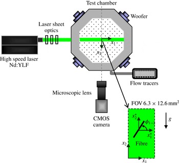
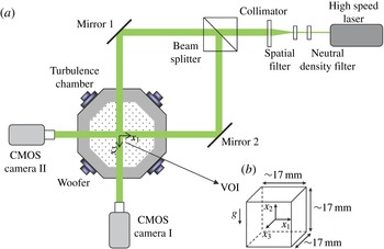
Schematic layout of the experimental facility and TR-PIV set-up (top view, not to scale);
 $g$
and associated arrow denote the direction of the gravitational acceleration.

To the best of our knowledge, the effect of fibre inertia on rotation rate has not been experimentally studied and here we use two orthogonal view, digital holographic cinematography to measure 3-D inertial fibre (
 $St=1.35$
and 2.44) velocities, orientations and rotation rates in near homogeneous, isotropic air turbulence (
 $Re_{\unicode[STIX]{x1D706}}\approx 130$
). In addition, time-resolved particle image velocimetry (TR-PIV) measurements were performed in order to characterize the unladen and fibre-laden flow field, estimate the dissipation rate and investigate fibre alignment with the flow field. The experimental set-up and data processing are discussed in §§ 2 and 3 for the TR-PIV and holography, respectively. Fibre translational velocities and associated Lagrangian autocorrelations are presented in § 4.1. Fibre orientation and alignment are discussed in § 4.2 and detailed results on fibre rotation rates are provided in § 4.3. Conclusions are summarized in § 5.
2 Experimental set-up and flow field characteristics
2.1 Experimental facility
Measurements were performed in a
 $40\times 40\times 40~\text{cm}^{3}$
turbulence chamber (Hwang & Eaton Reference Hwang and Eaton2004; Sabban & van Hout Reference Sabban and van Hout2011) having transparent acrylic windows to ensure optical access (see figure 1). Near homogeneous, isotropic air turbulence was generated by eight woofers mounted on the corners of the chamber. The woofers were forced at a randomly changing frequency (90–110 Hz) and phase in order to avoid standing waves. Input signals to the woofers were generated by an AtoD board (National Instruments) controlled by LabView software. Near-HIT in the centre of the chamber was validated by stereoscopic particle image velocimetry (SPIV) and the reader is referred to Sabban & van Hout (Reference Sabban and van Hout2011) for further details. In the following, fluctuating air velocities are denoted by
 $u_{i}$
(
 $=U_{i}-\overline{U_{i}}$
), and root-mean-square (r.m.s.) values by a prime ‘
 $\,^{\prime }\,$
’; an overbar, ‘
 $\,\bar{\;}\,$
’, denotes temporal and/or ensemble averaging and angle brackets, ‘
 $\langle \cdots \rangle$
’, indicate spatial averaging. For normalization purposes we also used,
 $u^{\prime }=(\langle u_{1}^{\prime }\rangle +\langle u_{2}^{\prime }\rangle )/2$
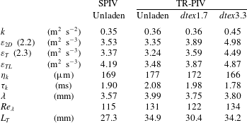
. The temporally and spatially averaged air velocities and r.m.s. values of fluctuating velocities from the SPIV pertinent to the current measurements are summarized in table 1. Statistical uncertainties in table 1 were evaluated assuming uncorrelated and normally distributed velocities (Benedict & Gould Reference Benedict and Gould1996). Under these constraints and for 95 % confidence intervals, the uncertainty of
 $\langle \overline{U_{i}}\rangle$
is
 $\pm 1.96\langle u_{i}^{\prime }\rangle /\sqrt{N}$
, where
 $N$
is the number of independent samples and the uncertainty of
 $\langle u_{i}^{\prime }\rangle$
is
 $\pm 1.96\langle u_{i}^{\prime }\rangle /\sqrt{2N}$
.
Mean and r.m.s. values of air velocities. SPIV data are taken from Sabban & van Hout (Reference Sabban and van Hout2011).

2.2 Time-resolved PIV set-up
The TR-PIV system (figure 1) comprised a CMOS camera (Photron Ultima APX,
 $512\times 1024$
pixels at 3 kHz), a high-speed laser (NewWave Pegasus, 527 nm,
 $10~\text{mJ}~\text{pulse}^{-1}$
), laser sheet optics, acquisition and data processing software (LaVision DaVis 7.4). The laser sheet (less than 1 mm thick) crossed the centre of the turbulence chamber such that the field of view (FOV) fell within the region of near-HIT (SPIV, Sabban & van Hout Reference Sabban and van Hout2011). The CMOS camera was equipped with a long working distance, microscopic lens (Infinity video lens model
 $\text{K2}/\text{S}^{\text{TM}}$
with K2 close-focus CF-2 objective) providing a FOV of
 $6.3\times 12.6~\text{mm}^{2}$
. Flow tracers generated by a smoke machine (Colt 4, tracer size 0.2–
 $0.3~\unicode[STIX]{x03BC}\text{m}$
, Glycerine BP/purified water mixture, ‘Smoke Fluid A’, Concept Engineering Limited) were introduced into the chamber after which the woofers were activated. The tracer particle size was approximately
 $0.3~\unicode[STIX]{x03BC}\text{m}$
corresponding to a Stokes number less than
 $10^{-4}$
, and resulting in a near perfect response to the highest frequency,
 $1/\unicode[STIX]{x1D70F}_{k}$
, in the present turbulent flow (Melling Reference Melling1997). Two sets of nylon fibres (material density,
 $\unicode[STIX]{x1D70C}=1.15~\text{g}~\text{cm}^{-3}$
, courtesy of Dr Ir. R. Delfos, Delft University of Technology) having the same nominal length,
 $L=0.5$
mm, but different diameters were released from the top of the chamber using a custom-made particle dispenser that consisted of a small cylindrical container. The dispenser was ‘shaken’ by a small load, eccentrically placed on the axis of an electric motor attached to the dispenser. The bottom part of the dispenser consisted of replaceable sieves with laser-drilled holes (Sabban & van Hout Reference Sabban and van Hout2011). In the present case, in order to prevent clogging, two holes with diameters of 2 mm were used.
Fibres can be characterized by their linear mass density in units of dtex (
 $=\unicode[STIX]{x03C0}\unicode[STIX]{x1D70C}D^{2}/4\times 10^{-7}$
g per 10 000 m). According to the manufacturer’s data sheet, the two used fibre sets were characterized by 1.7 and 3.3 dtex, leading to nominal diameters of
 $D=13.7~\unicode[STIX]{x03BC}\text{m}$
and
 $19.1~\unicode[STIX]{x03BC}\text{m}$
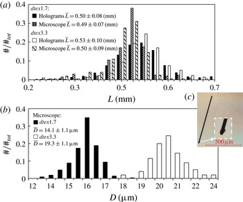
, respectively. In the following, we refer to the two fibre sets as dtex1.7 and dtex3.3 fibres. Detailed information on actual fibre length and diameter distributions (see figure 2) was obtained by analysing microscope images taken at 200
 $\times$
magnification (
 $0.022~\unicode[STIX]{x03BC}\text{m}~\text{pix}^{-1}$
, DeltaPix Invenio 2D II) using Matlab based, image processing software. Results indicate that the manufacturer’s nominal values are within 3 % of the measured mean diameters and lengths with maximum standard deviations of
 $0.07\bar{D}$
and
 $0.18\bar{L}$
, respectively. Note that the fibre diameter was measured at its centre of mass and was not affected by its edges that were slightly lopsided due to cutting (figure 2
c). In the following, nominal values are used for normalization purposes.
Measured histograms of fibre (a) length and (b) diameter; (c) fibre and magnified fibre edge imaged under a microscope.

The response time associated with the translation of randomly oriented fibres in Stokes flow depends on the aspect ratio and is given by (Bernstein & Shapiro Reference Bernstein and Shapiro1994; Zhang et al. Reference Zhang, Ahmadi, Fan and Mclaughlin2001):
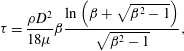 $$\begin{eqnarray}\unicode[STIX]{x1D70F}=\frac{\unicode[STIX]{x1D70C}D^{2}}{18\unicode[STIX]{x1D707}}\unicode[STIX]{x1D6FD}\frac{\ln \left(\unicode[STIX]{x1D6FD}+\sqrt{\unicode[STIX]{x1D6FD}^{2}-1}\right)}{\sqrt{\unicode[STIX]{x1D6FD}^{2}-1}},\end{eqnarray}$$
where
 $\unicode[STIX]{x1D707}$
is the air dynamic viscosity. In the present case,
 $\unicode[STIX]{x1D70F}=2.82$
ms and 5.08 ms for dtex1.7 and 3.3, respectively, and corresponding Stokes numbers are
 $St=1.35$
and 2.44.
In all cases, measurements were started at least one minute after activation of the woofers (in order to reach a statistically steady state) and just after releasing the fibres. Volume fractions were dilute,
 $\unicode[STIX]{x1D6F7}\approx 2\times 10^{-6}$
(estimated from the holography measurements described in § 3), just on the border between one- and two-way coupling (Elghobashi Reference Elghobashi1994; Poelma, Westerweel & Ooms Reference Poelma, Westerweel and Ooms2007). In total 22 data sets (10 for each dtex value and 2 unladen sets, 1.37 s per set) were acquired at 3 kHz resulting in a time separation of 0.33 ms, i.e.
 ${\sim}\unicode[STIX]{x1D70F}_{k}/6$
as will be discussed in the following.
2.3 TR-PIV data processing
Data processing consisted of distinguishing and separating fibres from flow tracers using image processing techniques (e.g. Parsheh Reference Parsheh, Brown and Aidun2005; Carlsson et al.
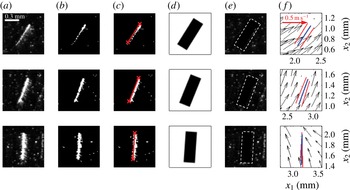
Reference Carlsson, Håkansson, Kvick, Lundell and Söderberg2011) after which images containing fibres and flow tracers were processed separately. Examples of cropped PIV images containing a single fibre as well as flow tracers depicted in figure 3(a) clearly show that the intensity signature of the fibre changes significantly due to rotation and translation in and out of the light sheet. PIV images were first converted to binary images by a user-defined threshold (figure 3
b) and fibres were subsequently detected by applying the ‘Hough’ transform that identifies line elements in binary images (Duda & Hart Reference Duda and Hart1972). Note that detected line elements could have widths up to 15 pixels due to light reflections (see figure 3
a). Gaps (5–7 pixels) between two adjacent line elements were bridged. Subsequently, the fibre centroid position and in-plane angle,
 $\unicode[STIX]{x1D719}_{1{-}2}$
(figure 1), were calculated based on a line connecting the two fibre extremities (indicated by ‘
 $\times$
’ in figure 3
c). In total, 705 and 974 fibres were detected for
 $\mathit{dtex}1.7$
and 3.3, respectively.
Procedure of fibre detection and masking of the original PIV data (
 $\unicode[STIX]{x0394}t=2$
ms between rows). (a) Cropped raw PIV image, (b) binarized image, (c) binarized image plus superimposed detected line element by Hough transform, (d) applied mask, (e) (d) multiplied by (a): dashed white rectangle denotes mask boundary, (f) resulting vector maps plus superimposed fibres. Red lines are original detected fibres while blue lines in (f) denote interpolated fibre positions.

Once detected, fibres were removed from the PIV images by placing at the centroid of each fibre, a rectangular mask of 52 by 16 pixels (approximately
 $0.6\times 0.2$
mm) rotated according to
 $\unicode[STIX]{x1D719}_{1{-}2}$
(see figure 3
d). The masked images (only containing flow tracers, figure 3
e) were pre-processed to remove any spatial non-uniformities in the light intensity and to improve the signal to noise ratio. Subsequently, velocity fields were obtained by PIV algorithms (LaVision DaVis 7.4, based on fast Fourier transforms) using multi-pass processing and decreasing interrogation window size (
 $64\times 64$
to
 $32\times 32$
pixels with 50 % overlap). The final vector spacing was
 $197~\unicode[STIX]{x03BC}\text{m}$
, i.e. comparable to
 $\unicode[STIX]{x1D702}_{k}$
(see table 2). In between passes and at the post-processing stage, outliers were removed by applying a
 $3\times 3$
median filter (Nogueira, Lecuona & Rodríguez Reference Nogueira, Lecuona and Rodríguez1997) and in the final step, a
 $3\times 3$
smoothing filter was applied. Examples of the resulting vector field in the vicinity of the fibre and superposed fibre are depicted in figure 3(f). Since each vector field was determined from two consecutive PIV images taken at times
 $t_{1}$
and
 $t_{2}$
, cubic interpolation was performed to position the fibre at
 $(t_{1}+t_{2})/2$
(blue line segment in figure 3
f). Note that in order to ensure uncorrelated vector maps, TR-PIV data were temporally averaged over vector maps spaced
 $25\unicode[STIX]{x1D70F}_{k}$
apart. At this spacing the velocity autocorrelation coefficient dropped to zero (not shown). TR-PIV ensemble and spatially averaged air velocities and r.m.s. values are summarized in table 1. Further note that convergence of first- and second-order moments was validated.
Since the FOV of the TR-PIV is very small, the mean velocities and r.m.s. velocities are compared to those obtained in the SPIV measurements performed by Sabban & van Hout (Reference Sabban and van Hout2011) in the same facility and flow conditions albeit at a much larger FOV (
 ${\sim}45\times 45~\text{mm}^{2}$
). Comparing between
 $(\langle u_{1}^{\prime }\rangle +\langle u_{2}^{\prime }\rangle )/2$
for the SPIV and unladen TR-PIV (table 1) shows that values are almost the same while
 $\langle u_{1}^{\prime }\rangle$
and
 $\langle u_{2}^{\prime }\rangle$
differ at most by 4 %. Differences between the SPIV and unladen TR-PIV results for
 $\langle \overline{U_{i}}\rangle$
and
 $\langle u_{i}^{\prime }\rangle$
are the result of the difference in FOVs, i.e. for a larger FOV (SPIV) spatial inhomogeneities are better ‘averaged out’. PDFs of normalized, fluctuating air velocities,
 $u_{i}/\langle u_{i}^{\prime }\rangle$
, for SPIV and unladen TR-PIV nearly collapsed onto normal distributions (not shown). The spatial distributions of the ratios
 $u_{1}^{\prime }/u_{2}^{\prime }$
,
 $u_{1}^{\prime }/\langle u_{1}^{\prime }\rangle$
and
 $u_{2}^{\prime }/\langle u_{2}^{\prime }\rangle$
covered the same range for TR-PIV and SPIV with maximum deviations up to 20 % of the spatially averaged values, similar to reports by Hwang & Eaton (Reference Hwang and Eaton2004) and Gopalan, Malkiel & Katz (Reference Gopalan, Malkiel and Katz2008), ensuring that near HIT was reached in the TR-PIV measurements.
Dispensing the fibres did not affect
 $\langle \overline{U_{1}}\rangle$
but
 $\langle \overline{U_{2}}\rangle$
increasingly decreased upon dispensing heavier fibres and reached
 $\langle \overline{U_{2}}\rangle =-0.44~\text{m}~\text{s}^{-1}$
for dtex3.3, only 22 % smaller than
 $\langle u_{2}^{\prime }\rangle$
. The latter observation can be attributed to secondary flow induced by the settling fibres similar as discussed by Tanaka & Eaton (Reference Tanaka and Eaton2010) for large spheres at increasing mass fraction. Furthermore, while values of
 $\langle u_{i}^{\prime }\rangle$
for dtex1.7 are similar to those obtained in the unladen case, for dtex3.3 both
 $\langle u_{1}^{\prime }\rangle$
and
 $\langle u_{2}^{\prime }\rangle$
increased 10 % and 17 %, respectively.
2.4 Dissipation rate estimate
For the present planar TR-PIV measurements and assuming isotropy, the average TKE is defined as,
 $k\equiv 3\langle \overline{(u_{1}^{2}+u_{2}^{2})}\rangle /4$
. The dissipation rate,
 $\unicode[STIX]{x1D700}\equiv 2\unicode[STIX]{x1D708}\langle \overline{s_{ij}s_{ij}}\rangle$
where
 $s_{ij}$
denotes the fluctuating rate of strain, can be estimated by (Tanaka & Eaton Reference Tanaka and Eaton2010):
 $$\begin{eqnarray}\unicode[STIX]{x1D700}_{2D}=3\unicode[STIX]{x1D708}(s_{11}^{2}+s_{22}^{2})+12\unicode[STIX]{x1D708}s_{12}^{2}.\end{eqnarray}$$
However, direct calculation of
 $\unicode[STIX]{x1D700}_{2D}$
using (2.2) is affected by a random error when the spatial measurement resolution,
 $\unicode[STIX]{x0394}x$
, is smaller than
 $\unicode[STIX]{x1D702}_{k}$
(Tanaka & Eaton Reference Tanaka and Eaton2007), and a bias error when
 $\unicode[STIX]{x0394}x>\unicode[STIX]{x1D702}_{k}$
(Lavoie et al.
Reference Lavoie, Avallone, De Gregorio, Romano and Antonia2007). In order to reduce the random error, Tanaka & Eaton (Reference Tanaka and Eaton2007) recommended calculating the dissipation rate by:
 $$\begin{eqnarray}\unicode[STIX]{x1D700}_{T}=\frac{4\unicode[STIX]{x1D700}_{2D}^{2\unicode[STIX]{x0394}x}-\unicode[STIX]{x1D700}_{2D}^{\unicode[STIX]{x0394}x}}{3},\end{eqnarray}$$
where the superscripts ‘
 $\unicode[STIX]{x0394}x$
’ and ‘
 $2\unicode[STIX]{x0394}x$
’ denote evaluating (2.2) at once and twice the spatial resolution. De Jong et al. (Reference de Jong, Cao, Woodward, Salazar, Collins and Meng2009) further suggested correcting both errors irrespective of spatial resolution constraints by first reducing the random error as proposed by Tanaka & Eaton (Reference Tanaka and Eaton2007) and subsequently applying the Lavoie et al. (Reference Lavoie, Avallone, De Gregorio, Romano and Antonia2007) correction factors that depend on
 $\unicode[STIX]{x0394}x/\unicode[STIX]{x1D702}_{k}$
. For the present measurements (
 $\unicode[STIX]{x0394}x/\unicode[STIX]{x1D702}_{k}\approx 2$
),
 $\unicode[STIX]{x1D700}_{T}$
(2.3) was divided by correction factors taken from Lavoie et al. (Reference Lavoie, Avallone, De Gregorio, Romano and Antonia2007) of 0.81 and 0.92–0.93 for the SPIV and TR-PIV measurements, respectively, in order to obtain
 $\unicode[STIX]{x1D700}_{TL}$
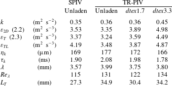
. Results are summarized in table 2, including Kolmogorov scales based on
 $\unicode[STIX]{x1D700}_{TL}$
; the Taylor microscale,
 $\unicode[STIX]{x1D706}$
; the Taylor microscale Reynolds number,
 $Re_{\unicode[STIX]{x1D706}}=\unicode[STIX]{x1D706}u^{\prime }/\unicode[STIX]{x1D708}$
; and the integral length scale
 $L_{T}=u^{\prime 3}/\unicode[STIX]{x1D700}_{TL}$
.
Summary of turbulence characteristics at the centre of the turbulence chamber.
3 Holography measurements
3.1 Digital holographic cinematography set-up
The 3-D fibre orientational and translational dynamics were measured using two orthogonal view, digital inline holographic cinematography (van Hout, Sabban & Cohen Reference van Hout, Sabban and Cohen2013), schematically depicted in figure 4. The system comprised a high-speed laser (Crystalaser,
 $10~\unicode[STIX]{x03BC}\text{J}~\text{pulse}^{-1}$
at 10 kHz), two high-speed, lensless CMOS cameras (Photron UltimaAPX,
 $1024\times 1024$
pixels at 2 kHz,
 $17~\unicode[STIX]{x03BC}\text{m}~\text{pixel}^{-1}$
), a neutral density filter and a spatial filter (aspherical focusing lens and
 $10~\unicode[STIX]{x03BC}\text{m}$
pinhole), a collimating lens having a focal length of 200 mm, a beam splitter (50–50 %, 54 mm cube, Newport) and two mirrors to direct the laser beams to the cameras. The intersection between the two collimated beams comprised the volume of interest (VOI) having an approximate size of
 $17\times 17\times 17~\text{mm}^{3}$
(see figure 4
b). Note that the TR-PIV’s FOV (see figure 1) was positioned inside the holographic VOI.
Schematic layout of (a) the experimental facility and digital holography set-up (top view, not to scale) and (b) VOI and employed coordinate system.

Holograms were recorded at the cameras’ sensor planes as a result of the interference between diffracted object beams (due to the fibres) and the undiffracted reference beam (Vikram Reference Vikram1992; Rabencov, Arca & van Hout Reference Rabencov, Arca and van Hout2014). Subsequently, the holograms were digitally reconstructed onto planes parallel but away from the sensor plane in order to determine the fibre’s orientation and position as will be discussed in § 3.2. Note that it would be difficult using the present inline set-up to measure both fibre dynamics as well as the flow field since a hologram ‘integrates’ all particle contributions (i.e. diffracted object beams) along the laser beam path. Therefore, also (tracer) particles outside the VOI will contribute to the recorded interference pattern (i.e. the hologram) leading to noisy speckle patterns that cannot be reconstructed clearly (Vikram Reference Vikram1992).
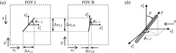
Schematic of fibre and associated coordinate systems (a) projected onto the fields of views of cameras I and II (not to scale); (b) definition of fibre polar angle and unit orientation vector in a co-moving coordinate system.

The employed coordinate systems and definitions of the fibre orientation angles are schematically depicted in figure 5 together with the FOVs of cameras I and II. Subscripts ‘I’ and ‘II’ denote camera I and II, respectively, and
 $\unicode[STIX]{x0394}x_{i}$
denote the projected, measured fibre lengths onto the corresponding
 $x_{i}$
-axes. The spatial measurement resolution was equal to the square pixel size of
 $17~\unicode[STIX]{x03BC}\text{m}$
, insufficient to resolve
 $D$
but clearly sufficient to measure
 $L$
as will be discussed in the next section. As in the TR-PIV measurements, experiments were started at least one minute after activation of the woofers (in order to reach a statistically steady state) and just after releasing the fibres. In total 8 data sets were acquired for each dtex value at an acquisition frequency,
 $f=2$
kHz, resulting in 4096 holograms (2048 for each camera) per data set. Note that
 $f\unicode[STIX]{x1D70F}_{k}^{o}=4.16$
indicating that the measurements were time resolved. The superscript ‘
 $o$
’ denotes ‘determined for the unladen TR-PIV’ (see table 2). In the following, instantaneous fibre velocities are denoted by
 $V_{i}$
, fibre fluctuating velocities by
 $v_{i}$
(
 $=V_{i}-\overline{V_{i}}$
) and
 $\unicode[STIX]{x1D719}_{1{-}2}$
and
 $\unicode[STIX]{x1D719}_{2{-}3}$
denote the fibre angles in the
 $x_{1}$
–
 $x_{2}$
and
 $x_{2}$
–
 $x_{3}$
planes, respectively (figure 5). Note that the two in-plane fibre angles were measured directly from the reconstructed holograms. The fibre polar angle,
 $\unicode[STIX]{x1D703}$
, defined in a spherical coordinate system is also depicted in figure 5(b).
3.2 Data processing
Acquired holograms were digitally reconstructed by numerically solving the Fresnel diffraction formula through convolution of the hologram intensity distribution with an impulse response function (e.g. Milgram & Li Reference Milgram and Li2002; Schnars & Jueptner Reference Schnars and Jueptner2005; van Houtet al.
Reference van Hout, Sabban and Cohen2013). We used hologram reconstruction software based on fast Fourier transform developed by Sheng, Malkiel & Katz (Reference Sheng, Malkiel and Katz2006). Due to spatial and temporal changes in the laser light intensity, reconstructed holograms suffered from poor signal-to-noise ratio that was improved by subtracting a unique background image prior to reconstruction (Rabencov et al.
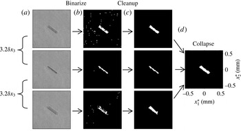
Reference Rabencov, Arca and van Hout2014). Data processing was initiated by a ‘coarse’ reconstruction of holograms acquired by one of the cameras (in this case camera I, see figures 4 and 5). ‘Coarse’ reconstruction (figure 6) means that all fibres within the VOI were detected without determining their ‘accurate’ in-focus position (in case of camera I, the position of the fibre along
 $x_{3}$
, figure 5
a). Note that determining the in-focus position is computationally highly demanding and suffers from a relatively large uncertainty inherent to single-view holography (Vikram Reference Vikram1992). Instead, the present two-view set-up relies on determining the accurate in-depth fibre position from the second camera’s FOV (figure 5). In order to detect all fibres in the VOI, the distance between ‘coarse’ reconstructions,
 $\unicode[STIX]{x1D6FF}x_{3}=1.75$
mm, was chosen carefully based on the spatial imprint of reconstructed fibres along
 $x_{3}$
(see figure 6
a). At this ‘coarse’ in-depth spatial resolution only 16 planes were reconstructed at each time instant that were subsequently binarized using a local (
 $15\times 15$
pixels), greyscale threshold value (figure 6
b) (http://www.mathworks.com/matlabcentral/fileexchange/41787-meanthresh-local-image-thresholding). The total reconstruction depth (28 mm) exceeded the depth of the intersecting VOIs of cameras I and II (see figure 4) in order to better match tracks as will be discussed in the following.
Illustration of the ‘coarse’ fibre detection scheme for camera I. (a) Cropped, background subtracted, reconstructed holograms of the same fibre at different reconstruction distances, (b) binarized images, (c) morphologically ‘cleaned’ binary images and (d) collapsed binary image.

In contrast to the TR-PIV images (see figure 3), the reconstructed holograms (figure 6
a) do not suffer from light reflections and binarized ‘blobs’ clearly show fibre outlines (figure 6
b). Therefore, most ‘blobs’ representing fibres were easily distinguished from noise based on geometrical properties such as ‘area’ (between 20 and 200 pixels) and ‘eccentricity’ exceeding 0.97 (Matlab image processing toolbox, figure 6
c). Note that as a result of applying ‘area’ and ‘eccentricity’ thresholds, tracks of fibres that came close to alignment with the
 $x_{3}$
-axis (camera I) and the
 $x_{1}$
-axis (camera II) were terminated. In practice this meant that conical volumes (in total approximately 7 % of the VOI) extending from both these axes at a polar angle of about
 $20^{\circ }$
were not sampled. Subsequently, at each time instant, binarized and morphologically cleaned, ‘coarse’ reconstructions were collapsed onto a single binary image containing the detected fibre (figure 6
d). Based on these collapsed images, fibre centroids were determined by the first moments of the ‘blob’ areas while in-plane orientation angles and fibre lengths were determined based on an ellipse having the same second moment as the ‘blob’. After determining the centroids, 2-D fibre tracks were constructed for each camera separately using a nearest neighbour algorithm (Ouellette, Xu & Bodenschatz Reference Ouellette, Xu and Bodenschatz2006; Rabencov et al.
Reference Rabencov, Arca and van Hout2014) that performed well at the present dilute volume fraction. In order to discard spurious noise, only tracks longer than 3 instances were taken into account for further processing. Furthermore, in order to reduce random measurement noise, a smoothing spline fit (Matlab’s curve fitting toolbox, smoothing parameter between 0.4 and 0.5; Green & Silverman Reference Green and Silverman1993) was applied to the fibre centroid positions and in-plane angles along each fibre track.
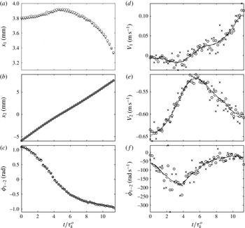
Comparison between fibre (a,b) centroid positions, (c) in-plane angles, (d,e) translational velocities and (f) in-plane rotation rates along a fibre track determined by camera I based on (
 $\times$
) in-focus reconstructions and (○) collapsed ‘coarse’ reconstructions. Symbols denote raw data while curves based on smoothed data in (d) to (f) are denoted by dashed (in-focus) and solid lines (collapsed).

In order to validate that the above described procedure provided accurate results, fibre centroid positions, translational velocities, in-plane angles and rotation rates based on in-focus and collapsed ‘coarse’ reconstructions were compared and an example for a single fibre track is shown in figure 7. Results show that besides a small bias in
 $x_{1}$
(figure 7
a, of the order of the measurement resolution, no correction was attempted), data points based on in-focus and ‘coarse’ reconstructions collapse (figure 7
a–c). Fibre translational velocities and in-plane rotation rates were calculated using a centre difference scheme while forward and backward difference schemes were applied at the start and end of the track, respectively. Higher-order difference schemes were tried but did not provide any substantial improvement. Note that in-plane and polar angle rotation rates were always assumed to change smoothly along a track (see figure 7
f). Figure 7(d–f) shows that irrespective of being based on in-focus or collapsed, ‘coarse’ reconstructions, curves based on smoothed centroid positions and fibre angles (dashed and solid lines) nearly collapse.
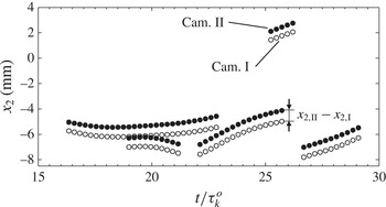
The 3-D fibre tracks were constructed by matching the in-plane tracks of both cameras based on the common
 $x_{2}$
-coordinate (figure 5). Examples displayed in figure 8 illustrate (i) a small systematic error in the common
 $x_{2}$
coordinate,
 $x_{2,II}$
–
 $x_{2,I}$
(figure 5) due to camera misalignment and (ii) the possibility of multiple fibres being present in the VOI at the same time and similar height. The first bias was easily removed and when multiple fibres were present, the pair with minimal vertical velocity difference was picked. In total 641 and 538 different 3-D fibre tracks were matched, totalling 7496 and 6619 instantaneous instances for dtex1.7 and 3.3, respectively (i.e. a mean track length of
 ${\sim}12$
instances).
Example of combining in-plane tracks from both cameras based on their common
 $x_{2}$
coordinate.

Once 3-D fibre tracks were constructed, the instantaneous fibre length and polar angle were calculated by
 $L=\sqrt{\unicode[STIX]{x0394}x_{1,I}^{2}+\unicode[STIX]{x0394}x_{2,I}^{2}+\unicode[STIX]{x0394}x_{3,II}^{2}}$
, and
 $\unicode[STIX]{x1D703}=\cos ^{-1}(\unicode[STIX]{x0394}x_{3,II}/L)$
, respectively, where
 $\unicode[STIX]{x0394}x_{2}$
was based on camera I (similar results were obtained for camera II). The fibre unit orientation vector,
 $\boldsymbol{p}$
, defined in terms of
 $\unicode[STIX]{x1D719}_{1{-}2}$
and
 $\unicode[STIX]{x1D703}$
(figure 5
b) is given by (Olson Reference Olson2001):
 $$\begin{eqnarray}\boldsymbol{p}=\left[\begin{array}{@{}c@{}}\cos \unicode[STIX]{x1D719}_{1{-}2}\sin \unicode[STIX]{x1D703}\\ \sin \unicode[STIX]{x1D719}_{1{-}2}\sin \unicode[STIX]{x1D703}\\ \cos \unicode[STIX]{x1D703}\end{array}\right]\left[\begin{array}{@{}c@{}}\hat{\boldsymbol{j}}\\ \hat{\boldsymbol{k}}\\ \hat{\boldsymbol{l}}\end{array}\right],\end{eqnarray}$$
where
 $\hat{\boldsymbol{j}},\hat{\boldsymbol{k}},\hat{\boldsymbol{l}}$
are unit vectors in the
 $x_{i}^{\ast }$
(
 $i=1,2,3$
) directions, respectively. The fibre rotation (‘tumbling’) rate is then given by:
 $$\begin{eqnarray}\dot{\boldsymbol{p}}=\dot{\unicode[STIX]{x1D719}}_{1{-}2}\sin \unicode[STIX]{x1D703}\hat{\unicode[STIX]{x1D719}}_{1{-}2}+\dot{\unicode[STIX]{x1D703}}\hat{\unicode[STIX]{x1D703}},\end{eqnarray}$$
where
 $\hat{\unicode[STIX]{x1D719}}_{1{-}2}=[-\text{sin}\,\unicode[STIX]{x1D719}_{1{-}2};\cos \unicode[STIX]{x1D719}_{1{-}2};0]$
and
 $\hat{\unicode[STIX]{x1D703}}=[\cos \unicode[STIX]{x1D719}_{1{-}2}\cos \unicode[STIX]{x1D703};\sin \unicode[STIX]{x1D719}_{1{-}2}\cos \unicode[STIX]{x1D703};-\text{sin}\,\unicode[STIX]{x1D703}]$
are the corresponding unit vectors and
 $\dot{\unicode[STIX]{x1D719}}_{1{-}2}$
and
 $\dot{\unicode[STIX]{x1D703}}$
are the fibre in-plane and polar angular velocities.
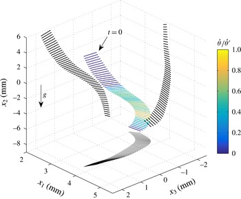
Example of a 3-D fibre track (dtex3.3), colour coded by
 $\dot{\unicode[STIX]{x1D703}}/\dot{\unicode[STIX]{x1D703}}^{\prime }$
. Black lines are the fibre projections onto planes subtended by the intersecting coordinate axes.

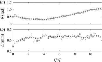
An example of a 3-D fibre track is shown in figure 9 while the associated time series of
 $\unicode[STIX]{x1D703}$
and
 $L$
are displayed in figure 10. The fibre clearly rotates in 3-D space as illustrated by its projections (solid black lines) onto the planes subtended by the intersecting coordinate axes. The fibre does not rotate ‘violently’ and
 $\dot{\unicode[STIX]{x1D703}}$
reaches a maximum equalling its r.m.s. value. Furthermore, while
 $\unicode[STIX]{x1D703}$
is expected to change along the fibre’s trajectory (figure 10
a),
 $L$
should remain constant and the scatter observed in figure 10(b) is due to noise characterized by an r.m.s. of 0.02 mm (for the smoothed data), i.e. comparable to the measurement resolution.
Time sequence of fibre (a) polar angle and (b) length along the fibre track depicted in figure 9. Based on ○ raw data and
 $\times$
smoothed data.

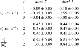
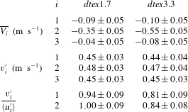
Mean and r.m.s. values of fibre centroid velocities. Uncertainties include estimates by bootstrapping clustered data (Field & Welsh Reference Field and Welsh2007) and the ‘acceleration error’ (Boillot & Prasad Reference Boillot and Prasad1996).
Histograms of fibre lengths determined from the reconstructed holograms are depicted in figure 2(a) together with those from the microscope images. The former are shifted to slightly larger
 $L$
, however, differences in mean values and standard deviations are small and do not exceed 6 % and 14 %, respectively.
4 Results
4.1 Translational fibre centroid velocities
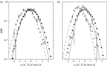
PDFs of the normalized, instantaneous (fluctuating) translational fibre centroid velocities are depicted in figure 11 together with the PDFs of the fluctuating air velocity. Corresponding mean and r.m.s. values are presented in tables 1 and 3. Mean values and uncertainties associated with fibre velocities (table 3) and rotation rates (table 4) were estimated by bootstrapping clustered data (each cluster corresponding to a different fibre track, Field & Welsh Reference Field and Welsh2007). In addition, the systematic error (‘acceleration error’, Boillot & Prasad Reference Boillot and Prasad1996) due to the finite time difference between consecutive images was estimated and when significant included. Note that convergence of mean and r.m.s. values of fibre velocities and rotation rates was validated (not shown). In order to provide an indication of the associated uncertainties, examples of representative error bars are displayed in figure 11 as well as in all following figures displaying PDFs. These error bars represent the uncertainty on the mean assuming an underlying Poisson distribution for the number of events in each bin.
PDFs of normalized, instantaneous (fluctuating) fibre centroid and flow velocities (a) dtex1.7 and (b) dtex3.3. Fibres: ○
 $i=1$
, ▵
 $i=2$
; flow: ▪
 $i=1$
. Normal distributions, fibres: (solid)
 $i=1$
, (dash-dot)
 $i=2$
; flow: (dash-dash)
 $i=1$
.

In the horizontal directions (
 $i=1,3$
), PDFs of fibre velocities collapsed and therefore only
 $v_{1}$
is presented. In the gravitational direction,
 $V_{2}/u^{\prime }$
is presented to accentuate the shift towards negative values as a result of the mean fibre settling velocity. In all cases, except for the PDF of
 $V_{2}/u^{\prime }$
(dtex3.3, figure 11
b) that is slightly skewed, PDFs are symmetric and are well described by normal distributions (based on the measured mean and standard deviation). However, for dtex3.3 (figure 11
b) fibre velocity PDFs are narrower and more peaked compared to
 $u_{1}/u^{\prime }$
. In contrast, for dtex1.7 (figure 11
a), the PDF of
 $v_{1}/u^{\prime }$
nearly collapses with that of
 $u_{1}/u^{\prime }$
. This difference is further emphasized by the ratios of fibre and air r.m.s. velocities,
 $v_{i}^{\prime }/\langle u_{i}^{\prime }\rangle$
(
 $i=1,2$
) (see table 3), that decrease from about unity for dtex1.7 to
 ${\sim}0.8$
for dtex3.3, reflecting the increased inertia of dtex3.3 fibres and resulting inability to respond to the full range of fluctuating air velocities. In the gravitational direction (
 $i=2$
), consistently slightly higher r.m.s. values are obtained than in the horizontal directions (table 3). Furthermore, the magnitude of
 $\overline{V_{2}}$
increases with increasing
 $St$
similar as
 $\langle \overline{U_{2}}\rangle$
for fibre-laden flow (see table 1). Further note that the PDFs of the relative velocities between fibre and air were symmetric around zero and could be reasonably well described by normal distributions (not shown). This is in contrast to the DNS results of Zhao, Marchioli & Andersson (Reference Zhao, Marchioli and Andersson2014) who studied the relative velocities of fibres in a turbulent channel flow and showed that PDFs of relative velocities were not normally distributed.
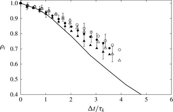
In order to characterize the effect of fibre inertia on the fibre velocity decorrelation rate, the Lagrangian autocorrelation of fluctuating, fibre centroid velocities was calculated for each direction separately by:
 $$\begin{eqnarray}\unicode[STIX]{x1D70C}_{i}(\unicode[STIX]{x0394}t)=\frac{\overline{v_{i}(t)v_{i}(t+\unicode[STIX]{x0394}t)}}{\overline{v_{i}^{2}}}.\end{eqnarray}$$
As a result of the relatively short tracks (maximum
 $7\unicode[STIX]{x1D70F}_{k}^{o}$
), the error associated with
 $\unicode[STIX]{x1D70C}_{i}$
strongly increased with increasing time separation,
 $\unicode[STIX]{x0394}t$
, and example error bars based on the analysis proposed by Snyder & Lumley (Reference Snyder and Lumley1971) are plotted in figure 12. Furthermore, since for
 $i=1$
and 3 (horizontal directions)
 $\unicode[STIX]{x1D70C}_{i}(\unicode[STIX]{x0394}t)$
collapsed, only
 $\unicode[STIX]{x1D70C}_{1}(\unicode[STIX]{x0394}t)$
and
 $\unicode[STIX]{x1D70C}_{2}(\unicode[STIX]{x0394}t)$
(gravitational direction) are plotted in figure 12 together with DNS results by Shin & Koch (Reference Shin and Koch2005) for a short inertialess fibre.
Lagrangian autocorrelation of fibre fluctuating velocities (4.1). (a) Present results (○
 $i=1$
, ▵
 $i=2$
) compared to DNS of Shin & Koch (Reference Shin and Koch2005, solid line) for a short inertialess fibre (
 $L/\unicode[STIX]{x1D702}_{k}=0.7$
); closed symbols: dtex1.7, open symbols: dtex3.3.

It can be observed that the autocorrelation curves corresponding to dtex3.3 (
 $St=2.44$
) and dtex1.7 (
 $St=1.35$
) lie above the DNS by Shin & Koch (Reference Shin and Koch2005) and decay at a slower rate, more so for the dtex3.3 fibres that have the highest Stokes number. Note that the observed decreasing decay rate is the result of the fibre’s inertia since ‘crossing trajectory’ (Yudine Reference Yudine1959; Csanady Reference Csanady1963; Reeks Reference Reeks1977) and fibre length effects (Shin & Koch Reference Shin and Koch2005) are not expected to play a role. The former is negligible when
 $V_{s}/u^{\prime }<1$
, where
 $V_{s}=\unicode[STIX]{x1D70F}g$
denotes the ‘quiescent’ fibre settling velocity while Shin & Koch (Reference Shin and Koch2005) showed that only when
 $L>7\unicode[STIX]{x1D702}_{k}$
, the autocorrelation decay rate was affected and started to decrease. Furthermore, it is observed that the autocorrelation coefficient decreases more rapidly in the direction of gravity as a result of the ‘continuity effect’ (Csanady Reference Csanady1963; Sabban & van Hout Reference Sabban and van Hout2011). The present results are in good agreement with DNS results by Squires & Eaton (Reference Squires and Eaton1991) who showed that for ‘point’ particles (
 ${<}\unicode[STIX]{x1D702}_{k}$
) in the absence of particle drift, inertia increased the autocorrelation coefficient.
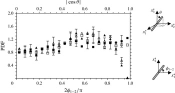
PDFs of in-plane fibre orientations, ▫
 $\unicode[STIX]{x1D719}_{1{-}2}$
(bin size 0.05); and cosine of fibre polar angles, ▵
 $|\text{cos}\,\unicode[STIX]{x1D703}|$
(bin size 0.05). Closed symbols: dtex1.7, open symbols: dtex3.3.

4.2 Fibre orientation
It is well known that fibres in isotropic turbulence align with the flow field according to the history of the ‘sampled’ velocity gradients along their trajectories (Parsa et al.
Reference Parsa, Guasto, Kishore, Ouellette, Gollub and Voth2011; Pumir & Wilkinson Reference Pumir and Wilkinson2011; Gustavsson, Einarsson & Mehlig Reference Gustavsson, Einarsson and Mehlig2014; Ni et al.
Reference Ni, Ouellette and Voth2014). However, their orientation with respect to the laboratory frame of reference is expected to be random as a result of the intense turbulence (e.g. Bernstein & Shapiro Reference Bernstein and Shapiro1994; Newsom & Bruce Reference Newsom and Bruce1998). PDFs of
 $\unicode[STIX]{x1D719}_{1{-}2}/\unicode[STIX]{x03C0}$
and the magnitude of
 $\cos \unicode[STIX]{x1D703}$
(
 $=\unicode[STIX]{x0394}x_{3,\text{II}}/L$
) displayed in figure 13 indicate that this is indeed the case and PDFs are nearly uniformly distributed for both dtex values, indicating that the fibres have random orientations. Similar results were obtained for the other projected in-plane angle,
 $\unicode[STIX]{x1D719}_{2{-}3}$
(not shown). Note that as a result of using only two perpendicular views combined with ‘area’ and ‘eccentricity’ thresholds for fibre detection (see § 3), the probability of obtaining values of
 $|\text{cos}\,\unicode[STIX]{x1D703}|$
close to one (fibre major axis aligned with
 $x_{3}$
) is zero and
 $|\text{cos}\,\unicode[STIX]{x1D703}|$
does not exceed 0.95.
However, the question remains if there is any preferential alignment of the fibres with the flow velocity and/or its derivative based quantities. Several studies in turbulent channel flows (Bernstein & Shapiro Reference Bernstein and Shapiro1994; Zhang et al.
Reference Zhang, Ahmadi, Fan and Mclaughlin2001; Marchioli et al.
Reference Marchioli, Fantoni and Soldati2010; Siewert et al.
Reference Siewert, Kunnen, Meinke and Schröder2014) found that for small
 $St$
, fibre (or ellipsoid) major axes aligned parallel to the mean flow velocity. However, for large
 $St$
, fibre major axes aligned perpendicular to the local flow direction thus maximizing the drag force (van Wachem et al.
Reference van Wachem, Zastawny, Zhao and Mallouppas2015). Since fibre alignment with the surrounding flow field is likely associated with minimizing or maximizing the net drag force (Siewert et al.
Reference Siewert, Kunnen, Meinke and Schröder2014; van Wachem et al.
Reference van Wachem, Zastawny, Zhao and Mallouppas2015), it makes sense to look at the dependence of the drag force on orientation. It is well known that the drag force on an arbitrary axisymmetric particle in steady translation (Stokes flow) along the minor and major axes is given by (Clift et al.
Reference Clift, Grace and Weber1978):
 $$\begin{eqnarray}F_{D}^{minor}=-\unicode[STIX]{x1D707}c_{1}|\boldsymbol{U}_{r}|\sin \unicode[STIX]{x1D719}_{fU_{r}},\end{eqnarray}$$
and,
 $$\begin{eqnarray}F_{D}^{major}=-\unicode[STIX]{x1D707}c_{2}|\boldsymbol{U}_{r}|\cos \unicode[STIX]{x1D719}_{fU_{r}},\end{eqnarray}$$
respectively. Here,
 $\unicode[STIX]{x1D719}_{fU_{r}}$
is the angle between the fibre’s major axis and the relative velocity vector,
 $\boldsymbol{U}_{r}=\boldsymbol{U}_{f}-\boldsymbol{V}$
(see figure 14), where
 $\boldsymbol{U}_{f}$
is the air velocity vector evaluated at the fibre’s centroid;
 $c_{1}$
and
 $c_{2}$
are the principal resistances for translation normal and parallel to the axis of symmetry, respectively. Since for a prolate spheroid (
 $\unicode[STIX]{x1D6FD}>1$
),
 $c_{1}=0.6\unicode[STIX]{x03C0}D(3+2\unicode[STIX]{x1D6FD})$
and
 $c_{2}=0.6\unicode[STIX]{x03C0}D(4+\unicode[STIX]{x1D6FD})$
, the drag will be minimal for an axisymmetric particle having its major axis aligned with
 $\boldsymbol{U}_{r}$
, i.e.
 $|\unicode[STIX]{x1D719}_{fU_{r}}|=0$
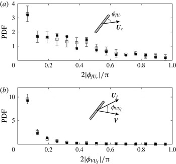
. PDFs of
 $|\unicode[STIX]{x1D719}_{fU_{r}}|/\unicode[STIX]{x03C0}$
(determined from the TR-PIV measurements) depicted in figure 14(a) for both dtex1.7 and dtex3.3, indicate a preference for the fibre’s major axis to align with
 $\boldsymbol{U}_{r}$
. In addition, PDFs of the magnitude of the angle between
 $\boldsymbol{V}$
and
 $\boldsymbol{U}_{f}$
,
 $|\unicode[STIX]{x1D719}_{VU_{f}}|/\unicode[STIX]{x03C0}$
, shown in figure 14(b), indicate a strong preference for
 $\boldsymbol{U}_{f}$
and
 $\boldsymbol{V}$
to be aligned in the same direction. This minimizes the magnitude of the relative velocity and results in the smallest possible drag force at any given fibre orientation. In combination with the fibre’s alignment with
 $\boldsymbol{U}_{r}$
(figure 14
a), this results in the minimum possible drag according to (4.2) and (4.3) (assuming Stokes flow). Note that in the present case, fibre Reynolds numbers did not exceed 15 with about 85 % of the data restricted to
 $Re<5$
(not shown).
PDFs of the in-plane angles between the instantaneous (a) fibre major axis and the relative velocity vector and (b) fibre translational velocity vector and air velocity vector sampled at the fibre’s centroid (bin sizes:
 $0.2/\unicode[STIX]{x03C0}$
).

4.3 Fibre rotation rate
Calculation of the fibre’s rotation (‘tumbling’) rate,
 $\dot{\boldsymbol{p}}$
(see (3.2)), is based on the measured polar and in-plane angle fibre rotation rates. The latter are not a linear measure of solid body rotation rate and would display very high values upon passing through
 $\unicode[STIX]{x1D703}=0^{\circ }$
(i.e. the fibre’s major axis aligning with the
 $x_{3}$
direction, see figure 5
b). However, as discussed before (§ 3), as a result of using only two orthogonal views and the adopted data processing procedure this scenario never occurred as fibre tracks were terminated when
 $\unicode[STIX]{x1D703}$
was smaller than about
 $20^{\circ }$
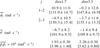
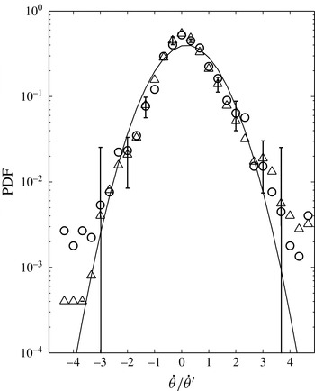
. PDFs of the normalized, in-plane and polar angle rotation rates are presented in figures 15 and 16, respectively, while mean and r.m.s. values are summarized in table 4. PDFs of normalized fibre rotation rates
 $\dot{\unicode[STIX]{x1D719}}$
and
 $\dot{\unicode[STIX]{x1D703}}$
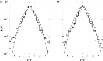
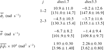
collapse for dtex1.7 and dtex3.3 and no Stokes number effects can be discerned. As expected, in-plane fibre rotation rates have the same distribution in the two measured planes (figure 15). Distributions are symmetric around zero with small mean values compared to corresponding r.m.s. values (table 4). Clearly, PDFs of both
 $\dot{\unicode[STIX]{x1D719}}/\dot{\unicode[STIX]{x1D719}}^{\prime }$
and
 $\dot{\unicode[STIX]{x1D703}}/\dot{\unicode[STIX]{x1D703}}^{\prime }$
deviate from a normal distribution indicated by the solid curve and more intense rotation events are observed in the tails of the distribution. Note that similar results were obtained for the PDFs of the rate of change of the components of the unit orientation vector (see (3.1), not shown). The present results are similar to DNS results by Marchioli & Soldati (Reference Marchioli and Soldati2013) for strongly inertial fibres (
 $\unicode[STIX]{x1D6FD}=10$
,
 $St=30$
based on the viscous time scale) but without including gravity, at the centre of a turbulent channel flow where the flow is nearly isotropic. Their PDFs of fibre angular velocity components also deviate from a normal distribution in the tails at values exceeding twice the r.m.s. Since the PDFs of fibre translational velocities were well described by a normal distribution (see figure 11), this hints at decoupling between fibre translation and rotation despite the present small
 $L/\unicode[STIX]{x1D702}_{k}$
ratio and the decoupling seen in the present results might be determined by fibre inertia.
PDFs of normalized, instantaneous in-plane fibre rotation rates for (a) dtex1.7 and (b) dtex3.3. Planes ○
 $x_{1}$
–
 $x_{2}$
, ▫
 $x_{2}$
–
 $x_{3}$
. The solid curve denotes a normal distribution.

Mean and r.m.s. values (inside square brackets) of fibre rotation rates. Values and associated uncertainties were estimated by bootstrapping clustered data (Field & Welsh Reference Field and Welsh2007).
PDFs of normalized, instantaneous fibre polar angle rotation rates. ▵ dtex1.7, ○ dtex3.3. The solid curve denotes a normal distribution.

Present results show that the r.m.s. values of dtex3.3 fibre rotation rates are consistently somewhat higher (table 4) than those of dtex1.7 that have the smallest
 $St$
. Since the rotational Stokes number is proportional to but always smaller than the translational one (see Marchioli et al.
Reference Marchioli, Zhao and Andersson2016), one would expect the opposite. A possible explanation may be that turbulence was slightly enhanced in the case of dtex3.3 fibres as indicated by the enhanced values of
 $u_{i}^{\prime }$
(see table 1). Further note that the r.m.s. values of
 $\dot{\unicode[STIX]{x1D719}}_{1{-}2}$
and
 $\dot{\unicode[STIX]{x1D719}}_{2{-}3}$
exceed those of
 $\dot{\unicode[STIX]{x1D703}}$
since in-plane angles may change even when the polar angle rotation rate is zero. Based on
 $\dot{\unicode[STIX]{x1D703}}^{\prime }$
(see table 4), it takes a fibre about 70 ms to complete a full rotation, i.e.
 ${\sim}34\unicode[STIX]{x1D70F}_{k}^{o}$
. The length scale associated with an eddy ‘turnover’ time of 70 ms is comparable to the integral length scale,
 $L_{T}$
(see table 2), indicating that fibre rotation is not dictated solely by turbulence scales ranging from the smallest Kolmogorov scales to scales of the order of the fibre length as one might expect (e.g. Shin & Koch Reference Shin and Koch2005). Instead, also the largest scales play a major role in the fibre’s rotation in agreement with Shin & Koch (Reference Shin and Koch2005) who concluded that fibre rotary motion is ‘driven’ by a wide range of scales including those larger than
 $L$
as a result of the fibre’s alignment with the local axes of strain and rotation that strongly reduced the fibre’s rotational motion.
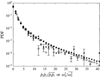
PDFs of (○) normalized, instantaneous squared fibre rotation rates and (▫) normalized, squared out-of-plane component of the vorticity. Closed symbols: dtex1.7; open symbols: dtex3.3. Literature results: ▵ experiments by Parsa et al. (Reference Parsa, Calzavarini, Toschi and Voth2012) for neutrally buoyant rods (
 $\unicode[STIX]{x1D6FD}=5$
),
 $Re_{\unicode[STIX]{x1D706}}=160$
.

Substituting the instantaneous values of
 $\unicode[STIX]{x1D719}_{1{-}2}$
,
 $\unicode[STIX]{x1D703}$
and corresponding rotation rates into (3.2), the fibre rotation rate,
 $\dot{\boldsymbol{p}}$
, was calculated. PDFs of normalized, squared instantaneous rotation (‘tumbling’) rates,
 ${\dot{p}}_{i}{\dot{p}}_{i}/\overline{{\dot{p}}_{i}{\dot{p}}_{i}}$
, are depicted in figure 17 for both dtex1.7 and 3.3 fibres and compared to Parsa et al. (Reference Parsa, Calzavarini, Toschi and Voth2012) for neutrally buoyant fibres (
 $L/\unicode[STIX]{x1D702}_{k}\approx 2.6$
,
 $\unicode[STIX]{x1D6FD}=5$
) at similar flow conditions (
 $Re_{\unicode[STIX]{x1D706}}=160$
). In addition, the out-of-plane component of the vorticity,
 $\unicode[STIX]{x1D714}_{3}=\unicode[STIX]{x2202}U_{2}/\unicode[STIX]{x2202}x_{1}-\unicode[STIX]{x2202}U_{1}/\unicode[STIX]{x2202}x_{2}$
(measured by TR-PIV), squared and normalized by
 $\overline{\unicode[STIX]{x1D714}_{3}^{2}}$
is also presented in figure 17. Note that at the present spatial resolution, the vorticity is resolved at a spatial scale comparable to the fibre length. Since fibre aspect ratio effects should be negligible (Marchioli & Soldati Reference Marchioli and Soldati2013) and mean squared rotation rates only decreased when
 $L>5\unicode[STIX]{x1D702}_{k}$
(Shin & Koch Reference Shin and Koch2005), we expect only inertia to affect the rotation rate. However, the present results for both dtex1.7 and 3.3 (
 $L=2.8\unicode[STIX]{x1D702}_{k}$
), nearly collapse with the experimental data of Parsa et al. (Reference Parsa, Calzavarini, Toschi and Voth2012) for a neutrally buoyant fibre at similar
 $L/\unicode[STIX]{x1D702}_{k}$
(
 ${\approx}2.6$
) and inertial effects cannot be discerned. This may be the result of the relatively low rotational Stokes numbers (approximately one-third of the translational Stokes numbers, see Marchioli et al.
Reference Marchioli, Zhao and Andersson2016) in the present case. Note that Parsa et al. (Reference Parsa, Calzavarini, Toschi and Voth2012) also reported DNS results at similar
 $Re_{\unicode[STIX]{x1D706}}$
that indicated a higher probability of intense rotation events compared to their experimental results. This was attributed to possible finite fibre length effects not taken into account in the DNS that might have been more substantial for intense rotation events. Their DNS results further showed that neutrally buoyant rods (
 $\unicode[STIX]{x1D6FD}=5$
) have rotation rate events exceeding those of the enstrophy. In contrast, in our case
 ${\dot{p}}_{i}{\dot{p}}_{i}/\overline{{\dot{p}}_{i}{\dot{p}}_{i}}$
fall below
 $\unicode[STIX]{x1D714}_{3}^{2}/\langle \overline{\unicode[STIX]{x1D714}_{3}^{2}}\rangle$
except for some rare events (dtex1.7) that suffer from relatively large uncertainties. Parsa et al. (Reference Parsa, Calzavarini, Toschi and Voth2012) noted that alignment variations between the fibres and the velocity gradient tensor may give rise to additional fluctuations leading to normalized, squared rotation rates exceeding those of spheres and of the enstrophy. Since in the present work only one component of the vorticity was measured, the observed discrepancy between the DNS results by Parsa et al. (Reference Parsa, Calzavarini, Toschi and Voth2012) and the present experiments might result from unequal magnitudes of different components, e.g. as a result of particle–fluid interaction (see Ferrante & Elghobashi Reference Ferrante and Elghobashi2003). However, our results do agree with experiments by Bellani et al. (Reference Bellani, Byron, Collignon, Meyer and Variano2012) who found that large, neutrally buoyant, Taylor microscale ellipsoids rotate at a slower rate than the associated, filtered (at the scale of the particle) out-of-plane vorticity.
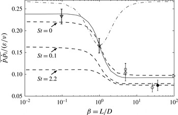
Normalized, mean squared particle rotation rate versus aspect ratio. Literature results (neutrally buoyant particles): (solid line) DNS at
 $Re_{\unicode[STIX]{x1D706}}=180$
by Parsa et al. (Reference Parsa, Calzavarini, Toschi and Voth2012); (dash dot) (4.4); DNS at ▹
 $Re_{\unicode[STIX]{x1D706}}=53.3$
,
 $L/\unicode[STIX]{x1D702}_{k}<10$
,
 $\unicode[STIX]{x1D6FD}\rightarrow \infty$
by Shin & Koch (Reference Shin and Koch2005); (dashed lines) DNS by Zhao et al. (Reference Zhao, Challabotla, Andersson and Variano2015); experiments at ▵
 $Re_{\unicode[STIX]{x1D706}}=160$
, ▫
 $Re_{\unicode[STIX]{x1D706}}=244$
by Parsa et al. (Reference Parsa, Calzavarini, Toschi and Voth2012), and ▿
 $Re_{\unicode[STIX]{x1D706}}=91$
by Marcus et al. (Reference Marcus, Parsa, Kramel, Ni and Voth2014); present results (inertial fibres): ● dtex1.7, ○ dtex3.3.

Fibre alignment and inertial effects become clear when plotting the mean squared particle rotation rate,
 $\overline{{\dot{p}}_{i}{\dot{p}}_{i}}$
, normalized by
 $(\unicode[STIX]{x1D700}/\unicode[STIX]{x1D708})$
as a function of aspect ratio (figure 18). Results are compared to experiments and DNS results by Shin & Koch (Reference Shin and Koch2005), Parsa et al. (Reference Parsa, Calzavarini, Toschi and Voth2012) and Marcus et al. (Reference Marcus, Parsa, Kramel, Ni and Voth2014) for neutrally buoyant particles at different aspect ratios. The dash-dot curve represents the mean, squared rotation rate determined from the Jeffery equation ((1.1), assuming Stokes flow, random orientation and finite aspect ratio) given by (Parsa et al.
Reference Parsa, Calzavarini, Toschi and Voth2012; Parsa Reference Parsa2013):
 $$\begin{eqnarray}\frac{\unicode[STIX]{x1D708}\overline{{\dot{p}}_{i}{\dot{p}}_{i}}}{\unicode[STIX]{x1D700}}=\frac{1}{6}+\frac{1}{10}\left(\frac{\unicode[STIX]{x1D6FD}^{2}-1}{\unicode[STIX]{x1D6FD}^{2}+1}\right).\end{eqnarray}$$
Note that for randomly oriented fibres (
 $\unicode[STIX]{x1D6FD}>1$
, dash-dot line), normalized mean squared rotation rates are much higher than for neutrally buoyant fibres that are preferentially aligned with the velocity gradient tensor (solid line, DNS by Parsa et al.
Reference Parsa, Calzavarini, Toschi and Voth2012). Experimental results for neutrally buoyant particles at different aspect ratios (Parsa et al.
Reference Parsa, Calzavarini, Toschi and Voth2012; Marcus et al.
Reference Marcus, Parsa, Kramel, Ni and Voth2014) compare well with the DNS results (solid line) that include the effect of preferential alignment. In contrast, the present measurements clearly lie below the DNS results of Parsa et al. (Reference Parsa, Calzavarini, Toschi and Voth2012) and Zhao et al. (Reference Zhao, Challabotla, Andersson and Variano2015) for inertialess particles and indicate that inertia reduces
 $\overline{{\dot{p}}_{i}{\dot{p}}_{i}}/(\unicode[STIX]{x1D700}/\unicode[STIX]{x1D708})$
, more so for dtex3.3 fibres (
 $St=2.44$
) than for dtex1.7 (
 $St=1.35$
). The present results are in good agreement with the recent DNS by Zhao et al. (Reference Zhao, Challabotla, Andersson and Variano2015) who studied the effect of fibre inertia in a turbulent channel flow and showed that fibre rotation rates decreased with increasing
 $St$
at the centre of a turbulent channel where the flow was nearly isotropic.
5 Summary and conclusions
The present study was aimed at quantifying inertial effects on 3-D fibre orientation, translational velocities and angular rotation rates. Measurements were performed in nearly homogeneous, isotropic air turbulence that was generated at the centre of a cubic chamber (
 $40\times 40\times 40~\text{cm}^{3}$
) by eight synthetic jets originating from the chamber’s corners. Two different sets of rigid, heavy (inertial) nylon fibres having the same length,
 $L=0.5$
mm, but different diameters,
 $D=13.7~\unicode[STIX]{x03BC}\text{m}$
(dtex1.7,
 $\unicode[STIX]{x1D6FD}=36.5$
) and
 $19.1~\unicode[STIX]{x03BC}\text{m}$
(dtex3.3,
 $\unicode[STIX]{x1D6FD}=26.2$
), were released at dilute conditions from the top of the chamber by a custom-made dispenser. The dtex1.7 and dtex3.3 fibres were characterized by
 $St=1.35$
and 2.44, respectively. The fibres were imaged from two orthogonal directions by digital holographic cinematography at an acquisition rate approximately five times higher than the Kolmogorov frequency. The Taylor microscale Reynolds number was
 $Re_{\unicode[STIX]{x1D706}}\approx 130$
, and the spatial resolution
 $17~\unicode[STIX]{x03BC}\text{m}~\text{pix}^{-1}$
. The volume of interest, i.e. the intersection of the two orthogonal views, was approximately
 $17\times 17\times 17~\text{mm}^{3}$
located at the centre of the turbulence chamber. In addition to the holography, planar time-resolved PIV measurements were performed in order to characterize the flow characteristics, estimate the TKE dissipation rate and study fibre alignment with the flow. Using a long working distance microscopic lens, a FOV of
 $6.3\times 12.6~\text{mm}^{2}$
was obtained leading to a spatial resolution comparable to the Kolmogorov length scale.
Comparing the PDFs of fluctuating air velocities (that were normally distributed) to those of the fluctuating fibre velocities, revealed that the dtex3.3 fibres (
 $St=2.44$
) were unable to sample the full range of air fluctuating velocities and their PDFs were narrower than those of the air. In contrast, PDFs of dtex1.7 fluctuating fibre velocities nearly collapsed with those of the air. This was further emphasized by the ratios between the r.m.s. values of fluctuating fibre and air velocities that were approximately unity for dtex1.7 fibres and reduced to approximately 0.8 for dtex3.3 fibres. A comparison between the Lagrangian autocorrelation of fibre translational velocities of non-inertial and the present inertial fibres showed that increasing inertia (indicated by increasing
 $St$
) decreased the decrease rate of the velocity autocorrelation (in the absence of the ‘crossing’ trajectory effect and fibre length effects) similar as for spherical particles. Furthermore, in the direction of gravity, the autocorrelation decay rate decreased faster than in the horizontal directions due to the ‘continuity’ effect (Yudine Reference Yudine1959).
As a result of the intense turbulence generated in the turbulence chamber, fibre orientations in the camera’s frame of reference were uniformly distributed across all possible angles. However, it is well known that fibres preferentially align with the flow and this was further investigated by analysing the TR-PIV measurements that resolved both the instantaneous flow and fibre orientation albeit in a plane. In particular, it was found that the fibre’s translational centroid velocity vector shows a strong preference to align with that of the flow (interpolated onto the fibre’s centroid) while its major axis also preferentially aligns with the relative velocity vector. The overall result of this alignment is that the drag force acting on the fibre is minimized.
PDFs of fibre in-plane and polar angle rotation rates based on the holography measurements and normalized by their respective r.m.s. values, deviated from a normal distribution but collapsed for both dtex values. Furthermore, results indicated the occurrence of extreme rotation rate events in the tails of the distribution similar as those obtained in the DNS by Marchioli & Soldati (Reference Marchioli and Soldati2013) for fibres at the centre of a turbulent channel where the flow was nearly isotropic. In addition, PDFs of the squared instantaneous, fibre rotation (‘tumbling’) rates normalized by their respective r.m.s. values also collapsed for both dtex values as well as with the measurements by Parsa et al. (Reference Parsa, Calzavarini, Toschi and Voth2012) for neutrally buoyant fibres. However, in contrast with the latter results that showed that extreme fibre rotation events may exceed those of the flow enstrophy our results indicate that normalized squared fibre rotation rates are lower than the normalized, squared out-of-plane component of the vorticity.
The effect of fibre inertia and alignment was most clearly observed upon plotting the normalized mean squared rotation rate,
 $\overline{{\dot{p}}_{i}{\dot{p}}_{i}}/(\unicode[STIX]{x1D700}/\unicode[STIX]{x1D708})$
, as a function of aspect ratio together with DNS results and some experimental data points. Results clearly indicated that in the present measurements, the fibres were preferentially aligned with the flow as indicated by the strongly reduced rotation rates in comparison to randomly oriented fibres. In addition, the effect of inertia was to further reduce
 $\overline{{\dot{p}}_{i}{\dot{p}}_{i}}/(\unicode[STIX]{x1D700}/\unicode[STIX]{x1D708})$
. The present results were in excellent agreement with recent DNS by Zhao et al. (Reference Zhao, Challabotla, Andersson and Variano2015) that considered the effect of inertia on fibre rotation rates at the centre of a turbulent channel flow. To the best of our knowledge, these are the first experiments that quantified the effect of inertia on the normalized, mean squared fibre rotation rate in near HIT.
Acknowledgements
This work was supported in part by the Edmund J. Safra Philanthropic Foundation, the Wolfson Family Charitable Trust, the Technion Fund for Promotion of Research and the Israel Science Foundation under grant no. 915/10. We also acknowledge the support of EU COST Action FP1005.