2 Governing equations

In this section, we summarize the governing equations of the NGF model for dense, steady granular flow (Kamrin & Koval Reference Kamrin and Koval2012; Henann & Kamrin Reference Henann and Kamrin2013, Reference Henann and Kamrin2014b ; Liu & Henann Reference Liu and Henann2017). Like the LI rheology, the NGF model is a continuum approach for modelling steady, dense flows of quasi-monodisperse systems of dry, stiff grains. Throughout this paper, we use standard component notation, which supposes an underlying set of Cartesian basis vectors $\{\boldsymbol{e}_{i}|i=1,2,3\}$ , and in which the components of vectors, $\boldsymbol{v}$ , and tensors, $\unicode[STIX]{x1D748}$ , are denoted by $v_{i}$ and $\unicode[STIX]{x1D70E}_{ij}$ , respectively. The Einstein summation convention is employed, and the Kronecker delta, $\unicode[STIX]{x1D6FF}_{ij}$ , is utilized to denote the components of the identity tensor.

The kinematics of flow are described by the velocity field $v_{i}(\boldsymbol{x},t)$ , where $x_{i}$ denotes the spatial coordinate and $t$ time. The velocity gradient, stretching and spin tensors are then

(2.1a-c ) $$\begin{eqnarray}\displaystyle \unicode[STIX]{x1D613}_{ij}=\frac{\unicode[STIX]{x2202}v_{i}}{\unicode[STIX]{x2202}x_{j}},\quad \unicode[STIX]{x1D60B}_{ij}=\frac{1}{2}\left(\frac{\unicode[STIX]{x2202}v_{i}}{\unicode[STIX]{x2202}x_{j}}+\frac{\unicode[STIX]{x2202}v_{j}}{\unicode[STIX]{x2202}x_{i}}\right),\quad \unicode[STIX]{x1D61E}_{ij}=\frac{1}{2}\left(\frac{\unicode[STIX]{x2202}v_{i}}{\unicode[STIX]{x2202}x_{j}}-\frac{\unicode[STIX]{x2202}v_{j}}{\unicode[STIX]{x2202}x_{i}}\right), & & \displaystyle\end{eqnarray}$$

respectively. We make the common approximation that steady, well-developed flow proceeds at constant volume (Jop et al. Reference Jop, Forterre and Pouliquen2006; Rycroft, Kamrin & Bazant Reference Rycroft, Kamrin and Bazant2009; Kamrin Reference Kamrin2010), so that the velocity field is divergence-free, $\unicode[STIX]{x2202}v_{j}/\unicode[STIX]{x2202}x_{j}=0$ , and the velocity gradient and stretching tensors are deviatoric, i.e. $\unicode[STIX]{x1D613}_{jj}=\unicode[STIX]{x1D60B}_{jj}=0$ . Finally, we define the equivalent shear strain rate as $\dot{\unicode[STIX]{x1D6FE}}=(2\unicode[STIX]{x1D60B}_{ij}\unicode[STIX]{x1D60B}_{ij})^{1/2}$ and the symmetric and deviatoric direction of flow as $\unicode[STIX]{x1D615}_{ij}=\sqrt{2}\unicode[STIX]{x1D60B}_{ij}/\dot{\unicode[STIX]{x1D6FE}}$ . Note that the flow direction tensor is defined to be a unit tensor – i.e. $\unicode[STIX]{x1D615}_{ij}\unicode[STIX]{x1D615}_{ij}=1$ – and differs by a factor of $\sqrt{2}$ from that used by Barker et al. (Reference Barker, Schaeffer, Bohorquez and Gray2015).

The symmetric Cauchy stress tensor and stress deviator are denoted as $\unicode[STIX]{x1D70E}_{ij}=\unicode[STIX]{x1D70E}_{ji}$ and $\unicode[STIX]{x1D70E}_{ij}^{\prime }=\unicode[STIX]{x1D70E}_{ij}-(1/3)(\unicode[STIX]{x1D70E}_{kk})\unicode[STIX]{x1D6FF}_{ij}$ . Then, we define the equivalent shear stress, the pressure and the Drucker–Prager stress ratio as $\unicode[STIX]{x1D70F}=(\unicode[STIX]{x1D70E}_{ij}^{\prime }\unicode[STIX]{x1D70E}_{ij}^{\prime }/2)^{1/2}$ , $P=-\unicode[STIX]{x1D70E}_{kk}/3$ and $\unicode[STIX]{x1D707}=\unicode[STIX]{x1D70F}/P$ , respectively, and emphasize that these quantities represent stress-tensor invariants. The Cauchy stress must satisfy the standard equations of motion

(2.2) $$\begin{eqnarray}\displaystyle \unicode[STIX]{x1D719}\unicode[STIX]{x1D70C}_{s}\left(\frac{\unicode[STIX]{x2202}v_{i}}{\unicode[STIX]{x2202}t}+v_{j}\frac{\unicode[STIX]{x2202}v_{i}}{\unicode[STIX]{x2202}x_{j}}\right)=\frac{\unicode[STIX]{x2202}\unicode[STIX]{x1D70E}_{ij}}{\unicode[STIX]{x2202}x_{j}}+b_{i}, & & \displaystyle\end{eqnarray}$$

where $\unicode[STIX]{x1D719}$ is the solid volume fraction and $b_{i}$ is the non-inertial body force per unit volume (typically gravitational). For the purposes of the present work, we consider situations in which body forces are absent, so that $b_{i}=0_{i}$ in what follows.

In a local constitutive approach, the governing equations are closed through a constitutive equation relating the stress tensor $\unicode[STIX]{x1D70E}_{ij}$ to the stretching tensor $\unicode[STIX]{x1D60B}_{ij}$ in a manner consistent with (1.1) (e.g. Jop et al. Reference Jop, Forterre and Pouliquen2006). Instead, in our non-local constitutive approach, an additional positive, scalar state variable, called the granular fluidity, is introduced and denoted as $g$ . (Due to its reliance on an additional field quantity, the NGF model bears a resemblance to so-called ‘implicit’ gradient theories in the plasticity literature (e.g. Engelen, Geers & Baaijens Reference Engelen, Geers and Baaijens2003).) The granular fluidity, $g$ , is a kinematic state variable that characterizes microscopic fluctuations in a flowing granular medium. More precisely, Zhang & Kamrin (Reference Zhang and Kamrin2017) and Bhateja & Khakhar (Reference Bhateja and Khakhar2018) have established that the granular fluidity has a kinematic definition that holds across a variety of inhomogeneous flow configurations for both two- and three-dimensional dense granular systems and is given through the relation $g=(\unicode[STIX]{x1D6FF}v/d)F(\unicode[STIX]{x1D719})$ , where $\unicode[STIX]{x1D6FF}v$ is the velocity fluctuation, $\unicode[STIX]{x1D719}$ is the solid volume fraction, $d$ is the grain size and $F(\unicode[STIX]{x1D719})$ is a function of only $\unicode[STIX]{x1D719}$ . Then, in the NGF model, the stress tensor, stretching tensor and granular fluidity are related through two phenomenological constitutive relations: (1) the flow rule and (2) the non-local rheology.

First, regarding the flow rule, assuming that the strain-rate tensor and stress deviator are co-directional – i.e. $\unicode[STIX]{x1D615}_{ij}=\sqrt{2}\unicode[STIX]{x1D60B}_{ij}/\dot{\unicode[STIX]{x1D6FE}}=\unicode[STIX]{x1D70E}_{ij}^{\prime }/\sqrt{2}\unicode[STIX]{x1D70F}$ (Jop et al. Reference Jop, Forterre and Pouliquen2006; Rycroft et al. Reference Rycroft, Kamrin and Bazant2009; Kamrin Reference Kamrin2010) – the stress tensor, $\unicode[STIX]{x1D70E}_{ij}$ , the stretching tensor, $\unicode[STIX]{x1D60B}_{ij}$ , and the granular fluidity, $g$ , are taken to be related through

(2.3) $$\begin{eqnarray}\displaystyle \unicode[STIX]{x1D70E}_{ij}=-P\unicode[STIX]{x1D6FF}_{ij}+2\frac{P}{g}\unicode[STIX]{x1D60B}_{ij}. & & \displaystyle\end{eqnarray}$$

We note that co-directionality is an approximation, and slight deviations from co-directionality – such as normal stress differences – have been observed in discrete-element simulations (e.g. Weinhart et al. Reference Weinhart, Hartkamp, Thornton and Luding2013). However, co-directionality remains a useful simplifying assumption and enables a reasonably good description of experimental data. Taking the inner product of the tensorial constitutive relation (2.3) with $\unicode[STIX]{x1D615}_{ij}$ and rearranging gives the following scalar form of the flow rule, relating the equivalent shear strain rate, the granular fluidity and the Drucker–Prager stress ratio:

(2.4) $$\begin{eqnarray}\displaystyle \dot{\unicode[STIX]{x1D6FE}}=g\unicode[STIX]{x1D707}, & & \displaystyle\end{eqnarray}$$

which makes clear the constitutive role of $g$ as a fluidity-like quantity that relates the stress ratio $\unicode[STIX]{x1D707}$ to the shear strain rate $\dot{\unicode[STIX]{x1D6FE}}$ .

Second, regarding the non-local rheology, with the introduction of the granular fluidity field, $g$ , an additional governing equation is required to relate the fluidity field to the stress field and close the system of equations. In the NGF model, the granular fluidity, $g$ , is governed by the following partial differential equation (PDE):

(2.5) $$\begin{eqnarray}\displaystyle g=g_{loc}(\unicode[STIX]{x1D707},P)+\unicode[STIX]{x1D709}^{2}(\unicode[STIX]{x1D707})\frac{\unicode[STIX]{x2202}^{2}g}{\unicode[STIX]{x2202}x_{j}\unicode[STIX]{x2202}x_{j}}, & & \displaystyle\end{eqnarray}$$

where

(2.6) $$\begin{eqnarray}\displaystyle g_{loc}(\unicode[STIX]{x1D707},P)=\sqrt{\frac{P}{d^{2}\unicode[STIX]{x1D70C}_{s}}}\frac{I_{loc}(\unicode[STIX]{x1D707})}{\unicode[STIX]{x1D707}} & & \displaystyle\end{eqnarray}$$

is the local fluidity function, given through the stress invariants $\unicode[STIX]{x1D707}$ and $P$ ;

(2.7) $$\begin{eqnarray}\displaystyle I_{loc}(\unicode[STIX]{x1D707})=\left\{\begin{array}{@{}ll@{}}\unicode[STIX]{x1D707}_{loc}^{-1}(\unicode[STIX]{x1D707}) & \text{if }\unicode[STIX]{x1D707}>\unicode[STIX]{x1D707}_{s}\\ 0 & \text{if }\unicode[STIX]{x1D707}\leqslant \unicode[STIX]{x1D707}_{s}\end{array}\right. & & \displaystyle\end{eqnarray}$$

is the inverted form of the $\unicode[STIX]{x1D707}_{loc}(I)$ function, given through the stress ratio, $\unicode[STIX]{x1D707}$ ; and $\unicode[STIX]{x1D709}(\unicode[STIX]{x1D707})$ is a stress-dependent length scale called the cooperativity length – to be discussed further momentarily. Note that in the absence of stress or flow gradients ( $\unicode[STIX]{x2202}^{2}g/\unicode[STIX]{x2202}x_{j}\unicode[STIX]{x2202}x_{j}=0$ ), the PDE (2.5) simply reduces to the algebraic expression $g=g_{loc}(\unicode[STIX]{x1D707},P)$ , which when combined with (2.3) yields the tensorial form of the LI rheology of Jop et al. (Reference Jop, Forterre and Pouliquen2006). However, for inhomogeneous flow, the presence of the Laplacian term gives rise to non-local effects – with predictions of the NGF model being size-dependent through the cooperativity length, $\unicode[STIX]{x1D709}$ – and enables the NGF model to capture the loss of local constitutive uniqueness between $\unicode[STIX]{x1D707}$ and $I$ observed in experiments and discrete-element method simulations of dense granular flow (e.g. Koval et al. Reference Koval, Roux, Corfdir and Chevoir2009).

We note that the non-local rheology (2.5) represents a simplified form of the NGF model, specialized for quasi-steady flow situations. The primitive form of the NGF model utilizes a Ginzberg–Landau-type dynamical PDE in place of (2.5), in which $g$ operates as a non-local order parameter. The steady-state form (2.5) then arises as the approximate solution of the stable, quasi-steady behaviour of $g$ in the dynamical PDE – valid as long as $g$ remains sufficiently close to the local fluidity (2.6). In the present work, we focus attention on the mathematical properties of the system of equations involving the steady-state form (2.5) and do not discuss the dynamical form of the NGF model in detail here, instead referring interested readers to several of our previous works for further discussion (Henann & Kamrin Reference Henann and Kamrin2014b ; Kamrin & Henann Reference Kamrin and Henann2015; Liu & Henann Reference Liu and Henann2017). However, it is important to point out that the precise functional form of the stress-dependent cooperativity length, $\unicode[STIX]{x1D709}(\unicode[STIX]{x1D707})$ , emerges from the process of reducing the dynamical form of the NGF model to the steady-state form (2.5) and is connected to the choice of the $\unicode[STIX]{x1D707}_{loc}(I)$ function. For the Bingham-like functional form (1.2) and the functional form of Jop et al. (Reference Jop, Forterre and Pouliquen2005) (1.3), the corresponding functional forms for the cooperativity length are

(2.8a,b ) $$\begin{eqnarray}\displaystyle \unicode[STIX]{x1D709}(\unicode[STIX]{x1D707})=\frac{Ad}{\sqrt{|\unicode[STIX]{x1D707}-\unicode[STIX]{x1D707}_{s}|}}\quad \text{and}\quad \unicode[STIX]{x1D709}(\unicode[STIX]{x1D707})=Ad\sqrt{\frac{(\unicode[STIX]{x1D707}_{2}-\unicode[STIX]{x1D707})}{(\unicode[STIX]{x1D707}_{2}-\unicode[STIX]{x1D707}_{s})|\unicode[STIX]{x1D707}-\unicode[STIX]{x1D707}_{s}|}}, & & \displaystyle\end{eqnarray}$$

respectively. In both cases, the cooperativity length is directly proportional to the grain size, $d$ , and the parameter $A$ is a dimensionless material constant, referred to as the non-local amplitude, which quantifies the spatial extent of cooperative effects. We note that the non-local amplitude, $A$ , is the only new material parameter introduced in the NGF model beyond the parameters appearing in the LI rheology – i.e. $\{\unicode[STIX]{x1D707}_{s},b\}$ for the Bingham-like form (1.2) and $\{\unicode[STIX]{x1D707}_{s},\unicode[STIX]{x1D707}_{2},b\}$ the form of Jop et al. (Reference Jop, Forterre and Pouliquen2005) (1.3). For $\unicode[STIX]{x1D707}$ in the neighbourhood of $\unicode[STIX]{x1D707}_{s}$ , both expressions for the cooperativity length behave similarly, diverging as $\unicode[STIX]{x1D707}$ approaches $\unicode[STIX]{x1D707}_{s}$ . The major difference between the two expressions is that for the case in which $\unicode[STIX]{x1D707}_{loc}(I)$ possesses an upper limiting value $\unicode[STIX]{x1D707}_{2}$ (1.3), the cooperativity length goes to zero as $\unicode[STIX]{x1D707}$ approaches $\unicode[STIX]{x1D707}_{2}$ .

Finally, we summarize the field equations governing the velocity field, the pressure field and the granular fluidity field in a form appropriate for the linear stability analysis of § 3. First, incompressibility requires that the velocity field be divergence-free:

(2.9) $$\begin{eqnarray}\displaystyle \frac{\unicode[STIX]{x2202}v_{j}}{\unicode[STIX]{x2202}x_{j}}=0. & & \displaystyle\end{eqnarray}$$

Second, substituting the tensorial form of the flow rule (2.3) into (2.2) allows the equations of motion to be written explicitly in terms of the velocity, pressure and fluidity fields as

(2.10) $$\begin{eqnarray}\displaystyle \unicode[STIX]{x1D719}\unicode[STIX]{x1D70C}_{s}\left(\frac{\unicode[STIX]{x2202}v_{i}}{\unicode[STIX]{x2202}t}+v_{j}\frac{\unicode[STIX]{x2202}v_{i}}{\unicode[STIX]{x2202}x_{j}}\right)=\left(-\unicode[STIX]{x1D6FF}_{ij}+\frac{2}{g}\unicode[STIX]{x1D60B}_{ij}\right)\frac{\unicode[STIX]{x2202}P}{\unicode[STIX]{x2202}x_{j}}+\frac{P}{g}\frac{\unicode[STIX]{x2202}^{2}v_{i}}{\unicode[STIX]{x2202}x_{j}\unicode[STIX]{x2202}x_{j}}-2\frac{P}{g^{2}}\unicode[STIX]{x1D60B}_{ij}\frac{\unicode[STIX]{x2202}g}{\unicode[STIX]{x2202}x_{j}}, & & \displaystyle\end{eqnarray}$$

where body forces such as gravity have been omitted. Finally, the scalar form of the flow rule (2.4) may be used to express the non-local rheology (2.5) as

(2.11) $$\begin{eqnarray}\displaystyle g=g_{loc}(\dot{\unicode[STIX]{x1D6FE}}/g,P)+\unicode[STIX]{x1D709}^{2}(\dot{\unicode[STIX]{x1D6FE}}/g)\frac{\unicode[STIX]{x2202}^{2}g}{\unicode[STIX]{x2202}x_{j}\unicode[STIX]{x2202}x_{j}}, & & \displaystyle\end{eqnarray}$$

with the local fluidity and cooperativity length functions, $g_{loc}(\dot{\unicode[STIX]{x1D6FE}}/g,P)$ and $\unicode[STIX]{x1D709}(\dot{\unicode[STIX]{x1D6FE}}/g)$ , given through (2.6), (2.7) and (2.8). Hence, the governing equations consist of incompressibility (2.9), the equations of motion (2.10) and the non-local rheology (2.11) and constitute a closed system of equations for the velocity field, $v_{i}$ , the pressure field, $P$ , and the fluidity field, $g$ .

3 Linear stability of the NGF model

In this section, we present our linear stability analysis of the NGF model. We consider a base state that corresponds to steady, homogeneous, constant-volume flow in an infinite domain and denote the base-state fields, $v_{i}^{0}$ , $P^{0}$ and $g^{0}$ , with a superscript 0. Accordingly, we take $v_{i}^{0}(\boldsymbol{x})$ to vary linearly in space as $v_{i}^{0}(\boldsymbol{x})=\unicode[STIX]{x1D613}_{ij}^{0}x_{j}$ , where $\unicode[STIX]{x1D613}_{ij}^{0}$ is the spatially constant and deviatoric base-state velocity gradient. Therefore, the base-state flow satisfies incompressibility, i.e. $\unicode[STIX]{x2202}v_{j}^{0}/\unicode[STIX]{x2202}x_{j}=\unicode[STIX]{x1D613}_{jj}^{0}=0$ , and $\unicode[STIX]{x1D60B}_{ij}^{0}=(1/2)(\unicode[STIX]{x1D613}_{ij}^{0}+\unicode[STIX]{x1D613}_{ji}^{0})$ is the spatially constant and deviatoric base-state stretching tensor. The base-state pressure is also taken to be spatially constant, and we define the base-state equivalent shear strain rate, direction of flow and inertial number as $\dot{\unicode[STIX]{x1D6FE}}^{0}=(2\unicode[STIX]{x1D60B}_{ij}^{0}\unicode[STIX]{x1D60B}_{ij}^{0})^{1/2}$ , $\unicode[STIX]{x1D615}_{ij}^{0}=\sqrt{2}\unicode[STIX]{x1D60B}_{ij}^{0}/\dot{\unicode[STIX]{x1D6FE}}^{0}$ and $I^{0}=\dot{\unicode[STIX]{x1D6FE}}^{0}\sqrt{d^{2}\unicode[STIX]{x1D70C}_{s}/P^{0}}$ , respectively. Regarding the base-state fluidity, for homogeneous flow, we take $g^{0}$ to be spatially constant, and in order to be consistent with (2.11), $g^{0}$ is given implicitly through $g^{0}=g_{loc}(\dot{\unicode[STIX]{x1D6FE}}^{0}/g^{0},P^{0})$ , which due to (2.6) and (2.7) implies that the base-state fluidity is given explicitly through the $\unicode[STIX]{x1D707}_{loc}(I)$ function as $g^{0}=\dot{\unicode[STIX]{x1D6FE}}^{0}/\unicode[STIX]{x1D707}_{loc}(I^{0})$ .

3.1 Linearized governing equations

We then consider perturbed velocity, pressure and fluidity fields of the form

(3.1a-c ) $$\begin{eqnarray}\displaystyle v_{i}=v_{i}^{0}(\boldsymbol{x})+\hat{v}_{i}(\boldsymbol{x},t),\quad P=P^{0}+\hat{P}(\boldsymbol{x},t)\quad \text{and}\quad g=g^{0}+{\hat{g}}(\boldsymbol{x},t), & & \displaystyle\end{eqnarray}$$

where $\hat{v}_{i}$ , $\hat{P}$ and ${\hat{g}}$ represent small perturbations of the base-state fields. First, the incompressibility constraint requires that

(3.2) $$\begin{eqnarray}\displaystyle \frac{\unicode[STIX]{x2202}\hat{v}_{j}}{\unicode[STIX]{x2202}x_{j}}=0. & & \displaystyle\end{eqnarray}$$

Second, linearizing the equations of motion (2.10), we obtain

(3.3) $$\begin{eqnarray}\displaystyle \unicode[STIX]{x1D719}\unicode[STIX]{x1D70C}_{s}\left(\frac{\unicode[STIX]{x2202}\hat{v}_{i}}{\unicode[STIX]{x2202}t}+v_{j}^{0}\frac{\unicode[STIX]{x2202}\hat{v}_{i}}{\unicode[STIX]{x2202}x_{j}}+\unicode[STIX]{x1D613}_{ij}^{0}\hat{v}_{j}\right)=\left(-\unicode[STIX]{x1D6FF}_{ij}+\frac{2}{g^{0}}\unicode[STIX]{x1D60B}_{ij}^{0}\right)\frac{\unicode[STIX]{x2202}\hat{P}}{\unicode[STIX]{x2202}x_{j}}+\frac{P^{0}}{g^{0}}\frac{\unicode[STIX]{x2202}^{2}\hat{v}_{i}}{\unicode[STIX]{x2202}x_{j}\unicode[STIX]{x2202}x_{j}}-2\frac{P^{0}}{{g^{0}}^{2}}\unicode[STIX]{x1D60B}_{ij}^{0}\frac{\unicode[STIX]{x2202}{\hat{g}}}{\unicode[STIX]{x2202}x_{j}}, & & \displaystyle\end{eqnarray}$$

where we have used the fact that the base state is homogeneous – i.e. $\unicode[STIX]{x2202}P^{0}/\unicode[STIX]{x2202}x_{j}$ , $\unicode[STIX]{x2202}^{2}v_{i}^{0}/\unicode[STIX]{x2202}x_{j}\unicode[STIX]{x2202}x_{j}$ and $\unicode[STIX]{x2202}g^{0}/\unicode[STIX]{x2202}x_{j}$ vanish. The second and third terms on the left-hand side of (3.3) arise due to convection, and as pointed out by Goddard & Lee (Reference Goddard and Lee2017), these terms can play a role in the linear stability analysis and lead to asymptotic stabilization of non-convective instabilities. However, our primary interest is in examining the ellipticity of the quasi-static field equations of the NGF model, so we neglect these terms and focus on the non-convective case. For completeness, we discuss the issue of convection and its effect on linear stability in appendix A. Dropping the convective terms and substituting the base-state fluidity, $g^{0}=\dot{\unicode[STIX]{x1D6FE}}^{0}/\unicode[STIX]{x1D707}_{loc}(I^{0})$ , into (3.3) yields the following linearized equations of motion:

(3.4) $$\begin{eqnarray}\displaystyle \unicode[STIX]{x1D719}\unicode[STIX]{x1D70C}_{s}\frac{\unicode[STIX]{x2202}\hat{v}_{i}}{\unicode[STIX]{x2202}t}=(-\unicode[STIX]{x1D6FF}_{ij}+\sqrt{2}\unicode[STIX]{x1D707}_{loc}(I^{0})\unicode[STIX]{x1D615}_{ij}^{0})\frac{\unicode[STIX]{x2202}\hat{P}}{\unicode[STIX]{x2202}x_{j}}+\frac{\unicode[STIX]{x1D707}_{loc}(I^{0})P^{0}}{\dot{\unicode[STIX]{x1D6FE}}^{0}}\frac{\unicode[STIX]{x2202}^{2}\hat{v}_{i}}{\unicode[STIX]{x2202}x_{j}\unicode[STIX]{x2202}x_{j}}-\sqrt{2}\frac{\unicode[STIX]{x1D707}_{loc}^{2}(I^{0})P^{0}}{\dot{\unicode[STIX]{x1D6FE}}^{0}}\unicode[STIX]{x1D615}_{ij}^{0}\frac{\unicode[STIX]{x2202}{\hat{g}}}{\unicode[STIX]{x2202}x_{j}}.\quad & & \displaystyle\end{eqnarray}$$

Finally, the linearization of the non-local rheology (2.11) is described in appendix B and results in the following expression relating the perturbed pressure, velocity and fluidity fields:

(3.5) $$\begin{eqnarray}\displaystyle \frac{1}{2\unicode[STIX]{x1D702}^{0}}\hat{P}+\frac{\sqrt{2}}{\unicode[STIX]{x1D707}_{loc}(I^{0})}\left(\frac{1-\unicode[STIX]{x1D708}^{0}}{\unicode[STIX]{x1D708}^{0}}\right)\unicode[STIX]{x1D615}_{kl}^{0}\frac{\unicode[STIX]{x2202}\hat{v}_{k}}{\unicode[STIX]{x2202}x_{l}}-\frac{1}{\unicode[STIX]{x1D708}^{0}}{\hat{g}}+{\unicode[STIX]{x1D709}^{0}}^{2}\frac{\unicode[STIX]{x2202}^{2}{\hat{g}}}{\unicode[STIX]{x2202}x_{j}\unicode[STIX]{x2202}x_{j}}=0, & & \displaystyle\end{eqnarray}$$

where $\unicode[STIX]{x1D709}^{0}=Ad/\sqrt{bI^{0}}$ is the base-state cooperativity length and, as in Barker et al. (Reference Barker, Schaeffer, Bohorquez and Gray2015), the scalar quantities $\unicode[STIX]{x1D708}^{0}$ and $\unicode[STIX]{x1D702}^{0}$ are defined as

(3.6a,b ) $$\begin{eqnarray}\displaystyle \unicode[STIX]{x1D708}^{0}=\frac{I^{0}\unicode[STIX]{x1D707}_{loc}^{\prime }(I^{0})}{\unicode[STIX]{x1D707}_{loc}(I^{0})}\quad \text{and}\quad \unicode[STIX]{x1D702}^{0}=\frac{\unicode[STIX]{x1D707}_{loc}(I^{0})P^{0}}{\dot{\unicode[STIX]{x1D6FE}}^{0}}. & & \displaystyle\end{eqnarray}$$

We note that the scalar quantity $\unicode[STIX]{x1D708}^{0}$ is confined to the range $0\leqslant \unicode[STIX]{x1D708}^{0}<1$ provided that the $\unicode[STIX]{x1D707}_{loc}(I)$ function (1) possesses a static yield value, $\unicode[STIX]{x1D707}_{loc}(0)=\unicode[STIX]{x1D707}_{s}>0$ , (2) is strictly increasing, $\unicode[STIX]{x1D707}_{loc}^{\prime }(I)>0$ for all $I\geqslant 0$ , and (3) is non-convex, $\unicode[STIX]{x1D707}_{loc}^{\prime \prime }(I)\leqslant 0$ for all $I\geqslant 0$ , and henceforth assume that $\unicode[STIX]{x1D707}_{loc}(I)$ satisfies these conditions.

3.2 Ellipticity of the quasi-static governing equations

Since the convective terms have been neglected, the linearized system, (3.2), (3.4) and (3.5), possesses constant coefficients, and accordingly, we consider solutions of the form

(3.7) $$\begin{eqnarray}\displaystyle \left.\begin{array}{@{}c@{}}\hat{v}_{i}(\boldsymbol{x},t)=\tilde{v}_{i}\exp (\text{i}k_{j}x_{j}+\unicode[STIX]{x1D706}t),\\ \hat{P}(\boldsymbol{x},t)=\tilde{P}\exp (\text{i}k_{j}x_{j}+\unicode[STIX]{x1D706}t),\\ {\hat{g}}(\boldsymbol{x},t)=\tilde{g}\exp (\text{i}k_{j}x_{j}+\unicode[STIX]{x1D706}t),\end{array}\right\} & & \displaystyle\end{eqnarray}$$

where $\tilde{v}_{i}$ , $\tilde{P}$ and $\tilde{g}$ are constants; $k_{j}$ is a real-valued wave vector; and $\unicode[STIX]{x1D706}$ is the growth rate of the perturbation. The goal of the following analysis is to determine the growth rate, $\unicode[STIX]{x1D706}$ , in terms of base-state quantities and the wave vector, $k_{j}$ . If $\unicode[STIX]{x1D706}<0$ , the perturbation decays, indicating stability, but if $\unicode[STIX]{x1D706}>0$ , the perturbation grows, indicating instability and loss of ellipticity of the quasi-static governing equations. To proceed, we substitute (3.7) into the linearized governing equations, (3.2), (3.4) and (3.5), obtaining

(3.8) $$\begin{eqnarray}\displaystyle & \displaystyle k_{j}\tilde{v}_{j}=0, & \displaystyle\end{eqnarray}$$

(3.9) $$\begin{eqnarray}\displaystyle & \displaystyle \unicode[STIX]{x1D719}\unicode[STIX]{x1D70C}_{s}\unicode[STIX]{x1D706}\tilde{v}_{i}=\text{i}(-\unicode[STIX]{x1D6FF}_{ij}+\sqrt{2}\unicode[STIX]{x1D707}_{loc}(I^{0})\unicode[STIX]{x1D615}_{ij}^{0})k_{j}\tilde{P}-\unicode[STIX]{x1D702}^{0}|\boldsymbol{k}|^{2}\tilde{v}_{i}-\text{i}\sqrt{2}\unicode[STIX]{x1D702}^{0}\unicode[STIX]{x1D707}_{loc}(I^{0})\unicode[STIX]{x1D615}_{ij}^{0}k_{j}\tilde{g}, & \displaystyle\end{eqnarray}$$

(3.10) $$\begin{eqnarray}\displaystyle & \displaystyle \frac{1}{2\unicode[STIX]{x1D702}^{0}}\tilde{P}+\text{i}\frac{\sqrt{2}}{\unicode[STIX]{x1D707}_{loc}(I^{0})}\left(\frac{1-\unicode[STIX]{x1D708}^{0}}{\unicode[STIX]{x1D708}^{0}}\right)\unicode[STIX]{x1D615}_{kl}^{0}k_{l}\tilde{v}_{k}-\frac{1}{\unicode[STIX]{x1D708}^{0}}\tilde{g}-{\unicode[STIX]{x1D709}^{0}}^{2}|\boldsymbol{k}|^{2}\tilde{g}=0. & \displaystyle\end{eqnarray}$$

Solving (3.10) for $\tilde{g}$ , we have

(3.11) $$\begin{eqnarray}\displaystyle \tilde{g}=\frac{\displaystyle \frac{\unicode[STIX]{x1D708}^{0}}{2\unicode[STIX]{x1D702}^{0}}\tilde{P}+\text{i}\frac{\sqrt{2}}{\unicode[STIX]{x1D707}_{loc}(I^{0})}(1-\unicode[STIX]{x1D708}^{0})\unicode[STIX]{x1D615}_{kl}^{0}k_{l}\tilde{v}_{k}}{1+\unicode[STIX]{x1D708}^{0}{\unicode[STIX]{x1D709}^{0}}^{2}|\boldsymbol{k}|^{2}}, & & \displaystyle\end{eqnarray}$$

and substituting (3.11) into (3.9) yields

(3.12) $$\begin{eqnarray}\displaystyle \unicode[STIX]{x1D719}\unicode[STIX]{x1D70C}_{s}\unicode[STIX]{x1D706}\tilde{v}_{i}=\text{i}(-\unicode[STIX]{x1D6FF}_{ij}+\sqrt{2}q^{0}(\boldsymbol{k})\unicode[STIX]{x1D615}_{ij}^{0})k_{j}\tilde{P}-\unicode[STIX]{x1D702}^{0}|\boldsymbol{k}|^{2}\tilde{v}_{i}+2\unicode[STIX]{x1D702}^{0}r^{0}(\boldsymbol{k})\unicode[STIX]{x1D615}_{ij}^{0}k_{j}\unicode[STIX]{x1D615}_{kl}^{0}k_{l}\tilde{v}_{k}, & & \displaystyle\end{eqnarray}$$

where

(3.13a,b ) $$\begin{eqnarray}\displaystyle r^{0}(\boldsymbol{k})=\frac{1-\unicode[STIX]{x1D708}^{0}}{1+\unicode[STIX]{x1D708}^{0}{\unicode[STIX]{x1D709}^{0}}^{2}|\boldsymbol{k}|^{2}}\quad \text{and}\quad q^{0}(\boldsymbol{k})=\unicode[STIX]{x1D707}_{loc}(I^{0})\left(1-\frac{\unicode[STIX]{x1D708}^{0}}{2(1+\unicode[STIX]{x1D708}^{0}{\unicode[STIX]{x1D709}^{0}}^{2}|\boldsymbol{k}|^{2})}\right)\quad & & \displaystyle\end{eqnarray}$$

are two scalar quantities that depend on the base-state inertial number, $I^{0}$ , and the wave vector, $k_{i}$ . We note that when the non-local contributions involving $\unicode[STIX]{x1D709}^{0}$ in (3.13) are neglected, the expressions for $r^{0}$ and $q^{0}$ reduce to those appearing in Barker et al. (Reference Barker, Schaeffer, Bohorquez and Gray2015) – i.e. $r^{0}=1-\unicode[STIX]{x1D708}^{0}$ and $q^{0}=\unicode[STIX]{x1D707}_{loc}(I^{0})(1-\unicode[STIX]{x1D708}^{0}/2)$ . Further, since $0\leqslant \unicode[STIX]{x1D708}^{0}<1$ , (3.13) implies that these quantities are confined to the ranges $0<r^{0}\leqslant 1$ and $\unicode[STIX]{x1D707}_{loc}(I^{0})/2<q^{0}\leqslant \unicode[STIX]{x1D707}_{loc}(I^{0})$ for all wave vectors and base states.

The remainder of the analysis proceeds as in Barker et al. (Reference Barker, Schaeffer, Bohorquez and Gray2015). Taking the inner product of (3.12) with $k_{i}$ and applying the incompressibility constraint (3.8), we obtain the following expression for $\tilde{P}$ in terms of $\tilde{v}_{i}$ :

(3.14) $$\begin{eqnarray}\displaystyle \tilde{P}=-2\text{i}\unicode[STIX]{x1D702}^{0}r^{0}(\boldsymbol{k})\frac{(k_{i}\unicode[STIX]{x1D615}_{ij}^{0}k_{j})\unicode[STIX]{x1D615}_{kl}^{0}k_{l}\tilde{v}_{k}}{|\boldsymbol{k}|^{2}-\sqrt{2}q^{0}(\boldsymbol{k})k_{m}\unicode[STIX]{x1D615}_{mn}^{0}k_{n}}. & & \displaystyle\end{eqnarray}$$

Finally, substituting (3.14) into (3.12) and rearranging, we obtain the following eigenvalue problem:

(3.15) $$\begin{eqnarray}\displaystyle \unicode[STIX]{x1D608}_{ik}(\boldsymbol{k})\tilde{v}_{k}=\frac{\unicode[STIX]{x1D719}\unicode[STIX]{x1D70C}_{s}}{\unicode[STIX]{x1D702}^{0}}\unicode[STIX]{x1D706}\tilde{v}_{i}, & & \displaystyle\end{eqnarray}$$

where the tensor $\unicode[STIX]{x1D608}_{ik}$ is

(3.16) $$\begin{eqnarray}\displaystyle \unicode[STIX]{x1D608}_{ik}(\boldsymbol{k})=2r^{0}(\boldsymbol{k})\left[\unicode[STIX]{x1D615}_{ij}^{0}k_{j}-(k_{p}\unicode[STIX]{x1D615}_{pq}^{0}k_{q})\left(\frac{k_{i}-\sqrt{2}q^{0}(\boldsymbol{k})\unicode[STIX]{x1D615}_{ij}^{0}k_{j}}{|\boldsymbol{k}|^{2}-\sqrt{2}q^{0}(\boldsymbol{k})k_{m}\unicode[STIX]{x1D615}_{mn}^{0}k_{n}}\right)\right]\unicode[STIX]{x1D615}_{kl}^{0}k_{l}-|\boldsymbol{k}|^{2}\unicode[STIX]{x1D6FF}_{ik}.\qquad & & \displaystyle\end{eqnarray}$$

Therefore, for a given base state and wave vector, the growth rate, $\unicode[STIX]{x1D706}$ , and hence the stability of the perturbation and the ellipticity of the governing equations may be determined through the eigenvalues of the tensor $\unicode[STIX]{x1D608}_{ik}$ .

Before illustrating the stability of the NGF model in the case of pure shearing, we point out several properties of the eigenvalue problem, (3.15) and (3.16). In the absence of non-local effects, the scalars $r^{0}$ and $q^{0}$ reduce to their wave-vector-independent forms, and the eigenvalue problem reduces to that derived by Barker et al. (Reference Barker, Schaeffer, Bohorquez and Gray2015) for the LI rheology, which for certain base states and wave vector directions exhibits a Hadamard instability in which an eigenvalue of $\unicode[STIX]{x1D608}_{ik}$ diverges to positive infinity as $|\boldsymbol{k}|\rightarrow \infty$ . However, in the presence of non-local effects, it is straightforward to see that the Hadamard instability is suppressed. As the magnitude of the wave vector grows, the scalar quantities $r^{0}$ and $q^{0}$ behave asymptotically as

(3.17a,b ) $$\begin{eqnarray}\displaystyle r^{0}(\boldsymbol{k})\sim \frac{1-\unicode[STIX]{x1D708}^{0}}{\unicode[STIX]{x1D708}^{0}{\unicode[STIX]{x1D709}^{0}}^{2}|\boldsymbol{k}|^{2}}\quad \text{and}\quad q^{0}(\boldsymbol{k})\sim \unicode[STIX]{x1D707}_{loc}(I^{0}), & & \displaystyle\end{eqnarray}$$

so that in this limit the term multiplied by $r^{0}$ in (3.16) does not grow with $|\boldsymbol{k}|$ . Therefore, the second term in (3.16) dominates, so that

(3.18) $$\begin{eqnarray}\displaystyle \unicode[STIX]{x1D608}_{ik}(\boldsymbol{k})\sim -|\boldsymbol{k}|^{2}\unicode[STIX]{x1D6FF}_{ik}, & & \displaystyle\end{eqnarray}$$

which is a negative-definite tensor. Hence, the growth rate is negative in the limit $|\boldsymbol{k}|\rightarrow \infty$ for all wave vector directions and base states. One caveat to this argument is that the denominator in (3.16) – i.e. the quantity $(|\boldsymbol{k}|^{2}-\sqrt{2}q^{0}(\boldsymbol{k})k_{m}\unicode[STIX]{x1D615}_{mn}^{0}k_{n})$ – must not equal zero. As pointed out by Barker et al. (Reference Barker, Schaeffer, Bohorquez and Gray2015) for the case of the LI rheology using the function (1.3), this quantity is positive for all wave vectors and base states when considering typical material parameter values from the literature. Similarly, we require that $(|\boldsymbol{k}|^{2}-\sqrt{2}q^{0}(\boldsymbol{k})k_{m}\unicode[STIX]{x1D615}_{mn}^{0}k_{n})>0$ for all wave vectors and base states. Since $q^{0}$ is positive, this requirement is satisfied whenever $k_{m}\unicode[STIX]{x1D615}_{mn}^{0}k_{n}\leqslant 0$ but places an upper bound on $q^{0}$ when $k_{m}\unicode[STIX]{x1D615}_{mn}^{0}k_{n}>0$ – specifically that $q^{0}(\boldsymbol{k})<|\boldsymbol{k}|^{2}/\sqrt{2}k_{m}\unicode[STIX]{x1D615}_{mn}^{0}k_{n}$ . Since the maximum value of $q^{0}$ is $\unicode[STIX]{x1D707}_{loc}(I^{0})$ , this requirement imposes an upper limit on the $\unicode[STIX]{x1D707}_{loc}(I)$ function, i.e.

(3.19) $$\begin{eqnarray}\displaystyle \unicode[STIX]{x1D707}_{loc}(I^{0})<\frac{|\boldsymbol{k}|^{2}}{\sqrt{2}k_{m}\unicode[STIX]{x1D615}_{mn}^{0}k_{n}} & & \displaystyle\end{eqnarray}$$

for all combinations of wave vectors and base states in which $k_{m}\unicode[STIX]{x1D615}_{mn}^{0}k_{n}>0$ . As we will show in the subsequent section, this requirement is not restrictive, and given that it is satisfied, Hadamard instability is guaranteed to not arise.

3.3 Application to pure shearing

To illustrate the ellipticity of the NGF governing equations, we consider a base state of steady, homogeneous, constant-volume pure shearing in the $\boldsymbol{e}_{1}$ – $\boldsymbol{e}_{2}$ plane, in which the principal directions of the stretching tensor are aligned with the basis vectors, $\boldsymbol{e}_{1}$ and $\boldsymbol{e}_{2}$ , and there is no spin, so that

(3.20a,b ) $$\begin{eqnarray}\displaystyle [\unicode[STIX]{x1D647}^{0}]=[\unicode[STIX]{x1D63F}^{0}]=\frac{\dot{\unicode[STIX]{x1D6FE}}^{0}}{2}\left[\begin{array}{@{}cc@{}}1 & 0\\ 0 & -1\end{array}\right]\quad \text{and}\quad [\unicode[STIX]{x1D649}^{0}]=\frac{1}{\sqrt{2}}\left[\begin{array}{@{}cc@{}}1 & 0\\ 0 & -1\end{array}\right]. & & \displaystyle\end{eqnarray}$$

Further, we restrict attention to in-plane wave vectors of the form $[\boldsymbol{k}]=[k_{1}\,\,\,k_{2}]^{\top }$ . As pointed out by Barker et al. (Reference Barker, Schaeffer, Bohorquez and Gray2015), eigenvectors of $\unicode[STIX]{x1D608}_{ik}$ are proportional to $[\boldsymbol{k}^{\bot }]=[k_{2}\,\,\,-k_{1}]^{\top }$ , since $k_{i}\unicode[STIX]{x1D608}_{ik}k_{k}^{\bot }=0$ . Therefore, using $k_{i}^{\bot }$ in place of $\tilde{v}_{i}$ in (3.15) and taking the inner product with $k_{i}^{\bot }$ , the growth rate may be calculated through

(3.21) $$\begin{eqnarray}\displaystyle \frac{\unicode[STIX]{x1D719}\unicode[STIX]{x1D70C}_{s}}{\unicode[STIX]{x1D702}^{0}}\unicode[STIX]{x1D706}(\boldsymbol{k})=\frac{k_{i}^{\bot }\unicode[STIX]{x1D608}_{ik}(\boldsymbol{k})k_{k}^{\bot }}{|\boldsymbol{k}|^{2}}. & & \displaystyle\end{eqnarray}$$

Then, introducing the dimensionless growth rate $\tilde{\unicode[STIX]{x1D706}}=A^{2}d^{2}\unicode[STIX]{x1D719}\unicode[STIX]{x1D70C}_{s}\unicode[STIX]{x1D706}/\unicode[STIX]{x1D702}^{0}$ and dimensionless wave vector $\tilde{k}_{i}=Adk_{i}$ and using (3.16) and (3.20) in (3.21), the growth rate in pure shearing is given explicitly by

(3.22) $$\begin{eqnarray}\displaystyle \tilde{\unicode[STIX]{x1D706}}(\tilde{\boldsymbol{k}})=-\left(\frac{\tilde{k}^{4}-q^{0}(\tilde{k})\tilde{k}^{2}(\tilde{k}_{1}^{2}-\tilde{k}_{2}^{2})-4r^{0}(\tilde{k})\tilde{k}_{1}^{2}\tilde{k}_{2}^{2}}{\tilde{k}^{2}-q^{0}(\tilde{k})(\tilde{k}_{1}^{2}-\tilde{k}_{2}^{2})}\right), & & \displaystyle\end{eqnarray}$$

where $\tilde{k}^{2}=\tilde{k}_{1}^{2}+\tilde{k}_{2}^{2}$ and

(3.23a,b ) $$\begin{eqnarray}\displaystyle r^{0}(\tilde{k})=\frac{1-\unicode[STIX]{x1D708}^{0}}{1+\unicode[STIX]{x1D708}^{0}\tilde{k}^{2}/bI^{0}}\quad \text{and}\quad q^{0}(\tilde{k})=\unicode[STIX]{x1D707}_{loc}(I^{0})\left(1-\frac{\unicode[STIX]{x1D708}^{0}}{2(1+\unicode[STIX]{x1D708}^{0}\tilde{k}^{2}/bI^{0})}\right).\qquad & & \displaystyle\end{eqnarray}$$

In this non-dimensionalization, the non-local amplitude, $A$ , is incorporated into $\tilde{\unicode[STIX]{x1D706}}$ and $\tilde{k}_{i}$ and no longer appears in (3.22) or the corresponding expressions for $r^{0}$ and $q^{0}$ in (3.23) – allowing us to straightforwardly understand the effect of this parameter on the stability of the NGF model. We again note that the expression for the growth rate given in (3.22) is identical to that calculated by Barker et al. (Reference Barker, Schaeffer, Bohorquez and Gray2015) for the LI rheology with the exception that the scalars $r^{0}$ and $q^{0}$ depend on the wave vector magnitude, and therefore the growth rate does not simply scale as $\tilde{k}^{2}$ . Finally, the requirement (3.19) is equivalent to the requirement that the denominator of (3.22) be positive and, for the case of pure shearing, reduces to $\unicode[STIX]{x1D707}_{loc}(I^{0})<1$ , which is physically reasonable and consistent with typical data from the literature (Jop et al. Reference Jop, Forterre and Pouliquen2005).

Figure 1.

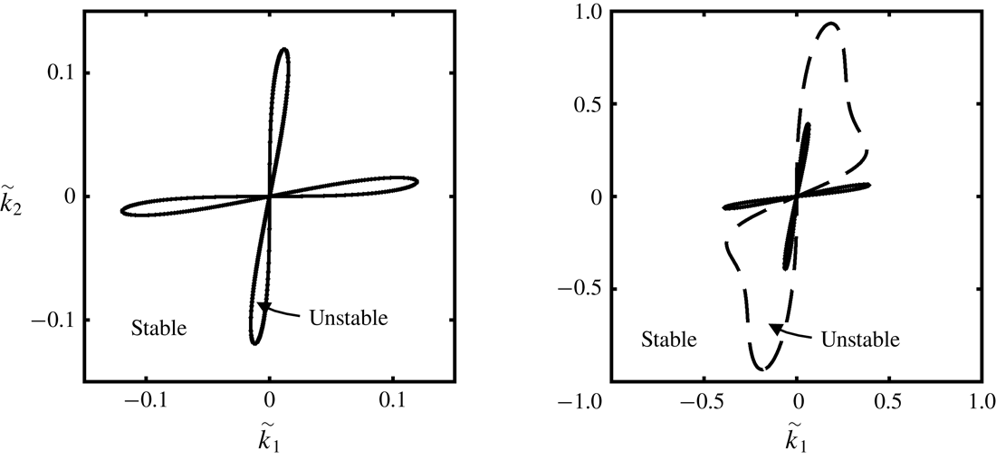
Contour plots of the dimensionless growth rate $\tilde{\unicode[STIX]{x1D706}}=A^{2}d^{2}\unicode[STIX]{x1D719}\unicode[STIX]{x1D70C}_{s}\unicode[STIX]{x1D706}/\unicode[STIX]{x1D702}^{0}$ as a function of the dimensionless wave vector $\tilde{k}_{i}=Adk_{i}$ for pure shearing and $I^{0}=0.001$ , calculated using (3.22) for (a) the NGF model and (b) the LI rheology. In both cases, the $\unicode[STIX]{x1D707}_{loc}(I)$ function (1.3) is used with the parameters $\unicode[STIX]{x1D707}_{s}=0.3819$ , $\unicode[STIX]{x1D707}_{2}=0.6435$ and $b=0.9377$ (so that $I_{0}=(\unicode[STIX]{x1D707}_{2}-\unicode[STIX]{x1D707}_{s})/b=0.279$ ). The white regions represent positive growth rates and linear instability, and solid lines represent the stability threshold. In (a), the dashed circle represents the cutoff wave vector magnitude, $\tilde{k}_{cut}$ , beyond which perturbations are stable for all wave vector directions.

To this point, the specific form of the $\unicode[STIX]{x1D707}_{loc}(I)$ function – which enters the NGF model through (2.6) and (2.7) and the growth rate (3.22) through $\unicode[STIX]{x1D708}^{0}$ – has been left unspecified. We begin by considering the Jop et al. (Reference Jop, Forterre and Pouliquen2005) form (1.3) and utilize their well-established parameters for glass beads: $\unicode[STIX]{x1D707}_{s}=0.3819$ , $\unicode[STIX]{x1D707}_{2}=0.6435$ and $b=0.9377$ , so that $I_{0}=(\unicode[STIX]{x1D707}_{2}-\unicode[STIX]{x1D707}_{s})/b=0.279$ . A contour plot of the growth rate, $\tilde{\unicode[STIX]{x1D706}}$ , as a function of the wave vector $\tilde{k}_{i}=Adk_{i}$ , calculated using (3.22), is shown in figure 1(a) for a quasi-static base-state inertial number of $I^{0}=0.001$ . The value of $I^{0}=0.001$ is chosen since it is illustrative of unstable behaviour when it occurs. The white regions represent positive growth rates – and hence linear instability and the loss of ellipticity – and solid lines denote the stability threshold. Figure 1(a) shows that the unstable region is confined to a set of finite wave vector magnitudes near the origin in wave vector space. Therefore, in the limit $|\boldsymbol{k}|\rightarrow \infty$ , perturbations are stable for all wave vector directions, and Hadamard instability does not arise, consistent with (3.18). A corresponding contour plot of the growth rate for the LI rheology, calculated by neglecting the terms involving $\tilde{k}$ in (3.23), is shown in figure 1(b) – which matches the result of Barker et al. (Reference Barker, Schaeffer, Bohorquez and Gray2015). In this case, the unstable regions extend to infinitely large wave vector magnitudes with corresponding growth rates that diverge to positive infinity, consistent with Hadamard instability. In comparing figures 1(a) and (b), we note that they are similar near the origin, since the addition of non-local terms has little effect on long-wavelength perturbations. In both cases, instability only occurs for wave vector directions within the ranges of approximately $\pm 34$ – $45^{\circ }$ with respect to the $\boldsymbol{e}_{1}$ -direction with the maximum positive growth rate occurring at angles of approximately $\pm 39^{\circ }$ . However, as the wave vector magnitude increases, the presence of the non-local terms in the NGF model leads to a wave vector cutoff, $k_{cut}$ , beyond which perturbations are stable for all wave vector directions. Importantly, since the quantity $2\unicode[STIX]{x03C0}/k_{cut}$ represents the smallest possible wavelength of an unstable perturbation, the wave vector cutoff, $k_{cut}$ , quantifies the regularization imparted by the NGF model. We define the dimensionless wave vector cutoff as $\tilde{k}_{cut}=Adk_{cut}$ – which is illustrated by the dashed circle in figure 1(a) – and note that $\tilde{k}_{cut}$ can depend on the material parameters $\{\unicode[STIX]{x1D707}_{s},\unicode[STIX]{x1D707}_{2},b\}$ and the base-state inertial number, $I^{0}$ , but not the non-local amplitude, $A$ . Then, since $k_{cut}=\tilde{k}_{cut}/Ad$ , the dimensional cutoff wave vector is inversely proportional to $A$ and the grain size, $d$ , so that $k_{cut}$ may be made arbitrarily small by taking $Ad$ to be arbitrarily large.

Figure 2.

(a) Contour plot of the cutoff wave vector magnitude, $\tilde{k}_{cut}$ , for pure shearing as a function of $(\unicode[STIX]{x1D707}_{2}-\unicode[STIX]{x1D707}_{s})$ and $I^{0}/I_{0}$ using the $\unicode[STIX]{x1D707}_{loc}(I)$ function (1.3) with $\unicode[STIX]{x1D707}_{s}=0.3819$ fixed. The white region bounded by the solid black line denotes states in which perturbations are stable for all wave vectors, and hence $\tilde{k}_{cut}=0$ in this region. (b) The quasi-static limit of the wave vector cutoff, $\tilde{k}_{cut}(I^{0}/I_{0}\rightarrow 0)$ , as a function of the static yield value, $\unicode[STIX]{x1D707}_{s}$ . (c) Cutoff wave vector magnitude, $\tilde{k}_{cut}$ , as a function of $bI^{0}$ using the Bingham-like $\unicode[STIX]{x1D707}_{loc}(I)$ function (1.2) with $\unicode[STIX]{x1D707}_{s}=0.3819$ fixed. Again, the range of $bI^{0}$ in which $\tilde{k}_{cut}=0$ represents states in which perturbations are stable for all wave vectors.

Next, we illustrate the effect of the material parameters $\{\unicode[STIX]{x1D707}_{s},\unicode[STIX]{x1D707}_{2},b\}$ and the base-state inertial number, $I^{0}$ , on $\tilde{k}_{cut}$ . Figure 2(a) shows a contour plot of $\tilde{k}_{cut}$ as a function of $(\unicode[STIX]{x1D707}_{2}-\unicode[STIX]{x1D707}_{s})$ and $I^{0}/I_{0}$ (where $I_{0}=(\unicode[STIX]{x1D707}_{2}-\unicode[STIX]{x1D707}_{s})/b$ ) with $\unicode[STIX]{x1D707}_{s}=0.3819$ fixed. We note that for $\unicode[STIX]{x1D707}_{s}=0.3819$ and the range of $(\unicode[STIX]{x1D707}_{2}-\unicode[STIX]{x1D707}_{s})$ considered in figure 2(a), $\unicode[STIX]{x1D707}_{loc}(I^{0})<1$ , so that the requirement (3.19) is always satisfied. The white region bounded by the solid black line represents combinations of material parameters and base states in which perturbations are stable for all wave vectors – and hence $\tilde{k}_{cut}=0$ – and is identical to the region of well-posed behaviour for the LI rheology (see figure 2 of Barker et al. (Reference Barker, Schaeffer, Bohorquez and Gray2015)). Outside this region, unstable behaviour of the type illustrated in figure 1(a) is observed, and $\tilde{k}_{cut}$ is non-zero. First, we discuss the quasi-static limit of $I^{0}/I_{0}\rightarrow 0$ . Using (3.6), $\unicode[STIX]{x1D708}^{0}\rightarrow bI^{0}/\unicode[STIX]{x1D707}_{s}$ , and using (3.23), $r^{0}\rightarrow 1/(1+\tilde{k}^{2}/\unicode[STIX]{x1D707}_{s})$ and $q^{0}\rightarrow \unicode[STIX]{x1D707}_{s}$ , so that the growth rate as a function of wave vector (3.22) – and hence $\tilde{k}_{cut}$ – only depends on the static yield value, $\unicode[STIX]{x1D707}_{s}$ . For $\unicode[STIX]{x1D707}_{s}=0.3819$ , $\tilde{k}_{cut}(I^{0}/I_{0}\rightarrow 0)=0.123$ , which may be observed in the lower portion of figure 2(a). The quasi-static wave vector cutoff value is important because it is indicative of $\tilde{k}_{cut}$ over a wide range of base-state inertial numbers $I^{0}/I_{0}\lesssim 0.1$ – i.e. $0\leqslant \tilde{k}_{cut}\lesssim 0.2$ for $I^{0}/I_{0}\lesssim 0.1$ in figure 2(a). The quasi-static limit of the wave vector cutoff, $\tilde{k}_{cut}(I^{0}/I_{0}\rightarrow 0)$ , is plotted as a function of the static yield value, $\unicode[STIX]{x1D707}_{s}$ , in figure 2(b), showing that this quantity increases monotonically with $\unicode[STIX]{x1D707}_{s}$ and that as $\unicode[STIX]{x1D707}_{s}\rightarrow 0$ , the wave vector cutoff goes to zero, and unstable behaviour disappears (consistent with Barker & Gray (Reference Barker and Gray2017)). Then, returning to figure 2(a), as the base-state inertial number is increased beyond $I^{0}/I_{0}\approx 1$ , $\tilde{k}_{cut}$ rapidly increases – exceeding the upper limit of the contour plot. Mathematically, this is because the cooperativity length of the NGF model decays as the base-state inertial number increases, and non-local effects play a decreasing role in this limit. While $\tilde{k}_{cut}$ remains finite and the Hadamard instability does not occur in this range, unstable perturbations of very short wavelength (but finite growth rate) arise, indicating that the NGF model will predict narrow flow localization features, which to our knowledge are not observed experimentally in rapid flows. For context, the NGF model was proposed to address the shortcomings of the LI rheology in the quasi-static and dense inertial flow regimes ( $I\lesssim 10^{-1}$ ). Therefore, in order to provide a more physical regularization of the LI rheology in the rapid flow regime, it will be necessary to include additional physics not currently present in the NGF model.

Finally, to demonstrate that the observations discussed in this section are not limited to the specific choice of the $\unicode[STIX]{x1D707}_{loc}(I)$ function (1.3), we consider the stability of the NGF model using the Bingham-like form of the $\unicode[STIX]{x1D707}_{loc}(I)$ function (1.2). Figure 2(c) shows a plot of $\tilde{k}_{cut}$ as a function of $bI^{0}$ with $\unicode[STIX]{x1D707}_{s}=0.3819$ fixed. Since (1.2) does not possess an upper limiting value, we only consider a range of $bI^{0}$ in which $\unicode[STIX]{x1D707}_{loc}(I^{0})<1$ , so that $bI^{0}<1-\unicode[STIX]{x1D707}_{s}=0.6181$ and (3.19) is satisfied. Again, we observe the quasi-static limit of the wave vector cutoff, i.e. $\tilde{k}_{cut}(I^{0}/I_{0}\rightarrow 0)=0.123$ for $\unicode[STIX]{x1D707}_{s}=0.3819$ . Then, as $bI^{0}$ is increased, $\tilde{k}_{cut}$ remains near the quasi-static limit until it quickly decreases to zero around $bI^{0}=0.0158$ . For $0.0158\leqslant bI^{0}<0.6181$ , perturbations are stable for all wave vectors. Therefore, the stability of the NGF model in the quasi-static and dense inertial flow regimes ( $I\lesssim 10^{-1}$ ) is similar for both choices of the $\unicode[STIX]{x1D707}_{loc}(I)$ function, (1.2) and (1.3).

4 Nonlinear numerical simulations of strain localization in plane-strain compression

In this section, we illustrate that a consequence of the finite-wavelength linear instability detected in § 3 is the potential for diffuse localization to arise in fully nonlinear, quasi-static solutions. To this end, we apply the NGF model to the case of plane-strain (biaxial) compression of a dense granular material – a common configuration for studying strain localization in both experiments (e.g. Han & Drescher Reference Han and Drescher1993; Desrues & Viggiani Reference Desrues and Viggiani2004; Rechenmacher Reference Rechenmacher2006; Le Bouil et al. Reference Le Bouil, Amon, McNamara and Crassous2014; Houdoux et al. Reference Houdoux, Nguyen, Amon and Crassous2018) and continuum simulations (e.g. Anand & Gu Reference Anand and Gu2000; Al Hattamleh et al. Reference Al Hattamleh, Muhunthan and Zbib2004; Gao & Zhao Reference Gao and Zhao2013), since the geometry allows plastic deformation to localize into a shear band with minimal interference from the boundary conditions. From the outset, we recognize that the process of strain localization into shear bands is quite complex; in particular, the initial state has an important impact on shear-band formation. If the granular material is over-consolidated, it will dilate during the beginning stages of quasi-static shear deformation, leading to shear softening, which contributes to strain localization. Conversely, an initially under-consolidated granular material undergoes compaction and attendant shear hardening, which counteracts localization. It is well appreciated that dilatancy and shear softening/hardening have a quantitative impact on the formation and orientation of shear bands in the quasi-static regime (Rudnicki & Rice Reference Rudnicki and Rice1975). Moreover, the initial contact fabric and its evolution play a role in quasi-static deformation of dense granular materials (Sun & Sundaresan Reference Sun and Sundaresan2011), which can have a further effect on the process of strain localization (Gao & Zhao Reference Gao and Zhao2013). Continuum models that account for dilatancy and associated shear softening/hardening (e.g. Schofield & Wroth Reference Schofield and Wroth1968; Anand & Gu Reference Anand and Gu2000) as well as fabric evolution (e.g. Nemat-Nasser Reference Nemat-Nasser2004; Sun & Sundaresan Reference Sun and Sundaresan2011; Gao & Zhao Reference Gao and Zhao2013) have been developed in the literature, but at present, non-local rheological models for dense granular flow do not incorporate these effects. Therefore, the intent of this section is not to quantitatively capture experimental observations of localization but instead to demonstrate a link between linear instability and the bifurcation of homogeneous deformation to diffuse localization in fully nonlinear settings.

Figure 3.

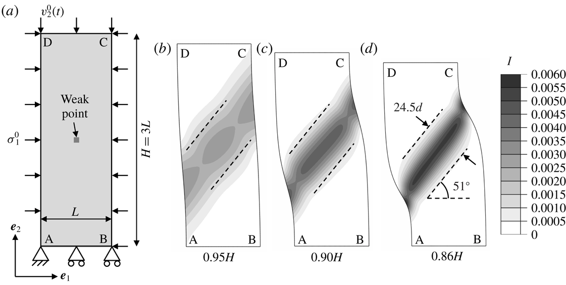
(a) Schematic of the computational domain used in finite-element simulations of plane-strain compression of a dense granular material. (b–d) Contours of the inertial number field for a specimen size of $L=40d$ , a quasi-static target inertial number of $I^{0}=0.001$ and a mesh resolution of $d/2$ . The deformed distance between faces AB and CD is (b) $0.95H$ , (c) $0.90H$ and (d) $0.86H$ .

We consider the configuration shown in figure 3(a), consisting of a rectangular box of dense granular material with dimensions $L$ and $H=3L$ in the $x_{1}$ - and $x_{2}$ -directions, respectively, subjected to plane-strain compression along the $x_{2}$ -direction. Regarding the mechanical boundary conditions, the bottom face AB is fixed in the $x_{2}$ -direction, $v_{2}=0$ , and the corner A is pinned to prevent lateral free-body motion, $v_{1}=v_{2}=0$ . The lateral faces AD and BC are subjected to a compressive normal stress $\unicode[STIX]{x1D70E}_{1}^{0}<0$ , which continues to act normal to the faces as the surface orientation evolves with deformation, and the top face CD is moved downward at a velocity $v_{2}^{0}(t)<0$ . For a given lateral normal stress, $\unicode[STIX]{x1D70E}_{1}^{0}$ , the downward velocity, $v_{2}^{0}(t)$ , is chosen to obtain a target inertial number, $I^{0}$ , supposing homogeneous deformation, as follows. In homogeneous, constant-volume, plane-strain compression, denote the normal stresses as $\unicode[STIX]{x1D70E}_{1}^{0}<0$ , $\unicode[STIX]{x1D70E}_{2}^{0}<\unicode[STIX]{x1D70E}_{1}^{0}$ and $\unicode[STIX]{x1D70E}_{3}^{0}=(\unicode[STIX]{x1D70E}_{1}^{0}+\unicode[STIX]{x1D70E}_{2}^{0})/2$ , so that $\unicode[STIX]{x1D70F}^{0}=(\unicode[STIX]{x1D70E}_{1}^{0}-\unicode[STIX]{x1D70E}_{2}^{0})/2$ , $P^{0}=-(\unicode[STIX]{x1D70E}_{1}^{0}+\unicode[STIX]{x1D70E}_{2}^{0})/2$ and $\unicode[STIX]{x1D707}^{0}=\unicode[STIX]{x1D70F}^{0}/P^{0}$ . Next, using this information, for a given $\unicode[STIX]{x1D70E}_{1}^{0}$ and $I^{0}$ , $P^{0}$ may be determined by way of the $\unicode[STIX]{x1D707}_{loc}(I)$ function as $P^{0}=-\unicode[STIX]{x1D70E}_{1}^{0}/(1-\unicode[STIX]{x1D707}_{loc}(I^{0}))$ . Similarly, denote the normal strain rates as $D_{1}^{0}>0$ , $D_{2}^{0}=-D_{1}^{0}$ and $D_{3}^{0}=0$ , so that $\dot{\unicode[STIX]{x1D6FE}}^{0}=-2D_{2}^{0}$ . Then, using the definition of the inertial number, we have that the strain rate along the direction of compression should be $D_{2}^{0}=-(I^{0}/2)\sqrt{P^{0}/d^{2}\unicode[STIX]{x1D70C}_{s}}$ . To achieve this constant, target value of $D_{2}^{0}$ – i.e. a constant true strain rate – we set the top surface velocity to be $v_{2}^{0}(t)=D_{2}^{0}H\exp (D_{2}^{0}t)$ , where $v_{2}^{0}(t)$ is time dependent since the specimen height evolves with deformation and downward since $D_{2}^{0}<0$ . For the granular fluidity boundary conditions, based on the experience built up in our past work (Henann & Kamrin Reference Henann and Kamrin2013, Reference Henann and Kamrin2014a ; Liu & Henann Reference Liu and Henann2017), we invoke homogeneous Neumann boundary conditions on all boundaries. Finally, we introduce a centrally located weak point by modifying the static yield value of a single element – indicated in figure 3(a) – to be $0.99\unicode[STIX]{x1D707}_{s}$ . This point serves as a potential nucleation point for localization. In summary, we specify boundary conditions consistent with homogeneous flow at a target inertial number, $I^{0}$ . Our expectation is that if the governing equations are linearly stable, the imperfection will have no effect, and homogeneous flow will proceed. However, for values of $I^{0}$ corresponding to linear instability, we expect that the imperfection will trigger a bifurcation of homogeneous flow to flow localization in a shear band.

Consistent with our interest in quasi-static solutions, we use the Bingham-like form of the $\unicode[STIX]{x1D707}_{loc}(I)$ function (1.2) throughout this section along with dimensionless material parameters for glass beads. Namely, the local parameters are taken to be $\unicode[STIX]{x1D707}_{s}=0.3819$ and $b=0.9377$ , and the non-local amplitude was calibrated in our previous work to be $A=0.48$ (Henann & Kamrin Reference Henann and Kamrin2013). To obtain numerical solutions, we utilize the nonlinear, quasi-static finite-element formulation of the NGF model developed and described in detail in our previous work (Henann & Kamrin Reference Henann and Kamrin2016) and implemented in the commercial finite-element program Abaqus (2017). We note that our implementation includes a stiff elastic response, which we have verified does not affect any of the subsequently reported calculation results. The finite-element degrees of freedom are the in-plane displacement components – rather than velocity components – and the granular fluidity. (See Henann & Kamrin (Reference Henann and Kamrin2016) for further discussion of this point.) We begin by considering a specimen size of $L=40d$ , a quasi-static target inertial number of $I^{0}=0.001$ and a mesh resolution of $d/2$ (19 200 elements). Figures 3(b), 3(c) and 3(d) show contour plots of the inertial number field on the deformed shape after the specimen has been compressed to the point that the deformed distance between faces AB and CD is $0.95H$ , $0.90H$ and $0.86H$ , respectively. (Under homogeneous deformation, these boundary displacements would correspond to true strains of $-0.05$ , $-0.10$ and $-0.15$ .) Consistent with expectation, homogeneous deformation does not occur. After a small amount of compressive strain, flow localizes into a single shear band, which persists as further deformation is applied. The inertial number field is greater than $I^{0}$ inside the shear band, while $I$ is less than $I^{0}$ in regions outside the shear band but never exactly zero. The important features of the shear band are its orientation and its width, which evolve minimally over the range of deformation shown in figure 3(b–d). Making a connection with the linear stability analysis of § 3.3, the perturbations with the maximum positive growth rate in the quasi-static regime correspond to wave vector directions of approximately $\pm 39^{\circ }$ with respect to the $\boldsymbol{e}_{1}$ -direction. Since the wave vector direction represents the direction normal to localization bands, shear bands are expected to form at angles of either $51^{\circ }$ or $-51^{\circ }$ . The dashed lines sketched in figure 3(b–d) are at an angle of $51^{\circ }$ with respect to the horizontal, illustrating that the simulated shear-band orientation is indeed consistent with the orientation suggested by the linear stability analysis. Regarding the shear-band width, we recall that the quantity $2\unicode[STIX]{x03C0}/k_{cut}$ represents the smallest possible wavelength of an unstable perturbation. Since the quasi-static limit of the wave vector cutoff is $\tilde{k}_{cut}=0.123$ for $\unicode[STIX]{x1D707}_{s}=0.3819$ , the corresponding cutoff wavelength is $2\unicode[STIX]{x03C0}/k_{cut}=2\unicode[STIX]{x03C0}Ad/\tilde{k}_{cut}=24.5d$ for $A=0.48$ . The pairs of parallel dashed lines sketched in figure 3(b–d) are spaced $24.5d$ apart, illustrating that the simulated width of the shear band is indeed of the same order as the unstable wavelength cutoff. Therefore, the regularization provided by the NGF model sets the diffuse width of shear bands that follow from the linear instability.

Figure 4.

Contours of the inertial number field for a target inertial number of $I^{0}=0.001$ , a mesh resolution of $d/2$ and specimen sizes of (a) $L=20d$ , (b) $L=40d$ and (c) $L=60d$ . The deformed distance between faces AB and CD is $0.90H$ for each case.

To demonstrate that the results of figure 3(b–d) are primarily due to the material response – i.e. material instability – and not to the geometry of the specimen, we consider several specimen sizes while keeping the aspect ratio fixed. Figures 4(a), 4(b) and 4(c) show contour plots of the inertial number field on the deformed shape for $L=20d$ , $40d$ and $60d$ , respectively. In all three cases, the deformed distance between faces AB and CD is $0.90H$ , where $H$ represents the respective specimen height, $H=3L$ , for each case. For reference, the contour plots of figure 3(c) and figure 4(b) are identical. For the smaller specimen size of $L=20d$ shown in figure 4(a), the shear band is clearly influenced by the boundaries of the specimen, since the shear-band width is comparable to the specimen size. Comparing the cases of $L=40d$ and $L=60d$ shown in figure 4(b,c), some boundary effects are apparent, but the shear-band widths and angles are quite similar. This is illustrated by the parallel dashed lines in figure 4(b,c), which are oriented at an angle of $51^{\circ }$ with respect to the horizontal and spaced $24.5d$ apart. This observation indicates that so long as the specimen is sufficiently large, boundary effects are secondary in plane-strain compression, and the observed shear-band features may be attributed to the intrinsic material response.

Figure 5.

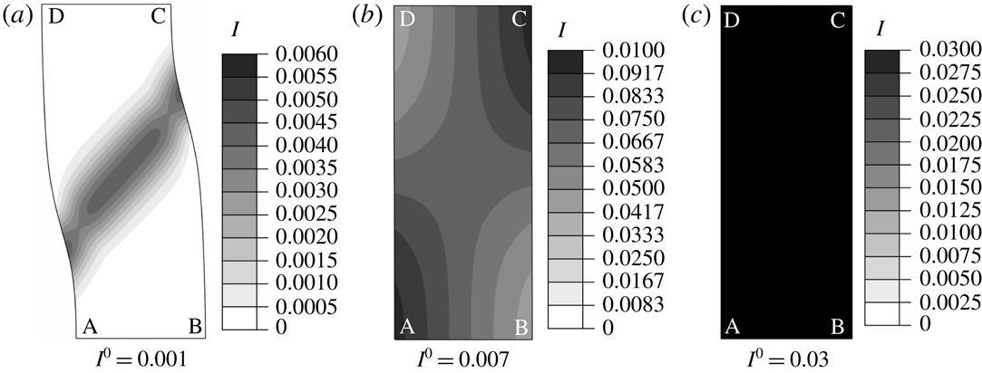
Contours of the inertial number field for a specimen size of $L=40d$ , a mesh resolution of $d/2$ and target inertial numbers of (a) $I^{0}=0.001$ , (b) $I^{0}=0.007$ and (c) $I^{0}=0.03$ . The deformed distance between faces AB and CD is $0.90H$ .

Next, we consider the effect of the target inertial number, $I^{0}$ , focusing on the specific cases of $I^{0}=0.001$ , $0.007$ and $0.03$ . With reference to the cutoff wave vector magnitude, $\tilde{k}_{cut}$ , determined in the linear stability analysis of § 3.3 and shown in figure 2(c), these choices correspond to target base states in the quasi-static plateau regime, the transition regime and the stable, dense inertial regime, respectively. Figure 5(a–c) shows contour plots of the inertial number field on the deformed shape for $I^{0}=0.001$ , $0.007$ and $0.03$ , a fixed specimen size of $L=40d$ and a mesh resolution of $d/2$ . As before, the deformed distance between faces AB and CD is $0.90H$ . The contour plots of figures 3(c) and 5(a) are identical, showing a clear shear band in the quasi-static regime. For the higher target inertial number of $I^{0}=0.007$ , a distinct shear band does not form, but flow remains slightly inhomogeneous. Making a connection with the linear stability analysis, we associate this change with the lower value of $\tilde{k}_{cut}$ for $I^{0}=0.007$ – or equivalently, the larger value of the unstable wavelength cutoff, $2\unicode[STIX]{x03C0}/k_{cut}$ . We note that since only long wavelengths are linearly unstable for this case, the specimen size does have an influence on the inertial number field. When $I^{0}$ is increased further to 0.03, flow is homogeneous at the target inertial number. This is due to the unconditionally stable behaviour for this base state, which precludes the imperfection from triggering a bifurcation into inhomogeneous flow – consistent with expectation. Therefore, inhomogeneous flow and localization do not arise when the target inertial number, $I^{0}$ , is in the regime in which the quasi-static governing equations are elliptic, exhibiting no linear instability of any wavelength.

Figure 6.

Contours of the inertial number field for a specimen size of $L=40d$ , a target inertial number of $I^{0}=0.001$ and mesh resolutions of (a) $2d$ , (b) $d$ , (c) $d/2$ and (d) $d/4$ . The deformed distance between faces AB and CD is $0.90H$ . The NGF model predicts diffuse and mesh-size-independent shear-band widths.

Figure 7.

Contours of the inertial number field for a specimen size of $L=40d$ , a target inertial number of $I^{0}=0.001$ and mesh resolutions of (a) $2d$ , (b) $d$ , (c) $d/2$ and (d) $d/4$ , calculated using the LI rheology rather than the NGF model. The deformed distance between faces AB and CD is approximately $0.99H$ .

Finally, we verify that the simulation results for the NGF model presented in this section are independent of mesh resolution. Returning to the case of $L=40d$ and $I^{0}=0.001$ , contour plots of the inertial number field on the deformed shape are shown in figure 6 for mesh resolutions of $2d$ , $d$ , $d/2$ and $d/4$ (1200, 4800, 19 200 and 76 800 elements, respectively). As before, the deformed distance between faces AB and CD is $0.90H$ . As the mesh resolution is refined, the inertial number field converges to a resolution-independent solution of a diffuse shear band. For comparison, we have also calculated corresponding solutions using the LI rheology. We continue to consider $L=40d$ , $I^{0}=0.001$ and mesh resolutions of $2d$ , $d$ , $d/2$ and $d/4$ but only a small amount of boundary displacement in which the deformed distance between faces AB and CD is about $0.99H$ . Contour plots of the inertial number field on the deformed shape are shown in figure 7 for each mesh resolution. Using the LI rheology, localization into shear bands is observed. The dashed lines sketched in figure 7(d) are at angles of $\pm 51^{\circ }$ with respect to the horizontal, illustrating that – like the NGF model – the simulated shear-band orientation is consistent with the orientation suggested by the linear stability analysis. However, in contrast to results obtained using the NGF model, shear bands are sharp with intense shearing present inside the bands and the inertial number equal to zero outside the bands. As the mesh is refined, the widths of shear bands do not approach exactly zero, instead sharpening to a point at which the inertial number inside the bands is of the order of $10^{-2}$ (which is approximately the lower bound of the linearly stable, dense inertial regime for the LI rheology using the current set of material parameters). That said, shear bands are quite sharp and require a very high mesh resolution to resolve. Moreover, in spite of the centrally located imperfection, multiple shear bands are observed with the number of bands increasing as the mesh is refined, and the shear bands tend to move spatially as deformation progresses, never coalescing into a single, persistent shear band. These observations may be interpreted as symptoms of the Hadamard-type linear instability exhibited by the LI rheology.

5 Linear stability of the IG model

The success of the NGF model as well as the velocity-gradient model of Goddard & Lee (Reference Goddard and Lee2017) in suppressing the Hadamard instability and providing a regularization of the LI rheology poses the question of whether other gradient extensions of the LI rheology lead to similar results. In this section, we apply a linear stability analysis analogous to that described in § 3 to the IG model proposed by Bouzid et al. (Reference Bouzid, Trulsson, Claudin, Clément and Andreotti2013). The model as described by Bouzid et al. (Reference Bouzid, Trulsson, Claudin, Clément and Andreotti2013) is one-dimensional in form and modifies the LI rheology (1.1) through a gradient expansion involving the Laplacian of the inertial number in the following manner:

(5.1) $$\begin{eqnarray}\displaystyle \unicode[STIX]{x1D707}=\unicode[STIX]{x1D707}_{loc}(I)\left(1-\frac{\unicode[STIX]{x1D708}_{I}d^{2}}{I}\frac{\unicode[STIX]{x2202}^{2}I}{\unicode[STIX]{x2202}x_{k}\unicode[STIX]{x2202}x_{k}}\right), & & \displaystyle\end{eqnarray}$$

where $\unicode[STIX]{x1D708}_{I}$ is a dimensionless material constant, which plays a similar role to the non-local amplitude, $A$ , in the NGF model. The IG model (5.1) has been successfully applied to capturing flow fields in the quasi-static regime in several statically determinate, inhomogeneous, one-dimensional flow configurations (Bouzid et al. Reference Bouzid, Trulsson, Claudin, Clément and Andreotti2013, Reference Bouzid, Trulsson, Claudin, Clément and Andreotti2015b ; Tang et al. Reference Tang, Brzinski, Shearer and Daniels2018). To proceed, it is necessary to generalize (5.1) to a tensorial form. We follow the precedent of Jop et al. (Reference Jop, Forterre and Pouliquen2006) for the LI rheology and Henann & Kamrin (Reference Henann and Kamrin2013) for the NGF model and assume (1) constant-volume steady flow and (2) co-directionality of the strain-rate tensor and the stress deviator, so that the Cauchy stress tensor is given by

(5.2) $$\begin{eqnarray}\displaystyle \unicode[STIX]{x1D70E}_{ij}=-P\unicode[STIX]{x1D6FF}_{ij}+\sqrt{2}\unicode[STIX]{x1D707}_{loc}(I)P\left(1-\frac{\unicode[STIX]{x1D708}_{I}d^{2}}{I}\frac{\unicode[STIX]{x2202}^{2}I}{\unicode[STIX]{x2202}x_{k}\unicode[STIX]{x2202}x_{k}}\right)\unicode[STIX]{x1D615}_{ij}, & & \displaystyle\end{eqnarray}$$

where, as in § 2, $\unicode[STIX]{x1D60B}_{ij}=(1/2)(\unicode[STIX]{x2202}v_{i}/\unicode[STIX]{x2202}x_{j}+\unicode[STIX]{x2202}v_{j}/\unicode[STIX]{x2202}x_{i})$ is the symmetric and deviatoric strain-rate tensor, $\dot{\unicode[STIX]{x1D6FE}}=(2\unicode[STIX]{x1D60B}_{ij}\unicode[STIX]{x1D60B}_{ij})^{1/2}$ is the equivalent shear strain rate, $\unicode[STIX]{x1D615}_{ij}=\sqrt{2}\unicode[STIX]{x1D60B}_{ij}/\dot{\unicode[STIX]{x1D6FE}}$ is the direction of flow, $P$ is the pressure and $I=\dot{\unicode[STIX]{x1D6FE}}\sqrt{d^{2}\unicode[STIX]{x1D70C}_{s}/P}$ is the inertial number. Then, continuing to use the definitions $\unicode[STIX]{x1D70F}=(\unicode[STIX]{x1D70E}_{ij}^{\prime }\unicode[STIX]{x1D70E}_{ij}^{\prime }/2)^{1/2}$ and $\unicode[STIX]{x1D707}=\unicode[STIX]{x1D70F}/P$ , the three-dimensional constitutive equation (5.2) implies the constitutive equation (5.1) in terms of invariant quantities. We note that (5.2) bears some relation to the velocity-gradient model of Goddard & Lee (Reference Goddard and Lee2017) in that it explicitly includes higher-order gradients of kinematic quantities – i.e. it is a weakly non-local, gradient–viscoplastic model – but differs in that the gradient term depends on the velocity field in a nonlinear manner and also involves the pressure field. Moreover, unlike the model of Goddard & Lee (Reference Goddard and Lee2017), the IG model has not been formulated in a thermodynamically consistent manner, and hence positive dissipation is not ensured. Finally, we acknowledge that there are certainly other possible paths to generalize (5.1) to a tensorial setting that eschew co-directionality; however, co-directionality represents a straightforward first approach to generalizing a scalar rheology to tensorial form. The equations of incompressibility, $\unicode[STIX]{x2202}v_{j}/\unicode[STIX]{x2202}x_{j}=0$ , the stress constitutive equation (5.2) and the equations of motion (2.2) then represent a closed system of equations.

In appendix C, the governing equations of the IG model are linearized about a base state of steady, homogeneous, constant-volume flow, and the ellipticity of the linearized equations is considered. The resulting eigenvalue problem for the IG model has the same form as that obtained for the NGF model, (3.15) and (3.16), with one key difference: the expressions for $r^{0}$ and $q^{0}$ are different and given by

(5.3a,b ) $$\begin{eqnarray}\displaystyle r^{0}(\boldsymbol{k})=1-\unicode[STIX]{x1D708}^{0}-\unicode[STIX]{x1D708}_{I}d^{2}|\boldsymbol{k}|^{2}\quad \text{and}\quad q^{0}(\boldsymbol{k})=\unicode[STIX]{x1D707}_{loc}(I^{0})\left(1-{\textstyle \frac{1}{2}}\unicode[STIX]{x1D708}^{0}-{\textstyle \frac{1}{2}}\unicode[STIX]{x1D708}_{I}d^{2}|\boldsymbol{k}|^{2}\right)\!.\quad & & \displaystyle\end{eqnarray}$$

In the long-wavelength limit ( $|\boldsymbol{k}|\rightarrow 0$ ), both (3.13) and (5.3) reduce to the wave-vector-independent forms derived by Barker et al. (Reference Barker, Schaeffer, Bohorquez and Gray2015) for the LI rheology. However, in the short-wavelength limit ( $|\boldsymbol{k}|\rightarrow \infty$ ), for the IG model, $r^{0}$ and $q^{0}$ are dominated by the $|\boldsymbol{k}|^{2}$ terms in (5.3) and diverge to negative infinity, rather than remaining bounded as their NGF model counterparts (3.17). This behaviour is especially problematic for $q^{0}$ , since we can no longer ensure that the denominator in (3.16) remains positive. Therefore, situations in which $(|\boldsymbol{k}|^{2}-\sqrt{2}q^{0}(\boldsymbol{k})k_{m}\unicode[STIX]{x1D615}_{mn}^{0}k_{n})=0$ are unavoidable, and growth rates that diverge to infinity for finite wave vector magnitudes are to be expected. Moreover, the presence of the gradient terms in the IG model does not guarantee that Hadamard instability is suppressed. In the limit $|\boldsymbol{k}|\rightarrow \infty$ , the tensor $\unicode[STIX]{x1D608}_{ik}$ behaves asymptotically as

(5.4) $$\begin{eqnarray}\displaystyle \unicode[STIX]{x1D608}_{ik}(\boldsymbol{k})\sim \frac{2\sqrt{2}}{\unicode[STIX]{x1D707}_{loc}(I^{0})}\left[k_{i}-\left(\frac{|\boldsymbol{k}|^{2}}{k_{m}\unicode[STIX]{x1D615}_{mn}^{0}k_{n}}\right)\unicode[STIX]{x1D615}_{ij}^{0}k_{j}\right]\unicode[STIX]{x1D615}_{kl}^{0}k_{l}-|\boldsymbol{k}|^{2}\unicode[STIX]{x1D6FF}_{ik}. & & \displaystyle\end{eqnarray}$$

In contrast to (3.18), (5.4) is not negative definite for all wave vector directions, and as we shall show momentarily for the case of pure shearing, eigenvalues of (5.4) can diverge to positive infinity for certain directions. Finally, the non-local material parameter, $\unicode[STIX]{x1D708}_{I}$ , does not appear in (5.4), indicating that increasing the value of $\unicode[STIX]{x1D708}_{I}$ will not alleviate Hadamard-type instability when it arises.

Figure 8.

Contour plots of the dimensionless growth rate $\tilde{\unicode[STIX]{x1D706}}=\unicode[STIX]{x1D708}_{I}d^{2}\unicode[STIX]{x1D719}\unicode[STIX]{x1D70C}_{s}\unicode[STIX]{x1D706}/\unicode[STIX]{x1D702}^{0}$ as a function of the dimensionless wave vector $\tilde{k}_{i}=\sqrt{\unicode[STIX]{x1D708}_{I}}dk_{i}$ for pure shearing and (a) $I^{0}=0.001$ and (b) $I^{0}=0.1$ , calculated using (3.22) for the IG model. In both cases, the $\unicode[STIX]{x1D707}_{loc}(I)$ function (1.3) is used with the parameters $\unicode[STIX]{x1D707}_{s}=0.3819$ , $\unicode[STIX]{x1D707}_{2}=0.6435$ and $b=0.9377$ (so that $I_{0}=(\unicode[STIX]{x1D707}_{2}-\unicode[STIX]{x1D707}_{s})/b=0.279$ ). The close-up in (a) shows the small unstable region near the origin in wave vector space. The white regions with dashed hatching represent positive growth rates that grow without bound as $\tilde{k}\rightarrow \infty$ – i.e. wave vectors along these directions exhibit Hadamard instability. Solid black lines represent the stability threshold $\tilde{\unicode[STIX]{x1D706}}=0$ , while solid grey lines denote contours over which $\tilde{\unicode[STIX]{x1D706}}$ is discontinuous.

To illustrate this behaviour, we consider a base state of steady, homogeneous, constant-volume pure shearing as described at the beginning of § 3.3. Introducing the dimensionless growth rate $\tilde{\unicode[STIX]{x1D706}}=\unicode[STIX]{x1D708}_{I}d^{2}\unicode[STIX]{x1D719}\unicode[STIX]{x1D70C}_{s}\unicode[STIX]{x1D706}/\unicode[STIX]{x1D702}^{0}$ and dimensionless wave vector $\tilde{k}_{i}=\sqrt{\unicode[STIX]{x1D708}_{I}}dk_{i}$ , the growth rate in pure shearing is given by (3.22) with $r^{0}(\tilde{k})=1-\unicode[STIX]{x1D708}^{0}-\tilde{k}^{2}$ and $q^{0}(\tilde{k})=\unicode[STIX]{x1D707}_{loc}(I^{0})(1-\unicode[STIX]{x1D708}^{0}/2-\tilde{k}^{2}/2)$ . For the $\unicode[STIX]{x1D707}_{loc}(I)$ function, we again consider the form (1.3) and utilize the parameters $\unicode[STIX]{x1D707}_{s}=0.3819$ , $\unicode[STIX]{x1D707}_{2}=0.6435$ and $b=0.9377$ . A contour plot of the growth rate, $\tilde{\unicode[STIX]{x1D706}}$ , as a function of the wave vector, $\tilde{k}_{i}$ , is shown in figure 8(a) for a quasi-static base-state inertial number of $I^{0}=0.001$ with positive growth rates denoted by white regions. The small unstable region near the origin in wave vector space shown in the close-up in figure 8(a) is actually quite similar to that shown in figure 1(a) – only appearing much smaller in the main figure because the domain of wave vectors in figure 8(a) is significantly larger than in figure 1(a). The difference in the contour plots of figures 8(a) and 1(a) arises as the wave vector magnitude increases. The white regions with dashed hatching far from the origin in figure 8(a) represent positive growth rates that grow without bound as $\tilde{k}\rightarrow \infty$ – i.e. wave vectors along these directions exhibit Hadamard instability. Moreover, while the solid black lines denote contours of $\tilde{k}=0$ , the solid grey lines denote contours along which $\tilde{k}^{2}-q^{0}(\tilde{k})(\tilde{k}_{1}^{2}-\tilde{k}_{2}^{2})=0$ . The growth rate is discontinuous across these contours, diverging to positive and negative infinity as the contour is approached from either side. Therefore, diverging growth rates are encountered for finite wave vector magnitudes. Figure 8(b) shows growth-rate contours for a higher base-state inertial number of $I^{0}=0.1$ , showing that while the unstable region near the origin disappears, the unstable behaviour for high wave vector magnitudes and the contours of growth-rate discontinuity remain. This is in contrast to both the LI rheology and the NGF model, which possess unconditionally stable behaviour for this case.

The results of this section’s linear stability analysis suggest that obtaining robust numerical solutions using the IG model in general flow geometries will be difficult. Indeed, previous applications of this model have been restricted to statically determinate, one-dimensional problems (Bouzid et al. Reference Bouzid, Trulsson, Claudin, Clément and Andreotti2013, Reference Bouzid, Trulsson, Claudin, Clément and Andreotti2015b ; Tang et al. Reference Tang, Brzinski, Shearer and Daniels2018), in which the stress field was known from the outset, and only the constitutive equation (5.1) was used to obtain solutions for the flow field – masking potential unstable behaviour. To understand the source of this mathematical behaviour, we note that unbounded growth rates stem from the manner in which $q^{0}$ depends on the wave vector magnitude. This dependence may be traced back to the term in the linearized equations of motion (C 6) involving higher-order pressure gradients, implying that this term has a deeply destabilizing effect. In fact, if this term in (C 6) and the consequent dependence of $q^{0}$ on the wave vector in (5.3) are neglected, unbounded growth rates do not arise, and Hadamard-type instability is successfully suppressed. Therefore, due to the involvement of pressure in the inertial number, developing a non-local rheology based on higher-order gradients of the inertial number that leads to well-posed governing equations will be challenging, and it seems unlikely that alternatives to co-directionality will significantly alter this conclusion.

6 Concluding remarks

In this work, we established that the NGF model regularizes the Hadamard-type instability of the LI rheology. In particular, by performing a linear stability analysis in which a base state of steady, homogeneous, constant-volume flow is subjected to perturbation, we showed that the NGF model provides a wave-vector-magnitude cutoff, beyond which all perturbations are stable and unbounded growth rates do not occur. Further, for certain wave vectors within the cutoff, linear instability of finite wavelength and bounded growth rate remains, which is a necessary condition for diffuse strain localization. We considered two specific forms of the $\unicode[STIX]{x1D707}_{loc}(I)$ function and a wide range of material parameters, showing that these observations are quite broad.

Second, to demonstrate the consequences of finite-wave-vector instability and the loss of ellipticity of the quasi-static governing equations, we carried out fully nonlinear finite-element simulations of plane-strain compression. Specifically, we showed that when boundary conditions consistent with a base state of homogeneous deformation in the unstable regime are applied, the NGF model predicts a bifurcation from homogeneous deformation to diffuse strain localization, but for a base state in the stable regime with higher inertial number, no bifurcation occurs. When localization occurs, the thicknesses of shear bands predicted by the NGF model were observed to be independent of the mesh resolution.

Lastly, we performed an analogous linear stability analysis on a tensorial generalization of the IG model of Bouzid et al. (Reference Bouzid, Trulsson, Claudin, Clément and Andreotti2013) and showed that due to the presence of higher-order pressure gradients in the constitutive equations, unbounded growth rates arise in pure shearing over a wide range of base-state inertial numbers – in contrast to both the LI rheology and the NGF model – illustrating that the inclusion of higher-order gradients of the inertial number in a constitutive model does not provide a straightforward path to well-posed governing equations.

In closing, we highlight two avenues along which the NGF model may be extended. First, as discussed at the beginning of § 4, the effect of the initial state, dilatancy and associated shear softening/hardening, as well as fabric and its evolution all have important impacts on the mechanics of dense granular materials in the quasi-static flow regime – particularly during the transition from static to flowing states. Moreover, dilatancy has been observed during steady, quasi-static flows (Krishnaraj & Nott Reference Krishnaraj and Nott2016). At present, the NGF model and other non-local rheological models cannot capture these effects. One approach to incorporating transient dilatancy and shear softening/hardening during developing flow into the NGF model is to introduce an evolution law for the solid packing fraction (e.g. Schofield & Wroth Reference Schofield and Wroth1968; Anand & Gu Reference Anand and Gu2000) and couple the local response function $g_{loc}$ to its evolution. Along this line, we note that the recent works of Barker et al. (Reference Barker, Schaeffer, Shearer and Gray2017) and Heyman et al. (Reference Heyman, Delannay, Tabuteau and Valance2017) have proposed compressible, dilatant extensions of the LI rheology as a route to well-posed governing equations. However, the conditions for well-posedness may be too restrictive to describe experiments in the quasi-static regime. Indeed, the recent work of Goddard & Lee (Reference Goddard and Lee2018) has shown that these compressibility-based regularization strategies involve eliminating the static yield value – contrary to experimental observation. Therefore, since the NGF model guarantees well-posedness, additional constitutive equations capable of quantitatively capturing dilatant phenomenology may be appended to the NGF model without these restrictions.

Second, in the rapid flow regime ( $I\gtrsim 10^{-1}$ ), the physics of flow is dominated by collisions rather than enduring contacts and compressibility plays an essential – and potentially stabilizing – role. Continuum theories for flow based on granular kinetic theory that include compressibility are mature and effective in describing flows in this regime (e.g. Lun et al. Reference Lun, Savage, Jeffrey and Chepurniy1984). While the NGF model in its current form transitions seamlessly between the quasi-static and dense inertial regimes ( $I\lesssim 10^{-1}$ ), it does not transition into a compressible granular-kinetic-theory-based description of the collisional regime, and future extension of the NGF model will be required to enable such a transition.