1. Introduction
Highly swirled flows are present in many natural flows and are of great interest in many manmade applications. When the ratio of the azimuthal to the axial momentum component exceeds a certain level, a unique feature known as vortex breakdown occurs and a vortical coherent structure results. It is characterized by a strong deceleration of the flow near the axis which leads to the formation of a stagnation point, followed by a highly turbulent region of recirculating flow. This feature may greatly affect the flow field in a gas turbine combustor. In such a case its presence is positive, since it acts as a flame stabilizer, while in other cases, e.g. delta wings, it causes the leading-edge vortex bursting to affect the lift distribution in a detrimental way. Despite a large amount of research effort, no generally accepted theory has been achieved which may explain the occurrence of vortex breakdown and the transition between its various types.
In recent decades experiments on vortex breakdown have been carried out on several different configurations ranging from confined and free swirling jets to delta wings (Sarpkaya Reference Sarpkaya1971; Faler & Leibovich Reference Faler and Leibovich1977; Escudier & Zehnder Reference Escudier and Zehnder1982; Brücker & Althaus Reference Brücker and Althaus1992; Brücker Reference Brücker1993; Panda & McLaughlin Reference Panda and McLaughlin1994). Faler & Leibovich (Reference Faler and Leibovich1977) identified up to six distinct modes of vortex collapse, and subsequent works (Sarpkaya Reference Sarpkaya1995; Khoo et al. Reference Khoo, Yeo, Lim and He1997; Sørensen, Naumov & Okulov Reference Sørensen, Naumov and Okulov2011) reported further modes. An extensive review concerning the vortex breakdown is reported by Lucca-Negro & O’doherty (Reference Lucca-Negro and O’doherty2001), while in the recent review by Syred (Reference Syred2006) details about its features in combustion systems may be found. Among the several identified types, the bubble type and the spiral type may be considered to be the two predominant breakdown configurations (Billant, Chomaz & Huerre Reference Billant, Chomaz and Huerre1998; Sørensen et al. Reference Sørensen, Naumov and Okulov2011). The former may be considered to be the axisymmetric mode of vortex breakdown: the stagnation point lays on the vortex axis and it is followed by a bubble of recirculating flow whose envelope is characterized by a high degree of axisymmetry except that in the rear part (downstream part). The latter is of interest for the present study, which reports the processing of experimental data (Canepa et al. Reference Canepa, Di Martino, Formosa, Ubaldi and Zunino2006) collected in a lean premixing prevaporizing (LPP) combustor model, a typical instance of a confined swirling jet. Such a mode may be well defined by the words by Leibovich (Reference Leibovich1978): ‘the spiral form is marked by a kink in the filament, followed by a corkscrew-shaped twisting of the dye’. The spiral windings are typically in the opposite sense to the flow swirling direction, but some authors, e.g. Escudier & Zehnder (Reference Escudier and Zehnder1982) and Billant et al. (Reference Billant, Chomaz and Huerre1998), could identify the opposite configuration with a co-winding mode.
The flow in the vortex breakdown is extremely complex, highly three-dimensional and unsteady, and thus poses an exceptional challenge to both fundamental and practical studies. This is confirmed by a large number of detailed investigations, including theoretical analysis (e.g. Gallaire & Chomaz Reference Gallaire and Chomaz2003a ,Reference Gallaire and Chomaz b ; Qadri, Mistry & Juniper Reference Qadri, Mistry and Juniper2013), experimental studies (e.g. Billant et al. Reference Billant, Chomaz and Huerre1998; Liang & Maxworthy Reference Liang and Maxworthy2005; Cala et al. Reference Cala, Fernandes, Heitor and Shtork2006; Oberleithner et al. Reference Oberleithner, Sieber, Nayeri, Paschereit, Petz, Hege, Noack and Wygnanski2011, Reference Oberleithner, Paschereit, Seele and Wygnanski2012; Martinelli, Cozzi & Coghe Reference Martinelli, Cozzi and Coghe2012; Litvinov et al. Reference Litvinov, Shtork, Kuibin, Alekseenko and Hanjalic2013) and numerical simulations (e.g. Ruith et al. Reference Ruith, Chen, Meiburg and Maxworthy2003). Unsteady experimental analysis revealed that the flow field in the vortex breakdown region is generally affected by a strong periodicity, which allows the phase-averaged three-dimensional structure of the flow to be reconstructed (e.g. Froud, O’doherty & Syred Reference Froud, O’doherty and Syred1995; Cala et al. Reference Cala, Fernandes, Heitor and Shtork2006; Shtork, Cala & Fernandes Reference Shtork, Cala and Fernandes2007; Martinelli et al. Reference Martinelli, Cozzi and Coghe2012). Oberleithner et al. (Reference Oberleithner, Sieber, Nayeri, Paschereit, Petz, Hege, Noack and Wygnanski2011) reconstructed the periodic flow field from uncorrelated PIV measurements using proper orthogonal decomposition. To better understand the occurrence of vortex breakdown and the transition between its various types, most recent works (e.g. Ruith et al. Reference Ruith, Chen, Meiburg and Maxworthy2003; Oberleithner et al. Reference Oberleithner, Sieber, Nayeri, Paschereit, Petz, Hege, Noack and Wygnanski2011; Qadri et al. Reference Qadri, Mistry and Juniper2013, among many others) have focused on the large-scale dynamics and on the flow instability analysis, identifying the wavemaker region and the coherent structures. As an example, Qadri et al. (Reference Qadri, Mistry and Juniper2013) performed a linear global stability analysis of the vortex breakdown bubble and its wake, with the ‘aim to determine the regions that are most influential in causing spiral breakdown’ and ‘to identify the physical mechanisms that are responsible for it’. In contrast, fewer works deal with the small-scale turbulence intensity and its relative contribution to the total turbulence intensity, e.g. Grosjean et al. (Reference Grosjean, Graftieaux, Michard, Hübner, Tropea and Volkert1997), Midgley, Spencer & McGuirk (Reference Midgley, Spencer and McGuirk2005) and Martinelli et al. (Reference Martinelli, Cozzi and Coghe2012). The physical mechanism of turbulence production in the vortex breakdown is an interesting aspect which, to the best of the authors’ knowledge, has not received its deserved attention in the experimental literature, mainly due to the practical difficulties of such a study. In the present work, the flow has been reconstructed in a three-dimensional domain by means of the ensemble average technique. This has allowed us to evaluate the instantaneous turbulent kinetic energy (TKE) production term and, in particular, to put in evidence which contributions are the most effective and where their maximum values are located with respect to the spiral vortex core. To the best of the authors’ knowledge this kind of experimental analysis in a vortex breakdown region is novel.
2. Experimental facility and instrumentation
The present paper takes its origin from the database employed by Canepa et al. (Reference Canepa, Di Martino, Formosa, Ubaldi and Zunino2006). Hence, these introductory paragraphs are aimed to provide information strictly necessary to a full comprehension. More details may be found in the previous work.
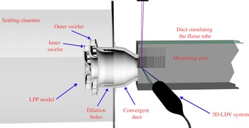
Experimental set-up, 3D-LDV (laser Doppler velocimeter) system and measuring domain.

2.1. Experimental set-up
The large-scale combustor model employed (5:1) is a co-rotating double-swirler centripetal injector (figure 1). It is composed of two swirlers with radial blunt vanes. The internal swirler has 21 blades with an exit angle of
 $40^{\circ }$
with respect to the radial direction, and the external one has 25 blades with an exit angle of
 $53^{\circ }$
. The mean diameters are 102 and 132.3 mm respectively. The mixing tube outlet diameter (
 $D$
) is 104 mm. Downstream of the swirlers a series of radial dilution holes is present. The design swirl number is 0.5 based on the definition given by Pruvost et al. (Reference Pruvost, Legrand, Legentilhomme and Doubliez2000):
 $$\begin{eqnarray}\boldsymbol{S}=\left[\int _{0}^{D/2}u_{x}u_{{\it\theta}}r^{2}\text{d}r\right]\!\left/\left[D/2\int _{0}^{D/2}u_{x}^{2}r\text{d}r\right]\right.,\end{eqnarray}$$
where the generic velocity vector
 $u$
is expressed in cylindrical coordinates (
 $x,r,{\it\theta}$
, indicate the axial, radial and tangential direction respectively).
The mass flow rate is split according to the effective areas of the swirlers: 44 % through the internal swirler, 46 % through the external one and 10 % through the holes.
The test rig (figure 1) consists of a continuous operating wind tunnel of blowdown type. The LPP model is inserted between the settling chamber and a square section duct simulating the flame tube. The latter is 750 mm long and has a cross-section of
 $250~\text{mm}\times 250~\text{mm}$
with optical access from three sides. According to Billant et al. (Reference Billant, Chomaz and Huerre1998), the forms of vortex breakdown and their topology do not seem to be very sensitive to confinement effects when the confinement ratio (the ratio between the exit section diameter/side length and the swirler outlet diameter) is sufficiently large, as in the present experiment. Hence, it may be assumed that the present results have a general validity. The experiments aimed to study the aerodynamic phenomena only. Thus, they have been carried out with isothermal flow. Furthermore, the real operating conditions have been scaled down to atmospheric conditions using the Reynolds similarity only. The selected Reynolds number (
 $\mathit{Re}_{D}$
) equals 260 000 and is based on
 $D$
and the bulk velocity
 $u_{b}=38~\text{m}~\text{s}^{-1}$
. The pressure drop through the LPP model is equal to 2.2 %. The tests have been performed at ambient temperature (298 K).
The measuring domain is composed of 25 radial traverses from
 $x/D=0$
to
 $x/D=1.29$
. Each traverse is defined by 40 points in the range
 $r/D=0$
up to
 $r/D=1$
.
2.2. Measuring systems and preliminary measurements
The three velocity components have been measured by means of a six-beam three-colour fibre optic LDV system operating in backscatter collection mode (Dantec Fiber Flow). The LDV set-up is obtained by combining a 2D and a 1D optical probe, both with 310 mm focal length. The typical measuring volume dimensions are
 $90~{\rm\mu}\text{m}$
diameter and 1.9 mm length. In order to evaluate the time-resolved and spectral characteristics of the flow field, a preliminary set of measurements has been performed by means of a pair of single-sensor hot-wire probes connected to a constant-temperature anemometer (Canepa et al.
Reference Canepa, Di Martino, Formosa, Ubaldi and Zunino2006). For the spectral analysis one hot-wire probe has been radially traversed at several axial locations inside the measuring domain. The results indicate the presence of a periodic flow pattern characterized by a clearly distinct frequency at about 220 Hz. The corresponding Strouhal number
 $St_{D}=fD/u_{b}$
is 0.58, where
 $f$
represents the frequency value. The same frequency peak has been observed in all the investigated axial traverses and for most of the radial locations with similar energy values. The only exceptions are the regions close to the duct axis, where the energy peak attenuates, and the regions outside the swirling flow, where the peak is nearly completely suppressed. Such an analysis has been repeated for
 $\mathit{Re}_{D}$
ranging from 50 000 up to 450 000 and the results indicate that
 $\mathit{St}_{D}$
remains nearly constant within the whole
 $\mathit{Re}_{D}$
range. To have a better insight into the time and spatial flow field characteristics, the two hot-wire probes have been displaced in the axial direction and in the circumferential one. Signals from the two probes have been sampled simultaneously and the fluctuating parts have been both auto- and cross-correlated in time. The autocorrelations show that the periodicity is conserved for a large radial extension, while in the inner region of the swirling jet it is attenuated and in the outer region it is nearly lost. In most of the investigated area the autocorrelation peak for
 $t=0$
is comparable with the amplitude of the periodic oscillation. This indicates that the periodic content is relevant compared with the stochastic part of the signal. From the analysis of the cross-correlation it is possible to evaluate the oscillation period
 ${\it\tau}=0.0045~\text{s}$
, which is independent of the spatial location.
The results show that the propagation speed in the axial direction is about one half of the bulk axial velocity at the LPP model outlet section. These findings are consistent with other works about swirling flows, see for instance Chao et al. (Reference Chao, Leu, Hung and Lin1991) and Panda & McLaughlin (Reference Panda and McLaughlin1994). Thus, the results indicate that the periodic flow perturbation propagates circumferentially at constant rotational speed and this characteristic is present in the whole investigated domain. The rotational speed is equal to
 ${\it\omega}=2{\rm\pi}/0.0045=1382~\text{rad}~\text{s}^{-1}$
. This velocity perturbation, which has been identified as a spiral vortex breakdown (Canepa et al.
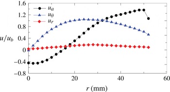
Reference Canepa, Di Martino, Formosa, Ubaldi and Zunino2006), may be studied through the velocity field reconstruction operated by means of phase-locked velocity distributions based on a common phase reference signal. In other words, the periodic flow field is characterized by a rigid-body rotation, and hence the phase-locked measurements performed in the meridional plane are sufficient to reconstruct the flow field within a time period and in a cylindrical space. For the sake of completeness, the profiles of all the three velocity components, made non-dimensional by means of
 $u_{b}$
, are reported in figure 2 (
 $a,r,{\it\theta}$
, indicate the axial, radial and tangential direction respectively).
Radial distributions of the three velocity components at the combustor model outlet.

3. Laser Doppler velocimeter data processing
By means of a single-sensor hot-wire probe located in the flow field, a reference TTL signal (transistor–transistor logic signal) necessary for the ensemble averaging technique has been generated. A total number of 120 000 instantaneous velocity samples for each velocity component has been acquired. The samples have been sorted into
 $N=30$
phase bins, resulting in approximately 4000 samples per bin. Each bin represents a particular phase of the cycle, and the duration of each cycle has been computed by means of the TTL signal. The velocity triple decomposition scheme proposed by Hussain & Reynolds (Reference Hussain and Reynolds1970) for the study of coherent structures in shear flows has been applied. The spectral analysis and the results of the two-point correlations, reported in Canepa et al. (Reference Canepa, Di Martino, Formosa, Ubaldi and Zunino2006), do not show any periodic fluctuations at frequencies different from the fundamental of the vortex breakdown. Therefore, the error in evaluating the random fluctuation
 $u^{\prime }$
should be minimized. A comprehensive evaluation of the LDV measurement accuracy may be found in Canepa et al. (Reference Canepa, Di Martino, Formosa, Ubaldi and Zunino2006). However, it is worthwhile to recall that, to assign a sample to a bin, the time position of the sample is referred to its own specific period computed from the TTL signal peaks just before and after the velocity sample arrival time. This avoids the possibility of phase jitter, although no relevant low-frequency modulation has been detected. Any velocity component
 $u$
at any position can be represented as the sum of the time-averaged contribution
 $\bar{u}$
, the fluctuating component due to the periodic motion
 $\tilde{u} -\bar{u}$
and the random fluctuation
 $u^{\prime }$
:
 $$\begin{eqnarray}u=\bar{u}+(\tilde{u} -\bar{u})+u^{\prime }.\end{eqnarray}$$
The periodic velocity component
 $\tilde{u}$
may be evaluated by means of the ensemble average technique according to
 $$\begin{eqnarray}\tilde{u} (n)=\frac{1}{K_{n}}\mathop{\sum }_{k=1}^{K_{n}}u(n,k),\end{eqnarray}$$
where
 $n=1\dots \,N$
is the index related to the time instants (bins) into which the velocity oscillation period is subdivided and
 $k=1\dots \,K_{n}$
is the index related to the samples within the
 $n$
th time bin. For each measuring point, the three ensemble-averaged velocity components and the six ensemble-averaged Reynolds stress components
 $\widetilde{u_{i}^{\prime }u_{j}^{\prime }}$
have been evaluated. The latter have been calculated according to
 $$\begin{eqnarray}\widetilde{u_{i}^{\prime }u_{j}^{\prime }}(n)=\frac{1}{K_{n}}\mathop{\sum }_{k=1}^{K_{n}}[u_{i}(n,k)-\tilde{u_{i}}(n)][u_{j}(n,k)-\tilde{u_{j}}(n)].\end{eqnarray}$$
For the present measurements, where samples are collected in a meridional plane, the periodic velocity component is a function of the axial coordinate
 $x$
, of the radial one
 $r$
and of
 $n$
. Nevertheless, considering the detected solid-body rotation flow field,
 $n$
may be substituted with the tangential coordinate
 ${\it\theta}=2{\rm\pi}n/N$
in a relative coordinate system:
 $$\begin{eqnarray}\tilde{u} =\tilde{u} (x,r,n)=\tilde{u} (x,r,{\it\theta}).\end{eqnarray}$$
The resulting flow field is expressed in the cylindrical coordinates. Then, spatial derivatives which are necessary to evaluate the various contributions to the TKE production term may be computed. This term has been calculated according to
 $$\begin{eqnarray}P=-{\it\rho}\widetilde{u_{i}^{\prime }u_{j}^{\prime }}\partial \tilde{u} _{i}/\partial x_{j}+\frac{1}{x_{1}}(\tilde{u} _{2}{\it\rho}\widetilde{u_{1}^{\prime }u_{2}^{\prime }}-\tilde{u} _{1}{\it\rho}\widetilde{u_{2}^{\prime 2}}),\end{eqnarray}$$
where
 $x_{1}=r$
,
 $x_{2}={\it\theta}$
,
 $x_{3}=x$
and
 $\partial /\partial x_{1}=\partial /\partial r$
,
 $\partial /\partial x_{2}=(1/r)\partial /\partial {\it\theta}$
,
 $\partial /\partial x_{3}=\partial /\partial x$
;
 $u_{1}=u_{r}$
,
 $u_{2}=u_{{\it\theta}}$
,
 $u_{3}=u_{x}$
.
Equation (3.5) has been derived according to the procedure reported in Tennekes & Lumley (Reference Tennekes and Lumley1972) and employing cylindrical coordinates instead of the Cartesian ones. Shen, Ng & Ni (Reference Shen, Ng and Ni2003) provide the full expression in cylindrical coordinates.
4. Results
4.1. Spatial distribution
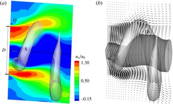
The data are represented in figures 3–6 as 3D isosurfaces together with contour or vector plots in the meridional plane. A light-grey helical-shaped isosurface of constant and positive radial velocity is represented in all the figures (as an indication it is marked as ‘S’ in figure 3 a). It constitutes a reference for the single spiral vortex core. As observed by Canepa et al. (Reference Canepa, Di Martino, Formosa, Ubaldi and Zunino2006), this latter structure rotates in the same direction as the time-mean swirl motion and is counterwinding.
Positive isosurface of
 $\tilde{u} _{r}$
plus (a)
 $\tilde{u} _{x}/u_{b}$
distribution on the meridional plane and (b) vector plot of the velocity on the meridional plane and null
 $\tilde{u} _{x}$
isosurface.

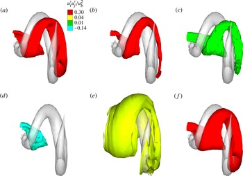
Reynolds stress term isosurfaces: (a) maximum value of
 $\widetilde{u_{x}^{\prime 2}}/u_{b}^{2}$
; (b) maximum value of
 $\widetilde{u_{r}^{\prime 2}}/u_{b}^{2}$
; (c) maximum value of
 $\widetilde{u_{{\it\theta}}^{\prime 2}}/u_{b}^{2}$
; (d) minimum value of
 $\widetilde{u_{x}^{\prime }u_{r}^{\prime }}/u_{b}^{2}$
; (e) maximum value of
 $\widetilde{u_{x}^{\prime }u_{r}^{\prime }}/u_{b}^{2}$
; ( f) maximum value of
 $\text{TKE}/u_{b}^{2}$
.

Turbulent kinetic energy production rate, positive and negative value isosurfaces and meridional contour plot (a–c respectively). (Colour scale:
 $\text{red}=35u_{b}^{3}/D$
,
 $\text{blue}=-35u_{b}^{3}/D$
.)

Turbulent kinetic energy production terms, positive and negative value isosurfaces and meridional contour plot: (a)–(c)
 $({\it\rho}\widetilde{u_{x}^{\prime 2}}\partial \tilde{u} _{x}/\partial x)/(u_{b}^{3}/D)$
; (d)–( f)
 $({\it\rho}\widetilde{u_{r}^{\prime 2}}\partial \tilde{u} _{r}/\partial r)/(u_{b}^{3}/D)$
; (g)–(i)
 $({\it\rho}\widetilde{u_{x}^{\prime }u_{r}^{\prime }}\partial \tilde{u} _{r}/\partial x)/(u_{b}^{3}/D)$
. (Colour scale:
 $\text{red}=35u_{b}^{3}/D$
,
 $\text{green}=-3.5u_{b}^{3}/D$
,
 $\text{blue}=-35u_{b}^{3}/D$
.)

4.1.1. Velocity components
The largest axial velocity (figure 3
a) is observed near the outer radius of the converging nozzle of the premixing duct. These high-axial-velocity spots appear in the upper and lower parts of the duct, and are axially shifted because of the spiralling motion. The centre of the swirling jet is characterized by a large region of negative axial velocity. This recirculation zone is not axisymmetric and its deformation is in phase with the structures in the outer flow. Indeed, it is locally enlarged where it superimposes to the isosurface at positive radial velocity (in light grey). These results agree very well with the results of Oberleithner et al. (Reference Oberleithner, Sieber, Nayeri, Paschereit, Petz, Hege, Noack and Wygnanski2011), who observed that the recirculation region meanders around the duct axis. This zone is characterized by an upstream stagnation point displaced out of the duct axis and rotating about it. This determines a precessing motion, e.g. Brücker (Reference Brücker1993) and Billant et al. (Reference Billant, Chomaz and Huerre1998). This feature is present in the whole vortex breakdown structure and particularly in the vortex core which wraps as a spiral around the separated flow. Hence, this spiral vortex core develops at the border between the inner reverse flow zone and the flow moving downstream. Its intersection with the meridional plane is identified by the presence of two large vortices rotating in the counterclockwise and clockwise directions in the lower and upper portions of the plane respectively. These vortical structures may be appreciated in the vectorial representation of figure 3(b), where they are marked as ‘1A’ and ‘1B’, together with the null
 $\tilde{u_{x}}$
dark-grey isosurface. For simplicity of representation, only the velocity components on the meridional plane are represented. These eddies determine a local outward radial displacement of the separated bubble contour downstream of the isosurface. They give rise to the observed radial oscillations of the separated region and, consequently, also of the surrounding downstream moving flow. Compared with the spiral vortex, the radial velocity isosurface results are slightly shifted in the upstream axial direction. As observed by Brücker (Reference Brücker1993) and Ruith et al. (Reference Ruith, Chen, Meiburg and Maxworthy2003), this process can be related to a mechanism of mass displacement. Indeed, according to the sign of the circumferential vorticity of the eddies, the bubble is filled from its downstream end and it empties from its upstream part. Such vortices at the shear layer boundary seem to be related to an instability mechanism and have a pattern similar to the one observed by Billant et al. (Reference Billant, Chomaz and Huerre1998). Namely, the analysis of the TKE production, reported in § 4.2, will show some analogies with the KH instability. The following discussion will help to identify the physical mechanisms behind the generation of these vortical structures.
4.1.2. Reynolds stresses
The analysis of the six terms of the Reynolds stress tensor has shown that the largest contributions are due to
 $\widetilde{u_{x}^{\prime 2}}$
,
 $\widetilde{u_{r}^{\prime 2}}$
and
 $\widetilde{u_{x}^{\prime }u_{r}^{\prime }}$
, while the other three terms have a lower (negligible) value. The distributions of
 $\widetilde{u_{x}^{\prime 2}}$
,
 $\widetilde{u_{r}^{\prime 2}}$
,
 $\widetilde{u_{{\it\theta}}^{\prime 2}}$
and
 $\widetilde{u_{x}^{\prime }u_{r}^{\prime }}$
, made non-dimensional by means of
 $u_{b}^{2}$
, are depicted in figure 4 as isosurfaces together with the
 $\tilde{u_{r}}$
isosurface. They represent the maximum value of the selected quantity, but for
 $\widetilde{u_{x}^{\prime }u_{r}^{\prime }}$
also the minimum negative value is reported. Colours represent the magnitude. The term
 $\widetilde{u_{{\it\theta}}^{\prime 2}}$
is reported since it provides a contribution to the TKE production near the swirler axis, while
 $\widetilde{u_{x}^{\prime }u_{{\it\theta}}^{\prime }}$
and
 $\widetilde{u_{{\it\theta}}^{\prime }u_{r}^{\prime }}$
are omitted for the sake of space, since they do not provide any significant contribution in (3.5). Moreover, the maximum-value isosurface of the TKE is reported.
The terms
 $\widetilde{u_{x}^{\prime 2}}$
and
 $\widetilde{u_{r}^{\prime 2}}$
indicate that the largest turbulent fluctuations take place at the interface between the reverse flow zone and the spiral vortex core (slightly downstream of the grey isosurface). According to the colour of the isosurface, these two quantities are comparable, but within the remainder of the measurement domain
 $\widetilde{u_{x}^{\prime 2}}$
has a slightly higher intensity than
 $\widetilde{u_{r}^{\prime 2}}$
. All this indicates that the turbulent fluctuations are clearly related to the spiralling motion of the vortex breakdown helix. Indeed, they occur in the downstream inner border of the helix, where large azimuthal vorticity takes place, figure 3(b). This is a first difference from the KH instability that occurs for parallel non-swirling flow characterized by a shear layer in the streamwise direction. Indeed, in the present case, turbulence is not directly linked only to a shear layer of the streamwise velocity. Furthermore, when the KH instability occurs, the turbulent activity of the normal velocity component (the radial one in this case) is typically negligible compared with the streamwise one (see Qadri et al. (Reference Qadri, Mistry and Juniper2013) or the vast literature on laminar separation bubbles developing on airfoils subjected to adverse pressure gradients).
The only non-negligible shear component of the Reynolds stresses is
 $\widetilde{u_{x}^{\prime }u_{r}^{\prime }}$
, which represents the turbulent axial momentum transfer in the radial direction. Namely, it represents the turbulent activity that tends to make the axial (or radial) flow distribution uniform. At negative values (light-blue surface in figure 4
d), the isosurface of
 $\widetilde{u_{x}^{\prime }u_{r}^{\prime }}$
indicates that stochastic velocity fluctuations point inwards (towards the swirler axis) and downstream or outwards and upstream. Hence, they counterbalance the deterministic helix motion which has positive radial velocity. The opposite effect occurs when
 $\widetilde{u_{x}^{\prime }u_{r}^{\prime }}$
is positive (yellow isosurface), as in the outer boundary between the swirling flow and the external nearly quiescent flow, indicated as ‘O’ in figure 3(a) (it has to be remembered that the magnitude of this positive contour level is below half of the negative one depicted in light blue).
4.2. Turbulent kinetic energy production terms
As discussed in § 3, the LDV data have been further postprocessed, according to (3.5), in order to obtain the terms contributing to the TKE production term
 $P$
. Each contribution to
 $P$
accounts for kinetic energy exchanges between mean flow and turbulence. Generally, a positive
 $P$
value results, thus transferring energy to turbulence. Conversely, if
 $P$
is negative, energy is transferred in the opposite direction (Tennekes & Lumley Reference Tennekes and Lumley1972). Here,
 $P$
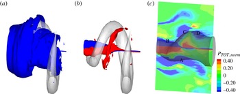
has been computed as the sum of the terms of (3.5) and it is represented in figure 5. In order to highlight the regions inside and outside the one where the vortex breakdown takes place, two isosurfaces are reported in figures 5(a) and 5(b) respectively. The contour plot of
 $P$
in the meridional plane is also reported in figure 5(c). As a result, terms with negative values, e.g. blue isosurfaces, increase the TKE, while positive ones decrease it, e.g. red isosurfaces. The analysis of
 $P$
indicates that the largest contributions are localized in two regions: one is at the interface between the reverse flow zone and the jet, and the other one is located across the shear layer at the outer boundary of the swirling flow. However,
 $P$
attains non-null values also within the region of negative axial velocity about the swirler axis. This area has been highlighted by means of the isosurfaces shown in figure 5(b) and is characterized by two zones of negative and positive values wrapping around the axis. In these zones, the terms
 $1/r\tilde{u} _{r}{\it\rho}\widetilde{u_{{\it\theta}}^{\prime 2}}$
and
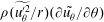 ${\it\rho}(\widetilde{u_{{\it\theta}}^{\prime 2}}/r)(\partial \tilde{u_{{\it\theta}}}/\partial {\it\theta})$
of (3.5) are responsible for the TKE production. They have a nearly symmetric shape with respect to the swirler axis, and the absolute values of
 $P$
are comparable. This particular shape may be explained by considering the distribution of the
 $\tilde{u} _{r}$
and
 $\tilde{u} _{{\it\theta}}$
components caused by the precessing vortex core. Indeed,
 $\tilde{u} _{r}$
is not null about the swirler axis and changes its sign through it. As a consequence, the term
 $1/r\tilde{u} _{r}{\it\rho}\widetilde{u_{{\it\theta}}^{\prime 2}}$
attains values of opposite sign on the two sides of the axis. Similarly, the precessing vortex core leads to change in sign of
 $\partial \tilde{u_{{\it\theta}}}/\partial {\it\theta}$
through the swirler axis. The term
 $\widetilde{u_{{\it\theta}}^{\prime 2}}$
is always positive. As a result, the term
 ${\it\rho}(\widetilde{u_{{\it\theta}}^{\prime 2}}/r)(\partial \tilde{u_{{\it\theta}}}/\partial {\it\theta})$
also changes its sign through the axis.
Summarizing, the TKE production in the region close to the swirler axis has to be ascribed to the terms related to the
 ${\it\theta}$
–
 ${\it\theta}$
normal stress action. This is a preferential zone for the activity of a centrifugal instability mechanism, e.g. Qadri et al. (Reference Qadri, Mistry and Juniper2013). However, this mechanism has an effect on a region of limited extension across the axis, and, most of all, its overall effect is neutral since the production and destruction of TKE compensate. In contrast, the four outer regions marked as ‘A’, ‘B’, ‘C’ and ‘D’ in figure 5(c) identify regions where the TKE is produced. The interpretation of the physical mechanism leading to the TKE production will be discussed in the following, while analysing the single production terms.
The relevant contributions to the TKE production are
 ${\it\rho}\widetilde{u_{x}^{\prime 2}}\partial \tilde{u_{x}}/\partial x$
,
 ${\it\rho}\widetilde{u_{x}^{\prime }u_{r}^{\prime }}\partial \tilde{u_{r}}/\partial x$
along the
 $x$
direction (related to
 $\widetilde{u_{x}^{\prime 2}}$
and
 $\widetilde{u_{x}^{\prime }u_{r}^{\prime }}$
respectively) and
 ${\it\rho}\widetilde{u_{r}^{\prime 2}}\partial \tilde{u_{r}}/\partial r$
along the
 $r$
direction (related to
 $\widetilde{u_{r}^{\prime 2}}$
). They provide by far the largest contribution to the TKE. These terms, made non-dimensional with
 $u_{b}^{3}/D$
, are represented in figure 6 as isosurfaces and contour plots. Three sets of these representations are provided to highlight wherever these terms are negative (figure 6
a,d,g, blue isosurfaces) and increase the TKE, or positive (figure 6
b,e,h, red isosurfaces) and decrease the TKE. For the sake of brevity, the aforementioned production terms will be indicated as
 $P_{xx}$
,
 $P_{rx}$
and
 $P_{rr}$
respectively.
The three terms show their minima at the border between the reverse flow zone and the grey isosurface, which means slightly upstream of the vortex core. This is similar to what has been observed for
 $\widetilde{u_{x}^{\prime 2}}$
,
 $\widetilde{u_{r}^{\prime 2}}$
and
 $\widetilde{u_{x}^{\prime }u_{r}^{\prime }}$
in figure 4. However, compared with the respective Reynolds stress components, the maxima of the absolute values of
 $P_{xx}$
,
 $P_{rx}$
and
 $P_{rr}$
are upstream shifted in the axial direction. This is because the local gradient of the velocity components plays an important role in the determination of the TKE production. Similarly, as already observed, the Reynolds stresses are relevant downstream of their generating cause. In particular,
 $P_{xx}$
generates turbulence in the whole length of the measurement domain, because of the large value of
 $\partial \tilde{u_{x}}/\partial x$
, caused by the spiralling motion. In contrast, the magnitudes of the terms
 $P_{rx}$
and
 $P_{rr}$
become rapidly lower along the axial direction.
The terms
 $P_{rx}$
and
 $P_{rr}$
characterize the production of TKE in a second region of the measurement domain, namely at the outer boundaries of the swirling flow. In this area the turbulence production is mainly due to a large localized velocity gradient: the swirling flow is forced to exchange momentum with the outer almost stagnating fluid. As a consequence, there is a high shear of velocity along the radial direction. This leads to high values of
 $\partial \tilde{u_{r}}/\partial r$
and
 $\partial \tilde{u_{x}}/\partial r$
, and a high
 $\widetilde{u_{x}^{\prime }u_{r}^{\prime }}$
(as previously discussed).
According to Qadri et al. (Reference Qadri, Mistry and Juniper2013), this
 $x$
–
 $r$
shear is a preferential zone for the activity of the KH-like mechanism. Furthermore, the computed production terms are comparable with the production terms measured by Simoni, Ubaldi & Zunino (Reference Simoni, Ubaldi and Zunino2012) in a laminar separation bubble developing over an airfoil with an adverse pressure gradient. In that case, the KH mechanism is driving the transition at the outer shear layer of the separation bubble. The KH instability, for that case, leads to negative values of the terms analogous to
 $P_{rx}$
and positive values of
 $P_{xx}$
(with lower intensity). This is in good agreement with the distribution of
 $P_{rx}$
and
 $P_{xx}$
(red isosurface or bottom isocontour plots) in the outer region. Hence, the turbulent activity in the outer region of the swirling flow seems to be caused by the KH-like instability.
The meridional contour plots of
 $P_{xx}$
,
 $P_{rr}$
and
 $P_{rx}$
are provided in figure 6(c,f,i) together with the isosurface of null axial velocity (dark grey). The figures identify the region at high-turbulence-generation rate in the neighbourhood of the separated region. As an example, the bottom area marked with ‘A’ identifies a shear layer characterized by negative values of
 $P_{rr}$
and
 $P_{rx}$
, and a positive value of
 $P_{xx}$
. Although the flow in this region accelerates along the axial direction,
 $P_{rr}$
and
 $P_{rx}$
prevail on
 $P_{xx}$
leading, overall, to the generation of turbulence. Hence, also in this case, along the spiralling flow region the turbulent activity seems to be continuously generated by a KH-like instability process.
Two further regions (‘B’ and ‘C’) are marked in the plots. The region ‘B’ is characterized by an almost null turbulence production (the intensities of
 $P_{rr}$
and
 $P_{rx}$
are similar but they have opposite sign and
 $P_{xx}$
is negligible). On the contrary, the region ‘C’ shows large values of
 $P_{xx}$
because of the flow deceleration along the axial direction and nearly negligible
 $P_{rr}$
and
 $P_{rx}$
. As a result, in this region, the TKE is expected to increase but the generation mechanism may not be ascribed to KH-like instability. Finally, in the region marked as ‘D’, the distributions of
 $P_{xx}$
,
 $P_{rr}$
and
 $P_{rx}$
are similar to the ones in region ‘A’, and hence they are consistent with the KH mechanism. As a consequence, the shear layer along the recirculation bubble border is somehow correlated to the increase of the TKE. On the contrary, the TKE production seems to be correlated to a KH-like instability only in the region between the bubble and the spiral vortex core (around the light-grey isosurface of the positive radial velocity), since the shear layer shape is consistent with the KH instability. As stated, based on the order-of-magnitude analysis, the generation of turbulent motions is in the main not influenced by the fluctuations of the tangential velocity components and the shear action in the tangential direction, except for a limited region close to the duct axis.
5. Conclusions
In the present paper, an existing database of ensemble-averaged velocity and Reynolds stress downstream of a lean premixing prevaporized burner has been further analysed. The identified solid-body rotation has allowed reconstruction of the periodic flow field in a relative cylindrical frame of reference. The velocity distributions show that a spiral vortex core wraps around an inner reverse flow zone. Both are characterized by a precessing motion. The most important Reynolds stress components are the ones lying in the meridional plane. The maxima of the normal components are located at the border between the separated flow and the spiral vortex core, hence indicating that the turbulent fluctuations are strongly related to the presence of the spiral vortex. The TKE production has been calculated, showing that the only relevant contributions to it are the ones related to the non-negligible Reynolds stress components. Even for these quantities, the maxima are located at the interface between the reverse flow zone and the spiral vortex but, compared with the respective Reynolds stress component, they are axially shifted in the upstream direction due to the local velocity gradient. The production of TKE in the external boundary of the swirling flow is characterized by production term distributions that are consistent with the presence of a Kelvin–Helmholtz-like instability. The analysis of the various contributions to the TKE production on the recirculation bubble boundary suggests that the TKE production seems to be related to a Kelvin–Helmholtz-like instability only in the zones of interface between the bubble and the spiral vortex core. As a consequence, it seems that the vortex core is synchronized with a helical Kelvin–Helmholtz-like instability.