1. INTRODUCTION
One of the most important points concerning navigation safety is to keep the ship on track. Therefore the accuracy of the heading is essential in navigation but, what heading? To clarify the terminology concerning the heading which is expressed from different reference directions, it should be noted that true and magnetic headings are expressed respectively from the true and magnetic meridians, and magnetic compass heading refers to the heading coming from the magnetic compass (Bowditch, Reference Bowditch2002).
Nowadays, most autopilots are capable of receiving at least two headings from different apparatus, one of them is primary and the other secondary. The marine devices giving the heading to the autopilot should be accurate enough to avoid the ship being diverted from her planned track. The two main bridge systems providing an estimated true heading to the autopilot are the gyrocompass and the satellite compass. The gyrocompass performance standards require a minimum deviation from the true heading, always depending on the latitude where the ship is sailing (IMO, 1979; 1995). On the other hand, the satellite compass is a relatively new solution to input the course to an autopilot with a heading accuracy of around 0·5° RMS when operated under the American Wide Area Augmentation System (WAAS) and Differential Global Positioning System (DGPS) (Furuno USA, 2015). Global use of both devices may result in a more accurate value of the true heading input and avoid at the same time the over-reliance on a single electronic navigational aid. Nevertheless, the heading signal from a magnetic compass is often input to the autopilot since the malfunction or switch off of either gyro or satellite compass due to an electrical or system failure would make it impossible for the ship to follow her track automatically. In fact, some autopilots add an alarm when significant alterations between the heading coming from primary and secondary sources appear.
The only means to provide the Officer of the Watch (OOW) with a valid heading at all times is the magnetic compass. For this reason, IMO (2014) lays down in paragraphs 2.1.1, 2.1.2, 2.1.3 and 2.2.1 of Chapter V, Regulation 19 of the Safety of Lives at Sea (SOLAS) Convention the requirements for merchant ships to be fitted with a magnetic compass to determine and display the vessel's heading independent of any power supply together with a means for correcting heading and bearings to true at all times. Therefore officers on watch have to monitor true course from the magnetic compass using scientific methods (Lushnikov, Reference Lushnikov2012). The total magnetic compass error is the algebraic sum of the magnetic variation that is caused by the Earth's internal magnetism, and the deviation, which is caused by the magnetic material of which the ship is built. The magnetic variation and the horizontal and vertical components of the Earth's field may be easily calculated by means of the geomagnetic models once the time, observer height and estimated ship position are known (Zmuda, Reference Zmuda1971). Nevertheless, it is important to point out that the algorithm of this model does not allow for magnetic storms and local magnetic anomalies such as, for instance, those anomalies caused by the ferromagnetic objects of some sea areas (Woloszyn, Reference Woloszyn2008). On the other hand, the deviation is different for each course the ship is steering and for each geographical position of the ship. Therefore, a process of compass compensation should be carried out at different positions to reduce the deviation to residual values. Moreover, the deviation differs over time and compass compensation must be performed at least every two years (one year according to some regulations) and every time that the ship magnetism changes suddenly (ISO, 2009). Some thoughts and experiences concerning violent changes in ship magnetism, such as lightning striking metallic installations of the ship, are related by Kemp (Reference Kemp2010).
The method to compensate the magnetic compass, called compass adjustment, has remained invariable for more than a century and requires the ship to leave the berth to execute a complete swing circulation (Jenkins, Reference Jenkins1869). This means an extra cost for the ship owner and, perhaps more important, an increase in port traffic affecting port safety. In this respect and, based on a specific adjuster service report provided by the master of the 150,000 deadweight tonne crude oil tanker on which the experiment was carried out, the time elapsed to carry out the adjustment for this type of ship in Rotterdam port was around three hours which means that the fuel, port expenses and running costs may add up to more than 6,000 Euros.
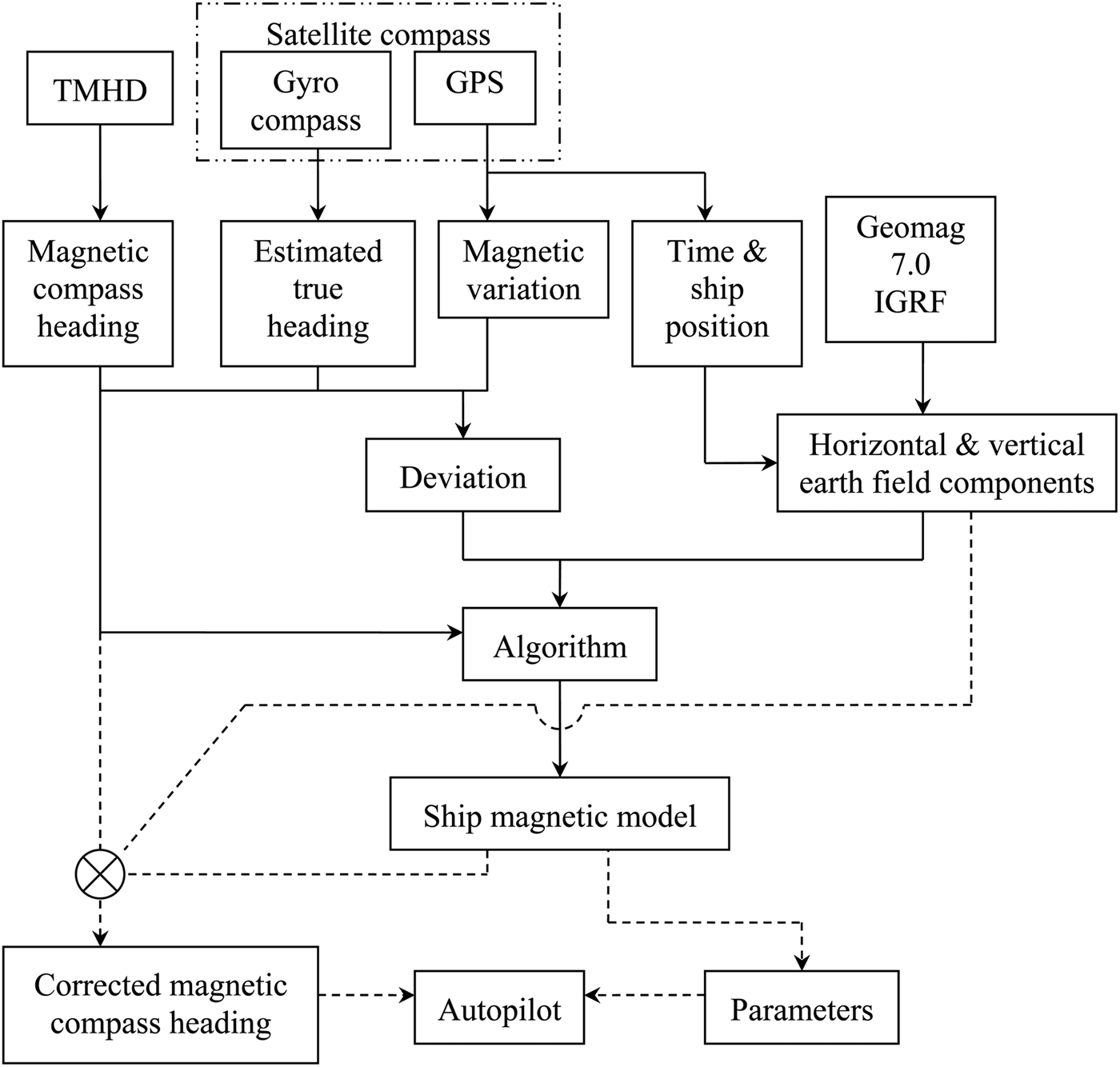
The aim of this paper is to create a ship magnetic model with a double purpose: firstly to correct the magnetic compass heading input to the autopilot and, secondly to provide enough information to carry out the compass compensation without moving the ship. The structure of the system, shown in Figure 1, is based on an algorithm that needs to be fed by heading from gyro and/or satellite compass, magnetic compass heading, position and time. The communication between these devices is based on the National Marine Electronics Association (NMEA) protocol (Martinez et al., Reference Martínez, Vila, Piniella and Martinez2008). Therefore, the system will need a Transmitting Magnetic Heading Device (TMHD) for generating a suitable output signal of magnetic compass heading for the autopilot according to IMO regulations (IMO, 1998; 2000). It is important to note that the system considers the gyrocompass heading or the satellite compass heading, or a global heading obtained from both, as the true heading in order to calculate, by the subtraction of magnetic compass heading and true heading, the total magnetic compass error. The algorithm can easily run into the autopilot software correcting the magnetic compass heading and providing the ship magnetic model in a display. The data collected from other devices includes magnetic compass heading, gyro and/or satellite compass heading, magnetic variation, position, date and time. Alterations in data due to malfunction of these devices may be detected and data collection stopped. The horizontal and vertical components of magnetic earth field can be obtained by means of the free Geomag 7.0 software (IAGA, 2014). This program is based on the IGRF 11th generation geomagnetic model which is valid up to 2015 (Finlay et al., Reference Finlay, Maus, Beggan, Bondar, Chambodut, Chernova, Chulliat, Golovkov, Hamilton, Hamoudi, Holme, Hulot, Kuang, Langlais, Lesur, Lowes, Lühr, Macmillan, Mandea, McLean, Manoj, Menvielle, Michaelis, Olsen, Rauberg, Rother, Sabaka, Tangborn, Tøffner-Clausen, Thébault, Thomson, Wardinski, Wei and Zvereva2010). For geomagnetic data beyond 2015, the website of the National Geophysical Data Center belonging to the U.S. National Oceanic and Atmospheric Administration provides a new world magnetic model developed jointly with the British Geological Survey (NOAA, 2015). Once the magnetic variation and the total magnetic compass error are known, the deviation is easily calculated by subtraction of both. The necessary input data consists of the magnetic compass heading, deviation and horizontal and vertical earth field components which, once stored for at least twenty-four equidistant headings (around 15° each), are processed by the algorithm providing us with the ship magnetic model for a point positioned at the centre of the compass card. It is important to note that the data stored should be collected at different ship positions with high changes in latitude so that the magnetic model parameters related to the vertical soft irons may be calculated accordingly (Basterretxea et al., Reference Basterretxea, Vila and Perez Labajos2014). In this way, the geographic variability of the magnetic deviation may be corrected. Moreover, data collection should be limited to a short period of time because of the temporary alterations to the ship's magnetism. On the other hand, the data has to be filtered to eliminate orthogonality error between the horizontal and vertical planes. Related to this, the magnetic compass heading is unstable when the ship is rolling or yawing hard and the system may stop data collection when this happens. In the same way, no data should be collected when the ship is loaded with steel products or other magnetic cargo or even when it is berthed near metallic port installations.
System structure.

The ship magnetic model consists of the two horizontal components of the permanent magnetism and the coefficients of the horizontal tensors of susceptibility of the transient magnetism in fore-and-aft and athwart axes. The first ones are expressed in the same unit as the earth field components (normally in gauss or nanoteslas) and the second ones are dimensionless. All these parameters are expressed as a function of the shielding factor which is the ratio between two magnetic strengths. This factor cannot be calculated by the algorithm because the data provided by the TMHD under the NMEA protocol only includes the heading and not the strength. In the case where we might try to obtain the strength using for instance a three-axis fluxgate magnetometer, the magnetic field would be greatly disturbed by the magnets of the compass card and, consequently, no data might be collected due to saturation. Therefore the only method for finding the shielding factor would consist of removing the compass bowl when the ship was berthed and setting a magnetometer in its place. Taking into account that, nowadays, most tablets or cellular phones come with a magnetometer inside, it would not be difficult for a compass adjuster or ship officer to obtain the field vector.
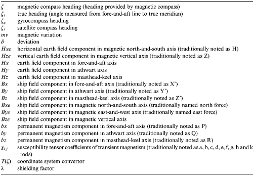
In the following paragraphs, compensation theory and the ship magnetic model algorithm will be discussed. Table 1 provides the nomenclature used in these paragraphs. A simulation will be carried out to compare the pre-arranged ship magnetic model parameters with those estimated by the algorithm. Additionally, the estimated deviation and the corrected magnetic compass heading are evaluated. Finally, all of this is tested on a real ship.
Symbols' meaning.

2. COMPENSATION THEORY AND SHIP MAGNETIC MODEL CALCULATION
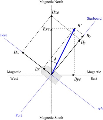
The total magnetic field that affects the magnetic compass on board includes the Earth field and the magnetism created by the ship irons at the position of the needle. The latter is referred to as ship field. Taking into account that ships are floating on the water, their motions are more damped than other vehicles such as aircraft, helicopters, etc. Therefore, if the ship motions, and especially the rolling, are not too exaggerated, the vertical components of the earth and ship magnetism would not affect the deviation and, consequently, the compensation of the magnetic compass may be studied on the basis that the ship is upright. Nevertheless, the heeling error in deviation when the vessel is rolling is the cause of unsteadiness of the compass on north and south headings and, in consequence, the heeling magnet should be set properly in the binnacle (Grant and Klinkert, Reference Grant and Klinkert1970; Klinkert, Reference Klinkert1976). In this way, the non-orthogonality between horizontal axes and Z axis may be considered negligible. In Figure 2 the horizontal component of ship field B’ is decomposed according to two coordinate systems: one formed by fore-and-aft and athwart axes and another one by magnetic north-south and east-west axes.
Ship field components.

The compensation theory applicable to magnetometers is different from that applicable to the magnetic compass on board. Magnetometers are used to measure magnetic field intensity on marine vehicles, whereas the magnetic compass is used to assess the angle between B’ force and the fore-and-aft axis and does not provide magnetic field intensity. Calibration in magnetometers uses methods such as non-linear least squares (Pang et al., Reference Pang, Li, Chen, Pan, Luo, Zhang and Luo2013), differential evolution algorithm (Pang et al., Reference Pang, Zhang, Wang, Wang, Li, Luo, Chen, Pan and Luo2013), relative motion (Auster et al., Reference Auster, Fornacon, Georgescu, Glassmeier and Motschmann2002), or inertial sensors (Koo et al., Reference Koo, Sung and Lee2009), among others, to compensate the effect of hard and soft irons as well as the scale factor, noise, etc. Eddy current field and low frequency magnetic field are also considered in vector compensation methods for magnetometers (Pang et al., Reference Pang, Zhang, Li, Luo, Chen, Pan and Luo2014). However, a magnetic compass does not need to be as accurate as a magnetometer and consequently there are some clear differences on how to compensate both devices. For instance, the scale factor and noise do not exist in the magnetic compass and the effect of eddy currents, known as Gaussian error on board ships, would be considered as negligible three minutes after an appreciable turn of the ship. With regard to the magnetic compass, compensation theory is based on investigations in the 19th century (Barber and Arrot, Reference Barber and Arrott1988) but, contrary to what one might think, do not differ so much from the present compensation methods applicable to magnetometers. Thus, the old equations given by Siméon Denis Poisson in 1824, shown in Equation (1), seem to be near the traditional error model of a three-axis magnetometer (Crassidis et al., Reference Crassidis, Lai and Harman2005). Focusing on the investigations into magnetic compass adjustment, Archibald-Smith and Evans (Reference Archibald-Smith and Evans1863), based on Poisson's equations, produced in the middle of the 19th century the equation of the deviation as a way to calculate and reduce the alterations of the magnetic compass heading caused by the ship's irons. In this way, they gave a first step to establish a method of compensation that is even today applicable on board all ships with satisfactory results.
The development of the algorithm proposed in this paper starts in the original Poisson's equations expressed in Equation (1) which are referred to the fore-and-aft axis. The components may be referred to the magnetic meridian axis using the conversion matrix in Equation (2) (Estevez and Fernandez, Reference Estevez and Fernandez1995). Therefore, Poisson's equations may be expressed as in Equation (3) where the earth components Hxe and Hze may be obtained directly from geomagnetic models.
 $$\left[ {\matrix{ {Bx} \cr {By} \cr {Bz} \cr}} \right] = \left[ {\matrix{ {Hx} \cr {Hy} \cr {Hz} \cr}} \right] + \left[ {\matrix{ {\chi _{1,1}} & {\chi _{1,2}} & {\chi _{1,3}} \cr {\chi _{2,1}} & {\chi _{2,2}} & {\chi _{2,3}} \cr {\chi _{3,1}} & {\chi _{3,2}} & {\chi _{3,3}} \cr}} \right] \cdot \left[ {\matrix{ {Hx} \cr {Hy} \cr {Hz} \cr}} \right] + \left[ {\matrix{ {bx} \cr {by} \cr {bz} \cr}} \right]$$
 $$T(\zeta ) = \left[ {\matrix{ {cos \;\zeta} & { - sin \;\zeta} & 0 \cr {sin \;\zeta} & {cos \;\zeta} & 0 \cr 0 & 0 & 1 \cr}} \right]$$
 $$\left[ {\matrix{ {Bxe} \cr {Bye} \cr {Bze} \cr}} \right] = \left[ {\matrix{ {Hxe} \cr 0 \cr {Hze} \cr}} \right] + T(\zeta ) \cdot \left[ {\matrix{ {\chi _{1,1}} & {\chi _{1,2}} & {\chi _{1,3}} \cr {\chi _{2,1}} & {\chi _{2,2}} & {\chi _{2,3}} \cr {\chi _{3,1}} & {\chi _{3,2}} & {\chi _{3,3}} \cr}} \right] \cdot T^t (\zeta ) \cdot \left[ {\matrix{ {Hx} \cr {Hy} \cr {Hz} \cr}} \right] + T(\zeta ) \cdot \left[ {\matrix{ {bx} \cr {by} \cr {bz} \cr}} \right]$$
The intensity and direction of the horizontal component of ship field B’ and its component in the magnetic meridian Bxe, known as directive force, vary depending on the ship heading and position. The relation (ratio) between the average of the intensities of the directive forces at equidistant headings and the horizontal component of earth field Hxe is expressed by the shielding factor or coefficient lambda λ. Therefore, this factor will depend on the intensity of the ship field that cannot be measured by the TMHD because of the effect on the magnetic field created by the magnets of the compass card, as commented before. The value of the shielding factor may be expressed as a function of susceptibility tensor coefficients as in Equation (4) (Denne, Reference Denne1998).
 $$\lambda = 1 + 0 \!\cdot \!5\cdot\!\left( {\chi _{1,1} + \chi _{2,2}} \right)$$
The deviation may be expressed as a function of Bxe and Bye as in Equation (5). If both components of ship field are substituted by their value in Equation (3), the deviation may be expressed as Equation (6).
 $$tan \;\delta = \displaystyle{{sin \;\delta} \over {cos \;\delta}} = \displaystyle{{Bye} \over {Bxe}}$$
 $$\eqalign{& \lambda \cdot Hxe \cdot sin \;\delta = bx \cdot sin \;\zeta + {\chi _{1,3}} \cdot Hze \cdot sin \;\zeta + by \cdot cos \;\zeta + {\chi _{2,3}} \cdot Hze \cdot cos \;\zeta + \cr & + \displaystyle{{Hxe} \over 2} \cdot \left[ \matrix{\left( {{\chi _{1,1}} - {\chi _{2,2}}} \right) \cdot sin \left( {2\zeta + \delta } \right) + {\chi _{1,2}} \cdot \left\{ {cos \left( {2\zeta + \delta } \right) - cos \;\delta } \right\} \hfill \cr + {\chi _{2,1}} \cdot \left\{ {cos \left( {2\zeta + \delta } \right) + cos \;\delta } \right\} \hfill} \right]} $$
In the latter, the earth field components Hxe and Hze will change with the ship position, the deviation will change with both ship heading and position and the rest of the parameters, including the shielding factor, do not change. Therefore, an overdetermined system of equations may be reached for, preferably, n equidistant headings at different ship positions. Obviously, it would be preferable not to collect data near magnetic poles where compasses are not working correctly (Lushnikov, Reference Lushnikov2009; Thomas, Reference Thomas1951). This equation system may be expressed as in Equation (7) where W is the coefficient matrix, D(δ) the column vector of deviations, H the column vector of the horizontal earth field components in magnetic meridian and M the ship magnetic model, the value being as in Equations (8), (9) and (10).
 $$H \cdot D\left( \delta \right) = M \cdot W$$
 $$\eqalign{ W &= \left[\matrix{ {sin \;\zeta _1} & {Hze_1 \;sin \zeta _1} & {cos \zeta _1} & {Hze_1 cos \zeta _1} & {\displaystyle{{Hxe_1} \over 2}sin (2\zeta _1 + \delta _1 )} \cr {sin \zeta _2} & {Hze_2 \;sin \zeta _2} & {cos \zeta _2} & {Hze_2 cos \zeta _2} & {\displaystyle{{Hxe_2} \over 2}sin (2\zeta _2 + \delta _2 )} \cr \vdots & \vdots &\vdots & \vdots & \vdots & \cr {sin \zeta _n} & {Hze_n \;sin \zeta _n} & {cos \zeta _n} & {Hze_n cos \zeta _n} & {\displaystyle{{Hxe_n} \over 2}sin (2\zeta _n + \delta _n )} \cr} \right. \cr &\left. \matrix{{\displaystyle{{Hxe_1} \over 2}\left[ {cos (2\zeta _1 + \delta _1 ) - cos \delta _1} \right]} &{\displaystyle{{Hxe_1} \over 2}\left[ {cos (2\zeta _1 + \delta _1 ) + cos \delta _1} \right]} \cr {\displaystyle{{Hxe_2} \over 2}\left[ {cos (2\zeta _2 + \delta _2 ) - cos \delta _2} \right]} &{\displaystyle{{Hxe_2} \over 2}\left[ {cos (2\zeta _2 + \delta _2 ) + cos \delta _2} \right]} \cr \vdots & \vdots \cr {\displaystyle{{Hxe_n} \over 2}\left[ {cos (2\zeta _n + \delta _n ) - cos \delta _n} \right]} &\displaystyle{{Hxe_n} \over 2}\left[ {cos (2\zeta _n + \delta _n ) + cos \delta _n} \right]\cr}\right]}$$
 $$H = \left[ {\matrix{ {Hxe_1} \cr {Hxe_2} \cr \vdots \cr {Hxe_n} \cr}} \right] \quad \quad D\left( \delta \right) = \left[ {\matrix{ {sin \;\delta _1} \cr {sin \;\delta _2} \cr \vdots \cr {sin \;\delta _n} \cr}} \right]$$
 $$M^t = \left[ {\matrix{ {bx} & {\chi _{1,3}} & {by} & {\chi _{2,3}} & {\left( {\chi _{1,1} - \chi _{2,2}} \right)} & {\chi _{1,2}} & {\chi _{2,1}} \cr}} \right]$$
The deviation in Equation (9) is obtained by subtraction of the sum of magnetic variation and magnetic compass heading from the heading obtained from gyro and/or satellite compass. In case both sources provide data to the autopilot, a mean value may be calculated by semi-sum or least squares method. Therefore, the only unknowns in Equation (7) are the elements of M or, similarly, the parameters of the ship magnetic model. Their value may be obtained in function of the shielding factor by the algorithm expressed in Equation (11) which is based in the least squares method (Felski, Reference Felski1999; Admiralty Compass Observatory, 1948).
 $${{M} \big / {\lambda}} = \left[ {W^T \cdot W} \right]^{ - 1} \cdot W^T \cdot H \cdot D(\delta )$$
As can be seen in Equation (6), the accuracy in calculating bx, by, χ 1,3 and χ 2,3 will depend on the alteration of Hze or, similarly, on the changes of ship position and especially of latitude (Basterretxea et al., Reference Basterretxea, Vila and Perez Labajos2014). If the ship does not change her position, the components of permanent magnetism (bx and by) could not be separated from the parameters of transient magnetism (χ 1,3 and χ 2,3 ). A known way to obtain these parameters more accurately is to collect data at cardinal headings at different positions with large differences in latitude (NGA, 2004). Theoretically, it would be possible to calculate χ 1,3 separately by heeling the ship, however this method is only valid for a list of over 15°, which is unusual in a ship (Basterretxea et al., Reference Basterretxea, Vila and Sotes2013). It is also important to note that these four parameters are considered the least stable ones (Lushnikov, Reference Lushnikov2010). For this reason, it is very important to make an accurate calculation of these four parameters by collecting, if possible, various cardinal headings from the magnetic compass with a large variation of latitude.
Once the parameters of the ship magnetic model in the function of the shielding factor are known, the deviation for any ship heading and position may be estimated and, in this way, the autopilot may correct the magnetic compass heading accordingly. However, this information would not be enough to compensate the magnetic compass in port without the necessity of moving the ship because it is necessary to know the value of the shielding factor. One method that the compass adjuster can use to calculate this factor consists of taking a measurement of the ship field by means of a magnetometer placed in the centre of the compass card. As mentioned before, it is necessary to remove the compass bowl before taking the measurements of the components Bx and By so that the magnetic element of the card does not affect the measurements. Once the components have been obtained, the first two Poisson's equations may be transformed as in Equation (12) where the coefficients Kx and Ky can be obtained from Equations (13) and (14).
 $$\left[ {\matrix{ {Bx - Kx - Hx} \cr {By - Ky - Hy} \cr}} \right] = \left[ {\matrix{ {\chi _{1,1}} \cr {\chi _{2,2}} \cr}} \right] \cdot \left[ {\matrix{ {Hx + 0\! \cdot \!5 \cdot\!Kx} & {0 \!\cdot \!5 \cdot\!Kx} \cr {0 \!\cdot \!5 \cdot\!Ky} & {Hy + 0 \!\cdot \!5 \cdot\!Ky} \cr}} \right]$$
 $$Kx = {\chi _{1,2} \big / \lambda } \cdot {Hy} + {\chi _{1,3} \big / \lambda } \cdot {Hz} + {bx} \big /{\lambda}$$
 $$Ky = {\chi _{2,1} \big / \lambda } \cdot {Hy} + {\chi _{2,3} \big / \lambda } \cdot {Hz} + {by} \big /{\lambda}$$
Thus, the susceptibility coefficients of transient magnetism necessary to calculate the shielding factor by Equation (4) can be obtained from Equation (12). In this way, the rest of the parameters of the ship magnetic model may be obtained separately from this factor.
3. SIMULATION
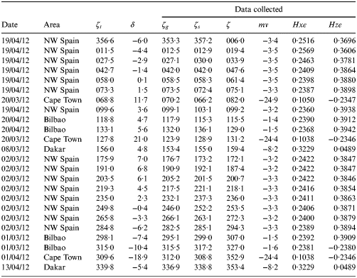
Simulation is carried out to compare pre-arranged data with estimated data obtained by the algorithm taking into account usual compass errors. A hypothetical round-trip voyage from Bilbao (Spain)-Port Elizabeth (South Africa) is assumed from 1 March to 22 April 2012. Magnetic variation and earth field components are obtained for a particular ship position and date by means of the Geomag 7·0 software. Table 2 provides pre-arranged data that the system would collect during the simulated voyage. ζt and ζ denote respectively the true and magnetic compass headings obtained from the pre-arranged deviation δ. ζg and ζs denote respectively the gyrocompass and satellite compass headings selected at random provided that the maximum error is around 4°. Earth components are expressed in gauss.
Simulation data.

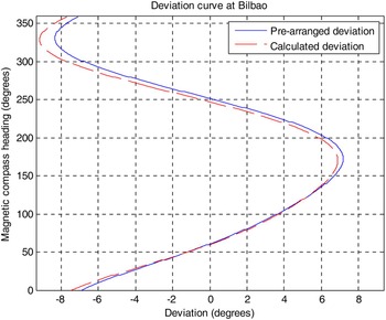
Once the voyage has finished at Bilbao on 22 April 2012, estimated parameters are calculated in function of lambda by the application of Equation (11). Geomagnetic data is also obtained for that place and date. Values of Bx and By at true heading 044·6° are obtained from the pre-arranged parameters to calculate estimated parameters χ 1,1 and χ 2,2 by the application of Equation (12). In this way, the value of lambda calculated by Equation (4) may be separated from the rest of the estimated parameters. Table 3 compares pre-arranged and estimated parameters of the ship magnetic model. As can be seen, the calculation may be considered as good since both data do not differ much. The estimated deviation obtained from the algorithm is also compared to the pre-arranged deviation in Figure 3.
Comparison between pre-arranged and estimated deviation.

Comparison between pre-arranged and calculated parameters.

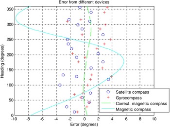
Figure 4 shows the total heading error of the different compasses obtained from the comparison with the true heading. It should be taken into account that for the magnetic compass, factors such as diurnal changes in the variation can amount to 0·2° and atmospheric disturbances or local anomalies can create similar or larger errors. In the same way, acceleration effects, particularly when a ship makes frequent alterations of course while yawing, can cause errors of a similar order in gyro compasses. The corrected magnetic compass heading has been obtained by the algebraic sum of magnetic compass heading, magnetic variation and estimated deviation. As can be seen, this corrected magnetic compass heading seems to be more accurate than headings obtained from gyrocompass or satellite compass. That means that the autopilot running with the corrected magnetic compass may be even more accurate than working with the gyrocompass or satellite compass. As mentioned before, it is not necessary that the algorithm is fed by the exact value of the shielding factor to obtain the corrected magnetic compass heading. However, this factor should be calculated previously in case the ship magnetic model is used to carry out the compass adjustment. This process will be explained further in the experiment carried out on board a Suezmax tanker.
Simulation results of heading errors from different navigation devices at Bilbao on 22 April 2012.

4. EXPERIMENT
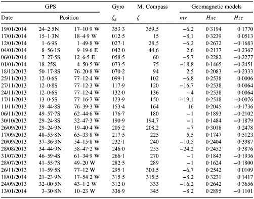
The experiment was carried out on board a Suezmax tanker fitted with a magnetic compass adjusted on 12 October 2012. Appropriate software was installed to collect data from the gyrocompass, TMHD and DGPS receptor using the NMEA protocol. The data were collected in the experiment from 28 July 2013 to 1 February 2014. This collection period should be as short as possible since the ship magnetism may sustain changes over time. Once the ship was berthed at true heading 046·1° in Bilbao on 1 February 2014, the compass bowl was removed and the following values were measured with a magnetometer: Bx 0·166 and By −0·172 gauss. These values of ship field let us determine the parameters χ 1,1 and χ 2,2 by the application of Equation (12). A ship berthed nearly at an inter-cardinal heading is the optimal manner to obtain ship field components as well as to reduce parameters χ 1,1 and χ 2,2 during compass adjustment.
The data selected to run the algorithm are shown in Table 4 where earth components are expressed in gauss. The estimated parameters obtained are shown in Table 5. On the other hand, it should be noted that the software includes filters to stop data collection:
-
■ during around three minutes after an appreciable change of ship heading to avoid Gaussian error, and
-
■ when the heading was too variable (± 2° in less than half minute) due to yawing or rolling.
Data collected from gyrocompass, TMHD and GPS during the experiment.

Ship magnetic model parameters obtained in the experiment.

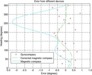
On 1 February 2014 the ship executed a complete swing circulation approaching Bilbao with the results presented in Table 6 which serve to compare the heading error of different devices as shown in Figure 5.
Results of heading errors of different navigation devices on board MV Monte Toledo at Bilbao on 1 February 2014.

Headings obtained during swing circulation execution.

With regard to this, officers were informed previously that the collection process should be re-started in case the ship magnetism was altered suddenly. Equally, software should be stopped manually when the ship was berthed near metallic port installations or loaded with steel products.
With respect to the compass adjustment, parameters in Table 5 had to be reduced by changing the magnetic field generated by the correctors. The components bx and by were affected by the horizontal correctors (fore-and-aft and athwartship magnets respectively) set in the binnacle, the parameters χ 1,1 and χ 2,2 by the boxes (or spheres or cylinders) and χ 1,3 by the Flinders' bar. The rest of the parameters could have been reduced if it had been possible to slew the boxes and the Flinders' bar. That was not the case on this type of ship. On the other hand, it is considered that a little part of the deviation might be caused by a wrong installation of the magnetic compass. In the case of the experiment, this installation was misaligned only 0·05°. The part of the deviation caused by each parameter might be calculated from Equation (7). In this way, the part of deviation caused jointly by χ 1,1 and χ 2,2 at true heading 046·1° was equal to −0·13° and that generated by χ 1,3 was 0·25°.
Compass adjustment is carried out as follows:
-
1. Flinders' bar was set initially to 300 mm length. The part of deviation caused by χ 1,3 was reduced by shortening the bar to 273 mm length. This compensation would not be possible if the ship were berthed at north or south headings.
-
2. Boxes were not altered since the deviation jointly generated by χ 1,1 and χ 2,2 was too low. To reduce this part of deviation, boxes should be moved away from the compass card to move the needle only 0·13°.
-
3. Taking into account the magnetic moment of each horizontal corrector (5·75×10−10 N m in this case), the parameter bx was reduced to −0·0006 by lowering a pair of fore-and-aft magnets red aft from hole 5 to 3 (Arribalzaga et al., Reference Arribalzaga, Martínez and Vila2013). To do this, the field affecting the magnetic compass by the magnets placed in each one of the holes of the binnacle was calculated previously.
-
4. Using the same correctors as before, the parameter by was reduced to 0·0004 by lowering athwart magnet red port from hole 7 to 3.
5. CONCLUSIONS
The ship magnetic model obtained by the algorithm presented in this paper may be used to correct the magnetic compass heading input in the autopilot. The precision of this heading is better than gyrocompass or satellite compass heading as the results of the simulation and experiment verify. Moreover, the corrections are valid for all navigational areas since the alterations in the deviation attributable to the variations of geomagnetic forces are reduced.
On the other hand, the parameters of the ship magnetic model also permit us to carry out a compass adjustment (including the Flinders bar correction) at a single heading and single magnetic latitude. There are other methods to compensate the deviation at a single heading but in an approximate manner (Lushnikov, Reference Lushnikov2011). Nevertheless, it should be noted that accuracy in the method presented in this paper is lost when the ship is berthed near cardinal headings.
FINANCIAL SUPPORT
This work has been performed by the University of the Basque Country within the project “COMPASS”, which has been financed by the Basque Agency for Business Development (SPRI) under the grant number SA-2012/00339.