


I. Introduction
Climate change and its impacts have become the center of debate among policymakers due to the notable increase in the number of natural disasters, particularly weather-related events, over the past several decades. To better understand how climate change affects the overall economy, several studies have explored the potential impact of climate risk on the capital market (e.g., Bernstein, Gustafson, and Lewis (Reference Bernstein, Gustafson and Lewis2019), Bolton and Kacperczyk (Reference Bolton and Kacperczyk2021)). There is also a strand of literature highlighting that severe disasters can lead individuals to overestimate the risk of similar future events and bias their decision-making, a phenomenon known as the salience bias (Bordalo, Gennaioli, and Shleifer (Reference Bordalo, Gennaioli and Shleifer2012)). For example, both corporate managers and professional fund managers are found to respond irrationally to climatic disasters in the short term (Dessaint and Matray (Reference Dessaint and Matray2017), Alok, Kuma, and Wermers (Reference Alok, Kuma and Wermers2020)). Since individuals’ risk beliefs affect their decision-making processes, it is crucial to understand whether and how severe natural disasters affect other important players in the capital market.
In this article, we aim to explore whether bank lenders correctly understand the implications associated with natural disaster risks. Compared with corporate and fund managers, bankers are more concerned about downside risks. As a result, bank lenders may be more responsive to events like natural disasters that could affect their assessment of borrowers’ creditworthiness (Gorton and Kahn (Reference Gorton and Kahn2000)). Bank financing serves as a primary source of capital for firms in the United States. Using a sample of 305 nonfinancial public U.S. firms over the period 1996 to 2006, Rauh and Sufi (Reference Rauh and Sufi2010) show that approximately 68% of these firms use bank debt. Using more comprehensive samples, Colla, Ippolito, and Li (Reference Colla, Ippolito and Li2013) (Reference Colla, Ippolito and Li2020) report that about 50% of nonfinancial firms in the United States use bank debt. Therefore, it is crucial to understand whether bank lenders can accurately estimate the impact of disasters on firms. If bankers are subject to similar salience bias as other professionals, they might allocate credit inefficiently, leading to significant financing costs for corporate firms and ultimately impacting corporate investment. We refer to this as our salience hypothesis.
Bankers typically make corporate lending decisions collectively through loan syndicates, especially when there are multiple lead arrangers. Prior work in behavioral economics and psychology suggests that groups can behave systematically differently from individuals, sometimes mitigating and sometimes amplifying behavioral biases (e.g., Kerr, MacCoun, and Kramer (Reference Kerr, MacCoun and Kramer1996), Charness and Sutter (Reference Charness and Sutter2012)). As a result, it is ex ante unclear whether the salience-driven responses documented for individual decision-makers should also arise in a setting characterized by collective decision-making. Because many important financial decisions are made in groups rather than in isolation, studying how bank lenders respond to severe natural disasters provides insight into whether collective decision-making attenuates or exacerbates the effects of behavioral biases.
To answer these questions, we study bank lenders’ reactions to major disaster events when their borrowers have major operations in the neighborhood of a disaster region. Natural disasters are largely unpredictable. When a natural catastrophe occurs (e.g., hits a region), it does not materially affect the likelihood that a neighboring region will be hit by another disaster in subsequent years (Dessaint and Matray (Reference Dessaint and Matray2017)). By focusing on borrowers that could have been affected by a disaster event but were not because of chance, we are able to assess whether bank lenders can gauge these borrowers’ disaster risk correctly. More specifically, we conjecture that when banks make lending decisions to firms close to the disaster area, they are more susceptible to salience bias and thus more likely to overestimate the risk of similar disasters. If so, such bias would lead to an increase in loan spreads for borrowing firms located in the neighboring region of a disaster.
On the other hand, there are also good reasons that banks might not respond irrationally to severe natural disasters. Banks are widely regarded as sophisticated players in the capital market due to their superb ability to collect and analyze information. Compared with corporate and fund managers, bankers may be less subject to biases and errors in their decision-making. Moreover, observing an increase in loan spreads for neighboring firms following a disaster does not necessarily mean that it is a result of salience bias. It is thus critical for us to design the tests carefully to evaluate alternative explanations.
Using bank loan data from DealScan during the period 1987–2017, we find that about 8% of corporate loans are issued to borrowers having major operations in the neighborhood of a region hit by a natural disaster in the previous 2 years.Footnote 1 More importantly, we find that the loan spreads for these borrowers are 6% (13 basis points) higher than those paid by remote firms, controlling for determinants of loan spreads that include firm and loan characteristics, and various fixed effects that include firm, state-year, bank-year, and industry-year fixed effects. The results are robust when we conduct analysis based on an entropy-balanced sample. These findings are consistent with our salience hypothesis that a sudden shock to perceived disaster risk leads lenders to increase the loan spreads for borrowers with major operations in the neighboring counties of the disaster area.
To better establish causality, we next study the dynamic effects of salient disaster events on neighboring firms’ loan spreads. We find that the increase in loan spreads does not occur prior to the disaster, and the positive impact diminishes within 1 year after the disaster. These patterns support a causal interpretation of our results and align with the note that the effect of salience bias diminishes over time.
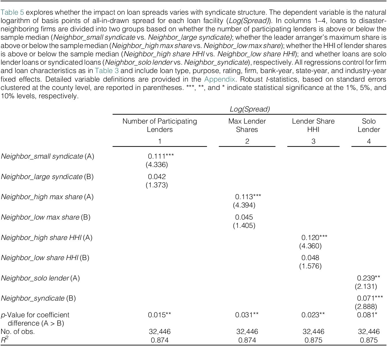
We next explore whether loan syndications affect bankers’ reactions to salient disaster events. We find that the positive impact on loan spreads is significantly stronger when the syndicate is more concentrated, that is, when there are fewer lenders, when the leader arranger retains a larger share, and when the Herfindahl–Hirschman Index (HHI) of lender shares is higher. Since concentrated syndicates weaken group decision-making by centralizing power with lead arrangers, who may be more sensitive to perceived disaster risks due to reduced risk sharing, these results suggest that group decision-making might attenuate behavior biases.
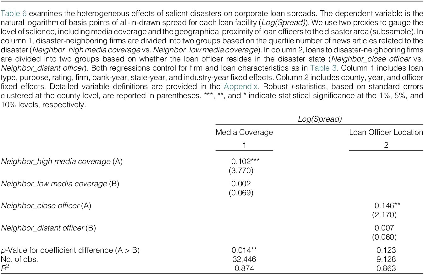
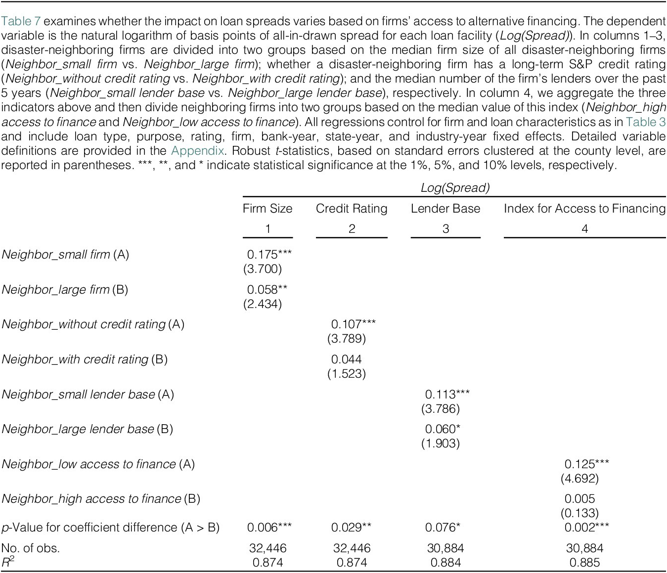
We also exploit two valuable features to strengthen the salience interpretation. First, we consider the influence of news coverage and find that the documented effect is stronger for natural disasters with higher news coverage. Second, we utilize the location information of loan officers in a subsample where we could identify their residential locations, and document a stronger effect for loan officers residing in the disaster-affected state. As another cross-sectional analysis, we assess the impact of borrowers’ potential bargaining power with the bank and find that smaller firms, firms with a smaller lender base, and firms without access to the public debt market are more vulnerable to banks’ overreaction.
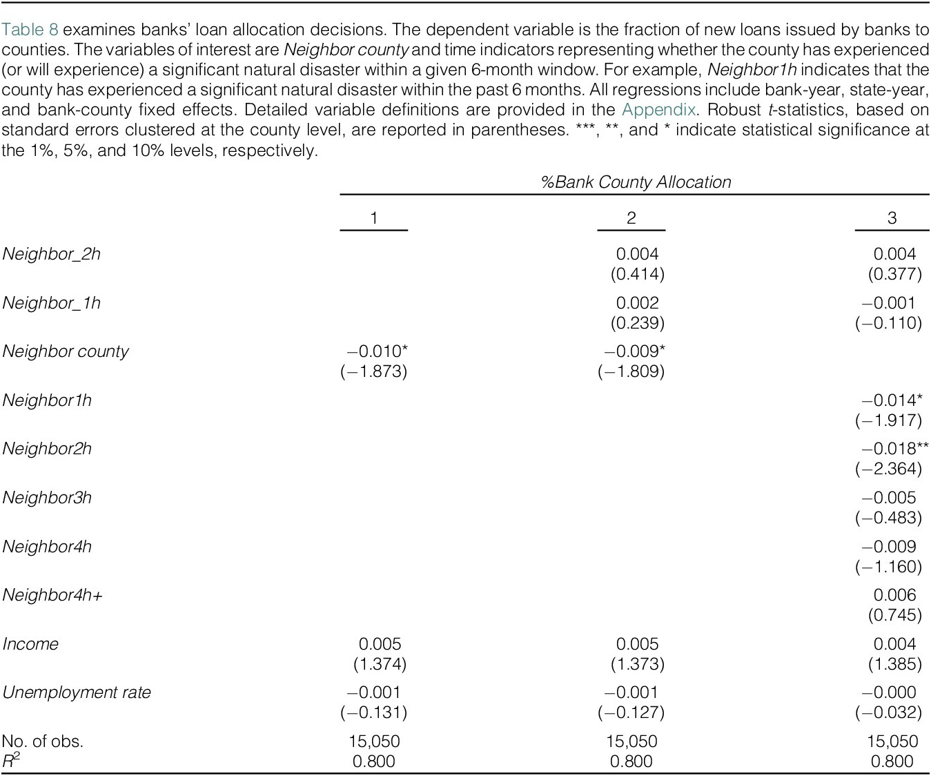
After documenting the impact on the intensive margin, we next explore banks’ reaction at the extensive margin. In particular, we examine whether banks temporarily adjust their portfolios away from firms located in the neighborhood area due to overreaction to natural disasters. Consistent with our salience hypothesis, we find that banks allocate a smaller amount of new loans to firms in neighboring counties following a salient natural disaster. These results are consistent with Alok, Kuma, and Wermers (Reference Alok, Kuma and Wermers2020), who document similar patterns of behavior among mutual fund managers operating within regions affected by major disasters.
We also investigate the real impact of banks’ salience bias on affected firms by examining firms’ investment-to-cash flow sensitivity. We find that investment-to-cash flow sensitivity increases for firms with major operations in the neighboring counties of the disaster area, especially for those without access to the public bond market. Our results indicate that the increased financing costs due to banks’ salience bias lead to heightened financial constraints for disaster-neighboring firms, particularly those with limited access to capital. Performing the analysis at the county level yields a similar conclusion.
We evaluate a number of alternative interpretations for our findings. First, we find no evidence of fundamental deterioration among neighboring firms, and the results persist after excluding firms most exposed to potential spillover effects. Second, we find no postdisaster changes in bank deposits, and the findings remain robust after excluding banks heavily exposed to affected regions. Third, the results remain unchanged after accounting for managers’ expressed disaster and climate risk concerns, suggesting that rent extraction is unlikely to explain our findings.
We also conduct a battery of tests to confirm the robustness of our results. Our findings remain robust to alternative definitions of neighboring firms, the exclusion of hurricane events and coastal areas, and the exclusion of the banking crisis period. We also show that our results are not sensitive to the way we construct the sample or alternative model specifications. Taken together, our study suggests that bank lenders are subject to salience bias when assessing their clients’ disaster risk, leading to capital constraints for affected firms.
Our article contributes to the literature in a number of dimensions. First, it adds to the growing literature documenting natural disaster-induced salience bias among economic agents. In particular, we complement Dessaint and Matray (Reference Dessaint and Matray2017) and Alok, Kuma, and Wermers (Reference Alok, Kuma and Wermers2020) by focusing on bank lenders, sophisticated financial intermediaries who presumably are more concerned about downside risks and whose actions play a central role in credit allocation. We show that bank lenders overweight recent and vivid disaster information when forming beliefs about borrowers’ disaster risk, leading them to charge significantly higher loan spreads to firms located near disaster areas following severe events. By documenting salience-driven overreaction in bank lending, our study contributes to ongoing debates on the prevalence and boundaries of behavioral biases in financial markets.
Second, our article contributes to the literature on collective versus individual decision-making. Research in behavioral economics and psychology indicates that groups often behave systematically differently from individuals, with group decision-making outperforming individuals in some cases, while individuals achieve better outcomes in others (e.g., Kerr, MacCoun, and Kramer (Reference Kerr, MacCoun and Kramer1996), Charness and Sutter (Reference Charness and Sutter2012)). Loan syndicates operate through a collective decision-making process, and our findings indicate that salience bias persists in this context. Notably, however, we find that the bias diminishes when the syndicate is less concentrated, suggesting that group decision-making may help attenuate behavioral biases. Our results therefore highlight the potential for institutional mechanisms to help mitigate such biases.
Third, we add to an important literature regarding bankers’ behavioral biases (see a survey by Malmendier (Reference Malmendier, Bernheim, DellaVigna and Laibson2018)). A few recent papers have documented behavioral biases in lending decisions, with a focus on how behavioral biases hinder lenders’ ability to effectively incorporate soft information and/or process accounting information. For example, Cortés, Duchin, and Sosyura (Reference Cortés, Duchin and Sosyura2016) provide microlevel evidence on the role of sentiment in loan officers’ credit approval decisions using daily variation in local sunshine as an instrument for sentiment. Campbell, Loumioti, and Wittenberg-Moerman (Reference Campbell, Loumioti and Wittenberg-Moerman2019) show that the cognitive constraints of loan officers can negatively affect the quality of loans they grant. Focusing on small business lending, Liu (Reference Liu2022) finds that lenders rely on salient hard information to guide their acquisition of soft information. Huo, Sun, Tai, and Xuan (Reference Huo, Sun, Tai and Xuan2024) show that exposure to foreclosure news can influence loan officers’ lending decisions in the United States mortgage market. Relatedly, our article also adds to the literature on how personal experiences affect lenders’ decisions (Malmendier (Reference Malmendier2021)). Koudijs and Voth (Reference Koudijs and Voth2016) show that lenders’ bankruptcy experience may have adverse effects on their subsequent risk-taking behavior. Carvalho, Gao, and Ma (Reference Carvalho, Gao and Ma2023) find that the experience of a housing market boom could bias loan officers’ assessment of the risk of their borrowers. We complement these studies by examining natural disaster-related experiences.
Finally, our article is related to the growing literature on investors’ consideration of climate risk (e.g., Bolton and Kacperczyk (Reference Bolton and Kacperczyk2021)) and particularly those works that study how lenders’ respond to climate-related risk. Studies find that lenders incorporate environmental and climate change concerns (Chava (Reference Chava2014), Nguyen, Ongena, Qi, and Sila (Reference Nguyen, Ongena, Qi and Sila2022)) and climate transition risk (e.g., Ivanov, Kruttli, and Watugala (Reference Ivanov, Kruttli and Watugala2024)) in their lending decisions. Focusing on natural disasters, Ouazad and Kahn (Reference Ouazad and Kahn2022) show that banks are more likely to approve mortgages that can be securitized in recently disaster-affected areas. Our study shows that banks also adjust their loan pricing for disaster-neighboring firms and such transitory adjustment is likely to be due to bankers’ salience bias.
The rest of the article is organized as follows: Section II describes our sample construction and empirical strategy. Sections III–V present our empirical results. Section VI concludes.
II. Data and Empirical Methodology
A. Data
To construct our sample, we start with all corporate syndicated loans issued to the U.S. firms that have financial information available from Compustat during the period 1987–2017. Data on corporate loans are collected from the DealScan database maintained by the Loan Pricing Corporation, which contains information about loan pricing and various loan terms at origination, such as loan size, use of collateral, and covenants. We match the loan data with Compustat firms using the most updated DealScan–Compustat link file, maintained by Michael Roberts and Wharton Research Data Services (Chava and Roberts (Reference Chava and Roberts2008)). Loans with information missing on key terms, such as loan spread, lender identity, or loan amount, are excluded from the sample. We also remove loans issued to financial firms (SIC 6000–6999) and regulated utilities (SIC 4900–4949).
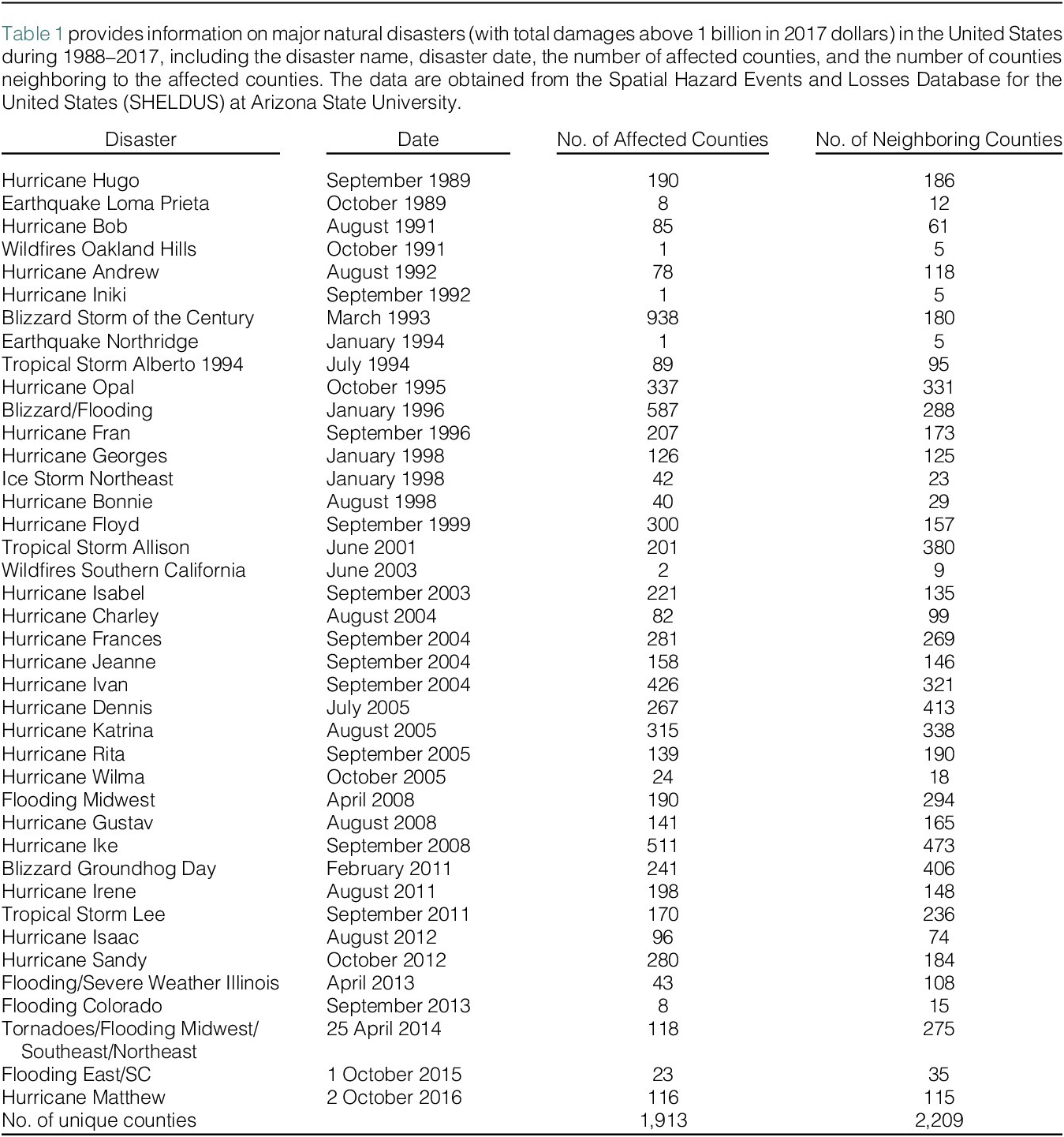
We obtain data on major natural disasters from the Spatial Hazard Events and Losses Database for the United States (SHELDUS) at Arizona State University. For each event, SHELDUS provides information on the event dates, disaster types, property damages, fatalities, and affected county locations of major natural disasters in the United States. To ensure that an event is salient enough, we focus on disasters with total estimated damages above $1 billion 2017 dollars and with a duration less than 30 days (Barrot and Sauvagnat (Reference Barrot and Sauvagnat2016)). This filtering procedure leaves us with 40 major disasters during 1987–2017. Table 1 reports basic information about these disasters, such as disaster name, disaster date, and the number of counties affected by each disaster and counties neighboring to them. The events are not clustered but rather dispersed over our sample period.

TABLE 1 Long description
The table contains four columns: Disaster, Date, Number of Affected Counties, and Number of Neighboring Counties.
Key entries include:
* Hurricane Hugo, September 1989: 190 affected, 186 neighboring.
* Earthquake Loma Prieta, October 1989: 8 affected, 12 neighboring.
* Hurricane Bob, August 1991: 85 affected, 61 neighboring.
* Wildfires Oakland Hills, October 1991: 1 affected, 5 neighboring.
* Hurricane Andrew, August 1992: 78 affected, 118 neighboring.
* Hurricane Iniki, September 1992: 1 affected, 5 neighboring.
* Blizzard Storm of the Century, March 1993: 938 affected, 180 neighboring.
* Earthquake Northridge, January 1994: 1 affected, 5 neighboring.
* Tropical Storm Alberto 1994, July 1994: 89 affected, 95 neighboring.
* Hurricane Opal, October 1995: 337 affected, 331 neighboring.
* Blizzard/Flooding, January 1996: 587 affected, 288 neighboring.
* Hurricane Fran, September 1996: 207 affected, 173 neighboring.
* Hurricane Georges, January 1998: 126 affected, 125 neighboring.
* Ice Storm Northeast, January 1998: 42 affected, 23 neighboring.
* Hurricane Bonnie, August 1998: 40 affected, 29 neighboring.
* Hurricane Floyd, September 1999: 300 affected, 157 neighboring.
* Tropical Storm Allison, June 2001: 201 affected, 380 neighboring.
* Wildfires Southern California, June 2003: 2 affected, 9 neighboring.
* Hurricane Isabel, September 2003: 221 affected, 135 neighboring.
* Hurricane Charley, August 2004: 82 affected, 99 neighboring.
* Hurricane Frances, September 2004: 281 affected, 269 neighboring.
* Hurricane Jeanne, September 2004: 158 affected, 146 neighboring.
* Hurricane Ivan, September 2004: 426 affected, 321 neighboring.
* Hurricane Dennis, July 2005: 267 affected, 413 neighboring.
* Hurricane Katrina, August 2005: 315 affected, 338 neighboring.
* Hurricane Rita, September 2005: 139 affected, 190 neighboring.
* Hurricane Wilma, October 2005: 24 affected, 18 neighboring.
* Flooding Midwest, April 2008: 190 affected, 294 neighboring.
* Hurricane Gustav, August 2008: 141 affected, 165 neighboring.
* Hurricane Ike, September 2008: 511 affected, 473 neighboring.
* Blizzard Groundhog Day, February 2011: 241 affected, 406 neighboring.
* Hurricane Irene, August 2011: 198 affected, 148 neighboring.
* Tropical Storm Lee, September 2011: 170 affected, 236 neighboring.
* Hurricane Isaac, August 2012: 96 affected, 74 neighboring.
* Hurricane Sandy, October 2012: 280 affected, 184 neighboring.
* Flooding/Severe Weather Illinois, April 2013: 43 affected, 108 neighboring.
* Flooding Colorado, September 2013: 8 affected, 15 neighboring.
* Tornadoes/Flooding Midwest/Southeast/Northeast, 25 April 2014: 118 affected, 275 neighboring.
* Flooding East/S C, 1 October 2015: 23 affected, 35 neighboring.
* Hurricane Matthew, 2 October 2016: 116 affected, 115 neighboring.
The final row indicates the number of unique counties: 1,913 affected and 2,209 neighboring.
We determine whether a borrowing firm is affected by a disaster event based on the actual location of its operation.Footnote 2 Specifically, we obtain firms’ geographical footprints from the National Establishment Time Series (NETS) database, which provides annual establishment-level data on U.S. businesses and establishments from 1989 onward. For years prior to 1989, we use 1989 values as proxies. We match firms in our sample to NETS based on the name and address of the firm’s headquarters. Information on historical headquarters locations is obtained from Bill McDonald’s 10-X Header Database, which records firms’ reported addresses at the time of each SEC filing.Footnote 3 For firms without electronic filings prior to 1994, we assign the headquarters location based on the earliest available filing.
B. Empirical Methodology
We rely on both the occurrence of disasters and the exposure of the borrower to the disaster area to identify situations where a bank’s perception of the borrowing firm’s natural disaster risk could increase significantly. While it is highly probable that lenders’ risk perception in a disaster-affected area will change after the event, loans to firms in these areas are initially excluded from our main analysis. This exclusion is necessary as these firms’ fundamentals are likely to be affected by the disaster; including them would make it difficult to isolate the impact of salience bias on the cost of borrowing. Barrot and Sauvagnat (Reference Barrot and Sauvagnat2016) show that the effects of natural disasters on affected firms can last for more than 1 year (i.e., five quarters). Therefore, a firm in a disaster area is considered a disaster-affected firm and any loan issued to such firms within 24 months of the disaster is excluded from our analysis.
Among the remaining loans, we identify disaster-neighboring firms based on the locations of corporate establishments obtained from the NETS database. To do so, for each disaster event, we identify the neighboring counties of each disaster-affected county. Specifically, we collect information on county adjacency from the National Bureau of Economic Research and match each affected county with its five closest nonaffected counties.Footnote 4 Firms that derive more than 50% of their sales from these neighboring counties are categorized as disaster-neighboring firms (referred to as neighboring firms for brevity), while the rest are labeled as remote firms.
By construction, disaster-neighboring and remote firms in our sample are unlikely to be significantly and directly affected by the natural disaster. However, from the perspective of bank lenders, the perceived risk of being struck is likely to be higher for firms in the neighborhood of the disaster area. Therefore, we assess the potential impact of salience bias by comparing bank loans granted to neighboring firms following the disaster with loans to other firms.
To examine whether bank lenders respond differently to neighboring firms following a disaster, we estimate the following OLS regressions:

The observation is at the loan–bank level, which means that in a loan facility with multiple lead lenders, we treat each lender as a separate observation.Footnote 5 This type of analysis allows us to capture heterogeneity across different bank lenders. In this specification, f denotes the loan facility, i denotes the borrowing firm, b denotes the bank, t denotes the loan initiation year, c (s) denotes the county (state) in which the borrowing firm’s headquarters is located, and j denotes the industry of the borrowing firm. The dependent variable is Log(Spread) f,i,b,t, the natural logarithm of the all-in-drawn spread (in basis points) for loan facility f of firm i issued by bank b in year t. The explanatory variable of interest is Neighbor, an indicator variable that equals 1 if the borrowing firm is a disaster-neighboring firm within 24 months of a natural disaster, and 0 otherwise. According to Rhodes, Campbell, and Dawson (Reference Rhodes, Campbell and Dawson2004) and Murfin (Reference Murfin2012), an average loan is negotiated 2–3 months in advance of the legal effective date of the loan. To account for this time lag, we lag the loan starting date in DealScan by 3 months.Footnote 6
We include a number of firm characteristics that might affect loan spreads, including firm size (natural logarithm of total assets), cash holding, market-to-book ratio, financial leverage, ROA, asset tangibility, and Z-score (e.g., Lin, Ma, Malatesta, and Xuan (Reference Lin, Ma, Malatesta and Xuan2011)). All these firm characteristics are measured at the fiscal year prior to the loan initiation. To control for unobservable time-invariant heterogeneity across firms, we further include firm fixed effects (δi) in the regression. In addition, we control for various loan characteristics, including loan size, loan maturity, prior lending relationship, loan types (i.e., term loans, revolvers longer than 1 year, revolvers shorter than 1 year, and 364-day loans), loan purposes (i.e., general corporate purpose, refinancing, acquisition, backup line for commercial paper, and others), and a dummy variable indicating whether the loan includes a contingent performance-based pricing clause.
In our primary specification, we include bank-year fixed effects (θb,t) to control for time-varying heterogeneity across banks. This is important because natural disasters may affect banks’ fundamentals in different ways, such as their exposure to local deposit markets or their ability to assess borrower risk following extreme events. Bank-year fixed effects absorb these bank-level characteristics and thus control for the impact of bank fundamentals on the supply of bank loans. This approach strengthens identification by comparing lending by the same bank to firms located inside versus outside neighboring disaster-affected areas within the same year, thereby accounting for unobserved, time-varying bank characteristics that could otherwise bias the estimates. In addition, state-year fixed effects (ϑs,t) are included, allowing us to compare loans issued to borrowers in the same state and year. Finally, we include industry-year fixed effects (μj,t) to address time-varying differences across industries.
C. Summary Statistics
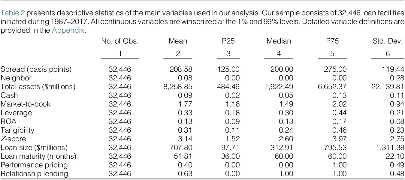
After requiring nonmissing values for our main control variables, we obtain a sample of 32,446 loans during the 1987–2017 period issued by 1,308 lenders to 4,349 unique public firms. Table 2 reports the summary statistics for various firm and loan characteristics. Detailed definitions of the variables are provided in the Appendix. All dollar values are adjusted to 2017 dollars using the Consumer Price Index data from the Bureau of Labor Statistics. To mitigate the influence of outliers, all continuous variables are winsorized at the 1st and 99th percentiles. The average loan spread in our sample is about 209 basis points, and 8% of loans are issued to borrowers whose main operations are in the neighborhood of a county hit by a natural disaster in the preceding 24 months. In our sample, an average borrowing firm has total assets of $ 8.3 billion, cash ratio of 0.09, market-to-book of 1.77, book leverage of 0.33, ROA of 0.13, PPE-to-assets ratio (Tangibility) of 0.31, and Z-score of 3.14. On average, loans have a size of around $708 million and a maturity of around 52 months. Among these loans, 40% use performance pricing and 63% are relationship lending.

TABLE 2 Long description
The table consists of 13 rows of variables and 6 columns of statistics. All variables have 32,446 observations.
* Spread (basis points): Mean 208.58, P 25 125.00, Median 200.00, P 75 275.00, Std. Dev. 119.44.
* Neighbor: Mean 0.08, P 25 0.00, Median 0.00, P 75 0.00, Std. Dev. 0.28.
* Total assets ($millions): Mean 8,258.85, P 25 484.46, Median 1,922.49, P 75 6,652.37, Std. Dev. 22,139.81.
* Cash: Mean 0.09, P 25 0.02, Median 0.05, P 75 0.13, Std. Dev. 0.11.
* Market-to-book: Mean 1.77, P 25 1.18, Median 1.49, P 75 2.02, Std. Dev. 0.94.
* Leverage: Mean 0.33, P 25 0.18, Median 0.30, P 75 0.44, Std. Dev. 0.21.
* R O A: Mean 0.13, P 25 0.09, Median 0.13, P 75 0.17, Std. Dev. 0.08.
* Tangibility: Mean 0.31, P 25 0.11, Median 0.24, P 75 0.46, Std. Dev. 0.23.
* Z-score: Mean 3.14, P 25 1.52, Median 2.60, P 75 3.97, Std. Dev. 2.75.
* Loan size ($millions): Mean 707.80, P 25 97.71, Median 312.91, P 75 795.53, Std. Dev. 1,311.38.
* Loan maturity (months): Mean 51.81, P 25 36.00, Median 60.00, P 75 60.00, Std. Dev. 22.10.
* Performance pricing: Mean 0.40, P 25 0.00, Median 0.00, P 75 1.00, Std. Dev. 0.49.
* Relationship lending: Mean 0.63, P 25 0.00, Median 1.00, P 75 1.00, Std. Dev. 0.48.
III. Empirical Results
A. Baseline Results
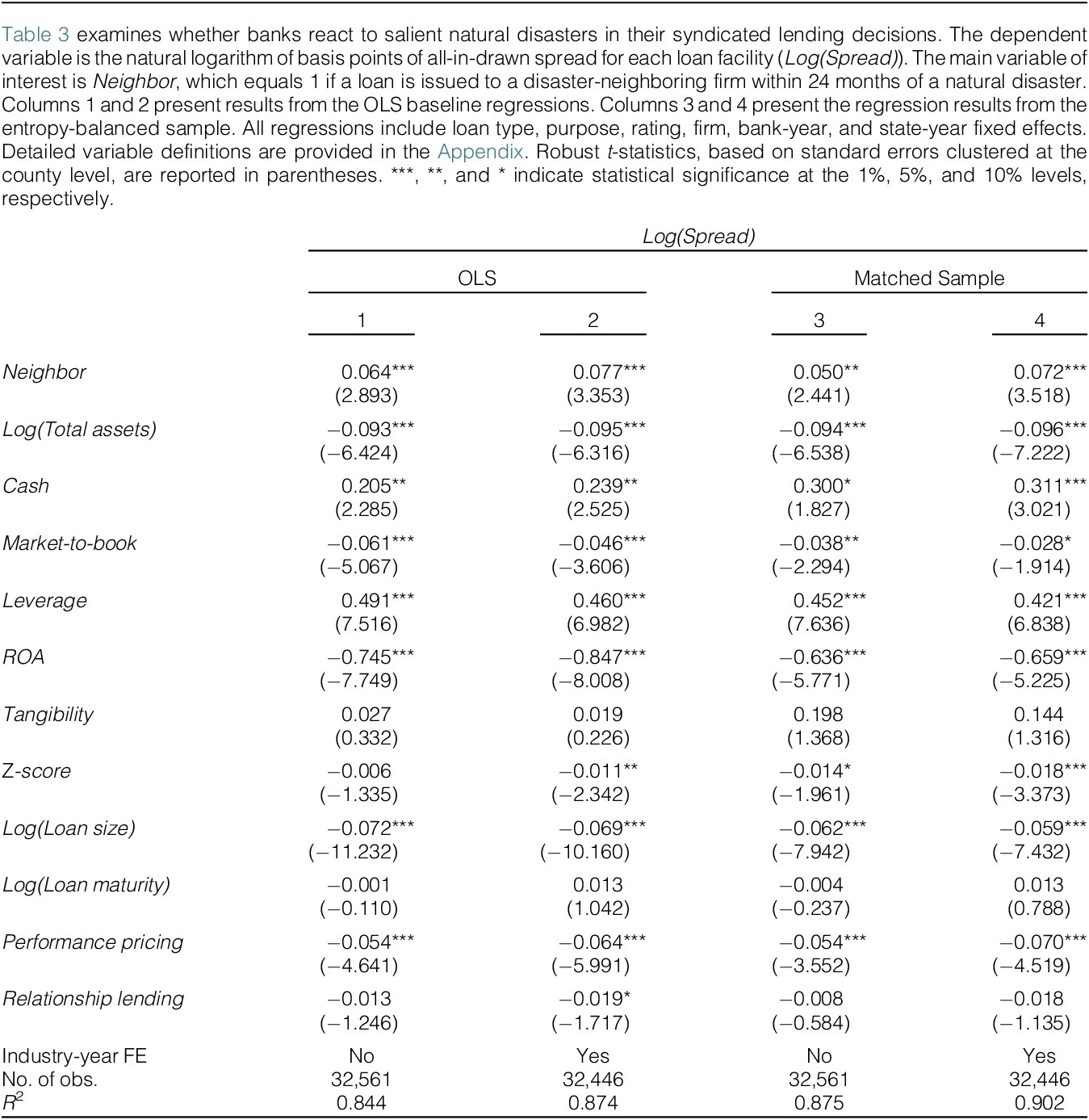
Table 3 presents our baseline results. All t-statistics reported in parentheses are based on standard errors clustered at the county level. In column 1, we include firm and loan controls, as well as firm, bank-year, and state-year fixed effects. In column 2, we further include industry-year fixed effects. We first find that the estimated coefficients of control variables are largely consistent with prior literature. For instance, larger firms and firms with higher market-to-book ratio, lower financial leverage, and higher profitability (ROA) are associated with lower bank loan costs. More importantly, we find that the coefficient of Neighbor is positive and statistically significant at the 1% level in both columns, suggesting that within 24 months of a natural disaster, banks charge higher loan spreads to firms operating in the neighboring area of the disaster than they charge to other firms.

TABLE 3 Long description
The table presents regression results for the dependent variable Log(Spread). The columns are numbered 1 through 4. Columns 1 and 2 use O L S, while columns 3 and 4 use a Matched Sample.
Key variable results:
* Neighbor: Coefficients are 0.064 (t = 2.893), 0.077 (t = 3.353), 0.050 (t = 2.441), and 0.072 (t = 3.518). All are statistically significant at the 1% or 5% level.
* Log(Total assets): Coefficients are approximately -0.094 across all models, all significant at the 1% level.
* Cash: Positive coefficients ranging from 0.205 to 0.311, significant in most models.
* Market-to-book: Negative coefficients ranging from -0.061 to -0.028.
* Leverage: Positive coefficients ranging from 0.421 to 0.491, all significant at the 1% level.
* R O A: Negative coefficients ranging from -0.636 to -0.847, all significant at the 1% level.
* Tangibility: Positive but statistically insignificant coefficients.
* Z-score: Negative coefficients ranging from -0.006 to -0.018.
* Log(Loan size): Negative coefficients ranging from -0.059 to -0.072, all significant at the 1% level.
* Log(Loan maturity): Statistically insignificant coefficients near zero.
* Performance pricing: Negative coefficients ranging from -0.054 to -0.070, all significant at the 1% level.
* Relationship lending: Negative coefficients ranging from -0.008 to -0.019.
Fixed Effects and Statistics:
* Industry-year F E: ‘No’ for columns 1 and 3; ‘Yes’ for columns 2 and 4.
* Number of observations: 32,561 for columns 1 and 3; 32,446 for columns 2 and 4.
* R-squared: Values are 0.844, 0.874, 0.875, and 0.902 for columns 1 through 4 respectively.
The effect on loan spreads is also economically meaningful. Estimates from column 1 indicate that if a firm mainly operates in the neighboring area of a region hit by a natural disaster in the prior 2 years, its loan spreads are 6.4% higher than those paid by other firms. Given the average loan spreads of 209 basis points (bps), this corresponds to a 13.4 basis-point higher interest rate paid by neighboring firms within 24 months of a disaster. The economic magnitude is comparable to that of market-to-book (a 1-standard-deviation reduction in market-to-book increases the cost of bank loans by 12 bps) and ROA (12.5 bps). In Supplementary Material Table A1, we include loans to firms directly affected by natural disasters and compare the impact on loan pricing for directly affected firms with the impact observed for neighboring firms. We find that both neighboring and directly affected firms experience significant increases in loan spreads following natural disasters, with magnitudes that are similar across the two groups. This comparison provides a benchmark for interpreting the economic magnitude of the pricing response observed for neighboring firms and suggests that overreaction to salient disaster events may impose meaningful financing costs on borrowing firms.
Our results are consistent with our salience hypothesis that bank lenders respond differently to neighboring firms after a disaster. To mitigate the concern that our results are driven by fundamental differences between neighboring firms after the disaster and remote firms, we repeat our baseline analysis using an entropy-balanced sample. This technique has certain advantages over the propensity-score-matching method (e.g., Chapman, Miller, and White (Reference Chapman, Miller and White2019)). It assigns weights to control observations so that the distributional properties of the treatment group and the postweighting control group are virtually identical.
Specifically, via a maximum-entropy reweighting scheme (Hainmueller and Xu (Reference Hainmueller and Xu2013)), we perform entropy balancing on the first three moments (i.e., mean, variance, and skewness) of all firm covariates to ensure that the distributions of all included control variables are similar for neighboring firms and other firms. Table 3 columns 3 and 4 present the results, which are similar to those in columns 1 and 2, suggesting that, after a natural disaster, bank lenders tend to charge higher interest rates on loans for firms operating in the neighborhood of a disaster region.
B. Dynamic Trend
To further assess causality, we examine the dynamic effects of salient natural disasters on neighboring firms’ borrowing costs. This analysis helps address concerns that the observed effect is a result of preexisting trends or spurious correlation. In addition, it allows us to evaluate whether the effect is transitory, as suggested by Dessaint and Matray (Reference Dessaint and Matray2017) and Alok, Kuma, and Wermers (Reference Alok, Kuma and Wermers2020).
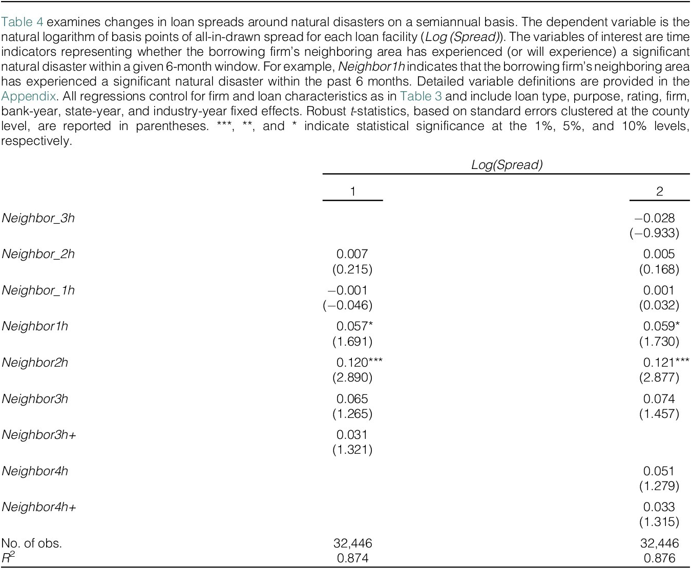
Specifically, we construct a series of time indicators, each capturing whether a borrowing firm’s neighboring area has experienced (or will experience) a significant natural disaster within a given 6-month window. We then replace Neighbor with these time indicators and re-estimate the baseline specification. For example, the indicator variable Neighbor1h equals 1 if the borrowing firm’s neighboring area experienced a significant natural disaster within the past 6 months. The coefficient estimates of the time indicators for the periods before and after the disaster are plotted in Figure 1 and reported in Table 4.
Figure 1 plots the coefficient estimates along with their 90% confidence intervals in the dynamic trend analysis showing changes in loan spreads around natural disasters on a semiannual basis. The time indicators on the x-axis represent whether the borrowing firm’s neighboring area has experienced a significant natural disaster within a given 6-month period. For example, “1” indicates that the borrowing firm’s neighboring area has experienced a significant natural disaster within the past 6 months.

FIGURE 1 Long description
A line graph titled Dynamic Effect. The vertical Y-axis is labeled Coefficients and ranges from minus 0.1 to 0.2 in increments of 0.1. The horizontal X-axis is labeled Per Six-Month Relative to Disaster Date with markers at minus 3, minus 2, minus 1, 1, 2, 3, 4, and 4 plus. A vertical red line is positioned between minus 1 and 1, representing the disaster event.
Data points are represented by blue dots with dashed vertical error bars indicating 90 percent confidence intervals.
* To the left of the red line (pre-disaster):
- At minus 3, the coefficient is slightly below 0.
- At minus 2 and minus 1, the coefficients are near 0, with confidence intervals crossing the zero line.
* To the right of the red line (post-disaster):
- At 1, the coefficient rises to approximately 0.06.
- At 2, the coefficient peaks at approximately 0.12.
- At 3, 4, and 4 plus, the coefficients gradually decline toward 0.04, though they remain positive.
The confidence intervals for all post-disaster periods except 3 and 4 are entirely above the zero line, indicating a statistically significant increase in loan spreads following the disaster.

TABLE 4 Long description
A regression table with two columns representing different model specifications for the dependent variable Log open parenthesis Spread close parenthesis. The rows list coefficients for time-indexed variables related to natural disasters in neighboring areas, with t-statistics in parentheses below each coefficient.
* Neighbor underscore 3 h: Column 2 shows minus 0.028 with a t-statistic of minus 0.933.
* Neighbor underscore 2 h: Column 1 is 0.007 (0.215); Column 2 is 0.005 (0.168).
* Neighbor underscore 1 h: Column 1 is minus 0.001 (minus 0.046); Column 2 is 0.001 (0.032).
* Neighbor 1 h: Column 1 is 0.057* (1.691); Column 2 is 0.059* (1.730).
* Neighbor 2 h: Column 1 is 0.120*** (2.890); Column 2 is 0.121*** (2.877).
* Neighbor 3 h: Column 1 is 0.065 (1.265); Column 2 is 0.074 (1.457).
* Neighbor 3 h plus: Column 1 is 0.031 (1.321).
* Neighbor 4 h: Column 2 is 0.051 (1.279).
* Neighbor 4 h plus: Column 2 is 0.033 (1.315).
Summary statistics at the bottom show:
* Number of observations: 32,446 for both columns.
* R super 2: 0.874 for Column 1 and 0.876 for Column 2.
Asterisks indicate statistical significance: *** for 1 percent, ** for 5 percent, and * for 10 percent levels.
Two key findings emerge. First, the coefficients for predisaster periods (i.e., −3 h to −1 h) are not statistically different from 0, indicating that the increase in loan spreads does not occur prior to the disaster. Second, the postdisaster increase in loan spreads diminishes within 1 year after the disaster. These patterns support a causal interpretation of our results and align with prior evidence that the effect of salience bias decreases over time (Dessaint and Matray (Reference Dessaint and Matray2017), Alok, Kuma, and Wermers (Reference Alok, Kuma and Wermers2020)). Overall, we find no significant change in loan spreads before a neighboring disaster, but a significant increase immediately afterward.
C. The Impact of the Syndicate Structure
The loans in our sample are mostly syndicated, reflecting a collective lending arrangement where multiple banks jointly negotiate and approve terms. We next explore whether this structured collaboration affects banks’ reactions to salient disaster events. We argue that broadly syndicated loans facilitate greater group collaboration, while concentrated syndicates weaken group decision-making by centralizing power with lead arrangers—who may be more sensitive to perceived disaster risks due to reduced risk sharing. If group decision-making attenuates behavior biases, we expect a stronger salience effect in loans with more concentrated syndicate structures.
To test this conjecture, we construct three measures of syndicate concentration: the number of lenders in the syndicate, the maximum share held by the leader arranger, and the HHI of lender shares. We then divide loans to neighboring firms into two groups based on whether the number of lenders is above (i.e., Neighbor_large syndicate = 1) or below the sample median; whether the leader arranger’s maximum share is above (i.e., Neighbor_high max share = 1) or below the sample median; and whether the HHI of lender shares is above (i.e., Neighbor_high share HHI = 1) or below the sample median.
Columns 1–3 of Table 5 report the results. We find that the positive impact on loan spreads is significantly stronger when the syndicate is more concentrated, that is, when there are fewer lenders, the leader arranger retains a larger share, or the HHI of lender shares is higher. In column 4, we examine extreme cases in DealScan where loans to neighboring firms have only one lender (a nonsyndicated loan). We find consistent results. The behavior biases are far more pronounced for solo-lender loans than for syndicated loans. Taken together, Table 5 demonstrates that a concentrated lender base amplifies salience bias, whereas a broad syndicate structure helps mitigate behavior biases.

TABLE 5 Long description
A statistical table with four columns representing different syndicate structure metrics. The dependent variable for all columns is Log(Spread).
* Column 1 (Number of Participating Lenders): Neighbor_small syndicate (A) has a coefficient of 0.111 (t-stat 4.336, significant at 1 percent). Neighbor_large syndicate (B) has a coefficient of 0.042 (t-stat 1.373). The p-value for the coefficient difference (A > B) is 0.015 (significant at 5 percent).
* Column 2 (Max Lender Shares): Neighbor_high max share (A) has a coefficient of 0.113 (t-stat 4.394, significant at 1 percent). Neighbor_low max share (B) has a coefficient of 0.045 (t-stat 1.405). The p-value for the coefficient difference (A > B) is 0.031 (significant at 5 percent).
* Column 3 (Lender Share H H I): Neighbor_high share H H I (A) has a coefficient of 0.120 (t-stat 4.360, significant at 1 percent). Neighbor_low share H H I (B) has a coefficient of 0.048 (t-stat 1.576). The p-value for the coefficient difference (A > B) is 0.023 (significant at 5 percent).
* Column 4 (Solo Lender): Neighbor_solo lender (A) has a coefficient of 0.239 (t-stat 2.131, significant at 5 percent). Neighbor_syndicate (B) has a coefficient of 0.071 (t-stat 2.888, significant at 1 percent). The p-value for the coefficient difference (A > B) is 0.081 (significant at 10 percent).
All columns report 32,446 observations with R-squared values ranging from 0.874 to 0.875.
D. Heterogeneous Effects
We next conduct several heterogeneity tests to better understand the mechanism of the impact. If it is salience bias that drives our results, we expect that the impact should be greater when the disaster events are more salient to bank officers. We use two proxies to measure the level of salience. The first one is media coverage. Greater media coverage of natural disasters likely increases the salience of the events. To test this conjecture, for each event listed in Table 1, we search for the disaster’s name in Factiva to obtain the total number of news articles related to the event within 3 months of the disaster’s occurrence. We then divide disaster-neighboring firms into two groups based on the number of news articles related to the disaster. Column 1 of Table 6 reports the results. Consistent with our conjecture, we find that the documented effect is driven by disasters with high media coverage (i.e., Neighbor_high media coverage = 1). The coefficient for the high-media-coverage subsample is positive and significant at the 1% level, and it is significantly greater than the coefficient for the low-media-coverage subsample, which is not statistically different from 0.

TABLE 6 Long description
A regression table with two columns. The dependent variable for both is Log(Spread).
Column 1: Media Coverage.
- Neighbor_high media coverage (A): coefficient 0.102 with a t-statistic of 3.770, significant at the 1 percent level.
- Neighbor_low media coverage (B): coefficient 0.002 with a t-statistic of 0.069.
- p-Value for coefficient difference (A > B): 0.014, significant at the 5 percent level.
- Number of observations: 32,446.
- R-squared: 0.874.
Column 2: Loan Officer Location.
- Neighbor_close officer (A): coefficient 0.146 with a t-statistic of 2.170, significant at the 5 percent level.
- Neighbor_distant officer (B): coefficient 0.007 with a t-statistic of 0.060.
- p-Value for coefficient difference (A > B): 0.123.
- Number of observations: 9,128.
- R-squared: 0.863.
The second measure is the geographical proximity of loan officers to the disaster area. The salience of a natural disaster should be greater when loan officers are located closer to the disaster region. While certain details about loan officers (such as names, titles, employers, etc.) can be manually collected from credit agreement documents that are filed to the Security Exchange Commission (SEC), obtaining precise information about the officer’s exact location is challenging. Nevertheless, we use the residential location of loan officers in their voting registration record to estimate their proximity to the disaster (Dagostino, Gao, and Ma (Reference Dagostino, Gao and Ma2023)).Footnote 7 We then define two indicator variables: Neighbor_close officer, which equals 1 if the loan officer resides in the disaster state, and Neighbor_distant officer, which equals 1 if the loan officer does not reside in the disaster state. Column 2 of Table 6 reports the results. The sample size is significantly reduced due to the availability of information on loan officers’ voting registration record. We find a large and statistically significant coefficient for the variable Neighbor_close officer, but a small and statistically insignificant coefficient for Neighbor_distant officer. While the coefficient difference between these coefficients is not statistically significant at the 10% level (p = 0.123), the pattern of results is consistent with the salience hypothesis.Footnote 8
In Table 7, we examine the role of firms’ access to external financing. If bankers’ salience bias leads to higher borrowing costs for firms, this effect should be most pronounced among bank-dependent borrowers with limited access to alternative financing options, and consequently, weaker bargaining power. Larger firms and firms with credit ratings arguably have better access to the capital markets. Moreover, firms with a larger lender base might be able to counteract the bias of a particular bank by potentially switching to alternative banks. Therefore, we define three indicator variables to proxy for a firm’s access to alternative financing: whether the firm’s market capitalization is above the median for all neighboring firms (column 1), whether it has a credit rating (column 2), and whether its number of lenders over the past 5 years is above the median for all neighboring firms (column 3). The results indicate that increased borrowing costs among neighboring firms are indeed concentrated on smaller firms, firms lacking credit ratings, and firms with a smaller lender base. In addition, we construct an index of access to external finance for each disaster-neighboring firm by aggregating the three indicators discussed previously. We then divide neighboring firms into two groups based on the median value of this index (column 4). As shown in column 4, the impact on loan spreads is positive and statistically significant at the 1% level for firms with low access to external finance (i.e., Neighbor_low access to finance = 1), and the effect is significantly greater than for firms with high access. Overall, the findings from these heterogeneous effect analyses provide clear evidence of salience bias affecting banks’ assessment of their borrowers’ natural disaster risk.

TABLE 7 Long description
A table with four columns representing different regression models for Log(Spread).
Column 1 (Firm Size):
- Neighbor_small firm (A): 0.175 (t-stat 3.700, significant at 1% level).
- Neighbor_large firm (B): 0.058 (t-stat 2.434, significant at 5% level).
- p-Value for coefficient difference (A > B): 0.006.
- Observations: 32,446. R-squared: 0.874.
Column 2 (Credit Rating):
- Neighbor_without credit rating (A): 0.107 (t-stat 3.789, significant at 1% level).
- Neighbor_with credit rating (B): 0.044 (t-stat 1.523).
- p-Value for coefficient difference (A > B): 0.029.
- Observations: 32,446. R-squared: 0.874.
Column 3 (Lender Base):
- Neighbor_small lender base (A): 0.113 (t-stat 3.786, significant at 1% level).
- Neighbor_large lender base (B): 0.060 (t-stat 1.903, significant at 10% level).
- p-Value for coefficient difference (A > B): 0.076.
- Observations: 30,884. R-squared: 0.884.
Column 4 (Index for Access to financing):
- Neighbor_low access to finance (A): 0.125 (t-stat 4.692, significant at 1% level).
- Neighbor_high access to finance (B): 0.005 (t-stat 0.133).
- p-Value for coefficient difference (A > B): 0.002.
- Observations: 30,884. R-squared: 0.885.
E. Robustness Tests
In this section, we conduct a set of tests to evaluate the robustness of our finding. The results are reported in the Supplementary Material Table A2. First, we use alternative definitions of Neighbor. In our main analysis, we define neighboring firms as those with more than 50% of sales generated from the disaster neighborhood area. Using two continuous measures of exposure—the share of sales and the share of employees in the disaster neighborhood area—we find consistent results, confirming that our results are not sensitive to the 50% sales cutoff.
Second, we remove hurricanes and the financial crisis period from our sample. As shown in Table 1, most of the natural disasters in our sample are hurricanes that predominantly affect coastal counties. We therefore repeat our baseline analysis by removing loans issued to hurricane-neighboring firms within 24 months of a hurricane. Our results remain robust. Furthermore, to mitigate the potential confounding effect of the financial crisis, we conduct an additional analysis excluding loans issued during 2007–2009. The results are similar.
Third, we conduct a package-level analysis. Multiple loan facilities can belong to the same loan package and be governed by the same contract (e.g., Bushman, Gao, Martin, and Pacelli (Reference Bushman, Gao, Martin and Pacelli2021)). We therefore repeat our baseline analysis using package–bank-level observations, where the dependent variable is the weighted average loan spread, with facility amounts used as weights. The results remain robust.
Four, we control for seasonality in the analysis. Natural disasters (e.g., hurricanes), corporate business operations, and credit markets can have seasonality (Murfin and Petersen (Reference Murfin and Petersen2016)). To account for the potential impact of seasonal factors, we include quarter fixed effects in the regressions and find similar results.
Fifth, we include firm–bank fixed effects. Unobserved stable factors, such as long-term lending relationships, could influence loan pricing. As a further robustness check, we estimate a specification with firm–bank pair fixed effects, effectively restricting identification to loan pricing changes within the same firm–bank pair over time. Our results remain robust.Footnote 9
Sixth, we address the issues of repeated observations by adjusting the weights. Because the number of repeated firm-facility observations increases with the number of participating banks, facilities involving more banks receive greater weight in the estimation. To address this issue, we follow prior literature (Armstrong, Jagolinzer, and Larcker (Reference Armstrong, Jagolinzer and Larcker2010), Stuart (Reference Stuart2010)) and reweight repeated observations. Specifically, we conduct a weighted least squares (WLS) analysis, assigning each observation a weight inversely proportional to its sample frequency. The results remain robust.
Finally, we ensure that our results are robust to alternative estimation methods. We adopt two additional approaches. First, we implement a DID design using our pooled loan data (e.g., Wooldridge (Reference Wooldridge2019)). Specifically, we consider the first time a borrowing firm’s neighborhood experiences a disaster within our sample period as an exogenous shock and retain loans issued to the firm 2 years before and after the disaster. For each loan issued to a treated firm, we select five loans issued to firms that: i) were never neighbors to the disaster area; ii) belonged to the same industry and year as the treated firm; and iii) had the nearest score using the propensity score matching method based on all firm covariates. We then conduct a pooled DID regression using this much smaller sample. The results reported in Supplementary Material Table A3 indicate that loan spreads are higher for borrowers in the neighborhood of a disaster area within 2 years following the disaster.
Second, we construct a firm-year panel data and use a firm’s average cost of debt as a proxy for its bank loan costs. To be included in the sample, we retain only firms that have had bank loans during our sample period. Following the literature on the cost of debt, we measure a firm’s cost of debt in year t as the ratio of its interest expenses in year t and the average total debt in years t – 1 and t. We then conduct a series of DID estimations using these panel data, with cost of debt as the dependent variable. Supplementary Material Figure A1 presents the dynamic effect of natural disasters on neighboring firms’ cost of debt using the two-way fixed effects (TWFE) estimator and four alternative dynamic DID estimators developed by de Chaisemartin and D’Haultfoeuille (Reference De Chaisemartin and D’Haultfoeuille2020), Callaway and Sant’Anna (Reference Callaway and Sant’Anna2021), Sun and Abraham (Reference Sun and Abraham2021), and Borusyak, Jaravel, and Spiess (Reference Borusyak, Jaravel and Spiess2024)). Similarly, there is no significant difference in the cost of debt prior to the occurrence of a natural disaster. The treatment effect mainly concentrates during and within the first year following the disaster year. However, we are cautious about drawing strong inferences due to the limitations of this coarse measure of bank loan costs in these analyses.
Overall, the findings from these analyses lend further support to our main argument that disasters in neighboring areas affect firms’ cost of debt in the subsequent year and mitigate the concern that this effect is driven by omitted variables.
IV. Alternative Explanations and Additional Analyses
A. Alternative Explanations
In this section, we evaluate potential alternative explanations that may confound our interpretation. Specifically, we discuss the following possible interpretations: regional spillovers, limited credit supply, and lender rent extraction.
1. Regional Spillovers
It is plausible that neighboring firms in our sample are adversely affected by the natural disasters due to regional spillover, which in turn affects their cost of borrowing. We take several approaches to explore whether this alternative explanation drives our findings. First, we examine firm fundamentals that directly affect the cost of borrowing, and check whether disaster-neighboring borrowers are fundamentally weaker than remote borrowers. Supplementary Material Table A4, Panel A, shows that neighboring borrowers in our sample are not fundamentally different from remote borrowers after their neighborhood experienced a disaster.
Regional spillovers may also lead to a deterioration in local economic conditions that in turn cause higher borrowing cost for neighboring firms. While there is no evidence that nearby counties are adversely affected (e.g., Tran and Wilson (Reference Tran and Wilson2024)), we address this possibility by augmenting the baseline model with time-varying local economic conditions as additional controls. In addition, because the negative impact of natural disasters may propagate through production network, we exclude loans to firms with major customers or suppliers in the disaster zone, identified using the Compustat Segment database. Finally, to further ensure that our findings are not driven by regional spillover, we use stock price comovements to capture unobserved economic links between neighboring firms and disaster-affected firms and exclude loans issued to borrowers with high comovements with disaster-affected firms. Our findings continue to hold (Supplementary Material Table A4, Panel B).
To further verify the stability of credit default risk for neighboring firms, we conduct an event study to analyze implied volatility and CDS spreads around disaster events. Using each disaster’s start date as the event date, we calculate the average implied volatility in the days preceding and after the event and rating-adjusted cumulative abnormal CDS spread changes around the event. The results in Supplementary Material Table A5 suggest no significant changes in either implied volatility or CDS spreads for neighboring firms surrounding disastrous events. Collectively, these results suggest that the increase in loan spreads for neighboring firms is not a result of changes in firm fundamentals or regional spillovers.
2. Limited Credit Supply
Another possible explanation for our findings is that natural disasters may affect the lending capacity of banks located closer to disaster areas. That is, natural disasters may affect banks’ fundamentals and reduce their ability to lend, leading to an increase in the borrowing cost of neighboring firms. This concern is mitigated by the fact that we control for time-varying heterogeneity across banks using bank-year fixed effects, which help absorb the impact of bank-level credit supply. However, it is still plausible that the lending capacity is different for the same bank in different regions. To address this concern, we investigate whether banks experience any significant changes in their deposits in disaster-neighboring counties after a major disaster.
The results in Supplementary Material Table A6 show no significant changes in banks’ total deposits in disaster-neighboring counties following a major disaster. This finding aligns with Blickle, Hamerling, and Morgan (Reference Blickle, Hamerling and Morgan2025), who show that weather disasters have negligible or small effects on U.S. banks’ performance. In addition, to ensure that our results are not driven by bank fundamentals, in unreported analysis, we exclude loans issued by banks that lend significantly to regions directly impacted by natural disasters (i.e., banks with more than 1% of their loans allocated to firms in disaster areas), and our results remain consistent.
3. Rent Extraction
The final nonbehavioral interpretation of our findings we consider is rent extraction. Because corporate managers in neighboring firms may overestimate their disaster risk, banks could take advantage of this response by charging higher loan spreads, even though they understand that these borrowers’ objective disaster-related risk remains unchanged.
To evaluate this alternative explanation, we examine whether our results hold after we control for corporate managers’ potential overreaction to natural disasters, which unfortunately is difficult to measure. We measure managerial responses in two ways: i) following Dessaint and Matray (Reference Dessaint and Matray2017), we conduct textual analysis of SEC filings to count disaster-related mentions as a proxy for concern, and ii) we use the firm-level climate change risk measure from Sautner, Van Lent, Vilkov, and Zhang (Reference Sautner, Van Lent, Vilkov and Zhang2023)), based on earnings call transcripts that reference climate risk or uncertainty.
Supplementary Material Table A7 shows that our results remain consistent after we control for firm managers’ expressed concern about disaster risk. However, we acknowledge that both measures are noisy proxies that likely suffer from measurement error. Accordingly, these results should be interpreted with caution, as fully disentangling managerial versus lender overreaction is inherently challenging.
B. Impact on Loan Allocation Decisions
Our analysis thus far shows that, conditioning on lending activity, banks charge higher spreads on neighboring firms in the period following natural disasters, and that these effects are unlikely to be driven by firm, bank, or local economic fundamentals. Building on these findings, we next explore banks’ responses at the extensive margin. Specifically, we examine whether banks temporarily adjust their lending portfolios by reducing exposure to firms located in neighboring areas following salient natural disasters.
To answer this question, we conduct a bank-county-level analysis in which the dependent variable is the amount of new lending by a bank to firms in a given county (as recorded in DealScan), scaled by the bank’s total new loan issuance in that year. The results are reported in Table 8. All regressions include state-year, bank-year, and bank-county fixed effects, allowing us to compare changes in the fraction of lending by the same bank to the same county over time while controlling for time-varying factors at the state and bank levels.

TABLE 8 Long description
A statistical table with three columns labeled 1, 2, and 3, representing different regression models for the dependent variable percent Bank County Allocation.
Key variables and results include:
* Neighbor underscore 2 h: Model 2 is 0.004 (0.414); Model 3 is 0.004 (0.377).
* Neighbor underscore 1 h: Model 2 is 0.002 (0.239); Model 3 is minus 0.001 (minus 0.110).
* Neighbor county: Model 1 is minus 0.010* (minus 1.873); Model 2 is minus 0.009* (minus 1.809).
* Neighbor 1 h: Model 3 is minus 0.014* (minus 1.917).
* Neighbor 2 h: Model 3 is minus 0.018** (minus 2.364).
* Neighbor 3 h: Model 3 is minus 0.005 (minus 0.483).
* Neighbor 4 h: Model 3 is minus 0.009 (minus 1.160).
* Neighbor 4 h plus: Model 3 is 0.006 (0.745).
* Income: Model 1 is 0.005 (1.374); Model 2 is 0.005 (1.373); Model 3 is 0.004 (1.385).
* Unemployment rate: Model 1 is minus 0.001 (minus 0.131); Model 2 is minus 0.001 (minus 0.127); Model 3 is minus 0.000 (minus 0.032).
Summary statistics at the bottom show the Number of observations is 15,050 and the R-squared is 0.800 for all three models. Asterisks indicate statistical significance levels.
In column 1, we find a negative and statistically significant coefficient on Neighbor county, indicating that banks allocate a smaller amount of new lending to firms in neighboring counties following a natural disaster. In columns 2 and 3, we include time indicators that capture whether the county has experienced (or will experience) a significant natural disaster within a given 6-month window. The results show that the negative impact on lending does not occur prior to the disaster and is concentrated in the 12 months afterward. Overall, these results suggest a temporary reallocation of bank lending following natural disasters, providing corroborating evidence of a similar reaction at the extensive margin that is consistent with salience-driven overreaction in the aftermath of such events. These findings are analogous to the portfolio reallocation effects documented by Alok, Kuma, and Wermers (Reference Alok, Kuma and Wermers2020) for mutual fund managers’ equity holdings in regions affected by major disasters.
C. Additional Analysis
1. Evidence from Earthquakes Outside the United States
To further rule out alternative explanations, we perform tests using earthquakes outside the United States. In particular, we identify firms located in regions where earthquakes are frequently felt and then examine whether bank lenders charge higher loan spreads to these firms around the occurrence of extremely salient earthquakes outside the United States. Since these earthquakes are far away from the U.S., regional spillovers or bank credit supply channels should be absent. Finding an increase in loan spreads would provide further credence to our behavioral argument.
We collect information on earthquake intensity from the “Did you feel it?” surveys. We compute the average earthquake intensity felt over the period 1990–2016 for each zip code and then merge the zip-level earthquake intensity with firms in our sample using their headquarters locations. Firms with intensity level above the median are considered more “vulnerable” to earthquakes, as they are situated in seismic hazard zones. Next, we obtain information on the most significant earthquakes occurring outside the United States from the Significant Earthquake Database.
Supplementary Material Table A8 presents the results. We find that, after a sudden and salient earthquake outside the United States, banks charge higher interest rates to firms located in areas with higher earthquake intensity over the subsequent 12 months. Collectively, these results provide additional evidence that our findings from the main setting are unlikely to be driven by alternative explanations.
2. Impact on Nonprice Terms
We also examine whether, in addition to loan spreads, banks alter nonprice terms for loans issued to neighboring firms. Supplementary Material Table A9 reports the results. We do not find evidence that banks adjust performance-contingent pricing provision, loan size, or loan maturity for neighboring firms, suggesting that bank lenders do not adjust some nonprice terms for neighboring firms after a salient natural disaster.
V. The Real Impact on Financial Constraints
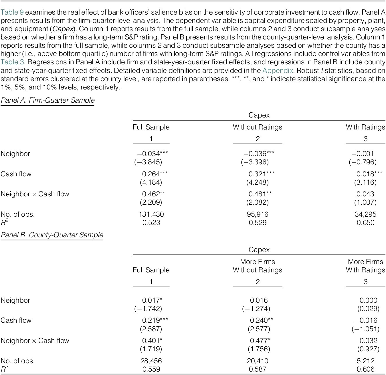
In this section, we examine the real effects of bank lenders’ salience bias on borrowing firms. Stiglitz and Weiss (Reference Stiglitz and Weiss1981) argue that lenders respond to higher risks by charging higher interest rates, employing nonprice risk-mitigating loan terms, and rationing capital. Thus, we expect that neighboring firms would suffer from greater capital constraints after a disaster event. To test this conjecture, we use the sensitivity of investments to cash flows (Fazzari, Hubbard, and Petersen (Reference Fazzari, Hubbard and Petersen1988)) as a proxy for financial constraints. According to Fazzari, Hubbard, and Petersen (Reference Fazzari, Hubbard and Petersen1988), financially constrained firms have a greater sensitivity of investment to cash flow than unconstrained firms. In our setting, after a disaster, neighboring firms would face higher costs of bank loans and, consequently, would need to rely more on internal cash flows to fund their investments. This would lead to greater investment-to-cash-flow sensitivity for these firms postdisaster, especially for those with limited access to external financing. To provide finer evidence, we use Compustat Quarterly data to form a firm-quarter sample, and estimate the following model specification:

Capex is a firm’s capital expenditure scaled by property, plant, and equipment. Neighbor equals 1 for disaster-neighboring firms within 24 months following a natural disaster. The main variable of interest is the interaction term Neighbor × Cash Flow, where Cash Flow is defined as the operating cash flow scaled by total assets. We control for various firm-level characteristics, including Log(Total assets), Market-to-book, Leverage, and Cash. Firm and state-year-quarter fixed effects are also included in the regressions. Because disaster-neighboring firms face higher borrowing cost postdisaster, we expect greater investment-to cash-flow sensitivity for these firms, that is, a positive and significant coefficient β.
Column 1 of Panel A in Table 9 reports the regression results. Consistent with prior literature, we observe a positive association between investment and cash flow. More importantly, the coefficient on Neighbor × Cash Flow is positive and statistically significant, indicating that disaster-neighboring firms experience an increase in the sensitivity of investment to cash flow postdisaster.

TABLE 9 Long description
Fallback
Our earlier results in Table 7 show that the increase in loan spreads is concentrated among neighboring firms with limited access to external financing. Therefore, disaster-neighboring firms with access to the bond market might be able to mitigate the increase in financial constraints. To examine this conjecture, we divide our sample into two groups: borrowers with long-term S&P credit ratings (comprising approximately one fourth of our sample) and borrowers without credit ratings, as the presence of a credit rating is a key proxy for access to public debt markets. Then, we run the regressions separately in these subsamples. We report the results in columns 2 and 3 of Table 9 Panel A. The regression results are consistent with our conjecture.
In Table 9, Panel B, we repeat the previous analysis using a county-quarter sample, where we average all variables across all firms in a county in each quarter using total assets as weights. This analysis allows us to assess the broader impact of bank lenders’ salience bias. In column 1, we present results from the full sample, while in columns 2 and 3, we conduct subsample analyses based on whether the county has a higher (i.e., above bottom quartile) number of firms with long-term S&P ratings. After controlling for county and state-year-quarter fixed effects, we find results that are consistent with those from our firm-level analysis. Overall, our findings indicate that bank lenders’ salience bias increases financial constraints for disaster-neighboring firms, particularly for firms without credit ratings.
VI. Conclusion
We provide empirical evidence showing that bank lenders are subject to salience bias when assessing borrowers’ natural disaster risk. We find that when a borrower is located near a region recently hit by a natural disaster, bank lenders subsequently charge the firm higher loan spreads than they do for other firms. This effect is absent prior to the disaster affecting the borrower’s surrounding area but is significant within 12 months afterward, consistent with prior evidence that salience bias is transitory.
We find that loan syndications affect bankers’ reactions to salient disaster events. The positive impact on loan spreads is significantly stronger when the syndicate is more concentrated. Since concentrated syndicates weaken group decision-making by centralizing power with lead arrangers, who may be more sensitive to perceived disaster risks due to reduced risk sharing, these results suggest that group decision-making might attenuate behavior biases.
We report further evidence consistent with the salience interpretation. First, we find that the documented effect is stronger for natural disasters with higher media coverage. Second, we utilize the location information of loan officers and document a greater effect for loan officers residing in the disaster-affected state. Additionally, we assess the impact of borrowers’ potential bargaining power with the bank and find that smaller firms, firms with a smaller lender base, and firms without access to public debt market are more vulnerable to banks’ overreaction.
We also show that banks’ salience bias has a real impact on corporate firms. We find that investment-to-cash flow sensitivity increases for firms with major operations in the neighboring counties of the disaster area, especially for those without access to the public debt market. This suggests that the increased financing costs resulting from bank officers’ salience bias increase financial constraints for disaster-neighboring firms.
We carefully evaluate alternative channels. Overall, we find that a sudden shock to perceived disaster risk leads lenders to adjust loan terms for borrowers located near disaster areas. Our results suggest that such salience-driven responses can impose meaningful costs on borrowing firms and that certain institutional mechanisms may help mitigate these biases.
Appendix. Variable Definitions
The lists from the following sections provide the definition of variables used in this article.
Firm Characteristics
- Neighbor
-
A dummy variable that equals 1 for a disaster-neighboring firm within 24 months of a natural disaster. A firm is classified as a disaster-neighboring firm if more than 50% of its sales come from the five counties closest to the disaster area.
- Log(Total assets)
-
Natural logarithm of total book assets (in millions).
- Cash
-
Total cash holdings or equivalents scaled by total assets.
- Market -to -book
-
Market-to-book ratio.
- Leverage
-
Long-term debt scaled by total assets.
- ROA
-
EBITDA scaled by total assets.
- Tangibility
-
Property, plant, and equipment over total assets.
- Z-Score
-
Altman’s (1986) modified Z-score = (1.2 × working capital +1.4 × retained earnings +3.3 × EBIT +0.999 × sales)/total assets + 0.6 × equity market value/book value of total liabilities.
- Capex
-
Capital expenditure scaled by property, plant, and equipment.
Loan Characteristics
- Neighbor_large (small) syndicate
-
A dummy variable that equals 1 for loans to disaster-neighboring firms where the number of participating lenders is above (below) the median.
- Neighbor_high (low) max share
-
A dummy variable that equals 1 for loans to disaster-neighboring firms where the leader’s share of loans is above (below) the median.
- Neighbor_high (low) share HHI
-
A dummy variable that equals 1 for loans to disaster-neighboring firms where the HHI of shares allocated to all lenders is above (below) the median.
- Neighbor_solo lender
-
A dummy variable that equals 1 for loans to disaster-neighboring firms with one single lender.
- Neighbor_syndicate
-
A dummy variable that equals 1 for loans to disaster-neighboring firms with more than one lender.
- Neighbor_high (low) media coverage
-
A dummy variable that equals 1 for disaster-neighboring firms with residual media coverage above (below) the bottom quartile. Residual media coverage is calculated as the residual from regressing raw media coverage on disaster type and year fixed effects.
- Neighbor_close officer
-
A dummy variable that equals 1 for loans to disaster-neighboring firms where at least one loan officer resides in the disaster state.
- Neighbor_distant officer
-
A dummy variable that equals 1 for loans to disaster-neighboring firms where no loan officers reside in the disaster state.
- Neighbor_large (small) firm
-
A dummy variable that equals 1 for disaster-neighboring firms with firm size above (below) the median.
- Neighbor_with (without) credit rating
-
A dummy variable that equals 1 for disaster-neighboring firms with (without) a long-term S&P credit rating.
- Neighbor_large (small) lender base
-
A dummy variable that equals 1 for disaster-neighboring firms with the number of lenders over the past 5 years above (below) the median.
- Neighbor_high (low) access to finance
-
A dummy variable that equals 1 for disaster-neighboring firms with high (low) access to finance. Access to finance is measured using an index based on: i) firm market capitalization, ii) existence of a credit rating, and iii) lender base. Firms are classified as having high access to finance if their index value exceeds the median.
- Log(Spread)
-
Natural logarithm of all-in-drawn interest rate paid over LIBOR.
- Log(Loan size)
-
Natural logarithm of dollar amount of credit granted in a loan facility in millions.
- Log(Loan maturity)
-
Natural logarithm of months to maturity.
- Performance pricing
-
A dummy variable that equals 1 if the loan facility uses performance pricing.
- Relationship lending
-
A dummy variable that equals 1 if the borrower has borrowed from the lender within the previous 5 years.
- Loan type
-
An indicator variable for loan types, including term loan, revolver greater than 1 year, revolver less than 1 year, and 364-day facility.
- Loan purpose
-
An indicator variable for loan purposes, including corporate purposes, debt repayment, working capital, and takeover.
Bank and County Characteristics
- %Bank county allocation
-
A lender’s new loan issuance in a county scaled by the lender’s total loan issuance in a year.
- Neighbor county
-
A dummy variable for the five counties closest to a disaster area within 24 months of the disaster.
- Income
-
Per capita income of a county in a year divided by 10,000.
- Unemployment rate
-
Unemployment rate of a county in a year.
Supplementary Material
To view supplementary material for this article, please visit http://doi.org/10.1017/S0022109026103081.
Funding Statement
Yuan gratefully acknowledges funding support from the National Natural Science Foundation of China (Grant Nos. 72572083, 72132004, and 72272076), funding support from the National Social Science Foundation of China (No.21BGL091), and funding support from the Fundamental Research Funds for the Central Universities of Nanjing University (2025300468).



 Open access

