
1 Introduction
Since the seminal work of Grandemange, Gohlke & Cadot (Reference Grandemange, Gohlke and Cadot2013b), much progress has been made in the characterisation of the long-time symmetry-breaking bi-stable mode seen in the wakes of simplified square-back bodies (Grandemange, Gohlke & Cadot Reference Grandemange, Gohlke and Cadot2013a; Volpe, Devinant & Kourta Reference Volpe, Devinant and Kourta2015; Bonnavion & Cadot Reference Bonnavion and Cadot2018; Pavia, Passmore & Sardu Reference Pavia, Passmore and Sardu2018). Remarkable progress has also been made in the modelling (Varon et al. Reference Varon, Eulalie, Edwige, Gilotte and Aider2017; Brackston, Wynn & Morrison Reference Brackston, Wynn and Morrison2018) and control (Grandemange, Gohlke & Cadot Reference Grandemange, Gohlke and Cadot2014; Evrard et al. Reference Evrard, Cadot, Herbert, Ricot, Vigneron and Délery2016; Li et al. Reference Li, Barros, Borée, Cadot, Noack and Cordier2016; Perry, Pavia & Passmore Reference Perry, Pavia and Passmore2016b; Bonnavion & Cadot Reference Bonnavion and Cadot2019) of such wakes. The interest of the automotive industry in this topic has also increased following the discovery of similar instabilities in the wakes of more realistic geometries (Grandemange et al. Reference Grandemange, Cadot, Courbois, Herbert, Ricot, Ruiz and Vigneron2015; Pavia & Passmore Reference Pavia and Passmore2017) and even commercially available passenger cars (Bonnavion et al. Reference Bonnavion, Cadot, Évrard, Herbert, Parpais, Vigneron and Délery2017, Reference Bonnavion, Cadot, Herbert, Parpais, Vigneron and Délery2019). However, the full three-dimensional (3-D) topology of the wake and how it changes during the switch between the two stable lateral symmetry-breaking states have not been resolved.
In the case of square-back geometries with a width-to-height ratio greater than one ( $W/H>1$), a first attempt to characterise the 3-D topology of the wake when locked in one of the two symmetry-breaking states was performed by Volpe et al. (Reference Volpe, Devinant and Kourta2015), who employed conditional averaging of multiple planes of data from two-component particle image velocimetry (PIV) and concluded that the overall wake structure remained a torus, although biased towards a dominant side.
The time-dependent structure of the bi-stable states was further investigated by Evrard et al. (Reference Evrard, Cadot, Herbert, Ricot, Vigneron and Délery2016), who, based on similar data, speculated the existence of a horseshoe vortex structure for each state. An even more complex structure was proposed by Perry et al. (Reference Perry, Pavia and Passmore2016b), who conjectured the existence of two distinct vortical structures: a large vortex forming close to one of the two vertical sides of the model base and a ‘C’-shaped horseshoe vortex shed from the opposite side. When combined in the time average, these structures result in the toroidal structure that is traditionally reported in the literature when describing the topology of the wakes of 3-D rectilinear bluff bodies (Rouméas, Gilliéron & Kourta Reference Rouméas, Gilliéron and Kourta2009).
Neither of these models, however, has been confirmed in the results of the numerical simulations performed for example by Lucas et al. (Reference Lucas, Cadot, Herbert, Parpais and Délery2017) and Evstafyeva (Reference Evstafyeva2018), who instead reported the existence of a deformed torus with no connections with the streamwise vortices forming downstream of the rear recirculation (Rouméas et al. Reference Rouméas, Gilliéron and Kourta2009). Indeed, simulations performed by Dalla Longa, Evstafyeva & Morgans (Reference Dalla Longa, Evstafyeva and Morgans2019) seem to suggest that these structures may be part of small ‘unsteady’ hairpin vortices shed asymmetrically from the main torus.
A different link between the streamwise structures and the near wake was proposed by Pavia et al. (Reference Pavia, Passmore and Sardu2018) who, adding the information obtained from stereoscopic PIV cross-planes to the streamwise PIV planes reported in Perry et al. (Reference Perry, Pavia and Passmore2016b), conjectured the existence of a large, ‘steady’ hairpin vortex for each bi-stable state. This vortex was reported to form parallel to one of the two vertical trailing edges of the model and then split into two legs that bend horizontally while moving downstream, until they reach the opposite side of the base, where the top leg tends to ‘prevail’ over the bottom one, resulting in the formation of one of the two streamwise vortices reported in Rouméas et al. (Reference Rouméas, Gilliéron and Kourta2009). Nevertheless, additional experimental data are needed to validate this hypothesis.
A first attempt to experimentally characterise the complete turbulent wake downstream of a square-back geometry was performed by Perry et al. (Reference Perry, Almond, Passmore and Littlewood2016a), who carried out tomographic PIV (TPIV) measurements (Scarano Reference Scarano2012) in the near wake of a Windsor body. Although the study succeeded in capturing the toroidal structure of the time-averaged recirculation, no bi-stable behaviour was found, arguably due to the presence of small asymmetries in the experimental set-up that prevented the development of such an instability (Volpe et al. Reference Volpe, Devinant and Kourta2015; Pavia, Passmore & Gaylard Reference Pavia, Passmore and Gaylard2016; Bonnavion & Cadot Reference Bonnavion and Cadot2018; Pavia, Passmore & Varney Reference Pavia, Passmore and Varney2019a).
The present work overcomes these limitations and ensures the presence of a bi-stable behaviour by optimising the experimental set-up. Using large-scale 3-D experimental data and proper orthogonal decomposition (POD), the paper then aims, for the first time, to fully characterise the lateral symmetry-breaking states and document the changes in the 3-D topology in the near wake during the switch between bi-stable states. The paper also considers the effects produced by the addition of four (stationary) wheels to the same square-back model.
2 Experimental methodology
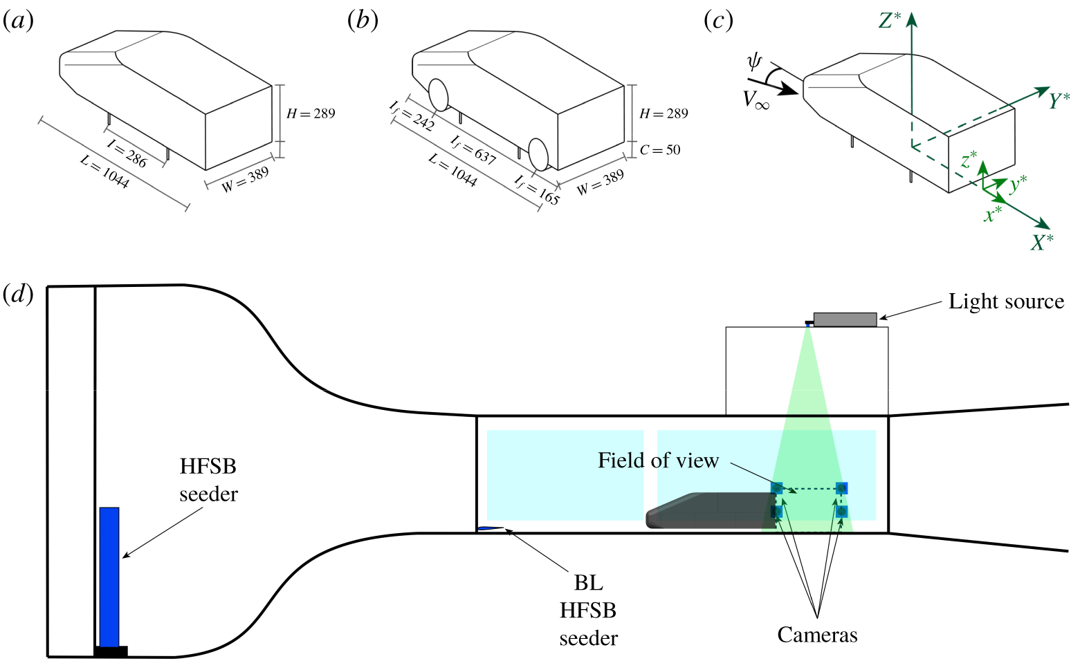
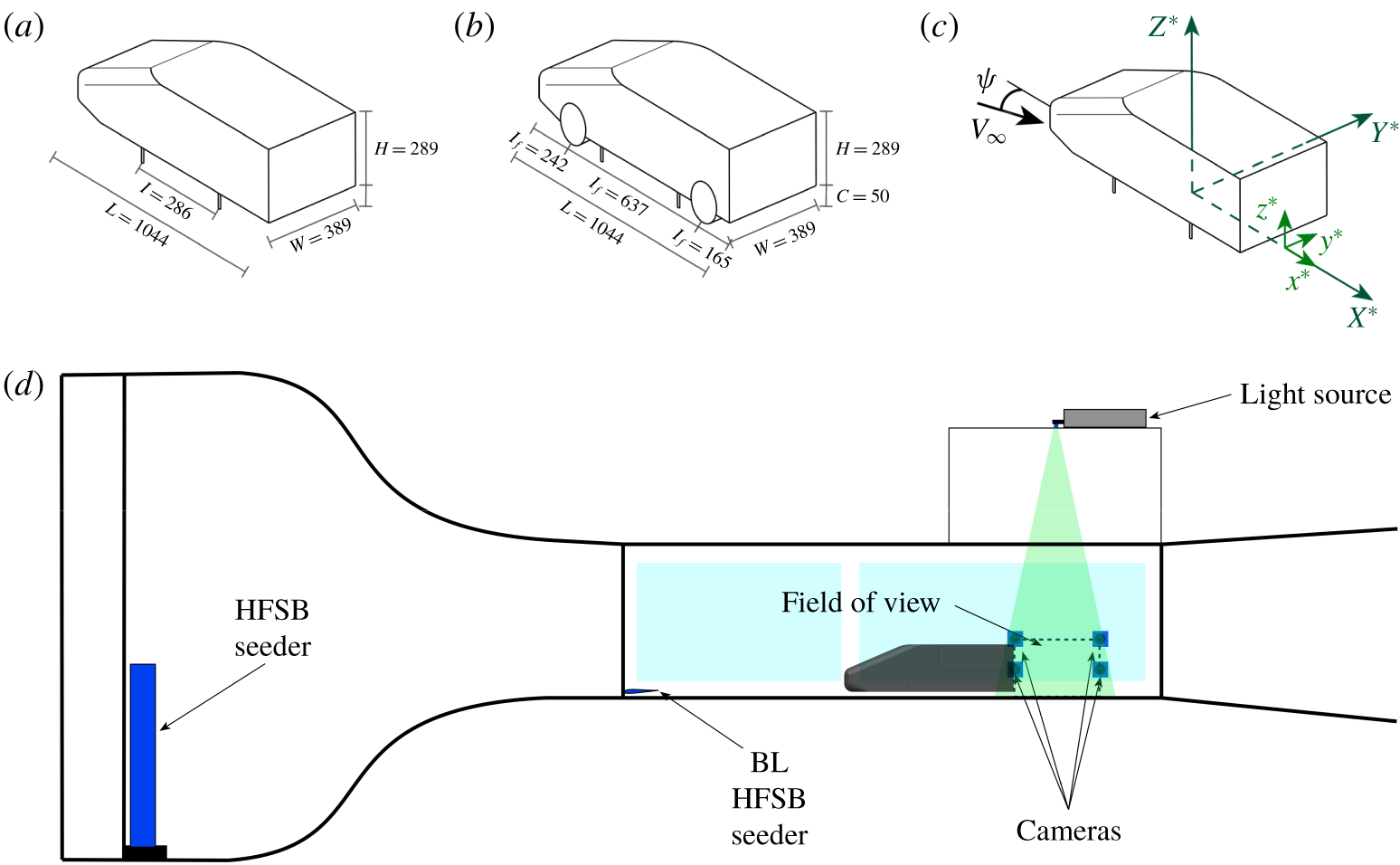
Schematic representations of the Windsor body, herein considered in two different configurations: (a) model with no wheels; (b) model with (stationary) wheels. All dimensions are in millimetres. (c) Reference systems used in the present investigation:  $X^{\ast },Y^{\ast },Z^{\ast }$ refer to the body’s global reference system (defined according the SAE coordinate system (SAE 2010)) whereas
 $x^{\ast },y^{\ast },z^{\ast }$ denote the reference system centred with the model base, used for the presentation of the results. (d) Schematic representation of the TPIV set-up.
2.1 Model
The experiment was carried out using the Windsor body, already used, among others, by Perry et al. (Reference Perry, Pavia and Passmore2016b) and Pavia et al. (Reference Pavia, Passmore and Sardu2018). The model has an overall length  $L$ of 1044 mm, a width
 $W$ of 389 mm and a height
 $H$ of 289 mm. The dimensions make it approximately representative of a 1/4-scale passenger car.
In the present investigation two configurations have been considered: one with the simple model (‘no-wheel case’, figure 1a), similar to that employed in Perry et al. (Reference Perry, Pavia and Passmore2016b) and Pavia et al. (Reference Pavia, Passmore and Sardu2018), and one with the model equipped with four (stationary) wheels (‘wheel case’, figure 1b), similar to that used in Pavia & Passmore (Reference Pavia and Passmore2017) and Varney, Passmore & Gaylard (Reference Varney, Passmore and Gaylard2018). Each wheel has an external diameter  $D_{w}$ of 150 mm and a maximum width of
 $W_{w}$ of 55 mm. The front axle is located 280 mm upstream of the centre of the model while the rear axle is 357 mm downstream of the same point, resulting in a wheelbase of 637 mm.
For all tests, the ground clearance was set at 50 mm, corresponding to a normalised value ( $h^{\ast }=h/H$) of 0.173, with a tolerance of ± 0. 2° for the pitch angle (Pavia et al. Reference Pavia, Passmore and Gaylard2016). The contact between the wheels and the ground was represented with a machined scallop, 3 mm deep, located underneath each wheel.
In both cases (with and without wheels) the model was mounted via four pins (consisting of  $M8$ threaded bars placed longitudinally between the two axles) to a yaw drive system that allowed rotation of the model around its vertical axis (defined according the SAE coordinate system (SAE 2010), as shown in figure 1c) to change the aerodynamic yaw angle, with an accuracy of ± 0. 1°. In such a way, any asymmetry present in the experimental set-up that could prevent the development of a ‘fully’ bi-stable wake was removed (Evrard et al. Reference Evrard, Cadot, Herbert, Ricot, Vigneron and Délery2016).
For the presentation of the results, the coordinate system is located on the model centreline at the model base (i.e.  $x^{\ast }$ is the back of the model), on the ground plane. The
 $x^{\ast }$ axis is aligned with the flow in the streamwise direction, the
 $z^{\ast }$ axis is vertical, positive upwards, and the
 $y^{\ast }$ axis follows a right-handed coordinate system (figure 1c). All quantities presented throughout the paper have been normalised using the model height
 $H$ as the reference length and the value of the free-stream velocity
 $V_{\infty }$; they are denoted with an asterisk. For the sake of clarity, the symbol ‘-’ is used to indicate time-averaged quantities whilst the subscript ‘LOM’ is used to denote quantities extracted from low-order models.
2.2 Test facility
The experiments were carried out in the Loughborough University large wind tunnel. The tunnel has an indraft configuration, with a test section of 1. 92 m × 1. 32 m × 3. 6 m ( $W_{T}\times H_{T}\times L_{T}$). The resulting blockage ratio was between 4.4 % and 4.7 %, depending on the model configuration (with no wheels or with wheels). The flow speed was set at
 $V_{\infty }=30~\text{m}~\text{s}^{-1}$, corresponding to a Reynolds number of
 $Re_{H}=5.78\times 10^{5}$ (based on the model height). In empty conditions the free-stream turbulence intensity is approximately 0.2 % and the flow uniformity ± 0. 4 % (Johl, Passmore & Render Reference Johl, Passmore and Render2004). Optical access in the test section was provided through glass sidewalls and a Perspex roof panel.
2.3 Tomographic PIV
Tomographic PIV (Scarano Reference Scarano2012) was employed to characterise the 3-D topology of the near-wake region. A volumetric field of view measuring 560 mm × 590 mm × 440 mm ( $L_{TPIV}\times W_{TPIV}\times H_{TPIV}$) was considered, based on the planar PIV data reported in Perry et al. (Reference Perry, Pavia and Passmore2016b), Pavia & Passmore (Reference Pavia and Passmore2017) and Pavia et al. (Reference Pavia, Passmore and Sardu2018). Four LaVision® cameras were used during the acquisition, two Imager Pro X 4M cameras (with a resolution of
 $2048\times 2048$ pixels and a pixel size of
 $7.4~\unicode[STIX]{x03BC}\text{m}^{2}$) and two sCMOS cameras (with a resolution of 2560 × 2160 pixels and a pixel size of 6. 5 μm2). Images were then reduced in software to a quarter of the original resolution because computer hardware limitations prevented analysis of the full-resolution dataset.
The cameras were mounted in a rectangular configuration (figure 1d), on a frame placed outside the tunnel test section. The aperture angle of the system was greater than 60° (Scarano Reference Scarano2012). Each camera was equipped with a Nikon® lens, with a focal length of 35 mm. The aperture was set to  $f_{\#}=8$ for all cameras in order to maintain the focus throughout the volume considered. The resulting depth of field was between ≈ 440 mm and ≈ 470 mm, depending on the camera. Calibration was carried out using a two-dimensional (2-D) calibration plate placed at five different locations within the volumetric field of view. The 3-D mapping functions obtained were then corrected by applying volume self-calibration (Wieneke Reference Wieneke2008).
To seed the flow, helium-filled soap bubbles with a diameter of 300 μm (Scarano et al. Reference Scarano, Ghaemi, Caridi, Bosbach, Dierksheide and Sciacchitano2015) were introduced from three wing-shaped rakes, each containing 10 nozzles producing up to 40 000 bubbles per second each. Two of the wings were mounted vertically at the start of the contraction whilst the third wing was mounted ≈ 30 mm from the floor at the start of the working section, to seed the model underbody (figure 1d). With the seeding system in place, a limited increase in the free-stream turbulence intensity is expected, although this has been shown to be relatively limited by Pavia et al. (Reference Pavia, Varney, Passmore and Almond2019b). The seeding arrangement allowed a stream-tube with a square cross-section of ≈ 400 mm × 400 mm (in the test section) to be seeded. Approximately 25 000 bubbles were captured in each 2-D image, giving a particle density of about 0.02 particles per pixel and a quality factor of  $Q\approx 0.95$ (Scarano Reference Scarano2012).
Illumination was provided by a 200 mJ Nd:YAG laser, mounted above the tunnel test section. The laser was expanded through a volume optic with a focal length of  $f_{\#}=-12$.
During each acquisition, 1000 statistically independent image pairs were recorded, at a sampling frequency of  $f_{s}=5~\text{Hz}$. This resulted in a total sampling time of 200 s corresponding to
 $t_{s}^{\ast }=2.076\times 10^{4}$ convective units. Data were processed using LaVision® DaVis 8.4.
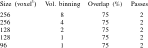
Image pre-processing was used to separate the light scattered by the particles from the background and mitigate the effects of spurious reflections, allowing a more accurate 3-D particle reconstruction (Elsinga et al. Reference Elsinga, Scarano, Wieneke and van Oudheusden2006). The FastMART algorithm, based on the work of Atkinson & Soria (Reference Atkinson and Soria2009), was used to reconstruct the position of the particles in 3-D space. The processing to produce the vector field was performed using a direct correlation multi-pass technique, starting with an interrogation window measuring 256 × 256 × 256 voxels and ending with a 96 × 96 × 96 voxel window (the intermediate processing steps are reported in table 1). Volume binning was employed in the first three passes in order to reduce the processing time (Discetti & Astarita Reference Discetti and Astarita2012), whilst the overlap between interrogation volumes was kept constant at 75 % for all passes. The velocity data obtained were then post-processed using a universal outlier detection technique to remove spurious vectors (Westerweel & Scarano Reference Westerweel and Scarano2005) as well as a smoothing function with a 3 × 3 × 3 spatial kernel. The resulting vector field is characterised by a resolution of 12 mm × 12 mm × 12 mm and a total vector count of approximately 87 000. The level of uncertainty in the mean velocity associated with each dataset has been estimated considering a 95 % confidence level (Perry et al. Reference Perry, Almond, Passmore and Littlewood2016a). This gives a value of 0.3 % for the free-stream velocity, increasing to over 5 % in proximity to the shear layers (Sellappan, McNally & Alvi Reference Sellappan, McNally and Alvi2018) where the fluctuations are greatest. A similar level of uncertainty is also observed at the corners of the volumetric field of view and close to the model base (for  $x^{\ast }\lessapprox 0.25$), as a consequence of the worsening of the signal-to-noise ratio. These regions of poor signal-to-noise ratio have been excluded from the analysis of the results, following the approach applied in Pavia et al. (Reference Pavia, Varney, Passmore and Almond2019b).
Settings used in the direct correlation algorithm employed for the processing of the TPIV data.

The most coherent unsteady features of the recorded data have been extracted by means of POD (Lumley Reference Lumley, Yaglom and Tatarski1967). A generic instantaneous velocity field  $\boldsymbol{V}(\boldsymbol{x},\boldsymbol{t})$ is decomposed as
 $$\begin{eqnarray}\boldsymbol{V}(\boldsymbol{x},t)=\overline{\boldsymbol{V}}(\boldsymbol{x})+\boldsymbol{v}^{\prime }(\boldsymbol{x},t)=\overline{\boldsymbol{V}}(\boldsymbol{x})+\mathop{\sum }_{n=1}^{N_{s}}\unicode[STIX]{x1D731}_{n}(\boldsymbol{x})a_{n}(t),\end{eqnarray}$$
where  $\overline{\boldsymbol{V}}(\boldsymbol{x})$ and
 $\boldsymbol{v}^{\prime }(\boldsymbol{x},t)$ represent, respectively, the time-averaged and fluctuating components of the considered field,
 $\unicode[STIX]{x1D731}_{n}(\boldsymbol{x})$ are the basis functions and
 $a_{n}(t)$ the related temporal coefficients (uncorrelated in time), whilst
 $N_{s}$ refers to the number of samples acquired. The basis functions
 $\unicode[STIX]{x1D731}_{n}(\boldsymbol{x})$ are determined solving an eigenvalue problem and the resulting eigenvalues, in descending order, are representative of the energy content
 $E$ of each mode. A low-order model can therefore be written as
 $$\begin{eqnarray}\boldsymbol{V}_{LOM}(\boldsymbol{x},t)\approx \overline{\boldsymbol{V}}(\boldsymbol{x})+\mathop{\sum }_{n=1}^{N_{m}}\unicode[STIX]{x1D731}_{n}(\boldsymbol{x})a_{n}(t),\end{eqnarray}$$
with  $N_{m}<N_{s}$. In the present case, the ‘snapshots method’ proposed by Sirovich (Reference Sirovich1987) has been applied, due to its higher computational efficiency when the temporal domain is smaller than the spatial domain. Examples of application of POD to TPIV data can be found in Ceglia et al. (Reference Ceglia, Discetti, Ianiro, Michaelis, Astarita and Cardone2014) and Pavia et al. (Reference Pavia, Varney, Passmore and Almond2019b). More information concerning the application of such a technique to fluid dynamic investigations is provided in Taira et al. (Reference Taira, Brunton, Dawson, Rowley, Colonius, McKeon, Schmidt, Gordeyev, Theofilis and Ukeiley2017).
3 No-wheel case: results and discussion
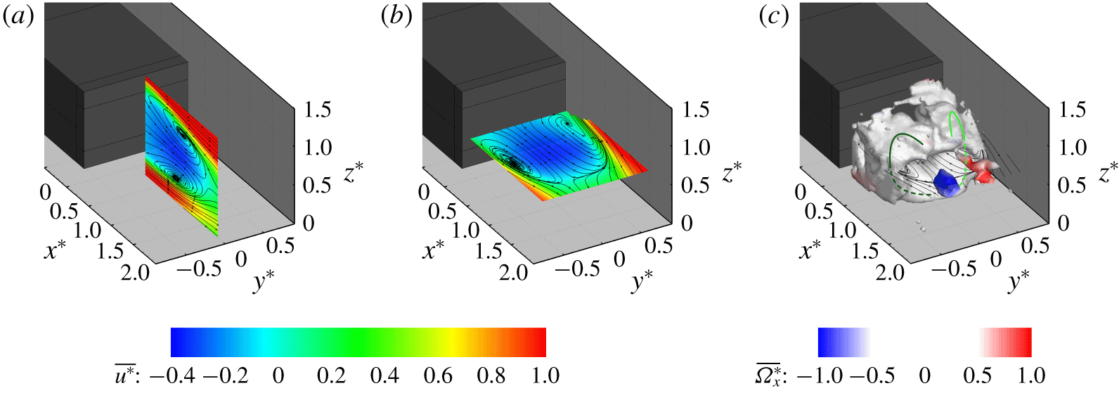
Time-averaged fields for the configuration with no wheels. Velocity fields captured along 2-D planes located at (a)  $y^{\ast }=0.00$ and (b)
 $z^{\ast }=0.67$. The planes are slices of the 3-D volume defined in § 2.3. All velocity fields are coloured according to the values of the axial component of the velocity
 $\overline{u^{\ast }}$; the streamlines refer to the in-plane components of the velocity. (c) Iso-surface of
 $\unicode[STIX]{x1D706}_{2}^{\ast }=-0.05$ (Jeong & Hussain Reference Jeong and Hussain1995) coloured by the values of the axial component of the vorticity
 $\overline{\unicode[STIX]{x1D6FA}_{x}^{\ast }}$. The 2-D streamlines from the plane located at
 $z^{\ast }=0.67$ are reported for reference. The green lines provide a schematic representation of the traces of the main vortical structures isolated in the wake. They are based on the continuity in the sign of the circulation as seen from the plane at
 $z^{\ast }=0.67$ (with light green denoting the clockwise direction and dark green the counterclockwise direction). The dashed lines denote the portions of the vortices located beneath the mid-horizontal plane (at
 $z^{\ast }=0.67$).

3.1 Time-averaged results
The time-averaged flow field obtained for the no-wheel configuration is presented in figure 2 and shows a good agreement with the wake topology reported in the literature for similar geometries (Grandemange et al. Reference Grandemange, Gohlke and Cadot2013b; Volpe et al. Reference Volpe, Devinant and Kourta2015). The near-wake topology features a good level of symmetry in both vertical and lateral directions evident in 2-D ‘slices’ of the volumetric domain (figure 2a,b). Similar results were obtained by Perry et al. (Reference Perry, Pavia and Passmore2016b) when performing planar PIV investigations in the near wake of the same body.
The toroidal shape reported by Perry et al. (Reference Perry, Almond, Passmore and Littlewood2016a) becomes evident when an iso-surface of  $\unicode[STIX]{x1D706}_{2}^{\ast }=-0.05$ (Jeong & Hussain Reference Jeong and Hussain1995) is considered (figure 2c). The torus joins the vortical structures isolated in the mid-vertical plane (matching those reported in Grandemange et al. (Reference Grandemange, Gohlke and Cadot2013b) and Perry et al. (Reference Perry, Pavia and Passmore2016b), as shown in figure 2a) with the structures seen in the mid-horizontal plane (figure 2b). It tends to become ‘thinner’ in proximity to the top shear layer, close to the model centreline, suggesting that it is actually the result of the merging of two separate ‘C’-shaped vortices, developing on either side of the model base (see green lines in figure 2c).
In the same figure, small coherent longitudinal structures, developing downstream of the wake closure and characterised by opposite values of the axial vorticity  $\overline{\unicode[STIX]{x1D6FA}_{x}^{\ast }}$, are also visible. These structures are reminiscent of the streamwise vortices isolated in the numerical simulations performed by Rouméas et al. (Reference Rouméas, Gilliéron and Kourta2009) as well as the experimental results reported by Grandemange et al. (Reference Grandemange, Gohlke and Cadot2013b) and Pavia et al. (Reference Pavia, Passmore and Sardu2018).
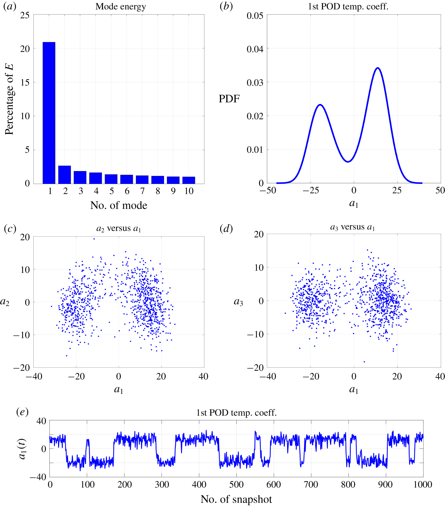
(a) Energy associated with the first 10 POD modes. (b) Probability density function of the first POD temporal mode (also known as lateral symmetry-breaking mode). (c) Scatter plot of the POD temporal coefficients associated with the symmetry-preserving mode ( $a_{2}(t)$) and the lateral symmetry-breaking mode (
 $a_{1}(t)$). (d) Scatter plot of the POD temporal coefficients associated with the vertical symmetry-breaking mode (
 $a_{3}(t)$) and the lateral symmetry-breaking mode (
 $a_{1}(t)$). (e) Temporal trend associated with the first POD temporal mode.

3.2 Unsteady results
Proper orthogonal decomposition was applied to the recorded dataset, with the aim of isolating the most coherent unsteady motions of the wake.
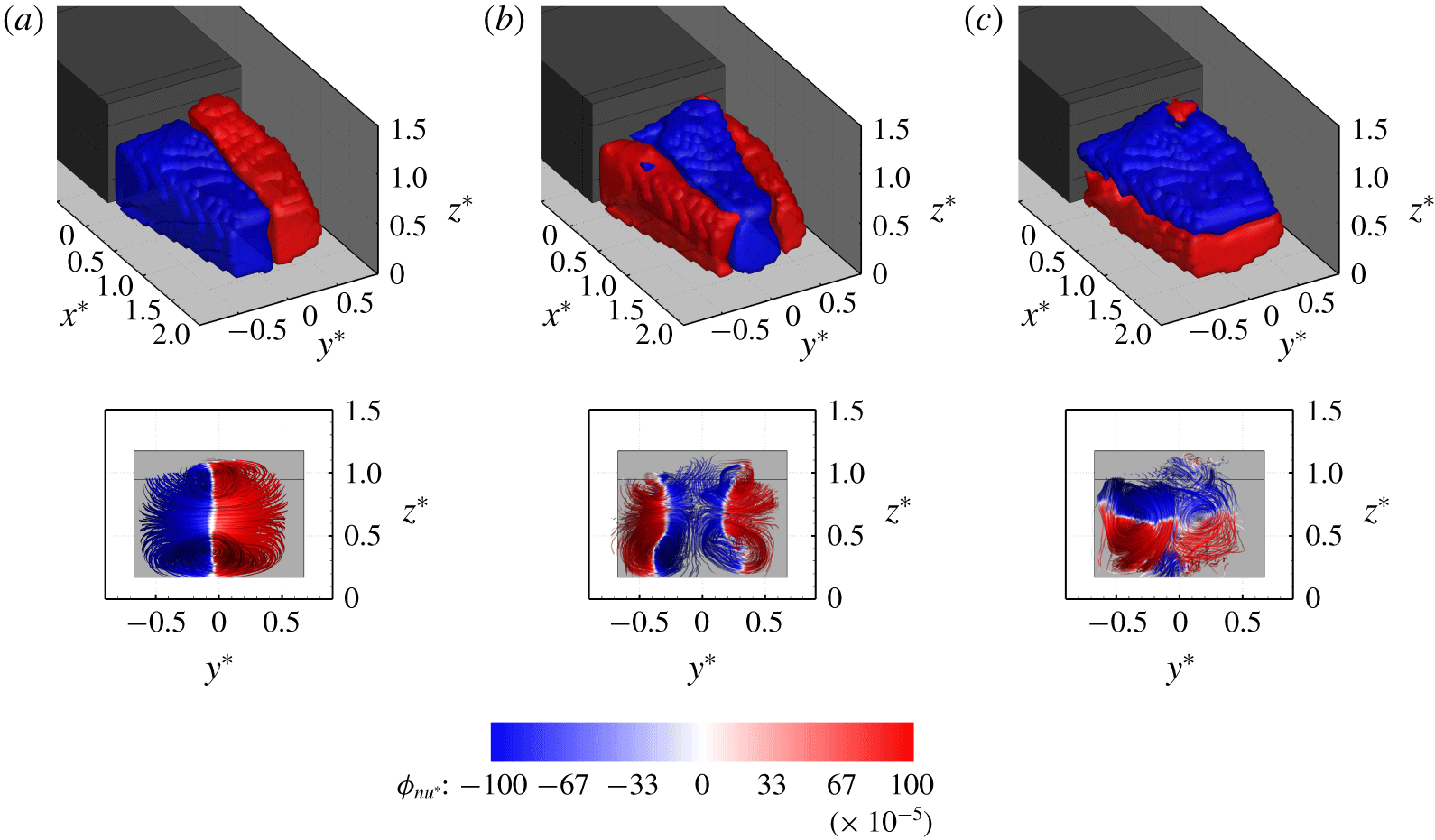
In the no-wheel case, the most energetic mode ( $n=1$ in 2.2) accounts for ≈ 21 % of the overall turbulent kinetic energy (figure 3a). This mode is associated with motions of the wake in both the lateral and longitudinal directions, as becomes clear when looking at the shape of the spatial function reported in figure 4(a). Two distinct regions, featuring, respectively, an excess and a deficit of streamwise momentum, can be seen in this figure. Each region extends for half of the wake cross-section, from the top shear layer to the bottom shear layer, covering the entire length of the rear recirculation. This results in a coherent motion that breaks the symmetry of the wake in the lateral direction, as also confirmed by the stream ribbons drawn in figure 4(a) (bottom row). In the same plot, most of the volumetric field of view is occupied by a horseshoe-like structure, aligned with the horizontal plane of symmetry of the model base. This structure is consistent with the lateral symmetry-breaking mode isolated by Pavia et al. (Reference Pavia, Passmore and Sardu2018) using stereoscopic PIV data.
Spatial functions of the first (a), second (b) and third (c) POD modes extracted from the TPIV dataset recorded for the no-wheel case. Top row: iso-surfaces of  $\unicode[STIX]{x1D719}_{n_{u^{\ast }}}=\pm 1\times 10^{-3}$, with
 $\unicode[STIX]{x1D719}_{n_{u^{\ast }}}$ denoting the axial component of the spatial mode
 $\unicode[STIX]{x1D6F7}_{n}$ defined in § 2.3; bottom row: stream ribbons drawn using the three components of
 $\unicode[STIX]{x1D6F7}_{n}$ (
 $\unicode[STIX]{x1D719}_{n_{u^{\ast }}}$,
 $\unicode[STIX]{x1D719}_{n_{v^{\ast }}}$,
 $\unicode[STIX]{x1D719}_{n_{w^{\ast }}}$). The ribbons are seen from a point downstream of the wake closure, looking upstream towards the base. The iso-surfaces and the stream ribbons are coloured according to the values of
 $\unicode[STIX]{x1D719}_{n_{u^{\ast }}}$.

Evidence of the existence of a strong bi-stable behaviour (Grandemange et al. Reference Grandemange, Gohlke and Cadot2013b) is provided by the step trend observed in the evolution of the temporal coefficient associated with the same POD mode ( $a_{1}(t)$ in (2.2)). As shown in figure 3(e),
 $a_{1}(t)$ tends to randomly switch between positive and negative, almost constant, values as a result of the existence of two different states. The switch between these two states is not periodic, as the wake can persist in a certain condition for any time interval ranging from less than
 $1$ s to more than
 $10$ s. This is similar to the trend isolated in the pressure signal recorded on the base of similarly shaped bodies by Volpe et al. (Reference Volpe, Devinant and Kourta2015) and Pavia et al. (Reference Pavia, Passmore and Gaylard2016). The two states are almost equally probable, as shown by the probability density function obtained for the values of
 $a_{1}(t)$, reported in figure 3(b). The fact that in the case considered here one of the states is slightly more probable has to be ascribed to the presence of some residual asymmetries in the experimental set-up (as in Evrard et al. (Reference Evrard, Cadot, Herbert, Ricot, Vigneron and Délery2016) and Pavia et al. (Reference Pavia, Passmore and Varney2019a)). The effect of this is evident in the values of the probability density function in figure 3(b), and is also visible in the time-averaged flow field presented in figure 2. In addition, in figure 3(b) the values of
 $a_{1}(t)$ associated with the most probable states are not exactly the opposite of each other (as one might expect). This is a consequence of the application of POD decomposition to an experimental dataset characterised by a very slow convergence. Nevertheless, it has been decided to avoid any ‘a posteriori’ re-symmetrisation of the data, as the ‘asymmetry’ was deemed to be not big enough to compromise any ‘general’ conclusion to be drawn from the present investigation.
The ability of the TPIV set-up to accurately capture the most energetic wake dynamics is further confirmed by the topology of the spatial functions obtained for the second and third POD modes, which closely resemble those reported in Pavia et al. (Reference Pavia, Passmore and Sardu2018). The second mode appears to be linked to axial motions of the near wake with opposite sign between the centre of the base and the lateral trailing edges (figure 4b). The stream ribbons reveal the existence of four vortex-like structures that preserve the symmetry of the wake in both vertical and lateral directions, justifying the appellative of symmetry-preserving mode (Pavia et al. Reference Pavia, Passmore and Sardu2018, Reference Pavia, Passmore and Varney2019a). The topology of the spatial function obtained for the third mode is more similar to that seen for the first mode; however, it appears to be associated with motion that breaks the symmetry of the wake in the vertical direction, as the horseshoe-like structure is aligned with the vertical plane of symmetry of the model base (figure 4c).
A good level of agreement between the TPIV data and the results presented using other methods is also found when looking at the relationship between the temporal coefficients associated with the latter modes and  $a_{1}(t)$. Pavia et al. (Reference Pavia, Passmore and Sardu2018) described a peculiar pattern in the scatter plot obtained from the values of the first two temporal coefficients (figure 3c) whereby
 $a_{2}(t)$ is observed to reach its highest positive values only when the symmetry of the wake is restored (
 $a_{1}(t)\rightarrow 0$). In the same conditions, no preferential direction is seen here in the distribution of the points associated with scatter plots of the temporal coefficients associated with the lateral symmetry-breaking mode and the vertical symmetry-breaking mode (figure 3d).
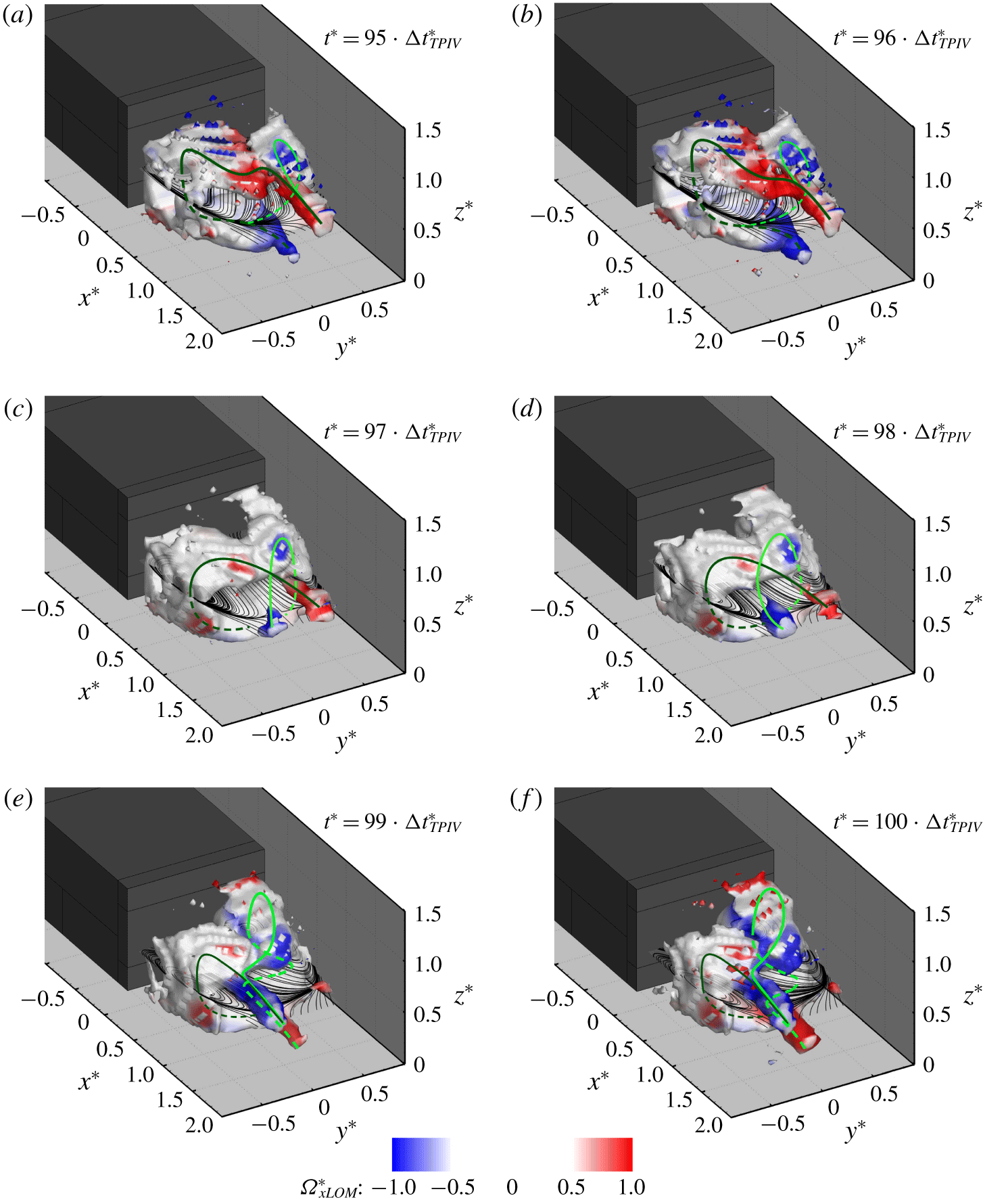
Temporal evolution of the wake’s recirculation. Results obtained combining the time-averaged field with the first POD mode. The most coherent structures are visualised by iso-surfaces of  $\unicode[STIX]{x1D706}_{2}^{\ast }=-0.05$ (Jeong & Hussain Reference Jeong and Hussain1995) coloured by the values of the axial component of the vorticity
 $\unicode[STIX]{x1D6FA}_{xLOM}^{\ast }$. The 2-D streamlines drawn on a horizontal plane centred with the model base (at
 $z^{\ast }=0.67$) are also reported. The green lines provide a schematic representation of the traces of the main vortical structures isolated in the wake, based on the continuity in the sign of the circulation as seen from the plane at
 $z^{\ast }=0.67$ (with light green denoting the clockwise direction and dark green the counterclockwise direction). The dashed lines denote the portions of the vortices located beneath the mid-horizontal plane (at
 $z^{\ast }=0.67$). For more information on the unsteady evolution of the wake, see supplementary movie 1.

More insights into the unsteady evolution of the near wake are provided by the low-order model built by combining the time-averaged field and the first POD mode, according to (2.2) (having considered  $N_{m}=1$). The results are presented in figure 5 (for six consecutive snapshots) and in supplementary movie 1 available at https://doi.org/10.1017/jfm.2020.71. Two distinct lateral symmetry-breaking states are captured: an L-state (figure 5a,b) and an R-state (figure 5e,f) depending on the position of the portion of the vortex filament closest to the base. As shown by the iso-surfaces of
 $\unicode[STIX]{x1D706}_{2}^{\ast }=-0.05$, each state is characterised by the presence of a vortical structure that stems from one of the model’s vertical trailing edges and then bends towards the opposite edge while extending downstream, terminating into one or two ‘tails’ aligned with the onset flow. This confirms the existence of the vortical structure initially described as a ‘horseshoe vortex’ by Evrard et al. (Reference Evrard, Cadot, Herbert, Ricot, Vigneron and Délery2016) and later as a ‘hairpin vortex’ by Pavia et al. (Reference Pavia, Passmore and Sardu2018). Indeed, the experimental evidence collected in the present investigation seems to confirm the latter model, as the ‘tails’ of the vortex are seen to ‘bend’ quite aggressively while extending downstream and they do not appear to have the same ‘strength’. The lower ‘tail’ is seen to alternately appear and disappear as the two sides of the hairpin vortex are continuously ‘stretched’ and ‘squeezed’ in the streamwise direction, as shown in supplementary movie 1. This may also be linked to the vortex shedding described in Grandemange et al. (Reference Grandemange, Gohlke and Cadot2013b), Volpe et al. (Reference Volpe, Devinant and Kourta2015), Pavia et al. (Reference Pavia, Passmore and Sardu2018) and Dalla Longa et al. (Reference Dalla Longa, Evstafyeva and Morgans2019), although time-resolved data are needed to confirm such a hypothesis.
By taking into account the continuity in the sign of the circulation between the left-hand side and the right-hand side of the model, it becomes clear that each hairpin vortex is indeed the result of the joining of two separate vortical structures. These structures present analogies with the ‘C-shaped’ horseshoe vortices featured in the model proposed by Perry et al. (Reference Perry, Pavia and Passmore2016b). Supplementary movie 1 shows that the bi-stable mode is a consequence of the unsteady interaction between these two structures. The lateral symmetry of the wake is broken every time one of the two vortices expands at the expense of the structure acting on the opposite side of the model. This in turn is moved further downstream of the base and is ‘squeezed’ against the nearby shear layer, assuming the characteristic elliptical cross-section often reported in the literature (Grandemange et al. Reference Grandemange, Gohlke and Cadot2013b; Volpe et al. Reference Volpe, Devinant and Kourta2015). The smaller structure, however, is still ‘strong’ enough to affect the larger vortex. This is highlighted by the abrupt change observed in the orientation of the ‘tails’ of the larger vortex as they approach the smaller structure (characterised by circulation of opposite sign). In the same conditions, the cross-sectional area of the iso-surface of  $\unicode[STIX]{x1D706}_{2}^{\ast }=-0.05$ bounding the ‘tails’ is also reduced, suggesting a weakening of the vortical structure.
A toroidal shape, similar to that reported for the time-averaged flow field, is observed during the switch between bi-stable states, when the lateral symmetry of the wake is temporarily restored (figure 5c,d), resulting in a symmetry-preserving state (Pavia et al. Reference Pavia, Passmore and Sardu2018). Even in this case, however, the presence of protrusions on the iso-surface of  $\unicode[STIX]{x1D706}_{2}^{\ast }=-0.05$ featuring relatively high values of axial vorticity suggests that the torus is the result of the joining of two transverse vortices developing on either side of the model. This would match the topology of the base pressure distribution reported by Pavia et al. (Reference Pavia, Passmore and Sardu2018) when analysing the switch between bi-stable states. In that case, the pressure distribution over the model’s rearward facing surfaces was reported to switch from a laterally asymmetric topology to a more symmetric shape, featuring two regions of low pressure extending vertically on either side of the base, separated by a ‘high-pressure’ region located at the centre.
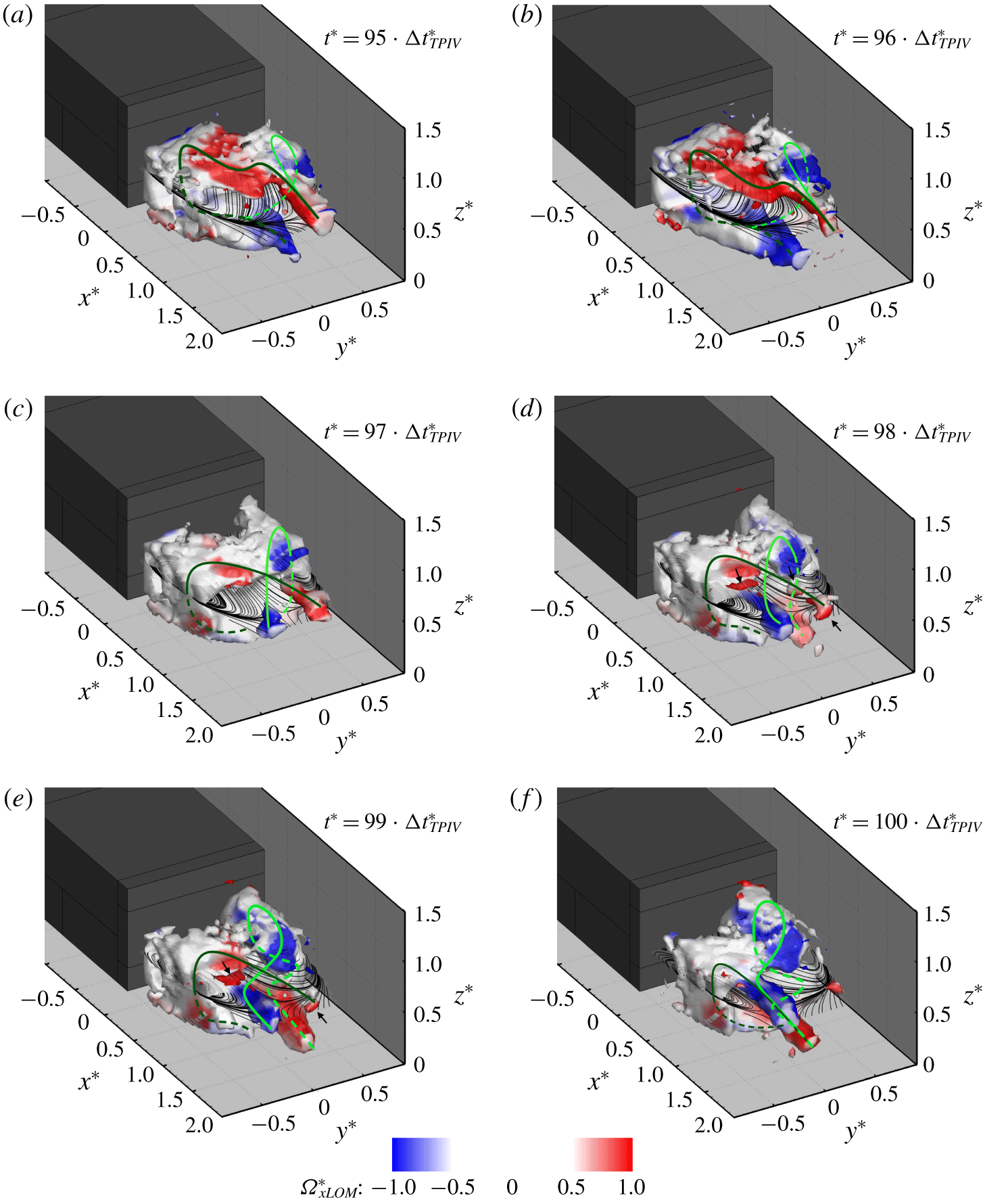
The nature of the symmetry-preserving state becomes clearer when the second POD mode is added to the reconstructed flow field (therefore  $N_{m}=2$ in (2.2)). The results are presented in figure 6 and supplementary movie 2. When in one of the symmetry-breaking states, the results are unchanged from figure 5, but significant differences can be observed during the transition between the two asymmetric states (or more generally every time the symmetry in the lateral direction is restored), as evident from figure 6. Figure 6(c–e) shows that a symmetry-preserving state is seen every time the two horseshoe vortices reach a condition of equal strength. The mutual interaction between the two vortices is such that both structures are moved away from the model base and pressed against the nearby shear layer. The increased separation between the cores of the wake vortices and the base has been found to be at the origin of the drag reduction observed in these conditions (Pavia et al. Reference Pavia, Passmore and Sardu2018). As each vortex bends towards the opposite side of the model while extending downstream, its ‘tails’ are seen to break up into smaller structures by the action of the second vortex (see arrows in figure 6d,e). This may also explain the presence of the longitudinal vortices seen in the time-averaged flow field, downstream of the wake closure (at
 $x^{\ast }\approx 1.5$, as shown in figure 2c), as these structures are the leftovers of the ‘tails’ of the horseshoe vortices as they ‘collide’ with each other.
Although the two vortices seem to intersect in proximity to the wake closure, their interaction appears to start further upstream, at  $x^{\ast }\approx 0.75$, explaining the results obtained by Grandemange et al. (Reference Grandemange, Gohlke and Cadot2014) when perturbing the wake downstream of a similarly shaped body with a small vertical control cylinder. In that case, the control cylinder was reported to stabilise the wake in a lateral symmetry-preserving state only when located in the mid-vertical plane, at
 $x^{\ast }=0.71$, which the results shown here indicate to be just upstream of the location where the two transverse vortices start to interact with each other. The perturbation generated by the wake forming downstream of the control cylinder may have been strong enough to spoil the interaction between the transverse vortices, preventing therefore the formation of the hairpin vortex previously described. However, additional work is needed to confirm this conjecture.
Temporal evolution of the wake’s recirculation. Results obtained combining the time-averaged field with the first two POD modes. The most coherent structures are visualised by iso-surfaces of  $\unicode[STIX]{x1D706}_{2}^{\ast }=-0.05$ (Jeong & Hussain Reference Jeong and Hussain1995) coloured by the values of the axial component of the vorticity
 $\unicode[STIX]{x1D6FA}_{xLOM}^{\ast }$. The 2-D streamlines drawn on a horizontal plane centred with the model base (at
 $z^{\ast }=0.67$) are also reported. The green lines provide a schematic representation of the traces of the main vortical structures isolated in the wake, based on the continuity in the sign of the circulation as seen from the plane at
 $z^{\ast }=0.67$ (with light green denoting the clockwise direction and dark green the counterclockwise direction). The dashed lines denote the portions of the vortices located beneath the mid-horizontal plane (at
 $z^{\ast }=0.67$). For more information on the unsteady evolution of the wake, see supplementary movie 2.

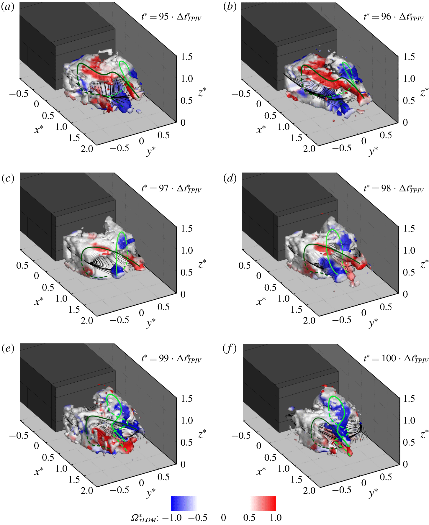
Temporal evolution of the wake’s recirculation. Results obtained combining the time-averaged field with the first three POD modes. The most coherent structures are visualised by iso-surfaces of  $\unicode[STIX]{x1D706}_{2}^{\ast }=-0.05$ (Jeong & Hussain Reference Jeong and Hussain1995) coloured by the values of the axial component of the vorticity
 $\unicode[STIX]{x1D6FA}_{xLOM}^{\ast }$. The 2-D streamlines drawn on a horizontal plane centred with the model base (at
 $z^{\ast }=0.67$) are also reported. The green lines provide a schematic representation of the traces of the main vortical structures isolated in the wake, based on the continuity in the sign of the circulation as seen from the plane at
 $z^{\ast }=0.67$ (with light green denoting the clockwise direction and dark green the counterclockwise direction). The dashed lines denote the portions of the vortices located beneath the mid-horizontal plane (at
 $z^{\ast }=0.67$). For more information on the unsteady evolution of the wake, see supplementary movie 3.

Adding the third POD mode ( $N_{m}=3$ in (2.2)), which represents the vertical symmetry-breaking mode, provides further insights into the interactions between the two horseshoe vortices, as shown in figure 7 (for six consecutive snapshots) as well as in supplementary movie 3. Unlike the addition of the second mode, the third POD mode changes the topology of the symmetry-breaking states. The hairpin vortex previously isolated in such conditions now appears to be more prone to break up into smaller structures, as a consequence of the interactions with the surrounding shear layers (figure 7a,f). This seems to confirm the findings of Grandemange et al. (Reference Grandemange, Gohlke and Cadot2013b) and Lucas et al. (Reference Lucas, Cadot, Herbert, Parpais and Délery2017) concerning the nature of the vortex shedding observed past square-back geometries. A similar trend can also be seen when the lateral symmetry is temporarily restored. Sometimes, because of the action of this mode, large coherent structures become hardly recognisable during the transition between lateral symmetry-breaking states (figure 7e).
4 Wheel case: results and discussion
4.1 Time-averaged results
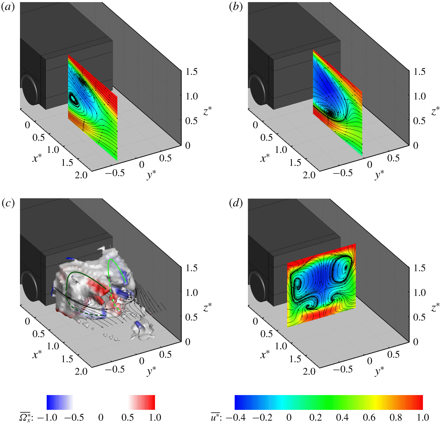
Time-averaged fields for the configuration with wheels. Velocity fields captured along 2-D planes located at (a)  $y^{\ast }=-0.34$, (b)
 $y^{\ast }=0.00$ and (d)
 $x^{\ast }=0.50$. The planes are slices of the 3-D volume defined in § 2.3. All velocity fields are coloured according to the values of the axial component of the velocity
 $\overline{u^{\ast }}$; the streamlines refer to the in-plane components of the velocity. (c) Iso-surface of
 $\unicode[STIX]{x1D706}_{2}^{\ast }=-0.05$ (Jeong & Hussain Reference Jeong and Hussain1995) coloured by the values of the axial component of the vorticity
 $\overline{\unicode[STIX]{x1D6FA}_{x}^{\ast }}$. The 2-D streamlines from the plane located at
 $z^{\ast }=0.67$ are reported for reference. The green lines provide a schematic representation of the traces of the main vortical structures isolated in the wake, based on the continuity in the sign of the circulation as seen from the plane at
 $z^{\ast }=0.67$. The dashed lines denote the portions of the vortices located beneath the mid-horizontal plane (at
 $z^{\ast }=0.67$).

The torus seen in the no-wheel case appears to be heavily deformed when wheels are added to the model (figure 8c). Four ‘protrusions’ (two on either side of the base) become clearly visible when considering the iso-surface of  $\unicode[STIX]{x1D706}_{2}^{\ast }=-0.05$. This suggests the presence of two horseshoe-like vortices aligned with each of the vertical edges of the model. These structures tend to get closer to each other in proximity to the bottom trailing edge, as they are ‘pushed’ towards the model centreline by the in-wash generated by the wake of the rear wheels (figure 8d). The existence of the two horseshoe-like structures agrees with the findings of Pavia & Passmore (Reference Pavia and Passmore2017), who reported the presence of two pairs of counter-rotating vortices in stereoscopic PIV measurements on a cross-plane located at
 $x^{\ast }=0.50$ downstream of the same model, confirming the correlation between planar and tomographic PIV measurements.
The accuracy of the TPIV system is also confirmed when comparing the time-averaged velocity fields reported in figure 8(a,b) with the 2-D PIV planes reported in Pavia (Reference Pavia2019) (having considered in this case the plane at  $y^{\ast }=-0.34$ rather than the plane at
 $y^{\ast }=0.34$ for easier visualisation of the results). In both cases the near-wake topology appears to be dominated by the bottom recirculation, which is seen to increase in size at the expense of the upper one resulting in the loss of vertical symmetry. The same recirculation also moves upstream, resulting in a reduction of the length of the entire wake compared to the no-wheels configuration, with the free stagnation point moved from
 $x^{\ast }\approx 1.5$ to
 $x^{\ast }\approx 1.3$. This explains the decrease in static pressure reported in the corresponding regions of the base by Pavia & Passmore (Reference Pavia and Passmore2017). The loss of symmetry in the vertical direction is also evident on the plane at
 $y^{\ast }=0.00$ (figure 8b). Unlike that seen in the PIV results reported in Pavia (Reference Pavia2019), however, no recirculation can be observed close to the top shear layer in the TPIV results, arguably because it is not resolved when using larger interrogation windows when processing the TPIV data (see § 2.3).
4.2 Unsteady results
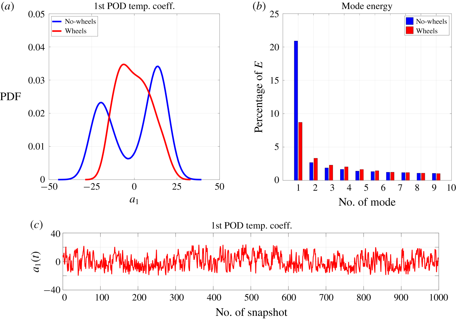
(a) Probability density function of the first POD temporal mode (also known as lateral symmetry-breaking mode). (b) Energy associated with the first 10 POD modes. (c) Temporal trend associated with the first POD temporal mode.

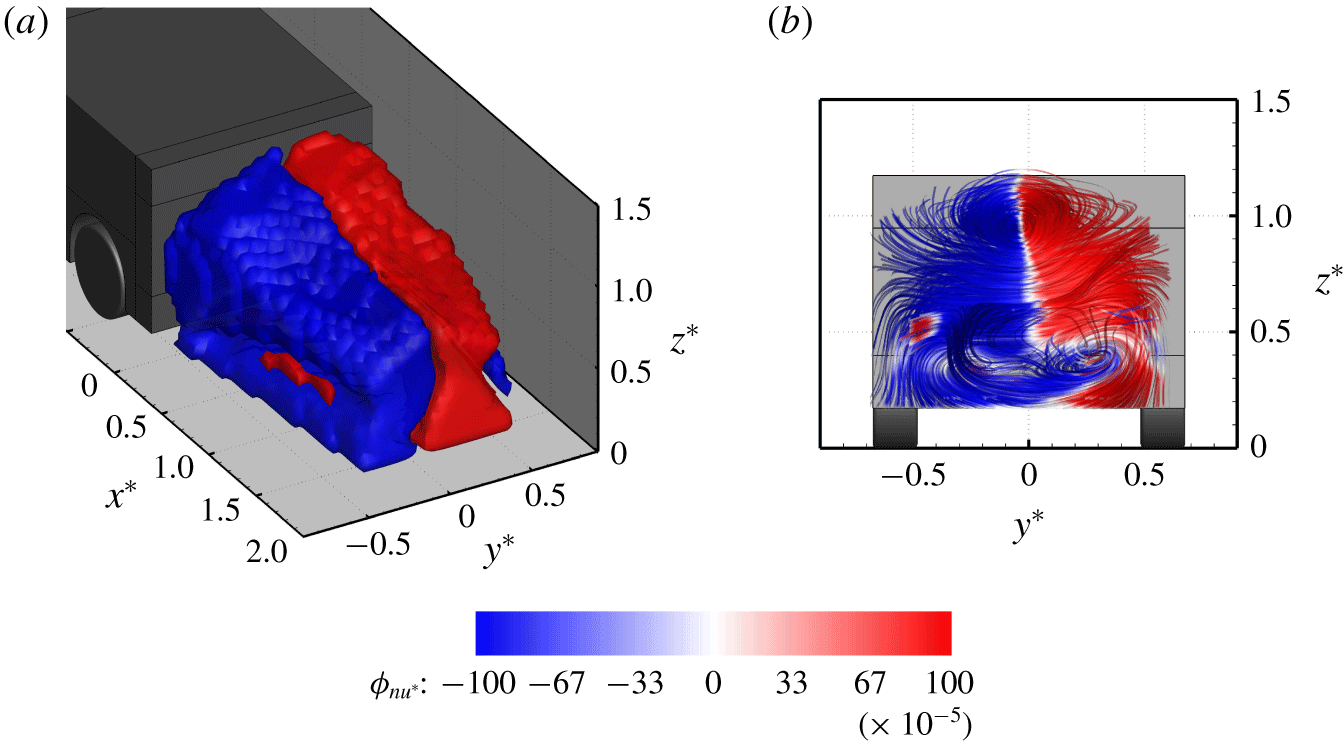
Spatial functions of the first POD mode extracted from the TPIV dataset recorded for the wheel case. (a) Iso-surfaces of  $\unicode[STIX]{x1D719}_{n_{u^{\ast }}}=\pm 1\times 10^{-3}$, with
 $\unicode[STIX]{x1D719}_{n_{u^{\ast }}}$ denoting the axial component of the spatial mode
 $\unicode[STIX]{x1D6F7}_{n}$ defined in § 2.3. (b) Stream ribbons drawn using the three components of
 $\unicode[STIX]{x1D6F7}_{n}$ (
 $\unicode[STIX]{x1D719}_{n_{u^{\ast }}}$,
 $\unicode[STIX]{x1D719}_{n_{v^{\ast }}}$,
 $\unicode[STIX]{x1D719}_{n_{w^{\ast }}}$). The ribbons are seen from a point downstream of the wake closure, looking upstream towards the base.The iso-surfaces and the stream ribbons are coloured according to the values of
 $\unicode[STIX]{x1D719}_{n_{u^{\ast }}}$.

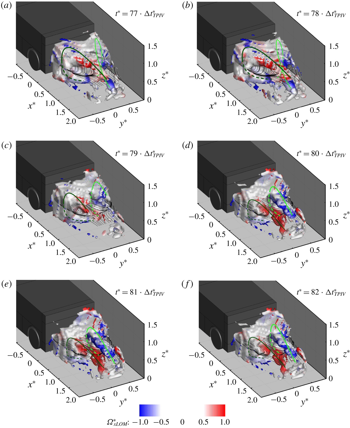
Temporal evolution of the wake’s recirculation in the wheel case. Results obtained combining the time-averaged field with the first POD mode. The most coherent structures are visualised by iso-surfaces of  $\unicode[STIX]{x1D706}_{2}^{\ast }=-0.05$ (Jeong & Hussain Reference Jeong and Hussain1995) coloured by the values of the axial component of the vorticity
 $\tilde{\unicode[STIX]{x1D6FA}}_{xLOM}^{\ast }$. The 2-D streamlines drawn on a horizontal plane centred with the model base (at
 $z^{\ast }=0.67$) are also reported. The green lines provide a schematic representation of the traces of the main vortical structures isolated in the wake, based on the continuity in the sign of the circulation as seen from the plane at
 $z^{\ast }=0.67$. The dashed lines denote the portions of the vortices located beneath the mid-horizontal plane (at
 $z^{\ast }=0.67$). For more information on the unsteady evolution of the wake, see supplementary movie 4.

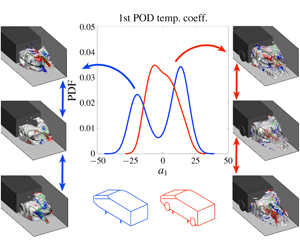
The bi-modal distribution obtained for the no-wheel configuration disappears when wheels are added to the model, although the peak is quite broad in the probability density function obtained for the values of  $a_{1}(t)$ (figure 9a). Nevertheless, the shape of the spatial function associated with the first POD mode preserves the left-to-right anti-symmetry seen in the no-wheel case (figure 10a). This, combined with the fact that
 $a_{1}(t)$ is seen to oscillate in time around zero (figure 9c), suggests that a certain degree of mobility in the lateral direction is still present in the wake, in agreement with the results reported in Pavia & Passmore (Reference Pavia and Passmore2017).
Changes in the shape of the spatial function associated with the first POD mode can be observed between the no-wheel and wheel configurations (figures 4a and 10). Although in both cases the regions with opposite fluctuation of streamwise velocity extend for the entire length of the rear recirculation, some differences can be seen close to the bottom trailing edge of the model. In the wheel case, the portion of the fluid domain with the highest excess/deficit of streamwise momentum appears to be ‘squeezed’ towards the model’s centreline by the wake downstream of each rear wheel (figure 10a). At the same time a change in topology is seen when stream ribbons are drawn in the same domain (figure 10b). The horseshoe-like structure reminiscent of the lateral symmetry-breaking mode isolated in Pavia et al. (Reference Pavia, Passmore and Sardu2018) (figure 4a) is now replaced by a ‘three-vortex’ arrangement, following the split of the bottom ‘vortex’ into two smaller ‘structures’ (Pavia Reference Pavia2019).
For a square-back body with  $W/H>1$, Perry et al. (Reference Perry, Pavia and Passmore2016b) and Pavia et al. (Reference Pavia, Passmore and Varney2019a) showed that the switch between bi-stable states represents by far the main contribution to the energy content of the lateral symmetry-breaking POD mode and that a change in the energy level of such a mode can be used to determine the strengthening/weakening of this long-time instability. This is confirmed here, as an approximately 12 % drop is observed in the energy level of the first POD mode when wheels are added to the model (figure 9b). The weakening of the bi-stable lateral symmetry-breaking mode, following the loss of symmetry in the vertical direction, agrees also with the findings of Barros et al. (Reference Barros, Borée, Cadot, Spohn and Noack2017), Bonnavion & Cadot (Reference Bonnavion and Cadot2018) and Pavia et al. (Reference Pavia, Varney, Passmore and Almond2019b).
As for the no-wheel case (§ 3.2), additional information on the unsteady evolution of the near wake can be gathered by considering a low-order model limited to the most energetic POD modes, having considered in this case  $N_{m}=1$ in (2.2) for the sake of simplicity. The results, presented in figure 11 and supplementary movie 4, show that the dynamics of the near wake is dominated in this case by the alternating expansion and contraction of the upper ‘tail’ of the horseshoe vortices isolated in the time-averaged results for the wheel case (§ 4.1). As the ‘tail’ on one side increases in size and stretches in the streamwise direction, it ‘pushes’ the one on the opposite side towards the ground, resulting in the twisting of the entire wake. The same process is then repeated in the opposite direction, leading to the ‘swinging motion’ described in Pavia & Passmore (Reference Pavia and Passmore2017) and Pavia (Reference Pavia2019). This process is characterised by a much shorter time scale than that seen in the case of the switch between bi-stable states, in agreement with the trend seen in figure 9(c) for the first POD temporal coefficient. Pavia (Reference Pavia2019) linked this motion with the inflection point seen in the power spectral density of the pressure data recored over the model base at
 $St_{H}\approx 0.02$ (with
 $St_{H}$ denoting the Strouhal number based on the model height
 $H$). In the present investigation, this corresponds to a time scale of ≈ 0. 5 s.
The analysis in the wheel case has been limited to just the first POD mode since the higher-order modes (with  $n>1$) are essentially shear-layer modes, as pointed out in Pavia (Reference Pavia2019). Therefore, their contribution to the global dynamics of the wake is more limited whilst the uncertainty associated with them is higher, as already mentioned in § 2.3.
5 Summary and conclusions
In the present work, the unsteady wake of a simplified square-back vehicle, with and without wheels, has been investigated using large-scale TPIV.
In the no-wheel case, the time-averaged wake has been shown to feature a balanced toroidal shape, confirming the results of previous TPIV investigations (Perry et al. Reference Perry, Almond, Passmore and Littlewood2016a). However, analysis of the wake dynamics shows this to be a poor model of the wake structure.
Characterising the unsteady evolution of the near wake using POD has revealed the existence of a strong bi-stable behaviour (Grandemange et al. Reference Grandemange, Gohlke and Cadot2013b), where the wake switches between two lateral symmetry-breaking states. Each state has been shown to feature a characteristic hairpin vortex, for which the 3-D topology has been characterised for the first time with the support of three-component volumetric experimental data, confirming the topology proposed by Pavia et al. (Reference Pavia, Passmore and Sardu2018).
An in-depth analysis has revealed that this topology is the result of the merging of two separate horseshoe vortices, developing on either side of the model base and reminiscent of the ‘C’-shaped vortices conjectured by Perry et al. (Reference Perry, Pavia and Passmore2016b). This model fits with the ‘bi-stable domain’ defined by Grandemange et al. (Reference Grandemange, Gohlke and Cadot2013a), as these structures are seen to form in proximity to the shorter side of the model base.
During transition between the two asymmetric states the two horseshoe vortices reach a condition of equal strength. In this condition, their interaction with the model base becomes weaker, thereby reducing the drag (Pavia et al. Reference Pavia, Passmore and Sardu2018). Beyond the wake closure, the tails of these structures are responsible for the longitudinal vorticies seen in the time-averaged data (Rouméas et al. Reference Rouméas, Gilliéron and Kourta2009; Grandemange et al. Reference Grandemange, Gohlke and Cadot2013b).
The fact that bi-stability has been shown to be the result of the interactions of two separate structures confirms the conjecture by Cadot, Evrard & Pastur (Reference Cadot, Evrard and Pastur2015) (lately reinforced also by the results of the experimental investigations carried out by Varon et al. (Reference Varon, Eulalie, Edwige, Gilotte and Aider2017)) regarding the existence of similarities between the turbulent wake developing downstream of square-back geometries and other fluid dynamic phenomena, such as the von Karman swirling flows (de la Torre & Burguete Reference de la Torre and Burguete2007; Faranda et al. Reference Faranda, Sato, Saint-Michel, Wiertel, Padilla, Dubrulle and Daviaud2017).
The addition of wheels ‘locks’ the transverse vortices in place and the long-time bi-stable mode vanishes, replaced by a short-time swinging motion of the rear recirculation (Pavia & Passmore Reference Pavia and Passmore2017; Pavia Reference Pavia2019), triggered by the alternate expansion/contraction of the upper ‘vortex tails’.
The investigation has proven that TPIV is sufficiently mature to be used when characterising the topology of the time-averaged wake of a ground vehicle or assessing the sensitivity of the same wake to changes in the model geometry. The same technique has also been shown to provide useful insights into the unsteady evolution of the wake as a whole. This opens new avenues for ground vehicle aerodynamic research, especially in the case of highly 3-D flow fields, such as those seen in the case of vehicles at yaw (Varney et al. Reference Varney, Passmore and Gaylard2018).
Declaration of interests
The authors report no conflict of interest.
Supplementary movies
Supplementary movies are available at https://doi.org/10.1017/jfm.2020.71.