2.1 Real-gas equation of state

For analysis of compressible flow at very high pressures, corrections to the ideal-gas relations are needed in the supporting thermodynamics theory. Amongst other issues, many classical relations no longer apply in their original forms. In particular, adjustments are needed for the equations of state that describe density (or specific volume), enthalpy, and sound speed as functions of pressure, temperature and composition.

Poling et al. (Reference Poling, Prausnitz and O’Connell2001) presents several equation-of-state formulations, including the well-known cubic EoS by van der Waals, Peng and Robinson, and Redlich and Kwong, governing the compressibility factor $Z\equiv pv/(R_{u}T)=p/(\unicode[STIX]{x1D70C}RT)$ . Variations of the Redlich–Kwong EoS have been advanced by Chueh & Prausnitz (Reference Chueh and Prausnitz1967a ,Reference Chueh and Prausnitz b ) and by Soave (Reference Soave1972). For an ideal gas, $Z=1$ everywhere, while, for a real gas, it may vary with space and time. Like any EoS in a system together with conservation equations, the cubic equation presents molar specific volume $v$ or mass density $\unicode[STIX]{x1D70C}$ as an implicit function of pressure $p$ and temperature $T$ . In addition, an enthalpy departure function gives the difference between the enthalpy for the ideal gas and the enthalpy for the real gas at any given pressure and temperature. Essentially, there is a pair of state equations, one for density and another for enthalpy  $h$ . The developments proposed here may be done with any of these cubic EoS but only one is chosen here. In particular, the analysis proceeds with the Soave–Redlich–Kwong (SRK) cubic EoS, which is known for accuracy over a wide range of important applications. For example, Lapuerta & Agudelo (Reference Lapuerta, Ballesteros and Agudelo2006) compared several real-gas EoS with experimental results relevant to diesel engine combustion and showed that the SRK EoS gave the best agreement.

The SRK EoS for a single-component fluid is

(2.1) $$\begin{eqnarray}Z^{3}-Z^{2}+(A-B-B^{2})Z-AB=0,\end{eqnarray}$$

where

(2.2) $$\begin{eqnarray}\displaystyle & \displaystyle Z\equiv \frac{pv}{R_{u}T}=\frac{p}{\unicode[STIX]{x1D70C}RT}, & \displaystyle\end{eqnarray}$$

(2.3) $$\begin{eqnarray}\displaystyle & \displaystyle A\equiv \frac{ap}{(R_{u}T)^{2}}, & \displaystyle\end{eqnarray}$$

(2.4) $$\begin{eqnarray}\displaystyle & \displaystyle B\equiv \frac{bp}{R_{u}T}, & \displaystyle\end{eqnarray}$$

(2.5) $$\begin{eqnarray}\displaystyle & \displaystyle a\equiv 0.42748\frac{(R_{u}T_{c})^{2}}{p_{c}}[1+S(1-T_{r}^{0.5})]^{2}, & \displaystyle\end{eqnarray}$$

(2.6) $$\begin{eqnarray}\displaystyle & \displaystyle b\equiv 0.08664\frac{R_{u}T_{c}}{p_{c}}, & \displaystyle\end{eqnarray}$$

(2.7) $$\begin{eqnarray}\displaystyle & \displaystyle T_{r}\equiv \frac{T}{T_{c}}, & \displaystyle\end{eqnarray}$$

(2.8) $$\begin{eqnarray}\displaystyle & \displaystyle S\equiv 0.48508+1.5517\unicode[STIX]{x1D714}-0.15613\unicode[STIX]{x1D714}^{2}. & \displaystyle\end{eqnarray}$$

Here $R$ and $R_{u}$ are the specific and universal gas constants, respectively; and subscript $c$ denotes a thermodynamic critical value. The coefficients $a$ and $b$ (and therefore $A$ and $B$ ) relate, respectively, to intermolecular attraction and repulsion. The second and third constant coefficients in the polynomial for $S$ differ slightly from the original Soave (Reference Soave1972) values. They are updated values by Graboski & Daubert (Reference Graboski and Daubert1978), which were also used by Meng & Yang (Reference Meng and Yang2003). (A different functional form is recommended for hydrogen; while discussion of gases with differing mathematical description is omitted to avoid distraction from the main themes, the approach is easily extendable to consider them.) In the domain of pressure and temperature where both gas and liquid exist in equilibrium, there is a solution of (2.1) for each phase; thus, two different, physically meaningful $Z$ values can result. Since $p$ and $T$ are identical for each phase, the implication is that there are two values for the specific molar volumes $v_{g}$ and $v_{l}$ and thereby for the mass densities $\unicode[STIX]{x1D70C}_{g}=W/v_{g}$ and $\unicode[STIX]{x1D70C}_{l}=W/v_{l}$ ; where $W$ is the molar mass. A range of values is considered for $p$ and $T$ where only one phase exists and therefore only one interesting solution to the cubic equation exists (complex roots are ignored). At supercritical conditions, there are ranges of $p$ and $T$ where a compressible fluid exists without discontinuities in properties and may still be labelled as a gas. Thus, reference to $\unicode[STIX]{x1D70C}$ and other properties are made with the understanding they apply to a gas.

The properties for flows of gaseous mixtures are not calculated here; however, the extension for that situation is straightforward (Poling et al. Reference Poling, Prausnitz and O’Connell2001).

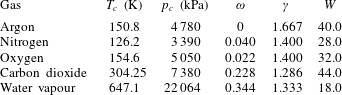
Table 1 presents critical temperature $T_{c}$ , critical pressure $p_{c}$ , acentric factor $\unicode[STIX]{x1D714}$ , ratio of specific heats for the ideal gas $\unicode[STIX]{x1D6FE}$ , and molecular mass $W$ for selected gases. Monatomic, diatomic and triatomic species are considered. In the calculations in the following sections, argon, nitrogen and carbon dioxide are analysed. Values of $\unicode[STIX]{x1D6FE}$ , $c_{p}$ and $c_{v}$ pertain only to the ideal-gas EoS. For example, as shown by (B 1), $c_{p}$ will not be the partial derivative of enthalpy with respect to temperature for a real gas. It will be that derivative only for an ideal gas and it retains only that meaning when used in the real-gas enthalpy relation.

Table 1.

Values for critical temperature, critical pressure, acentric factor and ratio of specific heats.

There is no obvious way to reduce the mathematical descriptions of different gases to a similar form for ease of calculation. For example, even if pressure and temperature are normalized, and $p/p_{c}$ and $T/T_{c}$ are treated, the gases differ significantly through three other parameters in table 1.

2.2 Linearized treatment of real-gas equation of state

The cubic EoS can be solved exactly for the compressibility factor $Z$ in terms of parameters $A$ and $B$ . Some 500 years ago, mathematicians S. del Ferro and N. Tartaglia obtained solutions for the cubic equation in a form involving cubic roots of functions formed as an algebraically elaborate collection of coefficients in the original equation. The exact solution is not useful in flow analysis. Firstly, the dependence of the coefficients of the cubic equation on unknown variables such as pressure, temperature and (for multicomponent flows) composition creates a higher-order system; i.e. there are couplings with other differential equations. Thereby, an iterative approach is required. Secondly, in a flow that develops in space and/or time, it is preferred to iterate about the solution at a prior time step or mesh point rather than returning to decide which of the cubic equation solutions to choose. The known additional computational challenges for real-gas, compressible-flow computation and the need for reliable approximations were addressed in § 1.2 with references to Colella & Glaz (Reference Colella and Glaz1985), Kouremenos (Reference Kouremenos1986), Drikakis & Tsangaris (Reference Drikakis and Tsangaris1993) and Arina (Reference Arina2004).

Approximations through perturbation expansions have been attempted. Tsien (Reference Tsien1946) used a linearization concept which differs from this work in several key features. The modern cubic equations were not available at that time; he used the van der Waals EoS where the parameter $a$ was a constant whereas the modern versions have $a(T)$ , i.e. a function of temperature $T$ , as shown by (2.8). Also, the important effects of internal energy and enthalpy departures from the ideal-gas behaviour were missing; among other things, there was no dependence of enthalpy or internal energy upon pressure. Tao (Reference Tao1955) used the Beattie-Bridgeman EoS and perturbation theory with six small parameters to describe the thermodynamics for normal shock analysis. Anand (Reference Anand2012) reports solutions for real-gas shock waves propagating at subsonic velocity. He uses an EoS with a repulsive molecular parameter but without an attractive molecular parameter. Glaister (Reference Glaister1988) and Guardone & Vigevano (Reference Guardone and Vigevano2002) discuss linearization of the numerical algorithms in Riemann problem solvers.

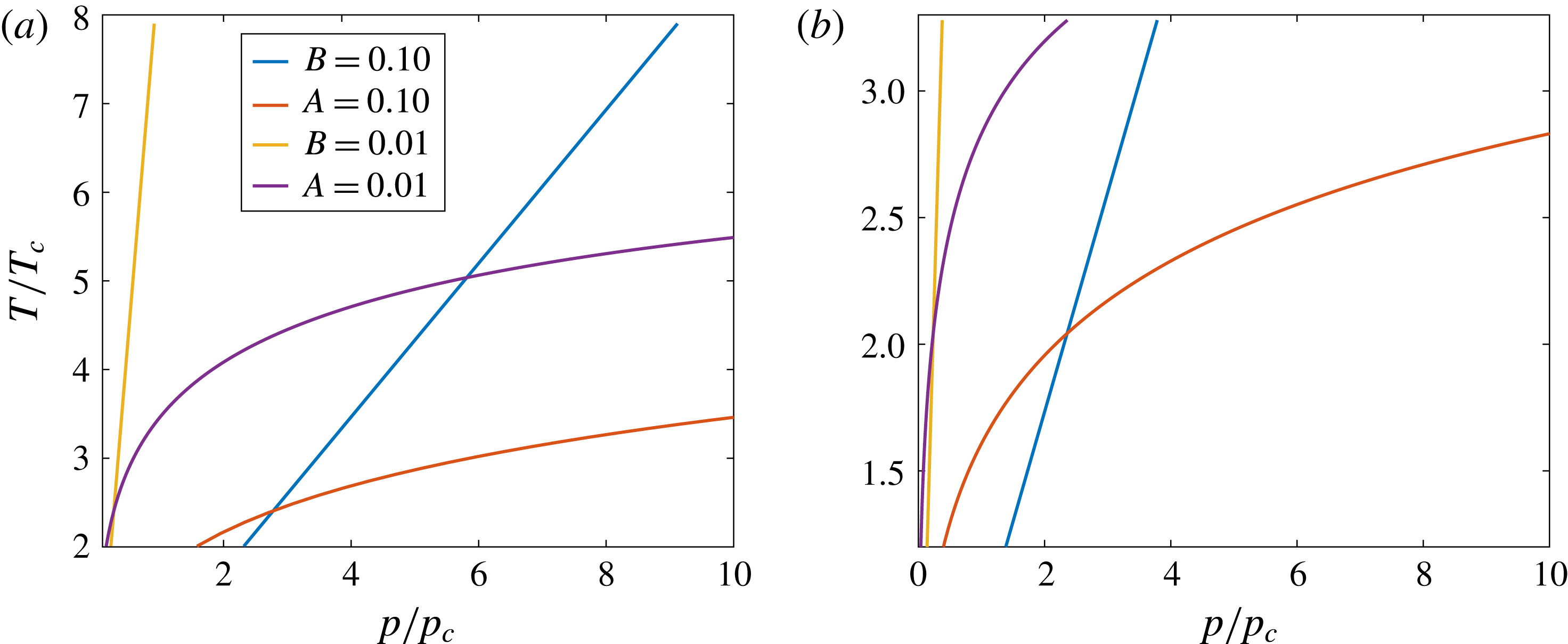
Here, it is shown that for a wide range of practical interest where the fluid temperature is well above the critical value, certain approximate solutions to the cubic EoS give sufficient accuracy and clarity of the physics. Often the parameters $A$ and $B$ have magnitudes substantially smaller than unity, making $Z-1$ also small in magnitude. As one example, consider an application by Jorda-Juanos & Sirignano (Reference Jorda-Juanos and Sirignano2016) where, for a mixture typical in combustion of methane, the temperature exceeds 400 K, and the parameters $z\equiv Z-1$ , $A$ and $B$ are small in magnitude. Specifically, they remain $O(10^{-1})$ or less at pressures up to 100 bar. Thereby, a linear perturbation expansion in the three parameters $z$ , $A$ and $B$ provides useful, accurate, simplified algorithms. In particular, neglecting squares and cubes of $z$ and products and squares of $A$ and $B$ , (2.1) can be simplified to

(2.9) $$\begin{eqnarray}\displaystyle Z\approx 1+B-A. & & \displaystyle\end{eqnarray}$$

The parameter $a$ and therefore $A$ represent the effects of intermolecular attraction; so, an increase in $A$ by itself would increase density at fixed temperature, pressure and composition. On the other hand, the parameter $b$ and therefore $B$ represent the effects of intermolecular repulsion; so, an increase in $B$ by itself at otherwise fixed conditions would decrease density. The linear form of the EoS given by (2.9) explains the impact of the molecular physics on the continuum properties in much clearer fashion than the original cubic EoS. Of course, in addition, it simplifies the flow analysis and carries the dependence on the molecular parameters in a much more informative fashion. The reasonable assumption is made that all flow variables are analytic in the fluid properties. (For the case with shock waves, we mean piecewise analytic.) And a small parameter never appears before the highest derivative. Thereby, the flow variables are calculated with accuracy to order of $A$ and $B$ and with error of order $A^{2}$ , $AB$ and  $B^{2}$ . In appendix A, it is shown that the accuracy of that approximation in (2.9) can be maintained over a substantial parameter domain of interest. While density depends simply on $B-A$ here, the enthalpy and sound speed depend on $A$ and $B$ in different ways as well as depending on derivatives of $a(T)$ introduced through the functions $A^{\prime }$ and $A^{\prime \prime }$ , which are defined in appendix B, where the real-gas enthalpy relation is presented.

If the linear perturbations in (2.9) are neglected, the ideal-gas equation, i.e.  $Z=1$ , is obtained. This linear form does not apply for two-phase domains or for the supercritical domain where a compressible-liquid behaviour occurs. The above-mentioned lower bound on temperature avoids these regions. At some temperatures and pressures, $Z-1$ might be small but $A$ and $B$ might not be sufficiently small to neglect higher-order terms in the cubic equation; thus, bounds on $A$ and $B$ individually are necessary here.

While other forms of the cubic EoS, including the original van der Waals equation and the more recent Peng–Robinson form of the cubic equation, differ from the Redlich–Kwong form presented here, they produce exactly the same linear approximation as given by (2.9). There is only a difference with the Peng–Robinson linearized version in the $S$ parameter, which affects the value of $A$ but not its order of magnitude. The van der Waals equation does not contain the added temperature dependence in the $a$ parameter. Consequently, the definition of $A$ in the linear version is different. In summary, our analysis here provides a template for linearization of the Peng–Robinson model and several other similar models.

The linear solution to the cubic equation reduces computational effort in flow-field calculations. In the context of the flow calculation, exact solution of the cubic equation requires an iterative process. The solution to a system of differential equations already requires iteration of some kind to get a well-converged solution as time is advanced at each step. If at each point in time and space another iteration were added within the finite-difference (or finite-volume) iteration, a substantial increase in computational resources would be needed.

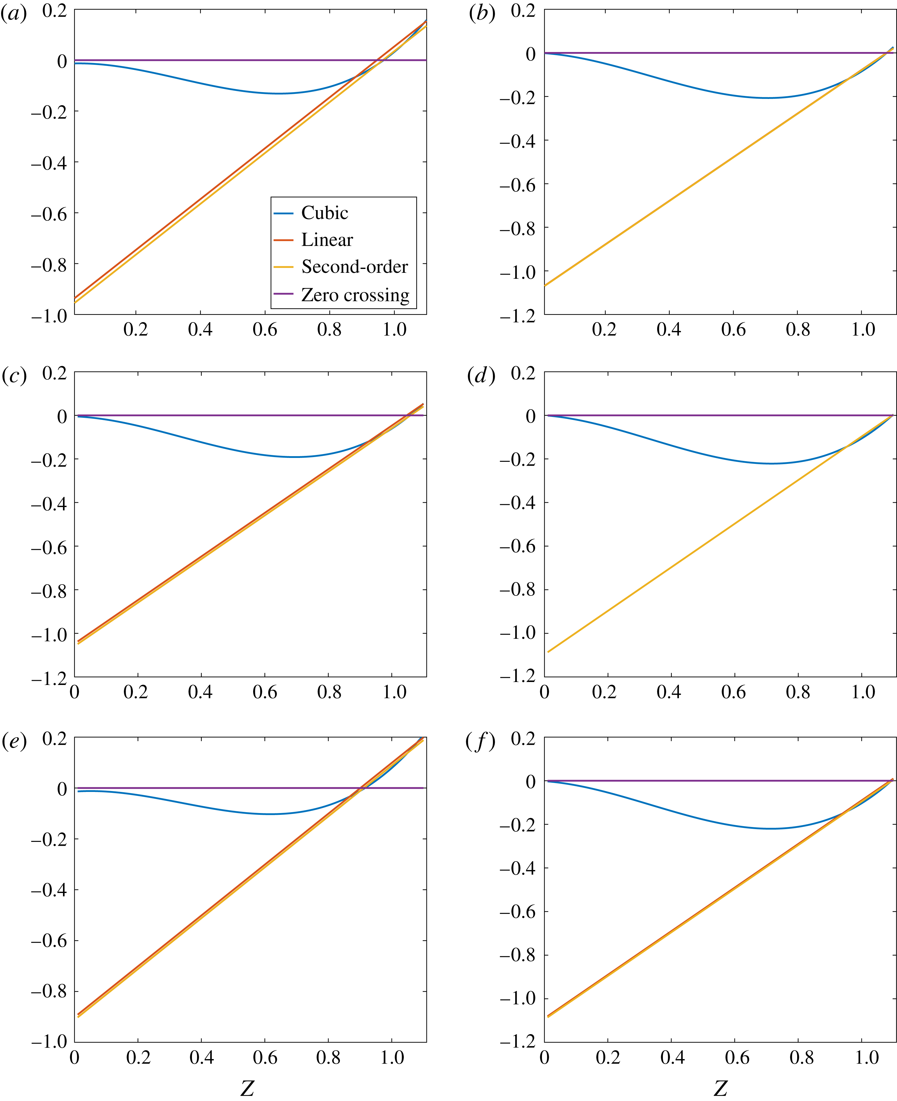
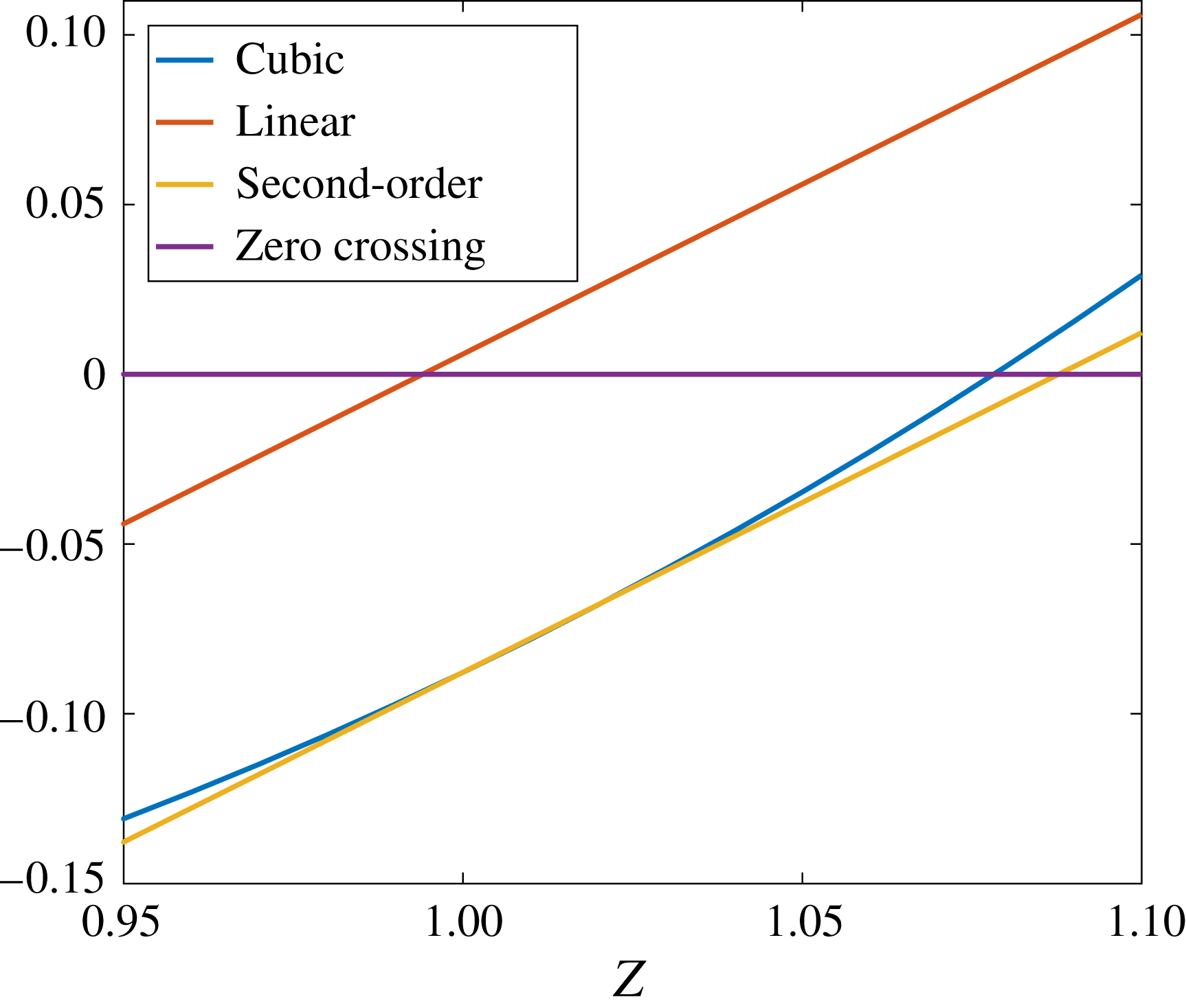
Further analysis and development of the linearization is provided in the appendices. In appendix A, a comparison is made between the exact solution and the linear solution of the cubic EoS. It is shown there that the linear solution can accurately give the solution to the cubic equation which yields the lowest density and therefore is most applicable to compressible flow. The parameter domain where the accuracy is acceptable is identified. It is also shown in appendix A that an iterative approach can yield a higher-order solution which has greater accuracy and yields a much larger domain of validity. The linear treatment is extended to the enthalpy and the speed of sound in appendices B and C, respectively.

3.1 Results for isentropic flow

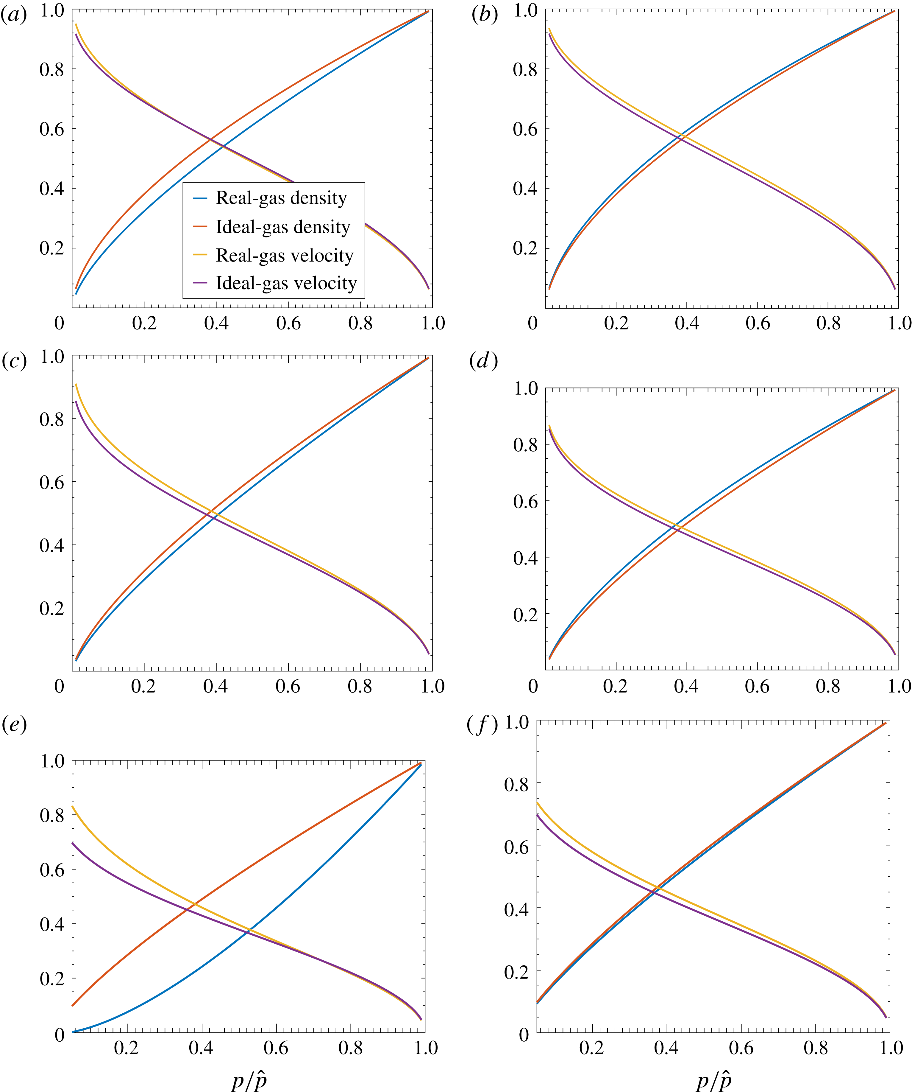
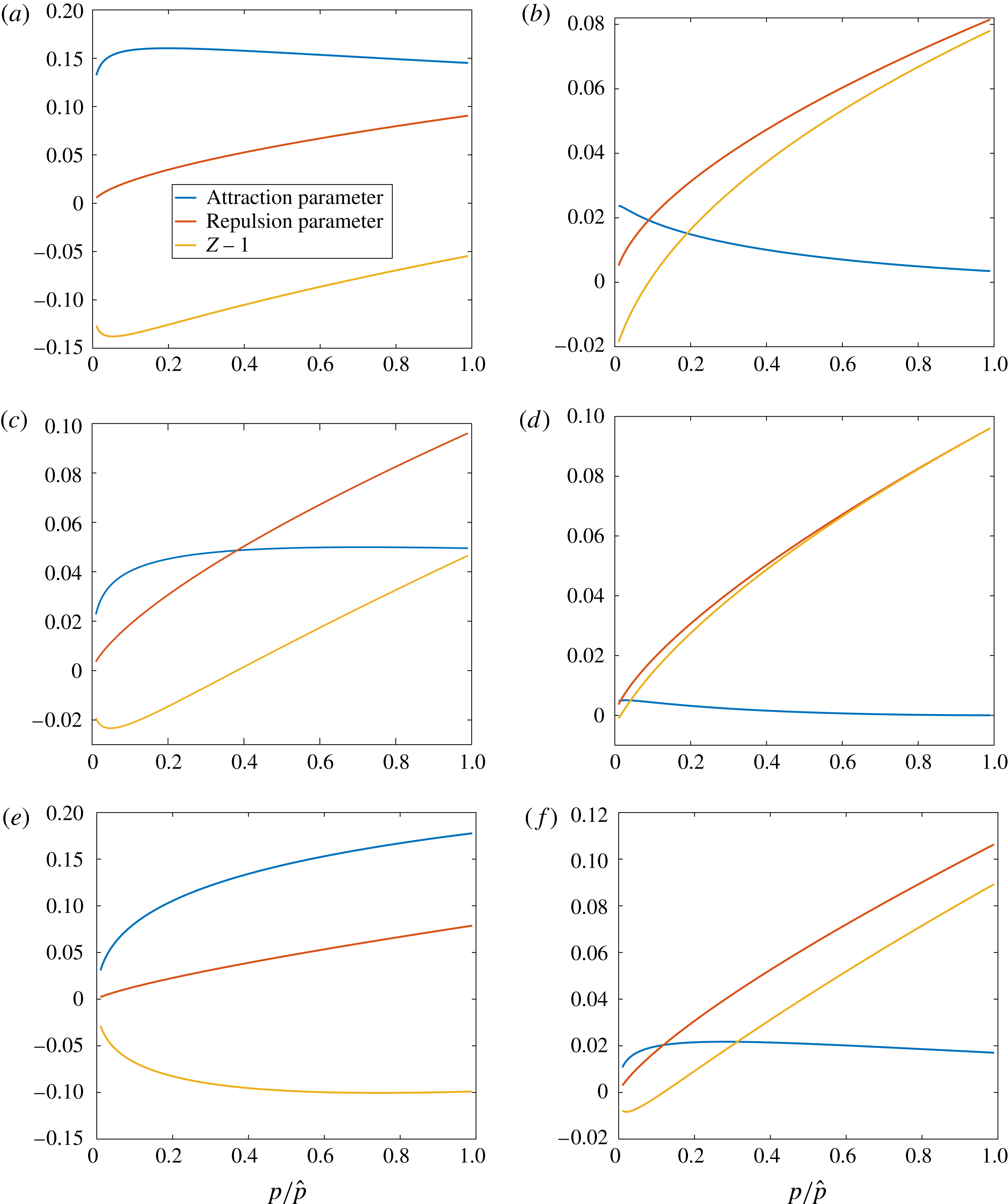
Figure 1 shows argon flow, nitrogen flow and carbon dioxide flow results with non-dimensional values for $\unicode[STIX]{x1D70C}$ and velocity $u$ as functions of the normalized $p$ for six cases, two for each gas. Comparisons are made with ideal-gas results. Although all calculations here involve temperatures and pressures in a range that extends from above to well above standard conditions, including values above the critical values, the cases of figure 1(a,c,e) are identified as ‘lower-temperature’ cases while figure 1(b,d,f) present the ‘higher-temperature’ cases. For the higher-temperature cases, the maximum $Z$ occurs at the highest pressure of 30 MPa. The normalized density is higher for the real gas than for the ideal gas; however, the two stagnation densities used for normalization differ by the factor $\hat{Z}$ , which is the compressibility factor at the stagnation condition. (Pressure, temperature, enthalpy, velocity and sound speed are all normalized by the same values for the real and ideal gases; normalization of density is different.) Thus, the dimensional real-gas density is actually lower than the ideal-gas value. For example, for nitrogen in figure 1(d), the normalized density is a few per cent higher for the real gas. However, $\hat{Z}=1.097$ ; thus, the real-gas dimensional density is approximately 8 % lower than the ideal-gas value in the mid-range of the expansion. For the lower-temperature cases, the value of $\hat{Z}$ can fall below the ideal-gas value. For example, with carbon dioxide in figure 1(e), the real-gas normalized density is a few per cent higher than the ideal-gas normalized density. 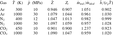However, here $\hat{Z}=0.901$ as shown in table 2. Thus, the stagnation density for the real gas is 11 % higher than for the ideal gas and the dimensional real-gas density exceeds the ideal-gas density by approximately 15 % in the mid-pressure range. In this lower temperature range, the attractive molecular forces that influence $A$ are more effective than the repulsive forces that influence $B$ . The effect of the variation of $\hat{Z}$ from the ideal-gas value is most significant here on density. At high pressures, the intermolecular forces prevent the increase of density in proportion to the pressure as would occur with the ideal gas. In the next section, the consequence for mass flow through a choked nozzle is shown.

Figure 1.

Solutions for non-dimensional density and velocity versus non-dimensional pressure: (a) argon, 300 K, 10 MPa; (b) argon, 1000 K, 30 MPa; (c) nitrogen, 400 K, 12 MPa; (d) nitrogen, 1000 K, 30 MPa; (e) carbon dioxide, 450 K, 10 MPa; (f) carbon dioxide, 1000 K, 30 MPa.

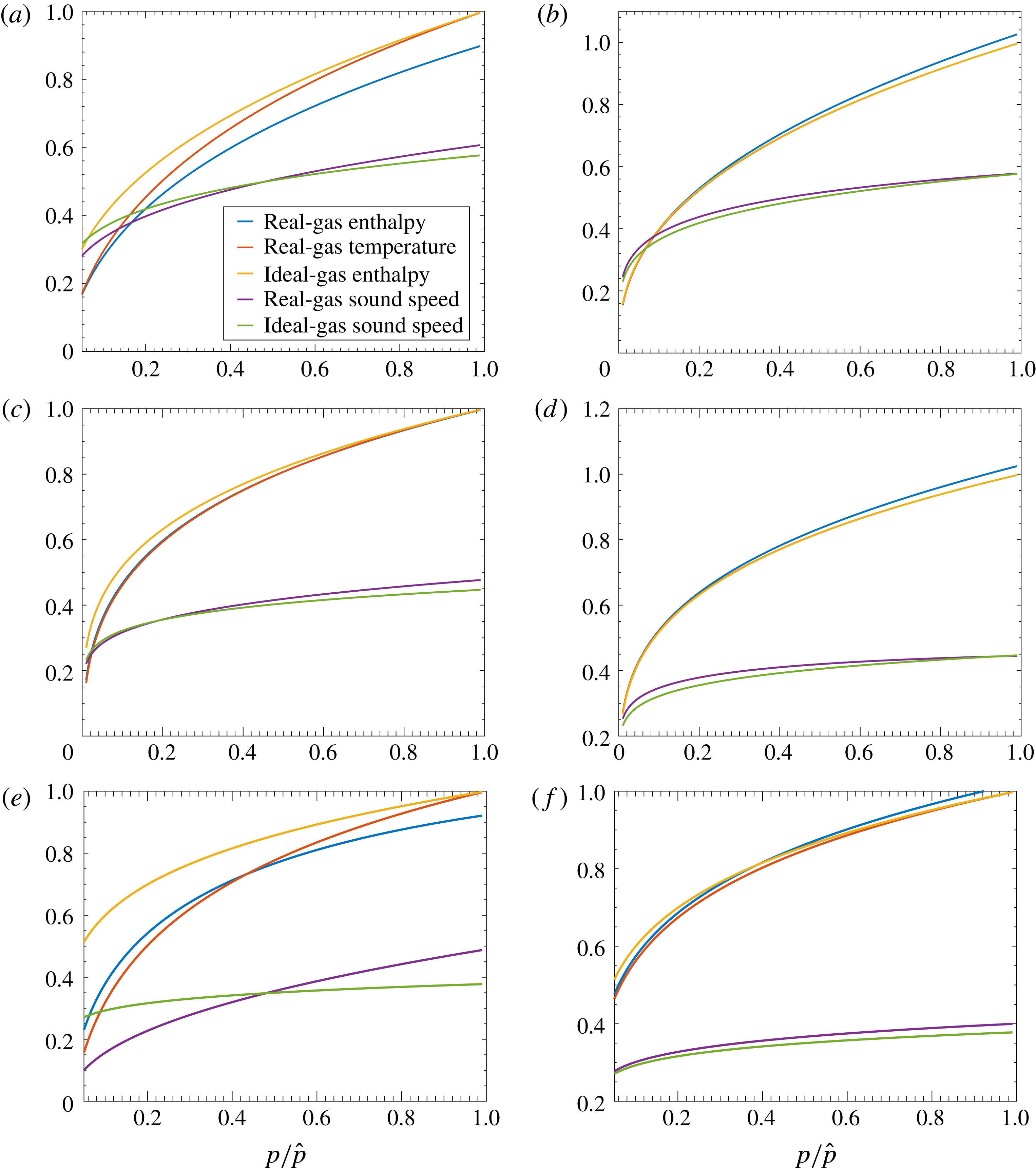
The real-gas velocity generally exceeds the ideal-gas value for both the higher and lower stagnation temperature cases. Accordingly, figure 2 shows that the real-gas enthalpy decreases faster than the ideal-gas enthalpy with decreasing pressure. The stagnation enthalpy for the same stagnation temperature differs between the real and ideal gases.

As table 2 indicates, the cases at higher stagnation temperature generally have real-gas enthalpy exceeding the ideal-gas enthalpy, while the cases at lower stagnation temperature sometimes have real-gas enthalpy values below the ideal-gas enthalpy values. The kinetic energy that can manifest from an expansion increases with increasing stagnation enthalpy.

Table 2.

Comparison between ideal-gas flow and real-gas flow: compressibility factors and ratios for stagnation enthalpy and mass flux.

Enthalpy and temperature for isentropic flows of argon, nitrogen and carbon dioxide are presented in figure 2 as functions of the non-dimensional pressure for both the real and ideal gases. Generally, the normalized real-gas enthalpy differs from the normalized temperature for the real gas by a few per cent for those conditions. The normalized temperatures differ less significantly for the real gas and ideal gas. By construction, normalized temperature equals normalized enthalpy for the ideal gas. At higher stagnation temperatures, the real-gas enthalpy is higher than either the real-gas temperature or the ideal-gas enthalpy (temperature) for the three gases, as seen in figure 2(b,d,f). This implies that there is more energy in the real gas at those same conditions and explains the larger velocity obtained for the real gas in an isentropic expansion. However, a reversal might occur at lower stagnation temperatures, as seen in figure 2(a,c); the ideal-gas enthalpy and temperature values can exceed those for the real gas.

Figure 2.

Solutions for non-dimensional enthalpy, temperature and sound speed versus non-dimensional pressure: (a) argon, 300 K, 10 MPa; (b) argon, 1000 K, 30 MPa; (c) nitrogen, 400 K, 12 MPa; (d) nitrogen, 1000 K, 30 MPa; (e) carbon dioxide, 450 K, 10 MPa; (f) carbon dioxide, 1000 K, 30 MPa.

At higher stagnation temperature, the real gas has a higher sound speed than the ideal gas at the same temperature and pressure. At lower stagnation temperatures, the relative magnitudes can be reversed.

4.1 Values at the sonic location

At the sonic point, where $u=c$ and $u^{2}=c^{2}$ , use of (D 13) and (D 17) yields a condition for the pressure value there. Using subscript $t$ for that point and using coefficient definitions from (D 5), it can be stated that

(4.5) $$\begin{eqnarray}\displaystyle \frac{\unicode[STIX]{x1D6FE}+1}{2}\left(\frac{p_{t}}{\hat{p}}\right)^{(\unicode[STIX]{x1D6FE}-1)/\unicode[STIX]{x1D6FE}} & = & \displaystyle 1+(\unicode[STIX]{x1D706}_{1}-\unicode[STIX]{x1D706}_{b})\left[\frac{\unicode[STIX]{x1D6FE}-1}{\unicode[STIX]{x1D6FE}}\frac{p_{t}}{\hat{p}}-\left(\frac{p_{t}}{\hat{p}}\right)^{(\unicode[STIX]{x1D6FE}-1)/\unicode[STIX]{x1D6FE}}+\frac{1}{\unicode[STIX]{x1D6FE}}\right]\nonumber\\ \displaystyle & & \displaystyle -\,\unicode[STIX]{x1D706}_{2}\left[(\unicode[STIX]{x1D6FE}-1)\left(\frac{p_{t}}{\hat{p}}\right)^{1/\unicode[STIX]{x1D6FE}}-\left(\frac{p_{t}}{\hat{p}}\right)^{(\unicode[STIX]{x1D6FE}-1)/\unicode[STIX]{x1D6FE}}+2-\unicode[STIX]{x1D6FE}\right]\nonumber\\ \displaystyle & & \displaystyle +\,\unicode[STIX]{x1D706}_{3}\left[\frac{2(\unicode[STIX]{x1D6FE}-1)}{\unicode[STIX]{x1D6FE}+1}\left(\frac{p_{t}}{\hat{p}}\right)^{(1-\unicode[STIX]{x1D6FE})/2\unicode[STIX]{x1D6FE}}-\left(\frac{p_{t}}{\hat{p}}\right)^{(\unicode[STIX]{x1D6FE}+1)/\unicode[STIX]{x1D6FE}}+\frac{3-\unicode[STIX]{x1D6FE}}{\unicode[STIX]{x1D6FE}+1}\right]\nonumber\\ \displaystyle & & \displaystyle +\,\frac{\unicode[STIX]{x1D6FE}-1}{2}\left(\frac{p_{t}}{\hat{p}}\right)^{(\unicode[STIX]{x1D6FE}-1)/\unicode[STIX]{x1D6FE}}\left[\unicode[STIX]{x1D706}_{b}-\unicode[STIX]{x1D706}_{1}+\unicode[STIX]{x1D706}_{2}-\unicode[STIX]{x1D706}_{3}-2(\unicode[STIX]{x1D706}_{b}-\unicode[STIX]{x1D706}_{1})\left(\frac{p_{t}}{\hat{p}}\right)^{1/\unicode[STIX]{x1D6FE}}\right.\nonumber\\ \displaystyle & & \displaystyle -\left.\frac{2\unicode[STIX]{x1D706}_{2}}{\unicode[STIX]{x1D6FE}}\left(\frac{p_{t}}{\hat{p}}\right)^{(2-\unicode[STIX]{x1D6FE})/\unicode[STIX]{x1D6FE}}+\frac{(5-\unicode[STIX]{x1D6FE})\unicode[STIX]{x1D706}_{3}}{2}\left(\frac{p_{t}}{\hat{p}}\right)^{(3-\unicode[STIX]{x1D6FE})/2\unicode[STIX]{x1D6FE}}\right]\nonumber\\ \displaystyle & = & \displaystyle 1+(\unicode[STIX]{x1D706}_{b}-\unicode[STIX]{x1D706}_{1})\left[\frac{\unicode[STIX]{x1D6FE}+1}{2}\left(\frac{p_{t}}{\hat{p}}\right)^{(\unicode[STIX]{x1D6FE}-1)/\unicode[STIX]{x1D6FE}}-\frac{\unicode[STIX]{x1D6FE}^{2}-1}{\unicode[STIX]{x1D6FE}}\frac{p_{t}}{\hat{p}}-\frac{1}{\unicode[STIX]{x1D6FE}}\right]\nonumber\\ \displaystyle & & \displaystyle +\,\unicode[STIX]{x1D706}_{2}\left[\frac{\unicode[STIX]{x1D6FE}+1}{2}\left(\frac{p_{t}}{\hat{p}}\right)^{(\unicode[STIX]{x1D6FE}-1)/\unicode[STIX]{x1D6FE}}-\frac{\unicode[STIX]{x1D6FE}^{2}-1}{\unicode[STIX]{x1D6FE}}\left(\frac{p_{t}}{\hat{p}}\right)^{1/\unicode[STIX]{x1D6FE}}+\unicode[STIX]{x1D6FE}-2\right]\nonumber\\ \displaystyle & & \displaystyle +\,\unicode[STIX]{x1D706}_{3}\left[\frac{\unicode[STIX]{x1D6FE}-1}{2}\left(\frac{p_{t}}{\hat{p}}\right)^{(\unicode[STIX]{x1D6FE}-1)/\unicode[STIX]{x1D6FE}}+\frac{2(\unicode[STIX]{x1D6FE}-1)}{\unicode[STIX]{x1D6FE}+1}\left(\frac{p_{t}}{\hat{p}}\right)^{(1-\unicode[STIX]{x1D6FE})/2\unicode[STIX]{x1D6FE}}\right.\nonumber\\ \displaystyle & & \displaystyle -\left.\left(\frac{3-\unicode[STIX]{x1D6FE}}{2}\right)^{2}\left(\frac{p_{t}}{\hat{p}}\right)^{(\unicode[STIX]{x1D6FE}+1)/\unicode[STIX]{x1D6FE}}+\frac{3-\unicode[STIX]{x1D6FE}}{\unicode[STIX]{x1D6FE}+1}\right].\end{eqnarray}$$

To zeroth order, $p_{t}/\hat{p}=[2/(\unicode[STIX]{x1D6FE}+1)]^{\unicode[STIX]{x1D6FE}/(\unicode[STIX]{x1D6FE}-1)}$ , which may be substituted into the first-order terms. Define

(4.6a-c ) $$\begin{eqnarray}\displaystyle \unicode[STIX]{x1D6E4}_{0}\equiv \frac{2}{\unicode[STIX]{x1D6FE}+1},\quad \unicode[STIX]{x1D6E4}_{1}\equiv \left(\frac{2}{\unicode[STIX]{x1D6FE}+1}\right)^{\unicode[STIX]{x1D6FE}/(\unicode[STIX]{x1D6FE}-1)},\quad \unicode[STIX]{x1D6E4}_{2}\equiv \left(\frac{2}{\unicode[STIX]{x1D6FE}+1}\right)^{1/(\unicode[STIX]{x1D6FE}-1)}. & & \displaystyle\end{eqnarray}$$

Then, it is obtained that

(4.7) $$\begin{eqnarray}\displaystyle \frac{p_{t}}{\hat{p}} & = & \displaystyle \unicode[STIX]{x1D6E4}_{1}\left\{\vphantom{\left(\frac{2}{\unicode[STIX]{x1D6FE}+1}\right)^{1/2}}1+(\unicode[STIX]{x1D706}_{b}-\unicode[STIX]{x1D706}_{1})\left[\frac{\unicode[STIX]{x1D6FE}-1}{\unicode[STIX]{x1D6FE}}-\frac{(\unicode[STIX]{x1D6FE}^{2}-1)}{\unicode[STIX]{x1D6FE}}\unicode[STIX]{x1D6E4}_{1}\right]+\unicode[STIX]{x1D706}_{2}\left[\unicode[STIX]{x1D6FE}-1-\frac{\unicode[STIX]{x1D6FE}^{2}-1}{\unicode[STIX]{x1D6FE}}\unicode[STIX]{x1D6E4}_{2}\right]\right.\nonumber\\ \displaystyle & & \displaystyle \left.+\,\unicode[STIX]{x1D706}_{3}\left[\left(\frac{2}{\unicode[STIX]{x1D6FE}+1}\right)^{1/2}(\unicode[STIX]{x1D6FE}-1)-\left(\frac{3-\unicode[STIX]{x1D6FE}}{2}\right)^{2}\unicode[STIX]{x1D6E4}_{1}\unicode[STIX]{x1D6E4}_{2}+\unicode[STIX]{x1D6E4}_{0}\right]\right\}^{\unicode[STIX]{x1D6FE}/(\unicode[STIX]{x1D6FE}-1)}.\end{eqnarray}$$

Now, substitution from (4.7) into (D 7), (D 10), (D 14), (D 17) and (D 12) allows determination of other variables at the sonic point as functions of $\unicode[STIX]{x1D6FE}$ , $\hat{A}$ and $\hat{B}$ . The values of $\unicode[STIX]{x1D70C}_{t}$ and $c_{t}$ are especially useful in determining mass flow and thrust for a choked-nozzle configuration. For example,

(4.8) $$\begin{eqnarray}\displaystyle \frac{\unicode[STIX]{x1D70C}_{t}}{\hat{\unicode[STIX]{x1D70C}}}=\left(\frac{p_{t}}{\hat{p}}\right)^{1/\unicode[STIX]{x1D6FE}}+(\unicode[STIX]{x1D706}_{1}-\unicode[STIX]{x1D706}_{b})[\unicode[STIX]{x1D6E4}_{2}^{2}-\unicode[STIX]{x1D6E4}_{2}]+\unicode[STIX]{x1D706}_{2}\left[\unicode[STIX]{x1D6E4}_{2}-\frac{\unicode[STIX]{x1D6E4}_{2}^{2}}{\unicode[STIX]{x1D6E4}_{0}}\right]+\unicode[STIX]{x1D706}_{3}[\unicode[STIX]{x1D6E4}_{2}^{5/2}\unicode[STIX]{x1D6E4}_{1}^{-1/2}-\unicode[STIX]{x1D6E4}_{2}] & & \displaystyle\end{eqnarray}$$

and

(4.9) $$\begin{eqnarray}\displaystyle \frac{c_{t}}{(2c_{p}\hat{T})^{1/2}} & = & \displaystyle \left(\frac{\unicode[STIX]{x1D6FE}-1}{2}\right)^{1/2}\hat{Z}^{1/2}\left(\frac{p_{t}}{\hat{p}}\right)^{(\unicode[STIX]{x1D6FE}-1)/2\unicode[STIX]{x1D6FE}}\left[\vphantom{\frac{\unicode[STIX]{x1D6E4}_{2}}{\unicode[STIX]{x1D6E4}_{0}^{1/2}}}1-\unicode[STIX]{x1D706}_{b}+\unicode[STIX]{x1D706}_{1}-\unicode[STIX]{x1D706}_{2}+\unicode[STIX]{x1D706}_{3}\right.\nonumber\\ \displaystyle & & \displaystyle +\left.2(\unicode[STIX]{x1D706}_{b}-\unicode[STIX]{x1D706}_{1})\unicode[STIX]{x1D6E4}_{2}+\frac{2\unicode[STIX]{x1D706}_{2}}{\unicode[STIX]{x1D6FE}}\frac{\unicode[STIX]{x1D6E4}_{2}^{2}}{\unicode[STIX]{x1D6E4}_{1}}-\frac{(5-\unicode[STIX]{x1D6FE})\unicode[STIX]{x1D706}_{3}}{2}\frac{\unicode[STIX]{x1D6E4}_{2}}{\unicode[STIX]{x1D6E4}_{0}^{1/2}}\right]^{1/2},\end{eqnarray}$$

where the lower-order solution for $p_{t}$ has been substituted into the higher-order terms of (4.8) and (4.9).

4.2 Dependence on Mach number

From (D 13) and (D 17), the Mach number $M$ can be determined as a function of pressure in the one-dimensional isentropic flow, namely

(4.10) $$\begin{eqnarray}\displaystyle M=\frac{u}{c}=\left[\left(\frac{2}{\unicode[STIX]{x1D6FE}-1}\right)\left(\frac{p}{\hat{p}}\right)^{(1-\unicode[STIX]{x1D6FE})/\unicode[STIX]{x1D6FE}}~\frac{\displaystyle 1-\left(\frac{p}{\hat{p}}\right)^{(\unicode[STIX]{x1D6FE}-1)/\unicode[STIX]{x1D6FE}}+\unicode[STIX]{x1D6EC}_{2}\left(\frac{p}{\hat{p}}\right)}{\displaystyle 1+\unicode[STIX]{x1D6EC}_{3}\left(\frac{p}{\hat{p}}\right)}\right]^{1/2}, & & \displaystyle\end{eqnarray}$$

where the functions $\unicode[STIX]{x1D6EC}_{2}$ and $\unicode[STIX]{x1D6EC}_{3}$ are defined by (D 11) and (D 16) and encapsulate the first-order corrections for the real gas.

To lowest order, one obtains is the ideal-gas result $p/\hat{p}=m^{\unicode[STIX]{x1D6FE}/(1-\unicode[STIX]{x1D6FE})}$ where $m\equiv 1+[(\unicode[STIX]{x1D6FE}-1)/2]M^{2}$ . This may be substituted into the higher-order terms in (4.10) to obtain the approximation for pressure as a function of Mach number:

(4.11) $$\begin{eqnarray}\displaystyle \frac{p}{\hat{p}}=\left[1+\frac{\unicode[STIX]{x1D6FE}-1}{2}M^{2}[1+\unicode[STIX]{x1D6EC}_{2}(m^{\unicode[STIX]{x1D6FE}/(1-\unicode[STIX]{x1D6FE})})]-\unicode[STIX]{x1D6EC}_{1}(m^{\unicode[STIX]{x1D6FE}/(1-\unicode[STIX]{x1D6FE})})\right]^{\unicode[STIX]{x1D6FE}/(1-\unicode[STIX]{x1D6FE})}, & & \displaystyle\end{eqnarray}$$

where $\unicode[STIX]{x1D6EC}_{1}$ is defined by (D 8).

4.3 Dependence on cross-sectional area

From the one-dimensional continuity relation for choked flow through a nozzle, it follows that

(4.12) $$\begin{eqnarray}\displaystyle \frac{A}{A_{t}}=\frac{\unicode[STIX]{x1D70C}_{t}/(\hat{Z}\hat{\unicode[STIX]{x1D70C}})}{\unicode[STIX]{x1D70C}/\hat{\unicode[STIX]{x1D70C}}}\;\frac{\displaystyle c_{t}\left/\sqrt{2c_{p}\hat{T}}\right.}{u\left/\sqrt{2c_{p}\hat{T}}\right.}. & & \displaystyle\end{eqnarray}$$

Substitution from (D 7), (D 14), (D 18) and (4.7) into (4.12) yields $A/A_{t}$ as a function of $p/\hat{p},~\unicode[STIX]{x1D6FE},~\hat{A}$ and $\hat{B}$ . To lowest order, a relation for the ideal-gas flow is given by

(4.13) $$\begin{eqnarray}\displaystyle \frac{A}{A_{t}} & = & \displaystyle \left[1+\frac{\unicode[STIX]{x1D6FE}-1}{2}M^{2}\right]^{1/(\unicode[STIX]{x1D6FE}-1)}\left(\frac{\unicode[STIX]{x1D6FE}-1}{2}M^{2}\right)^{-1/2}\left[1+\frac{\unicode[STIX]{x1D6FE}-1}{2}M^{2}\right]^{1/2}\unicode[STIX]{x1D6E4}_{1}^{1/\unicode[STIX]{x1D6FE}}\left(\frac{\unicode[STIX]{x1D6FE}-1}{\unicode[STIX]{x1D6FE}+1}\right)^{1/2}\nonumber\\ \displaystyle & = & \displaystyle \frac{1}{M}\left[\frac{2}{\unicode[STIX]{x1D6FE}+1}\left(1+\frac{\unicode[STIX]{x1D6FE}-1}{2}M^{2}\right)\right]^{(\unicode[STIX]{x1D6FE}+1)/(2(\unicode[STIX]{x1D6FE}-1))}.\end{eqnarray}$$

To solve (4.12) for $M$ as a function of $A/A_{t}$ , it is convenient to solve prior equation (4.13) for a first-order approximation of $M$ as a function of $A/A_{t}$ . It yields two solutions: one is supersonic and the other is subsonic. Then, the solution for $M$ from this lower-order analysis can be substituted into the first-order terms of (4.12).

4.4 Mass flux and thrust

The mass flux through the choked nozzle ${\dot{m}}$ depends on stagnation pressure, stagnation temperature, ratio of specific heats and throat cross-sectional area:

(4.14) $$\begin{eqnarray}\displaystyle \frac{{\dot{m}}}{\hat{p}A_{t}/(R\hat{T})^{1/2}}=\frac{\unicode[STIX]{x1D70C}_{t}c_{t}A_{t}}{\hat{p}A_{t}/(R\hat{T})^{1/2}}, & & \displaystyle\end{eqnarray}$$

where the inputs from (4.7), (4.8) and (4.9) are made. For the ideal gas, this reduces to

(4.15) $$\begin{eqnarray}\displaystyle {\dot{m}}_{ideal}=\unicode[STIX]{x1D6FE}^{1/2}\left(\frac{2}{\unicode[STIX]{x1D6FE}+1}\right)^{(\unicode[STIX]{x1D6FE}+1)/(2(\unicode[STIX]{x1D6FE}-1))}\frac{\hat{p}A_{t}}{(R\hat{T})^{1/2}}. & & \displaystyle\end{eqnarray}$$

The product $\unicode[STIX]{x1D70C}_{t}u_{t}=\unicode[STIX]{x1D70C}_{t}c_{t}$ in (4.14) can be determined in several ways: (i) equations (4.8) and (4.9) can be used; (ii) the values of $\unicode[STIX]{x1D70C}$ and $u$ can be used at the pressure where $u=c$ ; or (iii) the magnitude of the maximum value of the product $\unicode[STIX]{x1D70C}u$ can be determined over the pressure range. The numerical results are close but differences occur because of second-order errors in the linear method. The third approach has arbitrarily been selected.

The thrust force $F$ can also be determined as a function of stagnation properties, values of the variables at the nozzle throat and exit, and cross-sectional area. If the subscripts $e$ and $a$ , respectively, denote exit values and ambient values, the standard relation is $F={\dot{m}}u_{e}+(p_{e}-p_{a})A_{e}$ . Thus, the non-dimensional thrust is given as

(4.16) $$\begin{eqnarray}\displaystyle \frac{F}{\hat{p}A_{t}}=\frac{\unicode[STIX]{x1D70C}_{t}c_{t}u_{e}}{\hat{p}}+\left(\frac{p}{\hat{p}}-\frac{p_{a}}{\hat{p}}\right)\frac{A_{e}}{A_{t}}. & & \displaystyle\end{eqnarray}$$

The specific impulse is defined as $I\equiv F/({\dot{m}}g)$ with units of seconds. A normalized value can be calculated from (4.14) and (4.16):

(4.17) $$\begin{eqnarray}\displaystyle \frac{Ig}{\sqrt{R\hat{T}}}=\frac{F/(\hat{p}A_{t})}{{\dot{m}}(R\hat{T})^{1/2}/(\hat{p}A_{t})}. & & \displaystyle\end{eqnarray}$$

4.5 Results for one-dimensional flow

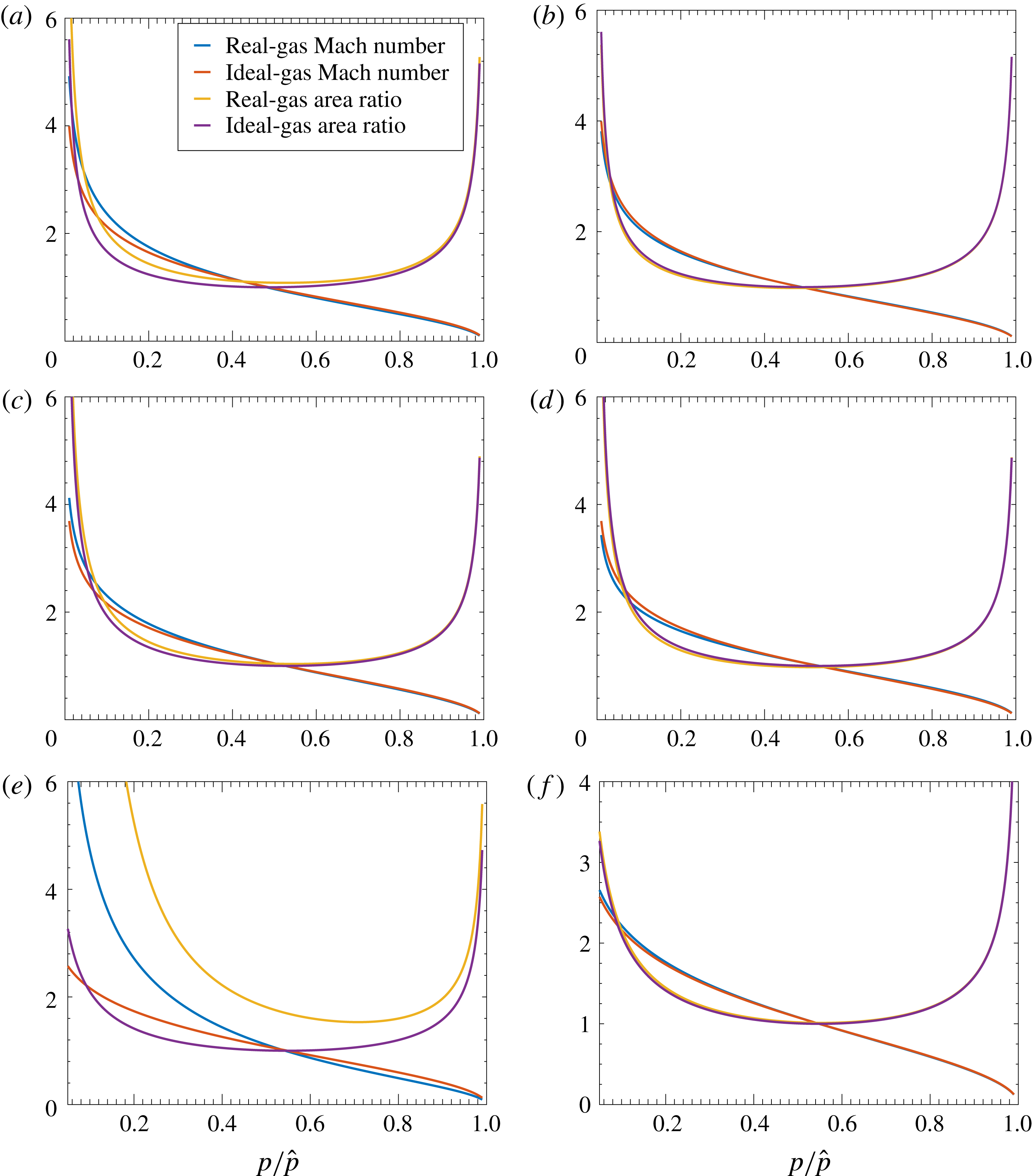
Figure 3 shows comparisons of Mach number and normalized cross-sectional area versus normalized pressure for both real and ideal flows. Mach number is generally slightly higher for real gases at the lower stagnation temperatures; at higher temperatures, no general behaviour appears. This comparison is at a given pressure not a given cross-sectional area. This point is noteworthy because the areas for the real gas and ideal gas at that pressure can differ. Generally, in the supersonic region at lower stagnation temperatures, for identical Mach number, the real gas has a higher pressure. At a given pressure and lower stagnation temperatures, the real gas has larger cross-sectional area in the supersonic domain.

Figure 3.

Solutions for Mach number and area ratio versus non-dimensional pressure for choked-nozzle flow: (a) argon, 300 K, 10 MPa; (b) argon, 1000 K, 30 MPa; (c) nitrogen, 400 K, 12 MPa; (d) nitrogen, 1000 K, 30 MPa; (e) carbon dioxide, 450 K, 10 MPa; (f) carbon dioxide, 1000 K, 30 MPa.

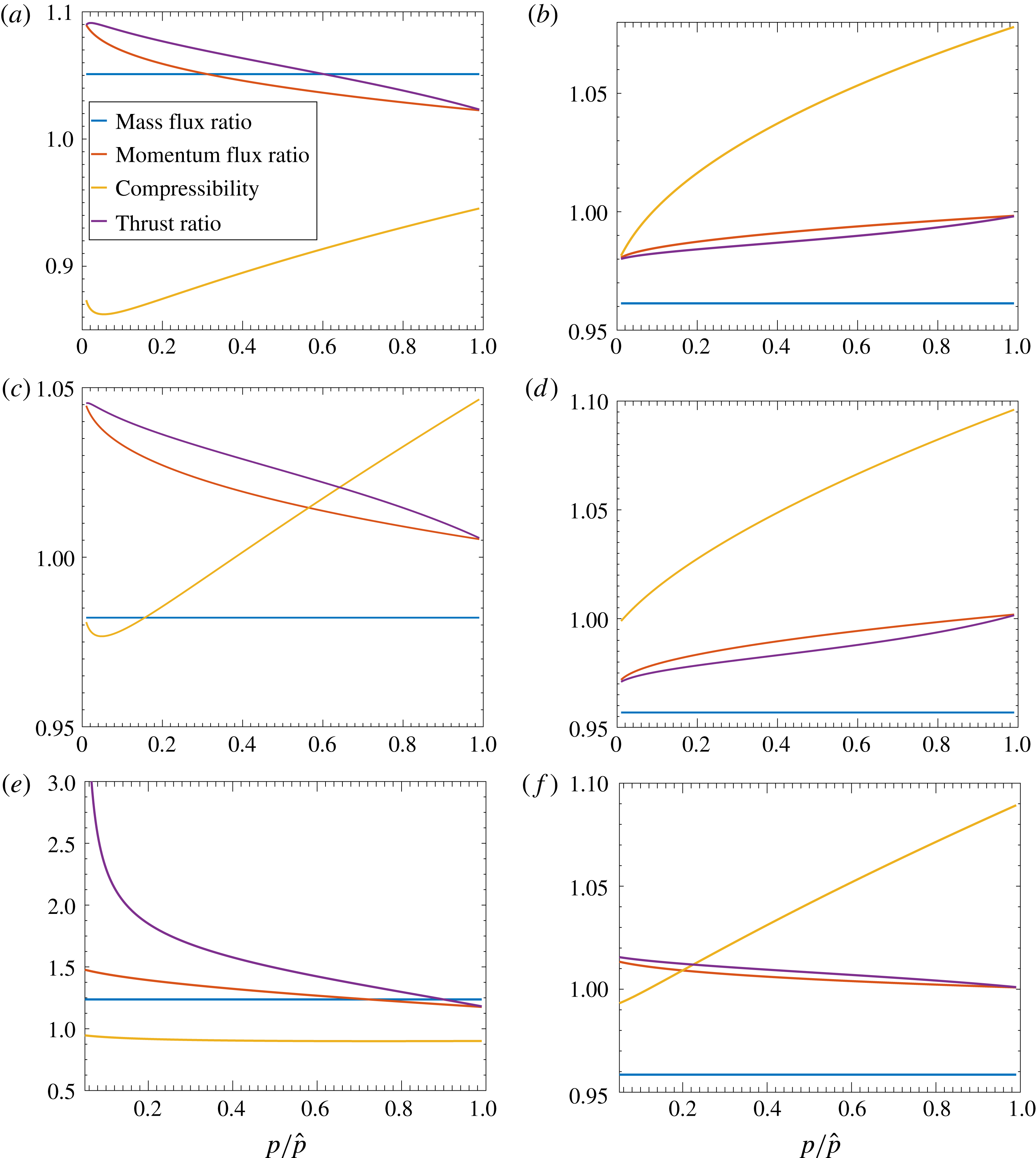
Figure 4 gives comparisons between the real gas and ideal gas for mass flux ${\dot{m}}/{\dot{m}}_{ideal}$ , momentum flux ${\dot{m}}u/({\dot{m}}_{ideal}u_{ideal})$ , thrust, compressibility factor $Z$ and thrust ratio $F/F_{ideal}$ . Real-gas mass flux is generally lower (higher) than ideal-gas flux for flows where $Z-1$ is positive (negative). This rule generally occurs at higher stagnation temperatures, with some deviation at lower stagnation temperatures. Figure 4(c) shows a transitional case for the value of $Z-1$ . This higher-temperature reduction in allowable mass flux is highly relevant to combustion at high pressures. The compressibility factor generally increases with increasing pressure and increasing stagnation temperature. Previous works (Johnson Reference Johnson1964; Ascough Reference Ascough1968; Kim et al. Reference Kim, Kim, Setoguchi and Matsuo2008) reported mass flux through choked nozzles for generally low stagnation pressures. With the exception of a case with water vapour (i.e. steam) flow (Johnson Reference Johnson1964), they found the real-gas flow had a greater mass flux than the ideal-gas flow. It follows that real-gas flow gives less mass discharge at higher stagnation temperatures and the reversal is related to the change in relative magnitudes of the repulsion and attraction parameters.

Figure 4.

Comparison of real-gas to ideal-gas ratios of mass flux, momentum flux and thrust between real-gas nozzle flow and ideal-gas nozzle flow: (a) argon, 300 K, 10 MPa; (b) argon, 1000 K, 30 MPa; (c) nitrogen, 400 K, 12 MPa; (d) nitrogen, 1000 K, 30 MPa; (e) carbon dioxide, 450 K, 10 MPa; (f) carbon dioxide, 1000 K, 30 MPa.

The momentum flux ratio and the thrust ratio exhibit similar trends, always decreasing at lower stagnation temperatures with increasing pressure. At optimal thrust, momentum flux and thrust become equal. For the very high stagnation pressures considered, the expansions have not reached a cross-sectional area that gives the designated ambient pressure (1 bar). Thus, the momentum flux ratio exceeds the thrust ratio.

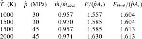
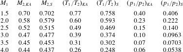
It is interesting to examine the optimal thrust that manifests when the supersonic flow is expanded to ambient pressure. Several combinations of stagnation pressure and temperature were taken, with results shown in table 3 for nitrogen with an expansion to 1 bar. In all cases, the mass flux for the real gas was a few per cent below the ideal-gas values. Generally, the real-gas thrust is lower than the ideal-gas thrust at higher stagnation pressures and temperatures.

Table 3.

Optimal thrust values for nitrogen flow through a nozzle.

There is longstanding knowledge that, at high pressures, the allowable mass flux through a choked nozzle can differ by a few per cent between the ideal gas and a real gas. Here, one finds for nitrogen in figure 4(c) that, at 400 K $(720^{\circ }\text{R})$ and 120 bar, $Z=104.7$ and mass flux defect (i.e. one minus mass flux ratio) is 0.017. Considering differences in the EoS, these values compare favourably with the values of 103.7 and 0.027 reported by Johnson (Reference Johnson1964) for $700^{\circ }\text{R}$ and 100 atm.

5.1 Riemann invariant construction

Define $\unicode[STIX]{x1D716}\equiv \unicode[STIX]{x1D6EC}_{1}-\unicode[STIX]{x1D6EC}_{3}/(\unicode[STIX]{x1D6FE}-1)$ and substitute into (5.1) for $\unicode[STIX]{x1D70C}^{\prime }$ :

(5.6) $$\begin{eqnarray}\displaystyle & \displaystyle \frac{2}{\unicode[STIX]{x1D6FE}-1}\left[\frac{\unicode[STIX]{x2202}c^{\prime }}{\unicode[STIX]{x2202}t^{\prime }}+u^{\prime }\frac{\unicode[STIX]{x2202}c^{\prime }}{\unicode[STIX]{x2202}x^{\prime }}\right]+c^{\prime }\frac{\unicode[STIX]{x2202}\unicode[STIX]{x1D716}}{\unicode[STIX]{x2202}t^{\prime }}+u^{\prime }c^{\prime }\frac{\unicode[STIX]{x2202}\unicode[STIX]{x1D716}}{\unicode[STIX]{x2202}x^{\prime }}+c^{\prime }\frac{\unicode[STIX]{x2202}u^{\prime }}{\unicode[STIX]{x2202}x^{\prime }}=0, & \displaystyle\end{eqnarray}$$

(5.7) $$\begin{eqnarray}\displaystyle & \displaystyle \frac{\unicode[STIX]{x2202}u^{\prime }}{\unicode[STIX]{x2202}t^{\prime }}+u^{\prime }\frac{\unicode[STIX]{x2202}u^{\prime }}{\unicode[STIX]{x2202}x^{\prime }}+c^{\prime }\frac{2}{\unicode[STIX]{x1D6FE}-1}\frac{\unicode[STIX]{x2202}c^{\prime }}{\unicode[STIX]{x2202}x^{\prime }}+c^{\prime 2}\frac{\unicode[STIX]{x2202}\unicode[STIX]{x1D716}}{\unicode[STIX]{x2202}x^{\prime }}=0. & \displaystyle\end{eqnarray}$$

Using the lowest-order relation $p^{\prime }=(2c^{\prime 2}/(\unicode[STIX]{x1D6FE}-1))^{\unicode[STIX]{x1D6FE}/(\unicode[STIX]{x1D6FE}-1)}$ , $\unicode[STIX]{x1D716},~\unicode[STIX]{x1D6EC}_{1}$ and $\unicode[STIX]{x1D6EC}_{3}$ can be converted to functions of $c^{\prime }$ . Then, a function $\unicode[STIX]{x1D6F9}(c^{\prime })\equiv \int c^{\prime }\,\text{d}\unicode[STIX]{x1D716}=\int c^{\prime }(\text{d}\unicode[STIX]{x1D716}/\text{d}c^{\prime })\,\text{d}c^{\prime }$ is created. The function $\unicode[STIX]{x1D6F9}$ provides, for an isentropic path, an integrated effect of the variation from the ideal-gas behaviour. This allows reorganization of the continuity and momentum equations by addition and subtraction to yield

(5.8) $$\begin{eqnarray}\displaystyle & \displaystyle \left[\frac{\unicode[STIX]{x2202}}{\unicode[STIX]{x2202}t^{\prime }}+(u^{\prime }+c^{\prime })\frac{\unicode[STIX]{x2202}}{\unicode[STIX]{x2202}x^{\prime }}\right]\left(u^{\prime }+\frac{2}{\unicode[STIX]{x1D6FE}-1}c^{\prime }+\unicode[STIX]{x1D6F9}(c^{\prime })\right)=0, & \displaystyle\end{eqnarray}$$

(5.9) $$\begin{eqnarray}\displaystyle & \displaystyle \left[\frac{\unicode[STIX]{x2202}}{\unicode[STIX]{x2202}t^{\prime }}+(u^{\prime }-c^{\prime })\frac{\unicode[STIX]{x2202}}{\unicode[STIX]{x2202}x^{\prime }}\right]\left(u^{\prime }-\frac{2}{\unicode[STIX]{x1D6FE}-1}c^{\prime }-\unicode[STIX]{x1D6F9}(c^{\prime })\right)=0. & \displaystyle\end{eqnarray}$$

This yields the two modified Riemann invariants,

(5.10) $$\begin{eqnarray}\displaystyle \left.\begin{array}{@{}c@{}}\displaystyle I_{R}\equiv u^{\prime }+\frac{2}{\unicode[STIX]{x1D6FE}-1}c^{\prime }+\unicode[STIX]{x1D6F9}(c^{\prime }),\\ \displaystyle I_{L}\equiv u^{\prime }-\frac{2}{\unicode[STIX]{x1D6FE}-1}c^{\prime }-\unicode[STIX]{x1D6F9}(c^{\prime }),\end{array}\right\} & & \displaystyle\end{eqnarray}$$

which propagate respectively along the characteristic paths

(5.11) $$\begin{eqnarray}\displaystyle \left.\begin{array}{@{}c@{}}\displaystyle \frac{\text{d}x^{\prime }}{\text{d}t^{\prime }}=(u^{\prime }+c^{\prime }),\\ \displaystyle \frac{\text{d}x^{\prime }}{\text{d}t^{\prime }}=(u^{\prime }-c^{\prime }),\end{array}\right\} & & \displaystyle\end{eqnarray}$$

where the following relations are developed from the definitions given by (D 8) and (D 16):

(5.12) $$\begin{eqnarray}\displaystyle \unicode[STIX]{x1D6EC}_{1} & \equiv & \displaystyle (\unicode[STIX]{x1D706}_{1}-\unicode[STIX]{x1D706}_{b})\left[\left(\frac{p}{\hat{p}}\right)^{1/\unicode[STIX]{x1D6FE}}-1\right]-\unicode[STIX]{x1D706}_{2}\left[\left(\frac{p}{\hat{p}}\right)^{(2-\unicode[STIX]{x1D6FE})/\unicode[STIX]{x1D6FE}}-1\right]\nonumber\\ \displaystyle & & \displaystyle +\,\unicode[STIX]{x1D706}_{3}\left[\left(\frac{p}{\hat{p}}\right)^{(3-\unicode[STIX]{x1D6FE})/2\unicode[STIX]{x1D6FE}}-1\right]\nonumber\\ \displaystyle & = & \displaystyle (\unicode[STIX]{x1D706}_{1}-\unicode[STIX]{x1D706}_{b})\left[\left(\frac{2c^{\prime 2}}{\unicode[STIX]{x1D6FE}-1}\right)^{1/(\unicode[STIX]{x1D6FE}-1)}-1\right]-\unicode[STIX]{x1D706}_{2}\left[\left(\frac{2c^{\prime 2}}{\unicode[STIX]{x1D6FE}-1}\right)^{(2-\unicode[STIX]{x1D6FE})/(\unicode[STIX]{x1D6FE}-1)}-1\right]\nonumber\\ \displaystyle & & \displaystyle +\,\unicode[STIX]{x1D706}_{3}\left[\left(\frac{2c^{\prime 2}}{\unicode[STIX]{x1D6FE}-1}\right)^{(3-\unicode[STIX]{x1D6FE})/2(\unicode[STIX]{x1D6FE}-1)}-1\right],\end{eqnarray}$$

(5.13) $$\begin{eqnarray}\displaystyle \unicode[STIX]{x1D6EC}_{3} & \equiv & \displaystyle -\unicode[STIX]{x1D706}_{b}+\unicode[STIX]{x1D706}_{1}-\unicode[STIX]{x1D706}_{2}+\unicode[STIX]{x1D706}_{3}+\frac{(\unicode[STIX]{x1D6FE}+1)(\unicode[STIX]{x1D706}_{b}-\unicode[STIX]{x1D706}_{1})}{\unicode[STIX]{x1D6FE}}\left(\frac{p}{\hat{p}}\right)^{1/\unicode[STIX]{x1D6FE}}\nonumber\\ \displaystyle & & \displaystyle +\,\frac{2\unicode[STIX]{x1D706}_{2}}{\unicode[STIX]{x1D6FE}}\left(\frac{p}{\hat{p}}\right)^{(2-\unicode[STIX]{x1D6FE})/\unicode[STIX]{x1D6FE}}-\frac{(3+\unicode[STIX]{x1D6FE})\unicode[STIX]{x1D706}_{3}}{2\unicode[STIX]{x1D6FE}}\left(\frac{p}{\hat{p}}\right)^{(3-\unicode[STIX]{x1D6FE})/2\unicode[STIX]{x1D6FE}}\nonumber\\ \displaystyle & = & \displaystyle -\unicode[STIX]{x1D706}_{b}+\unicode[STIX]{x1D706}_{1}-\unicode[STIX]{x1D706}_{2}+\unicode[STIX]{x1D706}_{3}+\frac{(\unicode[STIX]{x1D6FE}+1)(\unicode[STIX]{x1D706}_{b}-\unicode[STIX]{x1D706}_{1})}{\unicode[STIX]{x1D6FE}}\left(\frac{2c^{\prime 2}}{\unicode[STIX]{x1D6FE}-1}\right)^{1/(\unicode[STIX]{x1D6FE}-1)}\nonumber\\ \displaystyle & & \displaystyle +\,\frac{2\unicode[STIX]{x1D706}_{2}}{\unicode[STIX]{x1D6FE}}\left(\frac{2c^{\prime 2}}{\unicode[STIX]{x1D6FE}-1}\right)^{(2-\unicode[STIX]{x1D6FE})/(\unicode[STIX]{x1D6FE}-1)}-\frac{(3+\unicode[STIX]{x1D6FE})\unicode[STIX]{x1D706}_{3}}{2\unicode[STIX]{x1D6FE}}\left(\frac{2c^{\prime 2}}{\unicode[STIX]{x1D6FE}-1}\right)^{(3-\unicode[STIX]{x1D6FE})/2(\unicode[STIX]{x1D6FE}-1)},\quad\end{eqnarray}$$

(5.14) $$\begin{eqnarray}\displaystyle \unicode[STIX]{x1D716}\equiv \unicode[STIX]{x1D6EC}_{1}-\frac{\unicode[STIX]{x1D6EC}_{3}}{\unicode[STIX]{x1D6FE}-1} & = & \displaystyle \frac{\unicode[STIX]{x1D6FE}}{\unicode[STIX]{x1D6FE}-1}(\unicode[STIX]{x1D706}_{b}-\unicode[STIX]{x1D706}_{1}+\unicode[STIX]{x1D706}_{2}-\unicode[STIX]{x1D706}_{3})+\frac{(\unicode[STIX]{x1D6FE}^{2}+1)(\unicode[STIX]{x1D706}_{1}-\unicode[STIX]{x1D706}_{b})}{\unicode[STIX]{x1D6FE}(\unicode[STIX]{x1D6FE}-1)}\left(\frac{2c^{\prime 2}}{\unicode[STIX]{x1D6FE}-1}\right)^{1/(\unicode[STIX]{x1D6FE}-1)}\nonumber\\ \displaystyle & & \displaystyle -\,\frac{(\unicode[STIX]{x1D6FE}^{2}-\unicode[STIX]{x1D6FE}+2)\unicode[STIX]{x1D706}_{2}}{\unicode[STIX]{x1D6FE}(\unicode[STIX]{x1D6FE}-1)}\left(\frac{2c^{\prime 2}}{\unicode[STIX]{x1D6FE}-1}\right)^{(2-\unicode[STIX]{x1D6FE})/(\unicode[STIX]{x1D6FE}-1)}\nonumber\\ \displaystyle & & \displaystyle +\,\frac{(2\unicode[STIX]{x1D6FE}^{2}-\unicode[STIX]{x1D6FE}+3)\unicode[STIX]{x1D706}_{3}}{2\unicode[STIX]{x1D6FE}(\unicode[STIX]{x1D6FE}-1)}\left(\frac{2c^{\prime 2}}{\unicode[STIX]{x1D6FE}-1}\right)^{(3-\unicode[STIX]{x1D6FE})/2(\unicode[STIX]{x1D6FE}-1)}.\end{eqnarray}$$

Consequently, one obtains

(5.15) $$\begin{eqnarray}\displaystyle c^{\prime }\frac{\text{d}\unicode[STIX]{x1D716}}{\text{d}c^{\prime }} & = & \displaystyle 2c^{\prime 2}\frac{\text{d}\unicode[STIX]{x1D716}}{\text{d}(c^{\prime 2})}\nonumber\\ \displaystyle & = & \displaystyle 2\frac{(\unicode[STIX]{x1D6FE}^{2}+1)(\unicode[STIX]{x1D706}_{1}-\unicode[STIX]{x1D706}_{b})}{\unicode[STIX]{x1D6FE}(\unicode[STIX]{x1D6FE}-1)^{2}}\left(\frac{2c^{\prime 2}}{\unicode[STIX]{x1D6FE}-1}\right)^{1/(\unicode[STIX]{x1D6FE}-1)}\nonumber\\ \displaystyle & & \displaystyle -\,2\frac{(\unicode[STIX]{x1D6FE}^{2}-\unicode[STIX]{x1D6FE}+2)(2-\unicode[STIX]{x1D6FE})\unicode[STIX]{x1D706}_{2}}{\unicode[STIX]{x1D6FE}(\unicode[STIX]{x1D6FE}-1)^{2}}\left(\frac{2c^{\prime 2}}{\unicode[STIX]{x1D6FE}-1}\right)^{(2-\unicode[STIX]{x1D6FE})/(\unicode[STIX]{x1D6FE}-1)}\nonumber\\ \displaystyle & & \displaystyle +\,\frac{(2\unicode[STIX]{x1D6FE}^{2}-\unicode[STIX]{x1D6FE}+3)(3-\unicode[STIX]{x1D6FE})\unicode[STIX]{x1D706}_{3}}{2\unicode[STIX]{x1D6FE}(\unicode[STIX]{x1D6FE}-1)^{2}}\left(\frac{2c^{\prime 2}}{\unicode[STIX]{x1D6FE}-1}\right)^{(3-\unicode[STIX]{x1D6FE})/2(\unicode[STIX]{x1D6FE}-1)},\end{eqnarray}$$

(5.16) $$\begin{eqnarray}\displaystyle \unicode[STIX]{x1D6F9}(c^{\prime }) & = & \displaystyle \int c\frac{\text{d}\unicode[STIX]{x1D716}}{\text{d}c^{\prime }}\,\text{d}c^{\prime }\nonumber\\ \displaystyle & = & \displaystyle \frac{(\unicode[STIX]{x1D6FE}^{2}+1)(\unicode[STIX]{x1D706}_{1}-\unicode[STIX]{x1D706}_{b})}{\unicode[STIX]{x1D6FE}(\unicode[STIX]{x1D6FE}+1)}\left(\frac{2}{\unicode[STIX]{x1D6FE}-1}\right)^{\unicode[STIX]{x1D6FE}/(\unicode[STIX]{x1D6FE}-1)}c^{\prime (\unicode[STIX]{x1D6FE}+1)/(\unicode[STIX]{x1D6FE}-1)}\nonumber\\ \displaystyle & & \displaystyle -\,\frac{(\unicode[STIX]{x1D6FE}^{2}-\unicode[STIX]{x1D6FE}+2)(2-\unicode[STIX]{x1D6FE})\unicode[STIX]{x1D706}_{2}}{\unicode[STIX]{x1D6FE}(3-\unicode[STIX]{x1D6FE})}\left(\frac{2}{\unicode[STIX]{x1D6FE}-1}\right)^{1/(\unicode[STIX]{x1D6FE}-1)}c^{\prime (3-\unicode[STIX]{x1D6FE})/(\unicode[STIX]{x1D6FE}-1)}\nonumber\\ \displaystyle & & \displaystyle +\,\frac{(2\unicode[STIX]{x1D6FE}^{2}-\unicode[STIX]{x1D6FE}+3)(3-\unicode[STIX]{x1D6FE})\unicode[STIX]{x1D706}_{3}}{8\unicode[STIX]{x1D6FE}}\left(\frac{2}{\unicode[STIX]{x1D6FE}-1}\right)^{(\unicode[STIX]{x1D6FE}+1)/2(\unicode[STIX]{x1D6FE}-1)}c^{\prime 2/(\unicode[STIX]{x1D6FE}-1)}.\end{eqnarray}$$

From (5.10) and (5.11), it is concluded that $I_{R}$ is a function of $\unicode[STIX]{x1D702}\equiv t^{\prime }-\int (u^{\prime }+c^{\prime })^{-1}\,\text{d}x^{\prime }$ alone and $I_{L}$ is a function of $\unicode[STIX]{x1D709}\equiv t^{\prime }-\int (u^{\prime }-c^{\prime })^{-1}\,\text{d}x^{\prime }$ alone. Integrals are taken along the paths indicated by (5.11). If waves travel in one direction only, $u^{\prime }$ and $c^{\prime }$ are constant along each characteristic path. For example, if waves travel only in the positive $x^{\prime }$ -direction, $\unicode[STIX]{x1D702}=t^{\prime }-(x^{\prime }-x_{P}^{\prime })/(u^{\prime }+c^{\prime })$ ; while, if waves travel only in the negative $x^{\prime }$ -direction, $\unicode[STIX]{x1D709}=t^{\prime }-(x^{\prime }-x_{P}^{\prime })/(u^{\prime }-c^{\prime })$ . For the moment, consider $x_{P}^{\prime }$ as a reference position. Later, in a specific example, that position is identified as the location of a moving boundary.

From (5.10), it follows that

(5.17) $$\begin{eqnarray}\displaystyle \left.\begin{array}{@{}c@{}}\displaystyle \begin{array}{@{}c@{}}\displaystyle u^{\prime }=\frac{I_{R}(\unicode[STIX]{x1D702})+I_{L}(\unicode[STIX]{x1D709})}{2},\end{array}\\ \displaystyle \begin{array}{@{}rcl@{}}\displaystyle c^{\prime }\; & =\; & \displaystyle \frac{\unicode[STIX]{x1D6FE}-1}{4}[I_{R}(\unicode[STIX]{x1D702})-I_{L}(\unicode[STIX]{x1D709})-2\unicode[STIX]{x1D6F9}(c^{\prime })]\\ \displaystyle \; & {\approx}\; & \displaystyle \frac{\unicode[STIX]{x1D6FE}-1}{4}\left[I_{R}(\unicode[STIX]{x1D702})-I_{L}(\unicode[STIX]{x1D709})-2\unicode[STIX]{x1D6F9}\left(\frac{(\unicode[STIX]{x1D6FE}-1)(I_{R}(\unicode[STIX]{x1D702})-I_{L}(\unicode[STIX]{x1D709}))}{4}\right)\right].\end{array}\end{array}\right\} & & \displaystyle\end{eqnarray}$$

As an example of nonlinear but isentropic wave propagation, consider a sinusoidally oscillating piston at one end (i.e. left end near $x^{\prime }=0$ ) of a semi-infinite duct with constant cross-section. Before the rightward-travelling wave arrives, the gas is quiescent at stagnation values with $u^{\prime }=0$ and, from (D 18),

(5.18) $$\begin{eqnarray}\displaystyle c^{\prime }=\sqrt{[(\unicode[STIX]{x1D6FE}-1)/2]\hat{Z}[1+\unicode[STIX]{x1D6EC}_{3}(1)]}. & & \displaystyle\end{eqnarray}$$

At the moving piston face,

(5.19) $$\begin{eqnarray}\displaystyle \left.\begin{array}{@{}c@{}}\displaystyle x_{P}^{\prime }=-(U/(2\unicode[STIX]{x03C0}))\cos \unicode[STIX]{x1D714}t=-(U/(2\unicode[STIX]{x03C0}))\cos \unicode[STIX]{x1D714}^{\prime }t^{\prime },\\ \displaystyle u^{\prime }(t^{\prime },x_{P}^{\prime })=U\sin \unicode[STIX]{x1D714}^{\prime }t^{\prime }.\end{array}\right\} & & \displaystyle\end{eqnarray}$$

Here, $\unicode[STIX]{x1D714}^{\prime }\equiv \unicode[STIX]{x1D714}L/\sqrt{2c_{p}\hat{T}}=2\unicode[STIX]{x03C0}\sqrt{(\unicode[STIX]{x1D6FE}-1)/2},$ if the reference length $L$ equals the theoretical wavelength for propagation at frequency $\unicode[STIX]{x1D714}$ and ideal-gas acoustic wave speed for the stagnation conditions. This choice of reference value does not condition the actual wave speed or wavelength in this situation.

For this problem, $I_{L}=-\sqrt{(2/(\unicode[STIX]{x1D6FE}-1))\hat{Z}[1+\unicode[STIX]{x1D6EC}_{3}(1)]}-\unicode[STIX]{x1D6F9}(\sqrt{(\unicode[STIX]{x1D6FE}-1)/2}\,)$ uniformly for all values of $\unicode[STIX]{x1D709}$ . From the velocity boundary condition at the piston, it follows that, at $x=x_{P},~I_{R}(t^{\prime })=2U\sin \unicode[STIX]{x1D714}^{\prime }t^{\prime }+\sqrt{2/(\unicode[STIX]{x1D6FE}-1)}+\unicode[STIX]{x1D6F9}(\sqrt{(\unicode[STIX]{x1D6FE}-1)/2}\,)$ . Thus, for all $x^{\prime },t^{\prime }$ values of interest,

(5.20) $$\begin{eqnarray}\displaystyle & \displaystyle I_{R}(\unicode[STIX]{x1D702})=2U\sin \unicode[STIX]{x1D714}^{\prime }\unicode[STIX]{x1D702}+\sqrt{\frac{2}{\unicode[STIX]{x1D6FE}-1}\hat{Z}[1+\unicode[STIX]{x1D6EC}_{3}(1)]}+\unicode[STIX]{x1D6F9}\left(\sqrt{\frac{\unicode[STIX]{x1D6FE}-1}{2}}\right), & \displaystyle\end{eqnarray}$$

(5.21) $$\begin{eqnarray}\displaystyle & \displaystyle u^{\prime }(x^{\prime },t^{\prime })=u^{\prime }(\unicode[STIX]{x1D702})=U\sin \unicode[STIX]{x1D714}^{\prime }\unicode[STIX]{x1D702}, & \displaystyle\end{eqnarray}$$

(5.22) $$\begin{eqnarray}\displaystyle c^{\prime }(x^{\prime },t^{\prime }) & = & \displaystyle c^{\prime }(\unicode[STIX]{x1D702})\nonumber\\ \displaystyle & = & \displaystyle \frac{\unicode[STIX]{x1D6FE}-1}{2}\,U\sin \unicode[STIX]{x1D714}^{\prime }\unicode[STIX]{x1D702}+\sqrt{\frac{\unicode[STIX]{x1D6FE}-1}{2}\hat{Z}[1+\unicode[STIX]{x1D6EC}_{3}(1)]}\nonumber\\ \displaystyle & & \displaystyle +\,\frac{\unicode[STIX]{x1D6FE}-1}{2}\left[\unicode[STIX]{x1D6F9}\left(\sqrt{\frac{\unicode[STIX]{x1D6FE}-1}{2}}\right)-\unicode[STIX]{x1D6F9}\left(\frac{\unicode[STIX]{x1D6FE}-1}{2}\,U\sin \unicode[STIX]{x1D714}^{\prime }\unicode[STIX]{x1D702}+\sqrt{\frac{\unicode[STIX]{x1D6FE}-1}{2}}\right)\right],\qquad\end{eqnarray}$$

(5.23) $$\begin{eqnarray}\displaystyle u^{\prime }+c^{\prime } & = & \displaystyle \frac{\unicode[STIX]{x1D6FE}+1}{2}\,U\sin \unicode[STIX]{x1D714}^{\prime }\unicode[STIX]{x1D702}+\sqrt{\frac{\unicode[STIX]{x1D6FE}-1}{2}\hat{Z}[1+\unicode[STIX]{x1D6EC}_{3}(1)]}\nonumber\\ \displaystyle & & \displaystyle +\,\frac{\unicode[STIX]{x1D6FE}-1}{2}\left[\unicode[STIX]{x1D6F9}\left(\sqrt{\frac{\unicode[STIX]{x1D6FE}-1}{2}}\right)-\unicode[STIX]{x1D6F9}\left(\frac{\unicode[STIX]{x1D6FE}-1}{2}\,U\sin \unicode[STIX]{x1D714}^{\prime }\unicode[STIX]{x1D702}+\sqrt{\frac{\unicode[STIX]{x1D6FE}-1}{2}}\right)\right],\qquad\end{eqnarray}$$

(5.24) $$\begin{eqnarray}\displaystyle u^{\prime }-c^{\prime } & = & \displaystyle \frac{3-\unicode[STIX]{x1D6FE}}{2}\,U\sin \unicode[STIX]{x1D714}^{\prime }\unicode[STIX]{x1D702}-\sqrt{\frac{\unicode[STIX]{x1D6FE}-1}{2}\hat{Z}[1+\unicode[STIX]{x1D6EC}_{3}(1)]}\nonumber\\ \displaystyle & & \displaystyle -\,\frac{\unicode[STIX]{x1D6FE}-1}{2}\left[\unicode[STIX]{x1D6F9}\left(\sqrt{\frac{\unicode[STIX]{x1D6FE}-1}{2}}\right)-\unicode[STIX]{x1D6F9}\left(\frac{\unicode[STIX]{x1D6FE}-1}{2}\,U\sin \unicode[STIX]{x1D714}^{\prime }\unicode[STIX]{x1D702}+\sqrt{\frac{\unicode[STIX]{x1D6FE}-1}{2}}\right)\right].\qquad\end{eqnarray}$$

In this problem of choice, the velocity $u^{\prime }$ remains a simple sinusoidal function of the characteristic coordinate $\unicode[STIX]{x1D702}^{\prime }$ while $c^{\prime }$ is a more complicated function of that coordinate due to the real-gas correction. These functions are a consequence of the particular boundary condition and not a general rule. For example, if the wave described above reflected on the right at an open end of the duct or partially open end (e.g. orifice in a wall), the velocity in the reflecting wave would have a real-gas correction described through the $\unicode[STIX]{x1D6F9}$ function. Another example would relate to disturbances of the type found in combustion instability problems where, at specific locations, the divergence of the velocity could be a function of the thermodynamic variables.

The difference in slopes of the characteristics between the positive and negative peaks of the wave gives a measure of compressive wave steepening and broadening of the expansion portion as the sinusoidal shape transforms towards an N-wave. Specifically, one has

(5.25) $$\begin{eqnarray}\displaystyle \unicode[STIX]{x0394}(u^{\prime }+c^{\prime }) & = & \displaystyle (\unicode[STIX]{x1D6FE}+1)U\nonumber\\ \displaystyle & & \displaystyle +\,\frac{\unicode[STIX]{x1D6FE}-1}{2}\left[\unicode[STIX]{x1D6F9}\left(\sqrt{\frac{\unicode[STIX]{x1D6FE}-1}{2}}-\frac{\unicode[STIX]{x1D6FE}-1}{2}U\right)-\unicode[STIX]{x1D6F9}\left(\sqrt{\frac{\unicode[STIX]{x1D6FE}-1}{2}}+\frac{\unicode[STIX]{x1D6FE}-1}{2}U\right)\right].\nonumber\\ \displaystyle & & \displaystyle\end{eqnarray}$$

The real-gas properties modify the rate of steepening as indicated by the difference in the $\unicode[STIX]{x1D6F9}$ function.

5.2 Results for piston-driven wave

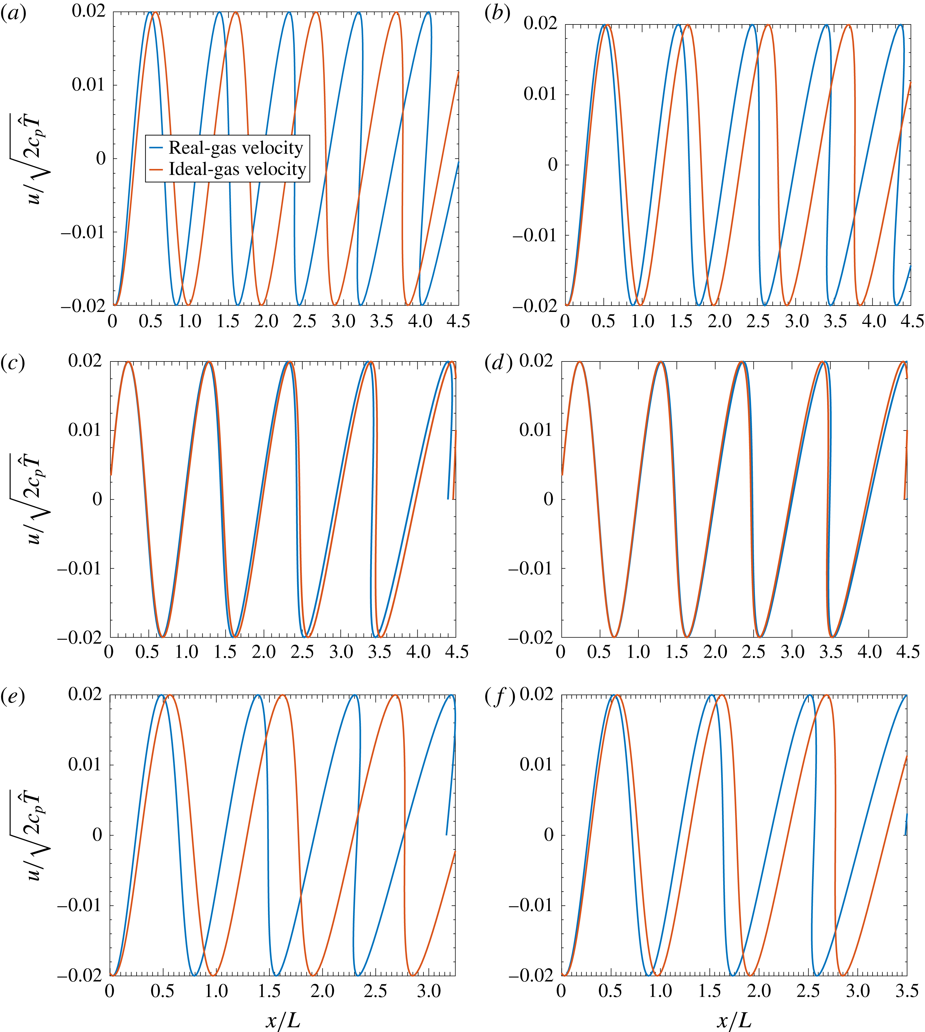
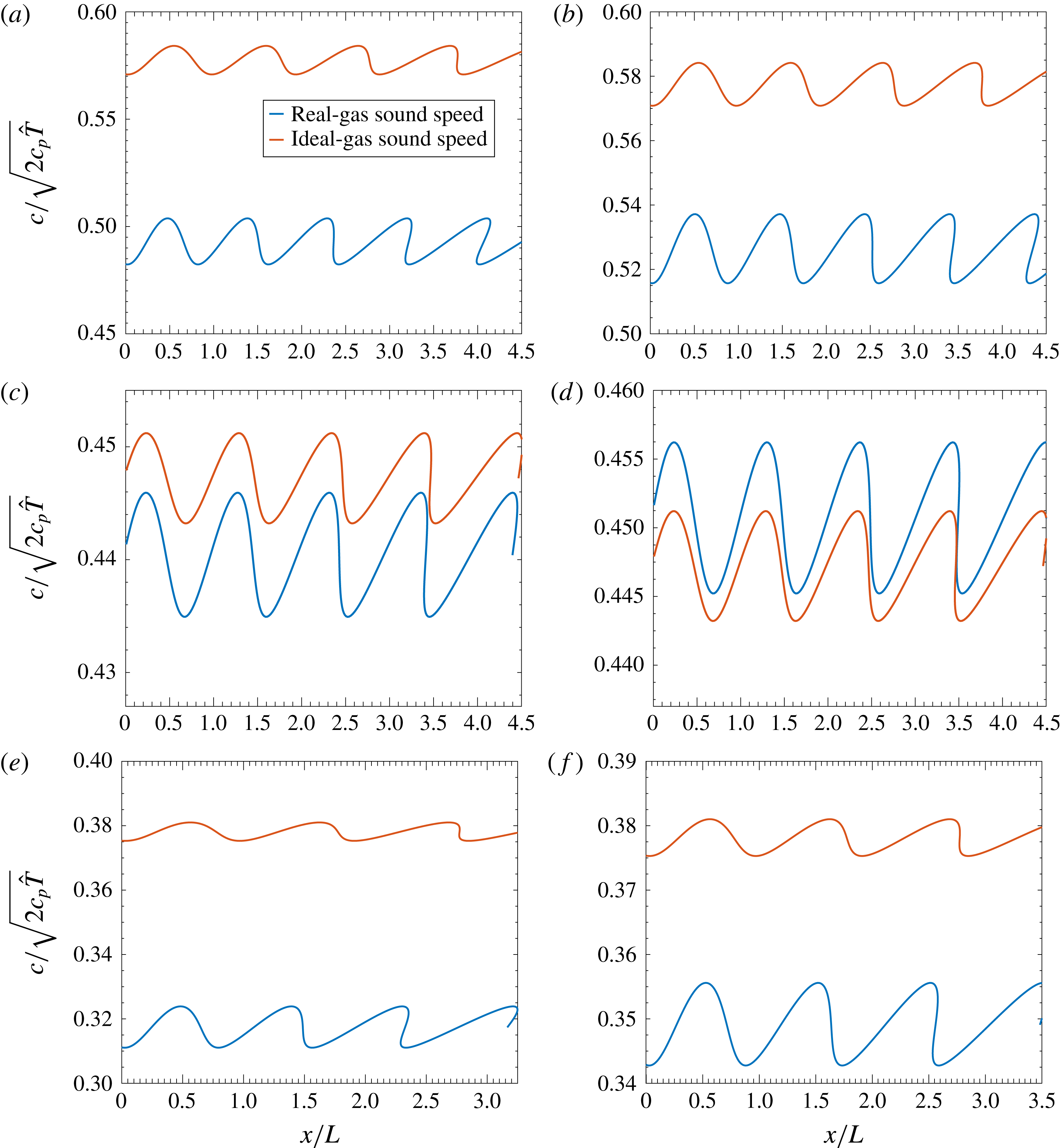
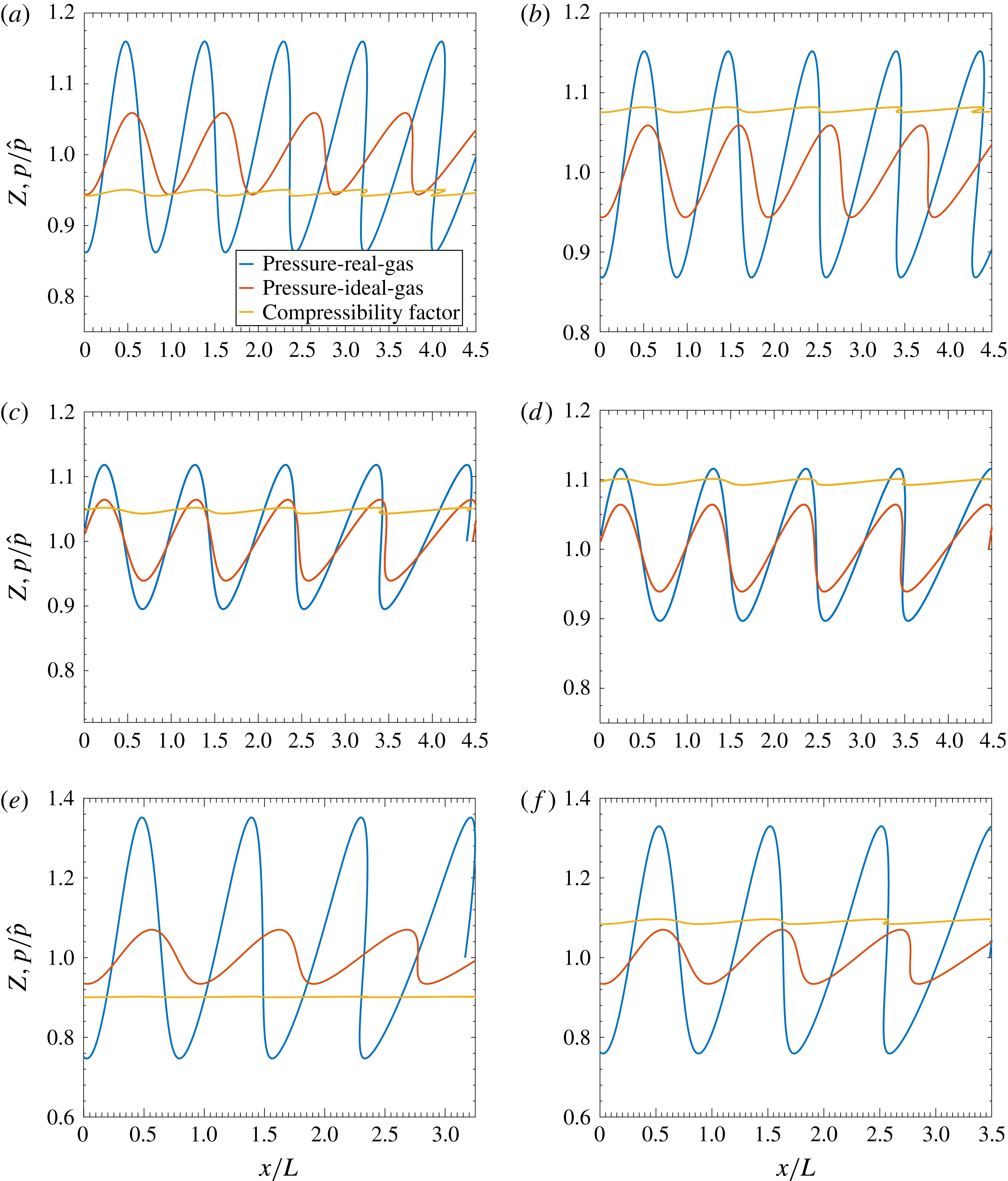
Results are presented in figures 5–7 for the same gases and stagnation conditions that were considered in the nozzle flow analysis. Non-dimensional velocity, sound speed and pressure versus non-dimensional spatial location are given for both the ideal-gas and real-gas calculations at a time $t^{\prime }=10$ , which is roughly the time for a wave to travel four to six wavelengths. (The non-dimensional frequency increases with $\unicode[STIX]{x1D6FE}$ here.) The non-dimensional velocity amplitude of the piston is given as $U=0.02$ , which is roughly 15–30 times smaller than the speed of sound, depending on the temperature. With the normalization scheme, the results easily scale to any frequency of piston oscillation. Generally, the original sinusoidal waveform distorts in well-known fashion towards an N-shaped waveform; multi-valued solutions are allowed to develop in physical space to emphasize the wave distortion; of course, a shock discontinuity must form, leaving only single-valued solutions.

Velocity is shown in figure 5. The same amplitude is maintained and is determined by the amplitude of piston motion for all cases. The ideal-gas and real-gas solutions for $u(\unicode[STIX]{x1D702})$ are identical sinusoidal functions, but solutions for $u(t^{\prime },x^{\prime })$ differ because the sound speeds differ. The real-gas wave generally moves slower than the ideal-gas wave. A modest exception occurs with nitrogen at the higher temperature. Ideal gases with higher $\unicode[STIX]{x1D6FE}$ and lower molecular mass tend to move more wavelengths as expected. The real gas does not follow the same trend. The differences between real and ideal behaviour is greater for carbon dioxide and argon than for nitrogen.

Figure 5.

Comparison of non-dimensional velocity for piston-driven flow between real-gas flow and ideal-gas flow: (a) argon, 300 K, 10 MPa; (b) argon, 1000 K, 30 MPa; (c) nitrogen, 400 K, 12 MPa; (d) nitrogen, 1000 K, 30 MPa; (e) carbon dioxide, 450 K, 10 MPa; (f) carbon dioxide, 1000 K, 30 MPa.

In figure 6, modest to profound differences in sound speed from the ideal-gas behaviour are seen. At lower temperatures, especially for carbon dioxide, the average real-gas sound speed is lower than the average ideal-gas value. At higher temperatures, the nitrogen real gas has a modestly higher sound speed. The real-gas sound speed amplitudes are generally higher than the ideal-gas amplitudes. The explanation follows from the facts that the $\unicode[STIX]{x1D6F9}$ function is negative and it oscillates out of phase with the velocity and sound speed. Thus, $\unicode[STIX]{x1D6F9}$ has a positive contribution in (5.17), thereby increasing the value of $c^{\prime }$ amplitude above the ideal-gas value.

Figure 6.

Comparison of non-dimensional sound speed for piston-driven flow between real-gas flow and ideal-gas flow: (a) argon, 300 K, 10 MPa; (b) argon, 1000 K, 30 MPa; (c) nitrogen, 400 K, 12 MPa; (d) nitrogen, 1000 K, 30 MPa; (e) carbon dioxide, 450 K, 10 MPa; (f) carbon dioxide, 1000 K, 30 MPa.

Figure 7 shows that the real-gas pressure has the most profound differences from the ideal gas; pressure amplitude is substantially increased at all temperatures but especially for the lower-temperature carbon dioxide, where an approximate tripling and doubling of the ideal-gas pressure amplitude case occurs at certain temperatures. Through the Riemann invariant, the velocity $u$ and sound speed $c$ are related linearly for the ideal gas and with a weakly nonlinear relation for the real gas. Consequently, the magnitudes of their amplitudes are comparable. However, the relation between pressure and sound speed involves a power law with exponent $2\unicode[STIX]{x1D6FE}/(\unicode[STIX]{x1D6FE}-1)$ , which affects the triatomic gas more than the diatomic gas (and in turn more than the monatomic gas). This power relation not only makes pressure amplitudes larger than other amplitudes for both the ideal and real gases, but also accentuates the difference between real and ideal gases. A higher pressure amplitude for the larger molecules is needed to achieve the amplitude of sound speed (or effectively the temperature and enthalpy amplitudes) demanded through the Riemann invariant by the magnitude of piston velocity, that is, the higher specific heat requires that the piston do more work raising the needed product of pressure and velocity.

Figure 7.

Comparison of non-dimensional pressure for piston-driven flow between real-gas flow and ideal-gas flow: (a) argon, 300 K, 10 MPa; (b) argon, 1000 K, 30 MPa; (c) nitrogen, 400 K, 12 MPa; (d) nitrogen, 1000 K, 30 MPa; (e) carbon dioxide, 450 K, 10 MPa; (f) carbon dioxide, 1000 K, 30 MPa.

The magnitudes of $Z-1$ , which capture the difference between real and ideal gases, are significant. The compressibility factor is seen in figure 7 to increase generally with temperature for these gases with values below one found for argon and carbon dioxide at lower temperatures. The amplitude of oscillation is more modest than found for other variables.

The author is unaware of previously published modifications to Riemann invariants owing to real-gas EoS effects.

6.1 Modified Prandtl relation

It is apparent that, for the ideal gas where $\unicode[STIX]{x1D701}_{1}=\unicode[STIX]{x1D701}_{2}=0$ , the enthalpy term in the energy conservation equation is easily related to the pressure term in the normal-momentum conservation equation. However, a more complex relation exists for a real gas. Using the energy equation to substitute into the pressure term of the momentum equation, it follows that

(6.6) $$\begin{eqnarray}\displaystyle \left[\frac{\unicode[STIX]{x1D6FE}+1}{\unicode[STIX]{x1D6FE}-1}\frac{c^{\ast 2}}{u_{1}}-u_{1}\right]\frac{1}{1+\unicode[STIX]{x1D701}_{1}}+\frac{2\unicode[STIX]{x1D6FE}}{\unicode[STIX]{x1D6FE}-1}u_{1}=\left[\frac{\unicode[STIX]{x1D6FE}+1}{\unicode[STIX]{x1D6FE}-1}\frac{c^{\ast 2}}{u_{2}}-u_{2}\right]\frac{1}{1+\unicode[STIX]{x1D701}_{2}}+\frac{2\unicode[STIX]{x1D6FE}}{\unicode[STIX]{x1D6FE}-1}u_{2}. & & \displaystyle\end{eqnarray}$$

After multiplying the left $c^{\ast 2}$ by $u_{2}/u_{2}$ and the right $c^{\ast 2}$ by $u_{1}/u_{1}$ , expanding with the small values of $\unicode[STIX]{x1D701}_{1}$ and $\unicode[STIX]{x1D701}_{2}$ , and factoring out $u_{2}-u_{1}$ , the relation becomes

(6.7) $$\begin{eqnarray}\displaystyle 1=\frac{c^{\ast 2}}{u_{1}u_{2}}\left[1-\frac{\unicode[STIX]{x1D701}_{1}u_{2}-\unicode[STIX]{x1D701}_{2}u_{1}}{u_{2}-u_{1}}\right]-\frac{\unicode[STIX]{x1D6FE}-1}{\unicode[STIX]{x1D6FE}+1}\,\frac{\unicode[STIX]{x1D701}_{2}u_{2}-\unicode[STIX]{x1D701}_{1}u_{1}}{u_{2}-u_{1}}. & & \displaystyle\end{eqnarray}$$

To lowest order, the classical Prandtl relation $c^{\ast 2}=u_{1}u_{2}$ is obtained and may be used to substitute into the higher-order term, yielding

(6.8) $$\begin{eqnarray}\displaystyle \frac{c^{\ast 2}}{u_{1}u_{2}}=1+\frac{\unicode[STIX]{x1D701}_{1}u_{2}-\unicode[STIX]{x1D701}_{2}u_{1}}{u_{2}-u_{1}}+\frac{\unicode[STIX]{x1D6FE}-1}{\unicode[STIX]{x1D6FE}+1}\,\frac{\unicode[STIX]{x1D701}_{2}u_{2}-\unicode[STIX]{x1D701}_{1}u_{1}}{u_{2}-u_{1}}. & & \displaystyle\end{eqnarray}$$

Consistently with the approximation here, $u_{2}=c^{\ast 2}/u_{1}$ may be substituted on the right-hand side of this equation to yield the modified Prandtl shock relation for high-pressure environments:

(6.9) $$\begin{eqnarray}\displaystyle \frac{c^{\ast 2}}{u_{1}u_{2}}=1+\frac{\unicode[STIX]{x1D701}_{1}c^{\ast 2}-\unicode[STIX]{x1D701}_{2}u_{1}^{2}}{c^{\ast 2}-u_{1}^{2}}+\frac{\unicode[STIX]{x1D6FE}-1}{\unicode[STIX]{x1D6FE}+1}\,\frac{\unicode[STIX]{x1D701}_{2}c^{\ast 2}-\unicode[STIX]{x1D701}_{1}u_{1}^{2}}{c^{\ast 2}-u_{1}^{2}}. & & \displaystyle\end{eqnarray}$$

In some cases, numerical difficulties occur with the form of (6.9) because some of the terms on the right-hand side occasionally involve the ratio of two small numbers. It becomes more convenient at times to solve (6.6) as a quadratic equation for $u_{2}$ , using the negative-sign option in the classical formula and iterating to update volumes of  $\unicode[STIX]{x1D701}_{2}$ .

For the limit of the ideal gas, the classical $c^{\ast 2}=u_{1}u_{2}$ is recovered and, in the limit of shock strength going to zero for the ideal gas, $c^{\ast }=u_{1}=u_{2}=c$ . This is not the general real-gas result; $c^{\ast 2}$ remains proportional to the stagnation enthalpy but the relation with velocity is more complex.

The limiting characteristic velocity value can be determined as the strength of the shock wave goes to zero, i.e.  $u_{2}\rightarrow u_{1}$ . Equations (6.1) and (6.9) are used with the definition of $c^{\ast }$ to obtain

(6.10) $$\begin{eqnarray}c^{\ast 2}=\left[1+\frac{2\unicode[STIX]{x1D6FE}}{\unicode[STIX]{x1D6FE}+1}\unicode[STIX]{x1D701}_{1}\right]u_{1}^{2}=2\frac{\unicode[STIX]{x1D6FE}-1}{\unicode[STIX]{x1D6FE}+1}{\hat{h}}_{1}=2\frac{\unicode[STIX]{x1D6FE}-1}{\unicode[STIX]{x1D6FE}+1}\left[h_{1}+\frac{u_{1}^{2}}{2}\right],\end{eqnarray}$$

(6.11) $$\begin{eqnarray}\displaystyle u_{1}^{2} & = & \displaystyle \frac{(\unicode[STIX]{x1D6FE}-1)h_{1}}{1+\unicode[STIX]{x1D6FE}\unicode[STIX]{x1D701}_{1}}\approx (\unicode[STIX]{x1D6FE}-1)h_{1}(1-\unicode[STIX]{x1D6FE}\unicode[STIX]{x1D701}_{1})\nonumber\\ \displaystyle & = & \displaystyle \frac{\unicode[STIX]{x1D6FE}p_{1}}{\unicode[STIX]{x1D70C}_{1}}(1+\unicode[STIX]{x1D701}_{1})(1-\unicode[STIX]{x1D6FE}\unicode[STIX]{x1D701}_{1})\approx \frac{\unicode[STIX]{x1D6FE}p_{1}}{\unicode[STIX]{x1D70C}_{1}}[1-(\unicode[STIX]{x1D6FE}-1)\unicode[STIX]{x1D701}_{1}].\end{eqnarray}$$

This limiting velocity for the real gas is generally not the characteristic velocity. In particular, $c^{\ast }$ does not go to $c_{1}$ as shock strength goes to zero. Here $\unicode[STIX]{x1D701}$ is the fractional departure of $(\unicode[STIX]{x1D6FE}-1)h$ from $\unicode[STIX]{x1D6FE}p/\unicode[STIX]{x1D70C}$ and $-(\unicode[STIX]{x1D6FE}-1)\unicode[STIX]{x1D701}_{1}/2$ is the fractional departure of the limiting wave speed from $\sqrt{\unicode[STIX]{x1D6FE}p_{1}/\unicode[STIX]{x1D70C}_{1}}.$ Thus, $[Z_{1}-1-(\unicode[STIX]{x1D6FE}-1)\unicode[STIX]{x1D701}_{1}]/2$ is the fractional departure of the limiting wave speed from $\sqrt{\unicode[STIX]{x1D6FE}RT_{1}}.$ When the attraction parameter $A_{1}$ becomes larger (smaller) than the repulsion parameter $B_{1}$ , $Z_{1}-1$ becomes negative (positive) but $\unicode[STIX]{x1D701}_{1}$ tends towards becoming positive (negative). The change in sign does not occur simultaneously for $\unicode[STIX]{x1D701}$ and $Z-1$ . Nevertheless, real-gas limiting wave speed tends to be larger (smaller) than the ideal-gas value when $B_{1}>A_{1}$ ( $B_{1}<A_{1}$ ).

An interesting set of normal shock calculations for real-gas flow of air at upstream values $T_{1}=700$  K, $p_{1}=1$ , 4 and 50 MPa is given by Kouremenos & Antonopoulos (Reference Kouremenos and Antonopoulos1989). They use the original Redlich–Kwong form of the EoS but qualitative differences are not expected with our SRK form. Results are reported for the range $1.2\leqslant M_{1}\leqslant 5.5$ . That paper makes no mention of a modified Prandtl relation or modified Rankine–Hugoniot relation.

6.2 Modified Rankine–Hugoniot relation

Next, the modifications of the Rankine–Hugoniot relation are examined by manipulation of the conservation laws of (6.5). Combination of the normal-momentum and continuity relations yields

(6.12a,b ) $$\begin{eqnarray}\displaystyle u_{1}^{2}=\frac{p_{2}-p_{1}}{\unicode[STIX]{x1D70C}_{2}-\unicode[STIX]{x1D70C}_{1}}\frac{\unicode[STIX]{x1D70C}_{2}}{\unicode[STIX]{x1D70C}_{1}},\quad u_{2}^{2}=\frac{p_{2}-p_{1}}{\unicode[STIX]{x1D70C}_{2}-\unicode[STIX]{x1D70C}_{1}}\frac{\unicode[STIX]{x1D70C}_{1}}{\unicode[STIX]{x1D70C}_{2}}. & & \displaystyle\end{eqnarray}$$

Substitution for the velocity terms in the energy equation and multiplication by the factor $\unicode[STIX]{x1D70C}_{1}/p_{1}$ gives a linear relation for the pressure ratio $p_{2}/p_{1}$ in terms of $\unicode[STIX]{x1D70C}_{2}/\unicode[STIX]{x1D70C}_{1},~\unicode[STIX]{x1D6FE},~\unicode[STIX]{x1D701}_{1}$ and $\unicode[STIX]{x1D701}_{2}$ . Solution of that linear relation yields the modified Rankine–Hugoniot relation:

(6.13) $$\begin{eqnarray}\displaystyle \frac{p_{2}}{p_{1}}=\left[\frac{\unicode[STIX]{x1D70C}_{2}}{\unicode[STIX]{x1D70C}_{1}}-\frac{\unicode[STIX]{x1D6FE}-1}{\unicode[STIX]{x1D6FE}+1+2\unicode[STIX]{x1D6FE}\unicode[STIX]{x1D701}_{1}}\right]\left[1-\frac{\unicode[STIX]{x1D6FE}-1}{\unicode[STIX]{x1D6FE}+1+2\unicode[STIX]{x1D6FE}\unicode[STIX]{x1D701}_{2}}\frac{\unicode[STIX]{x1D70C}_{2}}{\unicode[STIX]{x1D70C}_{1}}\right]^{-1}. & & \displaystyle\end{eqnarray}$$

Equations (6.9) and (6.13) give the classical Prandtl and Rankine–Hugoniot relations when $\unicode[STIX]{x1D701}_{1}=\unicode[STIX]{x1D701}_{2}=0$ . Solutions to the modified relations can readily be obtained in a two-step iteration. First, taking $\unicode[STIX]{x1D701}_{1}=\unicode[STIX]{x1D701}_{2}=0$ and given upstream values for $u_{1},~v_{1},~p_{1}$ and $\unicode[STIX]{x1D70C}_{1}$ , equations (6.9) and (6.13), together with transverse-momentum and continuity equations in (6.5), yield the zeroth-order approximations to the downstream values, i.e.  $u_{2}^{\ast },~p_{2}^{\ast }$ and $\unicode[STIX]{x1D70C}_{2}^{\ast }$ and the correct value for $v_{2}$ . Next, using these values for $p_{2}^{\ast }$ and $\unicode[STIX]{x1D70C}_{2}^{\ast }$ with the ideal-gas relation, the values of $T_{2}^{\ast }$ and $\unicode[STIX]{x1D701}_{2}$ are determined with sufficient accuracy. Substitution of $\unicode[STIX]{x1D701}_{1}$ and $\unicode[STIX]{x1D701}_{2}$ into (6.9), (6.13) and the continuity equation gives $u_{2},~p_{2}$ and $\unicode[STIX]{x1D70C}_{2}$ with the desired accuracy. Then, $T_{2}$ is determined from $Z=1+B-A$ and $h_{2}={\hat{h}}-(u_{2}^{2}+v_{2}^{2})/2.$

As the pressure ratio $p_{2}/p_{1}\rightarrow \infty$ in (6.13), it follows that

(6.14) $$\begin{eqnarray}\displaystyle \left.\begin{array}{@{}c@{}}\displaystyle \frac{\unicode[STIX]{x1D70C}_{2}}{\unicode[STIX]{x1D70C}_{1}}\rightarrow \frac{\unicode[STIX]{x1D6FE}+1+2\unicode[STIX]{x1D6FE}\unicode[STIX]{x1D701}_{2}}{\unicode[STIX]{x1D6FE}-1},\\ \displaystyle \unicode[STIX]{x1D701}_{2}=\frac{2-\unicode[STIX]{x1D6FE}}{\unicode[STIX]{x1D6FE}}A-\frac{1}{\unicode[STIX]{x1D6FE}}B+\frac{\unicode[STIX]{x1D6FE}-1}{\unicode[STIX]{x1D6FE}}A^{\prime }\rightarrow \frac{1}{\unicode[STIX]{x1D6FE}}\left[\frac{\tilde{a}S^{2}}{R_{u}T_{c}}-b\right]\frac{p_{2}}{R_{u}T_{2}}=\frac{1}{\unicode[STIX]{x1D6FE}}\left[\frac{\tilde{a}S^{2}}{R_{u}T_{c}}-b\right]\frac{\unicode[STIX]{x1D70C}_{2}}{W}.\end{array}\right\}\qquad & & \displaystyle\end{eqnarray}$$

In the limits for $A$ and $A^{\prime }$ , it has been considered that temperature ratio goes to infinity as pressure ratio goes to infinity. For the ideal gas, $(\unicode[STIX]{x1D70C}_{2}/\unicode[STIX]{x1D70C}_{1})|_{ideal}\rightarrow (\unicode[STIX]{x1D6FE}+1)/(\unicode[STIX]{x1D6FE}-1)$ , giving a finite limiting value for $\unicode[STIX]{x1D70C}_{2}$ . Thus, $\unicode[STIX]{x1D701}_{2}$ has a finite limit, thereby yielding, for the real gas, the finite limit

(6.15) $$\begin{eqnarray}\displaystyle \left.\frac{\unicode[STIX]{x1D70C}_{2}}{\unicode[STIX]{x1D70C}_{1}}\right|_{real}\rightarrow \frac{\displaystyle \unicode[STIX]{x1D6FE}+1+2\left[\frac{\tilde{a}S^{2}}{R_{u}T_{c}}-b\right]}{\unicode[STIX]{x1D6FE}-1}\frac{\unicode[STIX]{x1D70C}_{2}}{W}=\left(1+2\frac{\unicode[STIX]{x1D70C}_{1}}{W(\unicode[STIX]{x1D6FE}-1)}\left[\frac{\tilde{a}S^{2}}{R_{u}T_{c}}-b\right]\right)\frac{\unicode[STIX]{x1D6FE}+1}{\unicode[STIX]{x1D6FE}-1}.\qquad & & \displaystyle\end{eqnarray}$$

Differentiation of $p_{2}$ given by (6.13) with respect to $\unicode[STIX]{x1D70C}_{2}$ , holding upstream values constant, and taking the limit as $p_{2}\rightarrow p_{1}$ , yields the result

(6.16) $$\begin{eqnarray}\displaystyle \left.\frac{\text{d}p_{2}}{\text{d}\unicode[STIX]{x1D70C}_{2}}\right|_{p_{2}\rightarrow p_{1}}=\frac{\unicode[STIX]{x1D6FE}p_{1}}{\unicode[STIX]{x1D70C}_{1}}\left[\left.1-(\unicode[STIX]{x1D6FE}-1)\unicode[STIX]{x1D701}_{1}-\frac{\unicode[STIX]{x1D6FE}-1}{\unicode[STIX]{x1D6FE}+1}\unicode[STIX]{x1D70C}_{1}\frac{\text{d}\unicode[STIX]{x1D701}_{2}}{\text{d}\unicode[STIX]{x1D70C}_{2}}\right|_{p_{2}\rightarrow p_{1}}\right]. & & \displaystyle\end{eqnarray}$$

The derivative $\text{d}\unicode[STIX]{x1D701}_{2}/\text{d}\unicode[STIX]{x1D70C}_{2}$ in (6.16) is taken along the path $p_{2}(\unicode[STIX]{x1D70C}_{2})$ defined by (6.13). Specifically, $\unicode[STIX]{x1D701}_{2}$ taken from (6.1) should be cast as $\unicode[STIX]{x1D701}_{2}(p_{2},\unicode[STIX]{x1D70C}_{2})$ . The derivative of $\unicode[STIX]{x1D701}_{2}$ involves both the explicit derivative and the implicit derivative through $p_{2}(\unicode[STIX]{x1D70C}_{2})$ . For the latter derivative, the approximate form $(\text{d}p_{2}/\text{d}\unicode[STIX]{x1D70C}_{2})|_{p_{2}\rightarrow p_{1}}=\unicode[STIX]{x1D6FE}p_{1}/\unicode[STIX]{x1D70C}_{1}$ suffices in this higher-order term. As known, for the ideal gas, in this limit of shock strength going to zero, the derivative along the Rankine–Hugoniot curve given by (6.16) goes to the value for the derivative along the isentropic particle path in that limiting situation, namely, $(\text{d}p_{2}/\text{d}\unicode[STIX]{x1D70C}_{2})|_{p_{2}\rightarrow p_{1}}\rightarrow \unicode[STIX]{x1D6FE}p_{1}/\unicode[STIX]{x1D70C}_{1}=c^{2}=(\unicode[STIX]{x2202}p_{2}/\unicode[STIX]{x2202}\unicode[STIX]{x1D70C}_{2})|_{s}$ . For the general case of the real gas, this tangency also occurs.

The entropy gain across the shock is of third order in non-dimensional pressure gain for an ideal gas. This means that, in the limiting behaviour of a weak shock, $T\,\text{d}s=\text{d}h-(1/\unicode[STIX]{x1D70C})\,\text{d}p\ll \text{d}h\approx (1/\unicode[STIX]{x1D70C})\,\text{d}p$ along the direct integration path (monotonic variations) from upstream to downstream conditions. A second-order-accurate measure of this condition can be created using the mean-value theorem. Namely, the magnitude of $\unicode[STIX]{x1D6E5}\equiv (\unicode[STIX]{x1D70C}_{1}/p_{1})[h_{2}-h_{1}]-2[p_{2}/p_{1}-1]/[\unicode[STIX]{x1D70C}_{2}/\unicode[STIX]{x1D70C}_{1}+1]$ can be compared to the magnitude of $(\unicode[STIX]{x1D70C}_{1}/p_{1})[h_{2}-h_{1}]$ (or $2[p_{2}/p_{1}-1]/[\unicode[STIX]{x1D70C}_{2}/\unicode[STIX]{x1D70C}_{1}+1]$ ).

6.3 Shock results

Results for two cases with nitrogen gas are examined in figures 8 and 9, with upstream flow values for temperature and pressure given by 400 K, 10 MPa and 300 K, 3 MPa, respectively. These examples involve upstream conditions at supercritical pressure and supercritical temperature and at subcritical pressure and supercritical temperature, respectively. An attempt is made to choose upstream values that keep errors due to linearization small in the downstream flow. Among other things, this disallows treatment of compressible liquids at supercritical pressures and subcritical temperatures. Nitrogen is favoured because it has the lowest critical values of the gases selected here for computations in other sections; thereby the upstream pressure and temperature are taken at sufficiently low values to keep the $A$ and $B$ parameters behind the shock low enough to validate the linearization.

Calculations are made over a range of $u_{1}$ values and displayed in figures 8 and 9. Some portions of the range are not physically reasonable since the second law of thermodynamics is not reflected in the algorithms. For example, portions of the curves where ratios of pressure, density, temperature and enthalpy drop below values of one have been disregarded and are not shown in the figures.

Significant differences in the Rankine–Hugoniot (RH) plots are generally seen in figures 8(a) and 9(a). The largest differences in pressure ratio between the real gas and the ideal gas occur near the limiting density ratios, which themselves differ substantially. In these cases, the real gas has a smaller value for the upper limit on density ratio. Both the real and ideal cases are each calculated in two ways as an error estimate on the linearization: (i) downstream pressure and density are calculated and then the ratios are ‘directly’ formed; and (ii) the RH formula is calculated. The error is small enough to make useful conclusions. Figures 8(a) and 9(a) and other results not shown here indicate that the real-gas pressure ratio generally appears larger (smaller) than the ideal-gas ratio when $B>A~(A>B)$ . (This should not be taken as a strict rule, since quantities such as $A^{\prime }$ and $A^{\prime \prime }$ can have an influence.) At some values of density ratio, the RH results from figures 8(a) and 9(a) show very large differences in pressure ratio between the ideal gas and the real gas; in particular, the real-gas shock is much stronger there. This behaviour is consistent with the results for the continuous wave given in figure 7, where real gases had larger pressure amplitudes for the same forcing mechanism; the continuous waves there are expected to deform to N-shaped waveforms with shock formation. Note however that, at the same shock velocity $u_{1}$ , the ideal gas can yield the greater pressure ratio as shown in figures 8(b) and 9(b). The velocity ratio, however, will be given as the reciprocal of the density ratio; thus the fractional change in velocity is smaller for the real gas in these cases.

Figure 8.

Shock wave – comparison of non-dimensional solutions between real gas and ideal gas for nitrogen, at $T_{1}=400$  K,  $p_{1}=10~\text{MPa}$ , $u_{1}=400{-}2500~\text{m}~\text{s}^{-1}$ : (a) Rankine–Hugoniot relation; (b) pressure ratio versus shock velocity; (c) enthalpy and temperature ratios; (d) upstream and downstream Mach numbers; (e) compressibility factor $Z$ , attraction parameter $A$ , repulsion parameter $B$ ; (f) non-dimensional shock jumps in pressure, entropy and enthalpy, and $M_{2}-1$ .

Figure 9.

Shock wave – comparison of non-dimensional solutions between real gas and ideal gas for nitrogen, at $T_{1}=300$  K,  $p_{1}=3~\text{MPa}$ , $u_{1}=350{-}2000~\text{m}~\text{s}^{-1}$ : (a) Rankine–Hugoniot relation; (b) pressure ratio versus shock velocity; (c) enthalpy and temperature ratios; (d) upstream and downstream Mach numbers; (e) compressibility factor $Z$ , attraction parameter $A$ , repulsion parameter $B$ ; (f) non-dimensional shock jumps in pressure, entropy and enthalpy, and $M_{2}-1$ .

Enthalpy and temperature show differences for the real gas in figures 8(c) and 9(c); downstream ideal-gas temperature exceeds real-gas temperature for the same shock velocity. Generally, non-dimensional enthalpy exceeds non-dimensional temperature for the real gas. Figures 8(d) and 9(d) show that, for the given upstream conditions, the shock Mach number is smaller for the real gas. Figures 8(e) and 9(e) show that a portion of the domain has the values of $A$ and $B$ within desirable constraints for accuracy; however, for other portions, they achieve magnitudes near 0.4, which raises our error estimates to above 10 %.

Figure 8(f) shows the results for nitrogen at upstream values of 400 K, 10 MPa. In similar fashion to the previous example in the same figure, an inflow velocity of approximately $450~\text{m}~\text{s}^{-1}$ , $p_{2}\rightarrow p_{1},~\unicode[STIX]{x1D70C}_{2}\rightarrow \unicode[STIX]{x1D70C}_{1},~h_{2}\rightarrow h_{1},~T_{2}\rightarrow T_{1}$ and $Z_{2}\rightarrow Z_{1}$ are found. Figure 8(f) also shows that the approximate measure $\unicode[STIX]{x1D6E5}$ related to entropy change is going to the zero limit and is higher order in magnitude.

The low-temperature nitrogen case is examined through figure 9. Here, the limiting behaviour presents no surprises. At an inflow velocity of $357~\text{m}~\text{s}^{-1}$ , $p_{2}\rightarrow p_{1},~\unicode[STIX]{x1D70C}_{2}\rightarrow \unicode[STIX]{x1D70C}_{1},~h_{2}\rightarrow h_{1},~T_{2}\rightarrow T_{1},~Z_{2}\rightarrow Z_{1}$ and $M_{2}\rightarrow M_{1}\rightarrow 1$ . Within our error here, $Z_{1}=1$ ; the limit should show ideal-gas behaviour. In the calculations here (including unpublished cases), no cases with $M_{1}<1$ and entropy gain were found; they should be physically unstable if they exist as mathematical solutions.

Some analytical support can be given for the finding of limiting velocities not at the sonic speed. The relation between enthalpy and sound from (C 16) and (6.1) yields

(6.17) $$\begin{eqnarray}\displaystyle \unicode[STIX]{x1D6FE}\frac{p}{\unicode[STIX]{x1D70C}}=\frac{c^{2}}{1+\unicode[STIX]{x1D70E}}=\frac{(\unicode[STIX]{x1D6FE}-1)h}{1+\unicode[STIX]{x1D701}}, & & \displaystyle\end{eqnarray}$$

and thus

(6.18) $$\begin{eqnarray}\displaystyle h\approx \frac{c^{2}}{\unicode[STIX]{x1D6FE}-1}[1+\unicode[STIX]{x1D701}-\unicode[STIX]{x1D70E}]. & & \displaystyle\end{eqnarray}$$

The energy conservation across the shock may be developed as follows and combined with the momentum relation:

(6.19) $$\begin{eqnarray}\displaystyle \left.\begin{array}{@{}c@{}}\displaystyle h_{2}-h_{1}=\frac{u_{1}^{2}-u_{2}^{2}}{2}=\frac{u_{1}+u_{2}}{2}(u_{1}-u_{2}),\\ \displaystyle \unicode[STIX]{x1D6FF}h=\left.\frac{u_{1}+u_{2}}{2\unicode[STIX]{x1D70C}_{1}u_{1}}\right|_{u_{2}\rightarrow u_{1}}\unicode[STIX]{x1D6FF}p\rightarrow \frac{1}{\unicode[STIX]{x1D70C}_{1}}\unicode[STIX]{x1D6FF}p.\end{array}\right\} & & \displaystyle\end{eqnarray}$$

The definitions $\unicode[STIX]{x1D6FF}h=h_{2}-h_{1},~\unicode[STIX]{x1D6FF}u=u_{2}-u_{1}$ , etc. are applied in the limit as the jump across the shock is disappearing. As the jump across the shock becomes small, the asymptote is giving an isentropic result as shown by comparison with the differential relation that describes the combined first and second laws, i.e.  $T\,\text{d}s=\text{d}h-(1/\unicode[STIX]{x1D70C})\,\text{d}p$ .

Table 4 compares present approximate calculations with the cubic-equation computations of Kouremenos & Antonopoulos (Reference Kouremenos and Antonopoulos1989), now designated as KA. Ratios of pressure and temperature plus downstream Mach number are compared for certain upstream Mach numbers. Subscripts $KA$ and $S$ are used in the table for the results of Kouremenos & Antonopoulos (Reference Kouremenos and Antonopoulos1989) and the current results, respectively. The KA computations were done for a normal shock in air using the Redlich–Kwong EoS, while the S results treat a normal shock in nitrogen and use the linearized SRK EoS. The quantitative KA results were interpreted from their graph (Kouremenos & Antonopoulos Reference Kouremenos and Antonopoulos1989, figure 2); so, the number of trusted significant digits was limited. They made no comparison with ideal-gas results. Table 4 shows that KA and S results compare favourably. For the chosen range of $M_{1}$ , $Z_{2}$ varied from 1.02 to 1.06 in the S results, increasing with $M_{1}$ ; and the downstream pressure, temperature and density were each lower than the value yielded for the ideal gas, with the difference increasing with $M_{1}$ . The KA article also had results for 50 MPa, which yields too high a value of $Z_{2}-1$ to apply our linearization and make a useful comparison; $Z_{2}=1.2$ and higher downstream.

Table 4.

Comparison with Kouremenos & Antonopoulos (Reference Kouremenos and Antonopoulos1989) normal shock calculations. Values for upstream Mach number, downstream Mach number, temperature ratio and pressure ratio. Upstream values were 700 K and 4 MPa.