1. Introduction
Questions concerning explanation, prediction, and control in the sciences are oftentimes answered by pointing at the system of interest’s underlying mechanism and showing how causal interactions of this mechanism’s parts bring about the phenomenon of interest. Mechanisms are typically characterized qualitatively. Glennan (Reference Glennan1996), for example, defines a mechanism underlying a behavior as a “complex system which produces that behavior by of the interaction of a number of parts according to direct causal laws” (52). (For other prominent characterizations see, e.g., Machamer, Darden, and Craver [Reference Machamer, Darden and Craver2000, 3] or Bechtel and Abrahamsen [Reference Bechtel and Abrahamsen2005, 423]).
For providing quantitatively precise mechanistic explanation/prediction and answering questions concerning the results of manipulations, however, a formal representation of mechanisms is required. Casini et al. (Reference Casini, lllari, Russo and Williamson2011) suggest to model mechanisms by means of recursive Bayesian networks (RBNs). Gebharter (Reference Gebharter2014) highlights two problems with Casini et al.’s approach and suggests the multilevel causal model (MLCM) approach as an alternative.Footnote 1 While Casini et al. represent mechanisms by a special kind of node of a Bayesian network (BN), Gebharter represents them by directed or bidirected causal arrows. The latter seems promising; it suggests, for example, to develop new methods for discovering submechanisms, that is, the causal structure inside the causal arrows (see, e.g., Murray-Watters and Glymour Reference Murray-Watters and Glymour2015). In addition, many results from the statistics and machine learning literature can be directly applied to models of mechanisms. Zhang (Reference Zhang2008), for example, shows how the effects of interventions can be computed in models featuring bidirected arrows, and Richardson (Reference Richardson, Bilmes and Ng2009) develops a factorization criterion equivalent to the d-connection condition for such models.
One of the shortcomings the RBN and the MLCM approach share is that they presuppose acyclicity, and thus, do not allow for a representation of mechanisms featuring feedback.Footnote 2 Clarke, Leuridan, and Williamson (Reference Clarke, Leuridan and Williamson2014) further develop the RBN approach in such a way that it can be applied to mechanisms featuring causal cycles. They distinguish between static and dynamic problems. Static problems are “situations in which a specific cycle reaches equilibrium … and where the equilibrium itself is of interest, rather than the process of reaching equilibrium.” A dynamic problem is a “situation in which it is the change in the values of variables over time that is of interest” (sec. 6). Clarke et al. suggest to solve static problems on the basis of the notion of d-separation (Pearl Reference Pearl2000, sec. 1.2.3) and dynamic problems by means of dynamic Bayesian networks (DBNs). In this article, we follow their example and demonstrate how the MLCM approach for representing mechanisms can be modified and extended in a similar way.
The article is structured as follows: in section 2 we introduce the causal modeling framework used in the article. In section 3 we give an overview of the MLCM approach. In sections 4.1 and 4.2 we demonstrate by means of a simple toy mechanism how the MLCM approach can be modified in such a way that it can be applied to static and dynamic problems, respectively. Both modifications mirror Clarke et al.’s (Reference Clarke, Leuridan and Williamson2014) suggestions for solving static and dynamic problems without sharing certain shortcomings.
2. Causal Nets
A causal net (or model) is a triple 〈V, E, P〉, where 〈V, E〉 is a directed graph providing causal information about the elements of V, V is a set of random variables, and E is a binary relation on V that is interpreted as direct causal connection relative to V. Set V’s elements are called the graph’s vertices, E’s elements its edges. And P is a probability distribution over V representing regularities produced by the causal structure underlying V.
Causal connections between variables are represented by directed and bidirected arrows: “X → Y” means that X is a direct cause of Y, and “X ↔ Y” means that X and Y are effects of a common cause not included in V. Causal models are assumed to not feature self-edges X → X or X ↔ X. The set of Y’s parents is  . A chain of n ≥ 1 edges (of any kind) connecting two variables X and Y is called a path between X and Y if it does not go through any variable more often than once. (Note that π’s being a path between X and Y allows that X = Y.) A path
 is called a directed path from X to Y; X is called a cause of Y and Y an effect of X. A variable Z lying on a path
 is called an intermediate cause lying on this path. A path
 is called a common cause path with Z as a common cause of X and Y lying on this path. A path connecting X and Y containing a subpath
 is called a collider path connecting X and Y, and Zj is called a collider lying on this path.Footnote 3 A path between X and Y indicates a common cause path if it either is a common cause path or a collider-free path that contains a bidirected edge. A path
 is called a causal cycle. A graph is called cyclic if it features causal cycles; it is called acyclic otherwise. Likewise for causal models.
For now we only require the causal net approach’s most central axiom, the causal Markov condition (CMC). A model 〈V, E, P〉 satisfies CMC if and only if (iff) every X ∈ V is probabilistically independent of its noneffects conditional on its direct causes (Spirtes, Glymour, and Scheines Reference Spirtes, Glymour and Scheines1993, 54). If an acyclic causal model satisfies CMC, then its graph determines the following Markov factorization (54):

3. The Multilevel Causal Model Approach
The MLCM approach is based on the simple idea that mechanisms are devices bringing about certain input-output behaviors (cf. Bechtel Reference Bechtel, Schouton and de Jong2007, sec. 3; Craver Reference Craver2007, 145). This suggests a representation of mechanisms by a causal model’s arrows. The variables at the arrows’ tails stand for the mechanism’s input, the variables at the arrows’ heads stand for the mechanism’s output, and the arrows represent the not-further-specified mechanism. A graph describing such a mechanism can be supplemented by a probability distribution P that quantitatively describes the system’s behavior.
Mechanistic explanation requires investigating how a mechanism produces the phenomenon of interest; it requires a more detailed description of the underlying causal structure producing that phenomenon. One can give such an explanation by supplementing a causal model M, whose graph’s arrows represent a mechanism, by another causal model M′ that contains new variables describing the behaviors of some parts of the mechanism. So, metaphorically speaking, we are “zooming” into the device represented by the arrows. However, it must be assured that the more detailed causal model M′ fits to the original model M with respect to its causal structure and its probability distribution. The following notion of a restriction states conditions for such a fit (Gebharter Reference Gebharter2014, 147):Footnote 4 is a restriction of
 iff
 ,
 ,Footnote 5 the following two conditions hold for all
 , and no path not implied by these conditions is in 〈V, E〉:
1. If there is a path from X to Y in 〈V′, E′〉 and no vertex on this path different from X and Y is in V, then X → Y in 〈V, E〉.
2. If X and Y are connected by a path π in 〈V′, E′〉 indicating a common cause path and no vertex on π different from X and Y is in V, then X ↔ Y in 〈V, E〉.
This notion tells us which causal models M′ are candidates for mechanistically explaining phenomena described by a less detailed model M. It also tells us how we can marginalize out variables from M′ while preserving information about the causal and probabilistic relationships among variables in V provided by M′. For a detailed motivation of this notion of a restriction, see Gebharter (Reference Gebharter2014, 147–48).
We can now define an MLCM as a structure  such that every causal model Mi with i > 1 is a restriction of M 1, while M 1 satisfies CMC (Gebharter Reference Gebharter2014, 148). The latter condition reflects a basic assumption of the causal nets approach, that is, that for explaining a probability distribution P, reference to an underlying causal structure satisfying CMC is required (cf. Spirtes et al. Reference Spirtes, Glymour and Scheines1993, sec. 6.1).Footnote 6
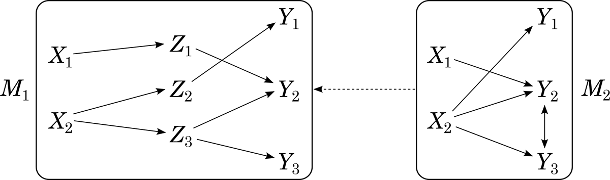
Let us briefly illustrate by means of figure 1 how MLCMs can be used for modeling mechanisms. Model M 2 describes the mechanism’s top level. The mechanism has two input variables (X 1, X 2) and three output variables (Y 1, Y 2, Y 3). The arrows stand for the not-further-specified mechanism. Mechanistic explanation of a certain phenomenon, for example, of an input-output behavior  , requires a more detailed story about what is happening within the mechanism, that is, within the system represented by the arrows. This story is told by M 1. Model M 1 features three new variables (Z 1, Z 2, Z 3) describing parts of the mechanism. Model M 1’s causal structure tells us over which causal paths through the mechanism X 1 and X 2 cause Y 1, Y 2, and Y 3. Model M 2 is a restriction of M 1. And M 1 is assumed to satisfy CMC.
Figure 1.

4. Modeling Mechanisms with Causal Cycles
We introduce the following toy mechanism for investigating the question of how to model mechanisms featuring causal cycles within the MLCM approach: a simple temperature regulation system, where OT stands for the outside temperature, IT for the inside temperature, and CK for a control knob. The behavior of interest is that IT is relatively insensitive to OT when CK = on, that is, that  for arbitrary OT and IT values.
A simple input-output representation of this mechanism would be a causal model M 2 with the graphical structure  . A mechanistic explanation of
 by means of an MLCM would require connecting M 2 to a more detailed model M 1 satisfying CMC. Since the system represented is a self-regulatory system, M 1 is expected to feature a cycle
 . But cyclic causal models do have some problems with CMC. While CMC can, in principle, be applied to cyclic causal models, it turns out to be inadequate. Let us illustrate this by means of the following example borrowed from Spirtes et al. (Reference Spirtes, Glymour and Scheines1993, 359): Suppose a causal model with the structure
 satisfies CMC. Then CMC implies no probabilistic independence. But since {X 2, X 4} blocks all causal paths connecting X 1 and X 3 and correlations are assumed to arise only because of causal connections, no probabilistic influence from X 1 should reach X 3 when X 2’s and X 4’s values are fixed. So conditionalizing on {X 2, X 4} should render X 1 and X 3 probabilistically independent.
The remainder of this section shows by means of the exemplary mechanism introduced above how the MLCM approach can be modified in such a way that it can be used to model mechanisms featuring causal cycles. To this end, as already mentioned, we have to distinguish between static and dynamic problems. Solving the static problem requires a model capable of explaining  when the underlying cycle
 has reached equilibrium. Solving the dynamic problem requires a model that allows for an explanation of how
 produces
 over a period of time.
4.1. Solving the Static Problem
To solve the static problem, we have to modify the definition of an MLCM: instead of requiring that the most detailed causal model M 1 of the MLCM satisfies CMC, we rather require M 1 to satisfy the d-connection condition. A model 〈V, E, P〉 satisfies the d-connection condition iff for every dependence of variables X and Y given some  there is a d-connection between X and Y given Z (Schurz and Gebharter Reference Schurz and Gebharter2016). Variables X and Y are d-connected given Z iff there is a path π connecting X and Y such that no intermediate or common cause on π is in Z, while every collider on π is in Z or has an effect in Z. Variables X and Y are d-separated by Z otherwise.
The d-connection condition is equivalent to CMC for acyclic causal models (Lauritzen et al. Reference Lauritzen, Dawid, Larsen and Leimer1990). This equivalence reveals the full content of CMC: whenever a causal model satisfies CMC, then every dependence can be explained by some causal connection in the model, and every independence can be explained by missing causal connections in the model. The d-connection condition’s clear advantage over CMC is that it implies the independencies to be expected when applied to causal cycles (Spirtes Reference Spirtes1995; Pearl and Dechter Reference Pearl and Dechter1996). To demonstrate this, assume that the causal model  discussed earlier in section 4 satisfies the d-connection condition. As we saw in section 4, CMC implies no independencies for this causal model. But since X 1 and X 3 are d-separated by {X 2, X 4}, the d-connection condition implies the expected independence of X 1 and X 3 given {X 2, X 4}.
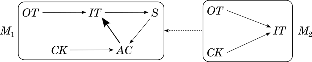
Let us now see how the static problem can be solved for our exemplary mechanism within the modified MLCM approach. The static problem concerns our exemplary mechanism when it has reached equilibrium. The system can be represented by the two-stage MLCM depicted in figure 2. Model M 2 represents the system at the top level. Variables OT and CK are directly causally relevant to IT. Model M 1 provides more detailed information about what is happening within the mechanism: the inside temperature is measured by a temperature sensor (S), which is directly causally relevant to an air conditioner (AC), which, in turn, is under direct causal influence of CK.
Figure 2.

Model M 1 is assumed to satisfy the d-connection condition, and M 2 is a restriction of M 1. The MLCM mechanistically explains why OT is relatively insensitive to IT when the cycle  has reached equilibrium and CK = on, that is, why
 holds. If CK is off, then AC is off, and there is no self-regulation due to the causal cycle
 . Thus, OT will have an influence on IT. But when CK is set to one of its on values, then AC responds to S according to CK’s adjustment. Since AC → IT overwrites OT → IT when CK = on, IT’s value is robust with respect to changes of OT’s value when CK = on. This overwriting property of AC → IT is represented by the bold arrow in figure 2.
Let us finally mention some open problems. First, cyclic models possibly featuring bidirected arrows do not admit the Markov factorization. Since we assume the d-connection condition to hold, they do, however, factor according to the following equation:

The set dSep(Xi) is constructed as follows: Let Pred(Xi) be the set of Xi’s predecessors in the ordering  . Now search for sets
 such that
 d-separates Xi from all elements of dPred(Xi). (Note that U may be empty.) If there are no such sets dPred(Xi), then identify dSep(Xi) with Xi’s predecessors Pred(Xi). If there are such sets dPred(Xi), then take one of the largest of these sets and identify dSep(Xi) with the corresponding separator set
 . For the ordering P(OT, CK, IT, AC, S), for example, the joint distribution of M 1 factors as
 .
Equation (2) has two disadvantages. First, it depends on an ordering of variables. Second, a probability distribution that factors according to equation (2) may not imply all independencies implied by the d-connection condition. For example, it does not imply an independence between OT and S conditional on {IT, AC}, although OT and S are d-separated by {IT, AC}. One open problem is to find out whether there is an order-independent factorization criterion equivalent with the d-connection condition. Another open problem is search. Causal discovery of the latent structure inside a mechanism’s causal arrows in the possible presence of feedback loops can be expected to be an even harder problem than discovery without feedback (cf. Murray-Watters and Glymour Reference Murray-Watters and Glymour2015).
We conjecture that effects of interventions for cyclic graphs possibly featuring bidirected arrows can be computed as usual. To compute postintervention probabilities  for an instantiation z of a set of variables Z, one needs, first, to delete all the arrows with an arrowhead pointing at X from the graph.Footnote 7 Second, use d-separation information provided by the manipulated graph to compute
 .
Before we take a look at how to solve the dynamic problem, let us briefly discuss the relationship of the solution to the static problem suggested above with Clarke et al.’s (Reference Clarke, Leuridan and Williamson2014) solution. Although both approaches use Pearl’s (Reference Pearl2000) notion of d-separation instead of CMC to account for cycles, the structures used for probabilistic reasoning differ in the two approaches. Clarke et al. use the “true” cyclic graph to construct an equilibrium network, that is, a BN that is then used “to model the probability distribution of the equilibrium solution” (Reference Clarke, Leuridan and Williamson2014, sec. 6.1). In our view, this move has at least two shortcomings:
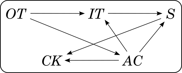
i) Independencies implied by the d-connection condition and the original cyclic causal structure may not be implied by the equilibrium network. We illustrate this by means of our model M 1, whose equilibrium network could be the one depicted in figure 3. (See Clarke et al. [Reference Clarke, Leuridan and Williamson2014], sec. 6.1, for details on how to construct equilibrium networks.) Now note that OT and CK, for example, are not d-separated in the equilibrium network. So the equilibrium network’s graph does not capture the independence between OT and CK implied by the d-connection condition and the fact that OT and CK are d-separated in M 1’s graph.
ii) Since the arrows of the equilibrium network do not capture the “true” causal relations anymore, it cannot be used for predicting the effects of interventions. To illustrate this, assume we are interested in the postintervention probability
 in our model M 1. In case we use M 1’s graph for computing this probability, we arrive at . If we use the equilibrium network’s graph, however, we arrive at . But since the control knob is causally relevant for the sensor, P(s|ck) will not equal P(s) when intervening on CK.


Figure 3.

4.2. Solving the Dynamic Problem
Solving the dynamic problem requires an extension of the MLCM approach that allows for representing the system’s behavior over a period of time. Clarke et al. (Reference Clarke, Leuridan and Williamson2014) model such behavior by means of DBNs (cf. Murphy Reference Murphy2002). The basic idea behind this move is to roll out the causal cycles over time. We use dynamic causal models (DCMs) that also allow for bidirected arrows.
A DCM M is a quadruple  , where V is a set of infinitely many variables
 . The variables X i,1 (with 1 ≤ i ≤ n) describe the system at its initial state (stage 1), the variables X i,t+1 (with 1 ≤ i ≤ n), the system at later stages t + 1. The DCMs we consider involve some idealization: directed arrows only connect variables at different stages, and if there is a directed arrow going from a variable X i,t to a variable X j,t+u for some stage t, then for every stage t there is such a directed arrow going from X i,t to X j,t+u. So the pattern of directed arrows between stages t and t + u is always the same.
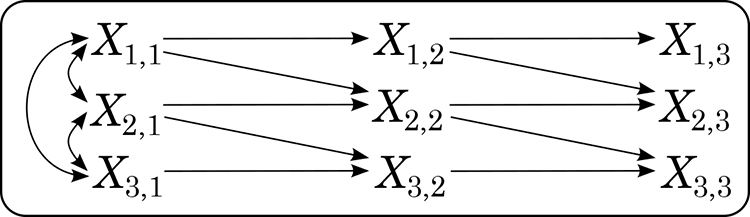
What one ideally wants is a DCM 〈V, E, P, t〉 with the following additional properties: (i) arrows do not skip stages, (ii) bidirected arrows occur only between variables of one and the same stage, (iii) every two stages ti, tj (with i, j > 1) share the same pattern of bidirected arrows, and (iv)  holds for all X i,t ∈ V with t > 1. For a finite segment of such an “ideal” DCM, see figure 4. The depicted graph’s first stage features more bidirected arrows than later stages. These additional bidirected arrows account for correlations between X 1,1 and X 2,1, X 2,1 and X 3,1, and X 1,1 and X 3,1 because of not-represented past common causes (of the kind described by variables in V).
Figure 4.

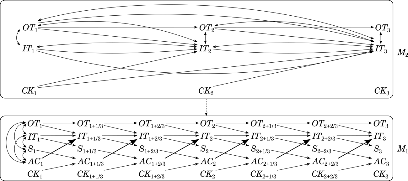
Let us now come back to the question of how the dynamic problem can be solved within the MLCM approach. The phenomenon we are interested in is that IT is relatively robust to variations of OT over a period of time when CK = on. Our simple temperature regulation system can be modeled by a two-stage MLCM 〈M 1, M 2〉 (see fig. 5 for a finite segment). The mechanism’s top level is represented by M 2, which is a restriction of M 1. Model M 1, which is assumed to satisfy the d-connection condition, provides more detailed information about the mechanism bringing about the phenomenon of interest.
Figure 5.

When adding new intermediate causes, we will typically also add new stages. In our example, we added two new variables (S and AC) and two new stages between consecutive stages of M 2 arriving at  in M 1. We assume the intervals between M 1’s stages to correspond to the time the causal processes we are interested in require to bring about their effects. To guarantee that M 1’s and M 2’s probability distributions fit together, we require t* = t,
 ,
 ,
 , and so on (where t stands for M 2’s and t* for M 1’s stages).
Now M 1 provides information about the causal structure within the temperature regulation system. Variables OT and IT are directly causally relevant to themselves at the next stage. Variable IT also causally depends on OT and AC, while S depends only on IT, AC only on S and CK, and CK on no variable in the model. The bidirected arrows at stage 1 account for dependencies to be expected because of not-represented common causes.
Here we assumed that model M 1 is especially nice, that is, that it satisfies (i)–(iv) discussed a few paragraphs above. Unfortunately, model M 2 is not that nice. Since we marginalized out S and AC and there were directed paths from  to
 and from
 to
 all going through
 or
 in M 1, M 2 features directed arrows
 and
 skipping stages. Since there were paths indicating a common cause path between
 and
 going through
 or
 in M 1, M 2 features bidirected arrows
 . Note that there are also bidirected arrows between OT t and IT t+1 and between IT t and IT t+1.
Now the MLCM mechanistically explains why IT is relatively robust with respect to OT changes when CK = on over a period of time. If CK is off over several stages, then also AC is off, and there is no regulation of IT over paths  ; IT’s value will increase and decrease (with a slight time lag) with OT’s value. If, however, CK is fixed to one of its on values over several stages, then over several stages
 responds to
 according to
 ’s adjustment. Now the crucial control mechanism consists of
 and its parents
 ,
 , and
 . The bold arrows
 in figure 5 overwrite
 and
 when
 ; that is,
 holds, where
 . This control mechanism will, after a short period of time, cancel deviations of IT’s value from CK’s adjustment brought about by OT’s influence.
Here are some possible open problems: first, some of the arrows in M 2 may seem to misrepresent the “true” causal processes going on inside the temperature regulation system. There is, for example, a directed arrow going from CK t to IT t+1 but no directed arrow from CK t to AC t+1, although CK can clearly influence IT only through AC. This is a typical problem arising for dynamic models. One can, however, learn something about M 1’s structure from M 2: the (direct or indirect) cause-effect relationships among variables in M 2 will also hold for M 1. Another problem is, again, search. For solutions of several discovery problems involving time series, see, for example, Danks and Plis (Reference Danks and Plis2014). Finally, factorization and interventions: since our DCMs do not feature feedback loops, we conjecture that Richardson’s (Reference Richardson, Bilmes and Ng2009) factorization criterion and Zhang’s (Reference Zhang2008) results about how to compute the effects of interventions in models with bidirected arrows can be fruitfully applied to DCMs.
Let us finally have a look at how our solution to the dynamic problem relates to the one suggested by Clarke et al. (Reference Clarke, Leuridan and Williamson2014). Both modeling strategies use the same basic idea, that is, to roll out the cycles over time. While the arrows of the DCMs we use are intended to capture the “true” causal relations between variables of interest, the directed arrows in Clarke et al.’s DBNs surprisingly are not intended to represent the “true” causal relationships (cf. sec. 6.2). Thus, their models share problem (ii) discussed at the end of section 4.1 with the equilibrium network they use for solving static problems: the model cannot be used to compute the effects of interventions.
5. Conclusion
Clarke et al. (Reference Clarke, Leuridan and Williamson2014) have extended Casini et al.’s (Reference Casini, lllari, Russo and Williamson2011) RBN approach for modeling mechanisms in such a way that it can be applied to mechanisms featuring causal feedback. In this article we followed their example and showed how the MLCM approach can be modified in a similar way. Like Clarke et al. we distinguish between static and dynamic problems when it comes to modeling mechanisms with causal cycles. Our solutions to both problems within the MLCM approach mirror Clarke et al.’s solutions for the RBN approach while avoiding several problems. The MLCM approach can be used for modeling mechanisms whose causal cycles have reached equilibrium (i.e., static problems) by introducing the requirement that the most detailed causal model M 1 has to satisfy the d-connection condition instead of CMC. The dynamic problem, which concerns the development of the system over a period of time, can be solved within the MLCM approach by using DCMs. Both solutions, however, come with new challenges, whose investigation we leave to future research.