


1. Introduction
Civil wars rarely unfold as simple contests between governments and unified rebel organizations. Contemporary conflicts feature multiple armed actors whose fighting relationships shift through fragmentation, realignment, and strategic adaptation (Bakke et al., Reference Bakke, Cunningham and Seymour2012; Cunningham et al., Reference Cunningham, Bakke, Seymour, Pearlman and Cunningham2012; Metternich et al., Reference Metternich, Dorff, Gallop, Weschle and Ward2013). State forces battle competing rebel factions while those same rebels fight each other for resources and legitimacy. Pro-government militias switch sides when the opportunity arises. Foreign forces intervene, further complicating the conflict environment. These constantly shifting patterns of violence raise a question for the intrastate conflict literature, when do negotiations become possible in such a fluid, multi-actor environment?
Two influential theoretical traditions bear on this question, and they appear to make opposite predictions about the role of stability. Bargaining accounts ask what prevents parties who want to settle from reaching agreement; the answer centers on information asymmetries and commitment problems (Fearon, Reference Fearon1995; Powell, Reference Powell2002). In this framework, stable conflict environments should facilitate negotiation: consistent patterns of violence reveal relative capabilities, clarify organizational boundaries and command structures, and make it easier to identify legitimate negotiating partners and assess whether agreements can be implemented (Cunningham, Reference Cunningham2013; Staniland, Reference Staniland2014; Walter, Reference Walter1997). Yet, a bargaining-based account explains why legibility and commitment capacity matter for talks, but it does not by itself specify when actors will choose to incur the costs of opening negotiations. Actors who have adapted to a predictable conflict environment may prefer continuation over the risks of settlement.
Ripeness accounts ask a different question: what prevents parties who could settle from wanting to Zartman (Reference Zartman1985, Reference Zartman, Stern and Druckman2000)? The answer has two components. First, parties need both a mutually hurting stalemate that makes continuation intolerable and, second, a perceived “way out” that makes settlement conceivable. From this perspective, disruption—a shock that invalidates actors’ existing expectations about who they are fighting, within what coalitional structure, and at what intensity—creates openings for bargaining by breaking entrenched equilibria and imposing costs. Yet, ripeness accounts leave open how parties navigate the uncertainty that disruption creates. If the conflict environment is in flux, identifying partners and assessing commitments becomes harder, which is precisely the problem bargaining theory highlights. The two traditions have largely developed in parallel rather than in direct engagement, and their apparently contradictory predictions about stability have not been systematically addressed.
We propose that these traditions describe different phases of a single process and that the apparent contradiction dissolves when they are sequenced. Our core insight is that bargaining theory’s stability requirement and ripeness theory’s disruption requirement are not competing conditions for the same moment but sequential prerequisites: disruption comes first, followed restabilization.
By disruption we mean a deterioration shock to the conflict network—a period in which established fighting relationships break down, new actors enter or old ones fragment, and the dyadic structure that actors had adapted to becomes unreliable. Such shocks operate through the ripeness mechanism; they break entrenched equilibria, lower continuation payoffs, and create pressure to reconsider strategies. But disruption alone does not produce negotiations, because the same instability that motivates talks also undermines the conditions for initiating them—if no one knows who the relevant bargaining partners are, talks cannot begin.
Recovery opens the window for negotiation. Recovery is the subsequent period following a disruption in which the conflict network reconsolidates into a new legible configuration. Crucially, this is not a return to the old equilibrium. It is a new configuration in which salient dyads and coalitional alignments have clarified, but actors have not yet had time to entrench into these positions. This is what distinguishes post-disruption recovery from undisrupted stability: both are legible, but only recovery coexists with the increased willingness to fight that disruption creates. In an undisrupted stable conflict, actors can read the landscape but have optimized for continued fighting; in a post-disruption recovery, actors can read the new landscape but have renewed the motivation to consider alternatives. That temporary configuration—legibility without entrenchment—is where negotiations begin, and it closes as actors adapt to the new status quo.
We test our logic using temporal network analysis of conflict dynamics across 21 African countries (1999–2013). Using ACLED battle events, we construct semiannual conflict networks in which nodes represent armed actors (government forces, rebel groups, and militias) and edges capture combat relationships weighted by battle frequency. Our durability measure combines edge persistence (whether the same groups continue battling each other) and intensity correlation (whether actors’ relative conflict involvement remains stable across periods) (Christia, Reference Christia2012; Metternich et al., Reference Metternich, Dorff, Gallop, Weschle and Ward2013). We operationalize the two stages using semiannual durability values within a window specification: prior disruption (within-year network destabilization during year
 $t{-}2$
) and subsequent recovery (cross-year network improvement from
 $t{-}2$
to
 $t{-}1$
).
Our analysis shows that the window configuration—prior disruption followed by recovery—is a significant predictor of negotiation onset. Country-years in the window configuration have substantially higher onset rates than the baseline, and more than half of observed onsets occur in this configuration despite it comprising about a fifth of observations.Footnote 1 Semiannual measurement of network dynamics captures within-year disruption-recovery sequences that annual network measures would smooth over Bakke et al. (Reference Bakke, Cunningham and Seymour2012; Tamm, Reference Tamm2016).
Three patterns emerge. First, negotiation onsets cluster in the window configuration. Negotiations tend to begin not at peak turbulence but as networks reconsolidate after disruption. Second, while network dynamics predict negotiation onset, they show no association with peace agreement conclusion, suggesting the factors that initially bring parties to the table differ from those that enable full agreements. Third, following negotiation onset, networks reorganize. Some cases fragment while others consolidate, indicating that talks can coincide with case-specific reorganization rather than a uniform trajectory.
These findings support the sequencing argument. Neither prior disruption nor recovery alone is significant, but onsets concentrate in the window where both co-occur. The two-stage framework captures both the pressure emphasized by ripeness theory and the feasibility emphasized by bargaining theory, and the key distinction it draws is between post-disruption recovery and undisrupted stability. Both are legible, but only recovery coexists with an increased willingness to fight that disruption creates. That temporary configuration, legibility without entrenchment, is where negotiations begin.
2. Theory
2.1 Network dynamics and negotiation timing
Civil wars are increasingly multi-actor conflict systems rather than simple state–rebel dyads. Armed actors enter, split, align, and redirect violence, and these shifts can reshape bargaining conditions (Cunningham et al., Reference Cunningham, Bakke, Seymour, Pearlman and Cunningham2012; Dorff et al., Reference Dorff, Gallop and Minhas2020; Metternich et al., Reference Metternich, Dorff, Gallop, Weschle and Ward2013). Network approaches capture these interdependencies: when one dyad changes, other actors update strategies in response to shifting coalitional balance and local rivalries (Bakke et al., Reference Bakke, Cunningham and Seymour2012; Rudloff and Findley, Reference Rudloff and Findley2016).
A growing literature examines the conditions under which negotiations begin, linking onset to military stalemates, third-party intervention, rebel organizational characteristics, disasters, and the strategic calculations of internally divided movements (Cunningham, Reference Cunningham2011; Kaplow, Reference Kaplow2016; Rosvold and Rustad, Reference Rosvold and Rustad2026). Peace-process scholarship also shows that conflict resolution unfolds across three distinct stages: entering talks, reaching agreement, and implementing terms. The correlates of each can differ. Walter (Reference Walter2002); Findley (Reference Findley2013). Research on fragmentation shows that internal divisions can intensify commitment and information problems, but fragmentation does not uniformly prolong war or preclude negotiated outcomes (Bakke et al., Reference Bakke, Cunningham and Seymour2012; Cunningham, Reference Cunningham2013). Yet, this work has largely focused on dyadic or actor-level predictors rather than system-wide network reorganization. Our contribution is to identify a network-level micro-sequence within the transition to talks: not whether fragmentation helps or hurts, but when and how the timing and sequence of network reorganization create a window for onset.
Despite advances in mapping conflict networks, we lack systematic evidence on how changes in network structure shape the timing of negotiation onset. Bargaining and ripeness traditions offer apparently opposing predictions. Bargaining theory starts from the puzzle that mutually preferable bargains should often exist, yet actors still fail to reach them; in civil war, the core barriers are private information and credible-commitment problems (Fearon, Reference Fearon1995; Walter, Reference Walter1997). In a multi-actor extension of that logic, more legible and organizationally coherent conflict environments should reduce barriers to negotiation by clarifying who can commit and who can implement, though bargaining logic alone does not specify when actors will choose to incur the costs of opening talks (Kaplow, Reference Kaplow2016). Ripeness theory addresses timing directly: serious negotiations become likely when parties perceive both a mutually hurting stalemate and a “way out” (Zartman, Reference Zartman1985, Reference Zartman, Stern and Druckman2000). Our network measures are not direct observations of those perceptions but observable proxies for conditions likely to shift actors’ assessments of stalemate and feasibility in multi-actor settings.
These approaches ask fundamentally different questions. Bargaining asks what prevents settlement given willingness; ripeness asks what prevents willingness given the ability to settle. We argue below that sequencing the two logics resolves the apparent contradiction. Disruption generates the pressure side of ripeness (creating motivation), while recovery provides the network form of a way out by restoring the legibility that bargaining logic identifies as necessary.
We conceptualize durability as the extent to which dyadic conflict structure persists over time. High durability means that the set of fighting dyads is similar across periods and that actors’ relative conflict involvement is broadly consistent. Low durability indicates turnover in who fights whom and changes in relative engagement. Importantly, instability can reflect two distinct features: a low level of durability (a system that is persistently fluid) and a trajectory of change (a system that is deteriorating or recovering). A conflict can be chronically low in durability yet improving or relatively durable yet deteriorating. We therefore distinguish durability level from durability trajectory and test whether negotiation onset is more closely associated with the state of the conflict system or its direction of movement.
2.2 Pressure: How deterioration shocks create incentives
We outline two complementary forces that shape negotiation timing in multi-actor conflicts: pressure from deterioration shocks and feasibility from subsequent recovery. The framework is probabilistic since it identifies conditions under which onset is more likely, not conditions that make onset inevitable.
Durable conflict networks support entrenched patterns of violence. When dyadic structure is predictable, actors can adapt militarily and organizationally, develop routines, and pursue strategies calibrated to a known environment (Kalyvas, Reference Kalyvas2006; Wood, Reference Wood2003). Over time, these routines can sustain continued fighting even when peace would be preferable in the abstract. Entrenchment is not an information problem (actors in stable conflicts may have clear information about capabilities and partners) but a reservation-value problem. In other words, continuation payoffs in the known environment exceed expected payoffs from uncertain negotiations, so nobody comes to the table.
A key implication is that incentives to reconsider strategies may arise less from chronic disorder than from deterioration shocks that invalidate recent expectations. This is the logic that ripeness accounts identify: disruption breaks the sustainability of the status quo, lowers continuation payoffs, and makes actors more willing to consider alternatives (Zartman, Reference Zartman1985, Reference Zartman, Stern and Druckman2000). When durability declines relative to the recent past, actors face sharper reassessment problems. Coalition partners are less reliable, recent bargaining expectations become harder to extrapolate, and the set of active opponents may shift quickly. These shifts increase uncertainty about future outcomes and weaken confidence in battlefield victory, widening the perceived space for bargaining (Fearon, Reference Fearon1995; Powell, Reference Powell2004). They can also impose distributed costs across multiple actors when realignments and rivalries intensify, creating conditions that resemble the mutually hurting stalemates emphasized in the ripeness literature. The mechanism is not chronic disorder but a shock relative to the recent past. More precisely, deterioration shocks capture the pressure component of ripeness rather than ripeness in full; they can make continuation less attractive without yet establishing that actors perceive a feasible exit. In our empirical tests, we operationalize pressure as a decline in durability into
 $t{-}2$
relative to
 $t{-}3$
(
 $D_{t-2} \lt D_{t-3}$
).
2.3 Feasibility: How recovery restores legibility
Pressure alone is not sufficient. Ripeness theory itself recognizes this. Zartman (Reference Zartman1985) requires not only a mutually hurting stalemate but also a perceived “way out,” a sense that a negotiated settlement is feasible. Bargaining accounts formalize that feasibility requires legibility and organizational capacity (Fearon, Reference Fearon1995; Walter, Reference Walter1997). When dyadic structure is more stable, parties can form clearer assessments of who matters, who can implement, and what kinds of guarantees might be necessary (Cunningham, Reference Cunningham2013; Staniland, Reference Staniland2014). In multi-actor settings, feasibility is not only about relative power; it is also about whether bargaining partners can be identified and whether commitments can plausibly be delivered by the relevant organizations and coalitions. The environment also shapes incentives for brief cessation of fighting. Disasters can create opportunities for ceasefires where rebels want to regroup or gain public support (Rosvold and Rustad, Reference Rosvold and Rustad2026). If disruption alone were sufficient, we would expect chaotic conflicts to produce negotiations, but they often do not, precisely because the uncertainty that motivates talks also undermines the conditions for initiating them.
We propose that a network’s trajectory informs feasibility. A recovering network (improving durability) suggests that a period of restructuring is ending and that dyadic conflict structure is becoming more legible. Even if the system remains far from fully stable, improvement can signal consolidation and provide a clear enough set of salient dyads and coalitional alignments for negotiations to begin.
The crucial distinction is between post-disruption recovery and undisrupted stability. An undisrupted stable conflict has legibility but also entrenchment. Actors can read the landscape but have optimized for it, and their continuation payoffs exceed their negotiation payoffs. A post-disruption recovery has legibility without entrenchment. Actors can read the new landscape (salient dyads and coalitional alignments have clarified) but have not yet had time to dig in and optimize for continued fighting. This provides the clarity that bargaining theory identifies as necessary for talks to work, alongside the motivation that ripeness theory identifies as necessary for talks to start. The window exists because legibility and motivation rarely co-occur. Stable systems have legibility but not motivation, chaotic systems have motivation but not legibility, and post-disruption recovery is the configuration where both are present. It is also temporary, because actors re-entrench as the new configuration stabilizes. We operationalize feasibility as a rebound in durability into
 $t{-}1$
relative to
 $t{-}2$
(
 $D_{t-1} \gt D_{t-2}$
).
2.4 The window of opportunity
The window of opportunity hypothesis combines these stages. Pressure without feasibility describes periods in which durability has declined but continues to deteriorate; costs may be rising, but partner identification and credible commitment are less clear. Feasibility without pressure describes periods in which durability is improving without a preceding deterioration shock; bargaining conditions may be clearer, but incentives to initiate talks may be weaker. This is the entrenchment problem in a different guise, as recovery without prior disruption resembles ordinary stability.
The window is the sequence in which prior disruption is followed by recovery. In this configuration, a deterioration shock creates the motivation that ripeness accounts identify as necessary (the pressure stage), and subsequent recovery creates the legibility that bargaining accounts identify as necessary (the feasibility stage). A pure legibility account would predict that recovery should help regardless of prior disruption; a pure pressure account would predict that disruption should matter even absent recovery. Classic ripeness is closer to our full argument because it already requires a perceived way out, but it does not specify what that way out looks like in network terms. Our framework specifies the network-level content of that way out: recovery is the moment when salient dyads, coalition structure, and likely implementers become legible enough for actors to treat negotiation as a viable exit rather than a leap into organizational uncertainty. The sequencing framework thus predicts that recovery matters only following disruption and that disruption is most consequential when followed by recovery. Negotiations should be concentrated in this configuration, though onset remains possible in other configurations. Figure 1 displays the window of opportunity framework.
Window-of-opportunity framework. The framework distinguishes prior disruption (
 $D_{t-2} \lt D_{t-3}$
) and subsequent recovery (
 $D_{t-1} \gt D_{t-2}$
). The window is the configuration in which disruption is followed by recovery. The framework is probabilistic since onset is expected to be more likely in the window configuration than in the other quadrants.

2.5 Illustrative cases
We illustrate these patterns with three conflicts in Africa. Two cases fall into the window of opportunity framework (Mali 2012 and CAR 2011), and one shows an exception falling outside the window quadrant (Sudan 2012). Of the 9 negotiation onsets in the estimation sample, 5 (55.6%) occur in the window configuration (prior disruption followed by recovery) while 4 occur in other quadrants. Figure 2 displays two window cases and one exception.
Durability trajectories preceding negotiation onset. Panel A: CAR (2011) illustrates the window pattern with within-year disruption in 2009 followed by cross-year recovery into 2010. Panel B: Mali (2012) illustrates another window pathway with within-year disruption in 2010 followed by cross-year recovery into 2011. Panel C: Sudan (2012) illustrates a case falling in the “neither” quadrant under the window framework. Dashed vertical line indicates negotiation onset.

Mali 2012. Mali’s conflict landscape underwent dramatic transformation in the years preceding negotiation onset (Lecocq et al., Reference Lecocq, Mann, Whitehouse, Badi, Pelckmans, Belalimat, Hall and Lacher2013; Wing, Reference Wing2013). Northern Mali had experienced recurring Tuareg insurgencies since independence (Lecocq and Klute, Reference Lecocq and Klute2013), but the conflict network restructured significantly within 2010 as AQIM (Al-Qaeda in the Islamic Maghreb) consolidated its presence in the north – conducting kidnappings and provoking government and international military responses that altered existing fighting configurations. Within-year network stability collapsed (
 $D$
fell from 0.509 to 0.180), reflecting this restructuring of conflict relationships across the northern theater.
By the cross-year transition into 2011, the network had reconsolidated (
 $D$
recovered to 0.564) as conflict relationships clarified into more stable configurations. The window pattern is visible: disruption within 2010 created pressure as the old equilibrium broke, and recovery crossing into 2011 provided feasibility as the conflict landscape became newly legible. The situation then escalated sharply. As Libya collapsed into civil war in 2011, heavily armed Tuareg fighters returned to Mali, a process that accelerated after Gaddafi’s fall in October (Lecocq and Klute, Reference Lecocq and Klute2013). The MNLA (National Movement for the Liberation of Azawad) launched a coordinated offensive in January 2012, quickly overrunning government positions. Islamist groups – Ansar Dine, AQIM, and MUJAO (Movement for Oneness and Jihad in West Africa) – cooperated with the MNLA in seizing northern cities but pursued distinct objectives, and by mid-2012 Ansar Dine controlled Kidal and Timbuktu while MUJAO held Gao (Lecocq et al., Reference Lecocq, Mann, Whitehouse, Badi, Pelckmans, Belalimat, Hall and Lacher2013; Wing, Reference Wing2013). Following the March 2012 military coup in Bamako and the MNLA’s declaration of Azawad independence in April, ECOWAS appointed a mediator, and negotiations began in 2012.
Central African Republic 2011. The CAR conflict had reached a violent equilibrium following the 2007 Birao peace agreement. The government of François Bozizé controlled Bangui and major towns while three main rebel coalitions held distinct territories in the north. The Union of Democratic Forces for Unity (UFDR) maintained strongholds in the Vakaga prefecture in the far northeast near the Sudanese border. The Convention of Patriots for Justice and Peace (CPJP), based around Ndele, contested diamond mining areas in the north-central and eastern prefectures. The People’s Army for the Restoration of Democracy (APRD) operated in the northwest (Lombard, Reference Lombard2016; Mehler, Reference Mehler2011). This configuration produced persistent violence that all parties had adapted to survive.
The network disrupted dramatically within 2009. The CPJP, formed in late 2008 by ethnic Runga fighters in opposition to the Goula-led UFDR, escalated its challenge to both the government and rival rebel groups over control of diamond mining areas around Sam Ouandja and Ndele (Spittaels and Hilgert, Reference Spittaels and Hilgert2009). New self-defense militias emerged in response to increased banditry as the security situation deteriorated. Armed groups clashed in new configurations as they competed for control of mining sites and trade routes (
 $D$
fell from 0.466 to 0.131). The government, facing proliferating threats on multiple fronts, could no longer maintain its strategy of containing rebels to peripheral zones (Agger, Reference Agger2015). The window pattern is visible in the durability trajectory: within-year stability collapsed as the network restructured, creating a deterioration shock that increased pressure.
By the cross-year transition into 2010, durability rebounded (
 $D$
recovered to 0.576) as the network began to consolidate. The within-year disruption operated through the ripeness logic: fragmentation made existing strategies untenable for both the government and rebel leaders, who recognized that continued splintering was eroding their political leverage and military (International Criminal Court, Office of the Prosecutor, 2014). The cross-year recovery operated through the bargaining logic: as the network began to consolidate, the military situation clarified enough to identify who could negotiate and what commitments were feasible, but the new configuration was too recent for actors to have re-entrenched into it. The window opened, and the CPJP entered negotiations and eventually signed a ceasefire in June 2011 (Reuters, 2011; United Nations Secretary-General, 2009).
Sudan 2012. Following South Sudan’s independence in July 2011, the Sudanese government faced insurgencies across multiple fronts: escalating fighting in Darfur and new conflicts in South Kordofan (from June 2011) and Blue Nile (from September 2011) (International Crisis Group, 2013). In November 2011, four rebel groups – the Justice and Equality Movement (JEM), two Sudan Liberation Movement/Army factions (SLM-Abdel Wahid and SLM-Minnawi), and SPLM-North – formed the Sudan Revolutionary Front (SRF), a coalition that sought to coordinate opposition across these theaters (Gramizzi and Tubiana, Reference Gramizzi and Tubiana2013). Despite the SRF’s aspiration to negotiate as a unified bloc, the government pursued bilateral channels. Talks with a JEM splinter faction began in Doha in late 2012, and the AU High-Level Implementation Panel brokered direct negotiations between the government and SPLM-North beginning in 2013 (Knopf, Reference Knopf2011; Permanent Mission of South Sudan to the United Nations, 2012). Under the window framework, Sudan falls in the “neither” quadrant because the network did not exhibit the within-year disruption followed by cross-year recovery that characterizes the window. This exception suggests that onset can occur outside the window configuration. Here, the political dynamics surrounding the SRF’s formation and the post-independence crises created pressure for talks through channels that our network recovery measure does not capture (Zartman, Reference Zartman1985). Sudan thus clarifies a scope condition: the window framework describes the typical path, but alternative sources of pressure and feasibility can operate through political rather than network-structural mechanisms.
Across the window cases, the common thread is not disruption or recovery alone but the sequence: pressure first, then legibility, then talks. The Sudan exception shows that alternative pathways exist, but the window cases illustrate the typical pattern. Semiannual measurement of network dynamics is important for capturing these sequences, since the within-year disruption-recovery patterns unfolded over months, not years, and annual network measures would have smoothed over the window dynamics that preceded negotiations (Tamm, Reference Tamm2016).
2.6 Hypotheses
The sequencing framework generates specific predictions about each stage and their combination. If disruption creates motivation through the ripeness mechanism and recovery creates legibility through the bargaining mechanism, then the strongest signal should come from the sequence in which both operate. This implies a two-stage pattern in durability changes prior to onset: (i) a decline in durability into
 $t{-}2$
(pressure), followed by (ii) an improvement into
 $t{-}1$
(feasibility), both observed before onset at
 $t$
.
H1 (Window sequence): Negotiation onset is more likely when a durability decline into
 $t{-}2$
(
 $D_{t-2}\lt D_{t-3}$
) is followed by a durability rebound into
 $t{-}1$
(
 $D_{t-1}\gt D_{t-2}$
).
The constituent stages yield further predictions that distinguish the sequencing framework from either tradition alone:
H1a (Pressure stage): A durability decline into
 $t{-}2$
is associated with a higher hazard of onset. This captures the pressure component of the ripeness logic. Disruption creates motivation by breaking entrenched equilibria and lowering continuation payoffs.
H1b (Feasibility stage): Conditional on prior decline, a durability rebound into
 $t{-}1$
is associated with a higher hazard of onset. Importantly, recovery without prior disruption should not predict onset on its own, because recovery in the absence of a preceding shock resembles ordinary stability, that is, legibility without motivation. This distinguishes the sequencing framework from a pure bargaining account, which would predict that recovery helps regardless of prior disruption.
Our second hypothesis addresses whether the same network dynamics that facilitate negotiation onset also promote peace agreement conclusion. The sequencing framework predicts an asymmetry; the factors that create the window (pressure from disruption, feasibility from recovery) are about getting parties to the table, not about what happens once they are there. Agreement conclusion depends on a different set of factors: bargaining dynamics during negotiations, third-party guarantees, and agreement design and implementation credibility that network-level measures do not capture (Mattes and Savun, Reference Mattes and Savun2009; Walter, Reference Walter2002). Fragmented networks can create commitment problems as parties cannot credibly promise to control all armed actors within their nominal coalitions (Cunningham, Reference Cunningham2006). Thus, we anticipate a null relationship between network dynamics and agreement conclusion despite effects on negotiation onset. The onset–agreement asymmetry is itself a prediction of the sequencing theory, not merely an empirical surprise.
H2 (Agreements): Network dynamics do not show a detectable association with peace agreement conclusion.
Our third hypothesis examines how networks evolve after negotiations begin. We expect that networks undergo reorganization following negotiation onset, though the direction is theoretically ambiguous. Several processes drive post-onset change. The announcement of negotiations often triggers defections as hardline elements reject talks and form splinter groups (Kydd and Walter, Reference Kydd and Walter2002). Excluded actors may escalate violence to gain seats at the negotiating table or spoil processes that threaten their interests (Nilsson, Reference Nilsson2008; Stedman, Reference Stedman1997). The reduction in violence between negotiating parties can create security vacuums that new armed groups exploit. Yet, consolidation is also possible as weaker actors align with stronger ones or exit the conflict entirely.
H3 (Reorganization): Negotiation onset is associated with network reorganization, with direction and magnitude varying across cases.
The asymmetry between these hypotheses reflects a tension in peace processes. The conditions that make conflicts ripe for negotiation may simultaneously make them difficult to resolve. Recovery creates feasibility for talks, but the underlying instability that created pressure may reassert itself through post-onset reorganization. This distinction suggests that models of negotiation onset and agreement conclusion may require different explanatory variables.
3. Research design
3.1 Data
We analyze civil conflicts from 1999 to 2013 using semiannual temporal resolution. Our primary data come from the Armed Conflict Location and Event Data (ACLED) project, which provides georeferenced information on political violence events (Raleigh et al., Reference Raleigh, Linke, Hegre and Karlsen2010). From ACLED, we extract battle events that form the basis of our network construction. These battles represent direct combat interactions between armed actors, excluding one-sided violence against civilians and remote violence. ACLED identifies actors by organizational name and codes battle events between specific pairs, enabling network construction. Our analysis draws on ACLED’s Africa coverage, which is the most comprehensive and temporally consistent during our study period; our analysis window begins in 1999 to allow lag construction.
Negotiation data come from the Peace Negotiations in Civil Conflicts (PNCC) dataset, which systematically codes formal bilateral talks between governments and rebel groups (Arı, Reference Arı2022). PNCC codes negotiations at the dyad-year level, recording whether a government–rebel dyad was in the formal negotiation phase in each year. We use this annual coding directly as our outcome measure. Negotiation onset is coded as the first year in which any government–rebel dyad enters negotiations after a period with no active negotiations in that country; continuing negotiations in subsequent years are excluded from the risk set to ensure proper hazard-model interpretation. Countries can experience multiple onsets if negotiations lapse and later resume.
To examine whether network dynamics affect not just negotiation onset but also successful resolution, we incorporate peace agreement data from the PA-X Peace Agreement Database (Bell and Badanjak, Reference Bell and Badanjak2019). PA-X defines agreements as “formal, publicly-available documents, produced after discussion with conflict protagonists and addressing conflict with a commitment to peace.” This includes ceasefires, framework agreements, comprehensive settlements, and implementation protocols, a heterogeneous set capturing the full peace process. This dataset identifies 30 agreement events within the analysis sample used for our window specification. The higher frequency of agreements compared to negotiation onsets reflects both the inclusion of agreements reached without formal negotiations and the reality that some negotiation processes yield multiple agreements over time.
The temporal structure of our data deserves emphasis. While ACLED coverage extends beyond our study period, we restrict analysis to 1999–2013 given constraints of the other datasets. We construct networks at semiannual frequency, dividing each year into two six-month periods: a first half (January–June) and a second half (July–December). This semiannual measurement provides critical advantages. It captures within-year dynamics that annual network measures would smooth over, including the alliance shifts and group fragmentation documented in qualitative accounts (Bakke et al., Reference Bakke, Cunningham and Seymour2012; Tamm, Reference Tamm2016). The outcome, however, is modeled at the annual level, using PNCC’s native annual coding directly and avoiding the need to assign onsets to sub-annual periods. This combination – semiannual network measurement with annual outcome modeling – captures within-year disruption-recovery sequences in the predictors. We model the outcome annually because PNCC records negotiation onset by calendar year rather than by month or half-year; the annual outcome reflects this feature of the available data rather than a claim that negotiations begin on an annual rhythm.
The unit of analysis is the country-year. After applying the network thresholds and lag requirements and excluding continuation spells (ongoing negotiations), the estimation sample comprises 97 country-years drawn from 21 African countries (one multi-actor conflict system per country). The entire onset analysis therefore rests on 9 negotiation onsets among these 97 country-years. Appendix Table A2 details sample construction.
3.2 Network construction
We construct conflict networks to capture multi-actor dynamics that characterize contemporary civil wars. Unlike dyadic approaches that examine government-rebel interactions in isolation, network analysis reveals how armed groups interact within broader conflict systems (Bakke et al., Reference Bakke, Cunningham and Seymour2012; Cunningham et al., Reference Cunningham, Bakke, Seymour, Pearlman and Cunningham2012). Nodes represent armed actors in conflicts such as national armies, paramilitary forces, ethnic militias, rebel organizations, pro-government militias, and foreign interveners. Edges capture direct combat relationships through which these actors contest territorial control, compete for resources, and pursue political objectives.
Each edge between actors
 $i$
and
 $j$
is weighted by battle frequency (
 $w_{ij,t} = \sum _{e \in E_{ij,t}} 1$
), capturing conflict intensity that varies across dyads and time. A government may simultaneously engage multiple rebel groups with different intensities while those rebels fight among themselves for dominance within the opposition. These patterns matter for understanding when negotiations become possible by helping us to understand the central government’s relationship with the main rebel group exists within a broader ecosystem of violence that shapes bargaining dynamics (Johnston, Reference Johnston2014; Prorok, Reference Prorok2016).
We construct networks at semiannual frequency.Footnote 2 We focus exclusively on battle events because they capture the reciprocal violence central to bargaining theory. Battles represent contested interactions where both parties choose to engage, revealing information about capabilities and resolve that one-sided violence against civilians cannot provide. This distinction matters theoretically. While civilian victimization may signal desperation or strength, only direct combat tests relative military capacity, the core uncertainty driving bargaining failures in civil war (Fearon, Reference Fearon1995; Walter, Reference Walter2009).
The requirement of
 $|V| \geq 3$
actors and
 $|E| \geq 3$
edges ensures we analyze genuine multi-actor conflicts rather than simple bilateral confrontations. This threshold captures the complexity that distinguishes network wars from traditional insurgencies. Conflicts with government forces battling multiple rebel groups, rebels fighting each other for territorial control, or ethnically fragmented conflicts with shifting militia alliances. Country-semesters that fall below the threshold are excluded from durability calculations and thus from the estimation sample; our window specification requires valid semiannual durability values from the two years preceding each country-year observation, so a country-year enters the analysis only if the relevant preceding semesters also meet the network threshold. Countries may re-enter the sample if they cross back above the threshold after a gap. Networks meeting our threshold average 24 actors, enough to generate the fragmentation and coordination problems central to multi-party bargaining challenges (Cunningham, Reference Cunningham2006, Reference Cunningham2013).
3.3 Measuring network durability
Our durability measure operationalizes conflict system stability relevant to both bargaining and ripeness theories. High durability indicates an entrenched conflict equilibrium where actors have settled into predictable patterns of violence. Governments control urban centers while rebels hold rural territory, militias maintain ethnic enclaves, and all parties calibrate violence to sustainable levels (Kalyvas, Reference Kalyvas2006; Wood, Reference Wood2003). Low durability signals structural disruption, for example, when defections split rebel coalitions, new militias emerge to exploit power vacuums, or when external interventions alter the balance of forces.
We capture two dimensions of network change that theory identifies as consequential for negotiation dynamics. Each component reveals distinct mechanisms through which stability and change affect bargaining.
Edge persistence measures relationship turnover through the Jaccard coefficient:
 \begin{equation} J = \frac {|E_{t-2} \cap E_{t-1}|}{|E_{t-2} \cup E_{t-1}|} \end{equation}
where
 $E_t$
is the set of edges (fighting dyads) at time
 $t$
.Footnote
3
This captures whether the same pairs of actors continue fighting. In our sample, edge persistence averages 0.21; less than a quarter of fighting relationships persist across semiannual periods. This turnover reflects the realignments that reshape conflict dynamics. When former allies turn against each other or new actors redirect existing conflicts, these changes force all parties to reassess their strategic positions (Tamm, Reference Tamm2016). Such relationship changes matter because they affect who can negotiate with whom and whether coalitions can make credible commitments.
Intensity correlation tracks volatility in violence levels through the Pearson correlation of actor strengths:
 \begin{equation} \rho = \text{Cor}(s_{i,t-2}, s_{i,t-1}) \end{equation}
where
 $s_{i,t}$
represents actor
 $i$
’s total battle involvement (weighted degree) at time
 $t$
, computed over all actors present in either period (with zeros assigned to actors absent from one period). The correlation averages 0.61 in our data, indicating moderate stability in relative intensity rankings. Governments may escalate operations against one rebel group while reducing pressure on another. Militias intensify violence to claim negotiation seats. Rebels reduce attacks when resources dwindle. Such intensity shifts may theoretically signal changes in capabilities and resolve (Akcinaroglu, Reference Akcinaroglu2012; Weinstein, Reference Weinstein2007), though as we show below, structural continuity proves more consequential for negotiation timing.
Composite index:
 $D = (J + |\rho |)/2$
, bounded in
 $[0,1]$
. We use the absolute value of
 $\rho$
so that both perfectly stable and perfectly inverted intensity profiles indicate structural persistence; robustness checks using signed
 $\rho$
yield similar results (Appendix Table A11). Component disaggregation shows that neither edge persistence nor intensity correlation is individually significant for the window specification; the composite index captures the disruption-recovery signal more effectively than either component alone (Appendix Table A14). This suggests that coordinated change across both dimensions – whether the same dyads continue fighting and how consistently actors fight – jointly defines the network dynamics associated with negotiation timing. Stable relationship structures signal who the relevant bargaining partners are, enabling credible negotiation.
Semiannual measurement of network dynamics is important for detecting these patterns in our data. Alliance realignments in conflicts like the Democratic Republic of Congo or Central African Republic often unfold over months rather than years (Tamm, Reference Tamm2016). By measuring at six-month intervals, we capture within-year disruption-recovery sequences that annual network measures would smooth over. The window specification relies on comparing semiannual durability values within and across years; annual network aggregation would collapse these distinct phases into a single value, obscuring the within-year dynamics that carry the signal. Our system-wide approach captures broad network restructuring, whether arising from endogenous cascades (defections triggering realignments) or exogenous shocks (external interventions affecting multiple actors simultaneously). The durability measure reflects the outcome, network change, without distinguishing between these sources, which we acknowledge as a limitation.
3.4 Model specification
We estimate an annual discrete-time hazard model where each country-year represents a “trial” in which negotiation either begins or does not (Beck et al., Reference Beck, Katz and Tucker1998; Carter and Signorino, Reference Carter and Signorino2010). The binary outcome approach matches our theoretical focus on negotiation onset (the decision to begin talks) rather than the continuous process of negotiation itself. Countries enter the risk set in the first year they meet the network thresholds and contribute one country-year observation for each subsequent year they remain at risk of onset. A country leaves the risk set in the year an onset occurs and re-enters if negotiations later lapse, so a single country can contribute multiple spells. A country-year is dropped from the sample in any year the network falls below the multi-actor threshold or lacks the lagged semiannual values the window requires; the country re-enters in later years once these conditions are again met.
The core specification operationalizes the two-stage mechanism through the window indicator:
 \begin{equation} \Pr (\text{Onset}_{it}) = \text{logit}^{-1}\left [\beta _0 + \beta _1 \text{Window}_{it} + f(\text{Duration}_{it})\right ] \end{equation}
where
 $\text{Window}$
indicates that the network exhibited both within-year disruption and subsequent cross-year recovery in the two years preceding onset, and
 $f(\!\cdot \!)$
is a cubic spline for duration dependence.
We measure network dynamics at semiannual frequency but model onset at the annual level. For each country-year, we measure how much the network changed across three consecutive half-year transitions in the two years before onset: from the second half of
 $t{-}3$
to the first half of
 $t{-}2$
, from the first half of
 $t{-}2$
to the second half of
 $t{-}2$
, and from the second half of
 $t{-}2$
to the first half of
 $t{-}1$
. Each transition yields a durability value, with higher values indicating that the network changed less. Prior disruption means the network became less durable across the second transition than across the first; recovery means it became more durable across the third transition than across the second. The window is the configuration where both hold: the network disrupted during year
 $t{-}2$
and then recovered crossing into
 $t{-}1$
, before onset at
 $t$
.
Duration is measured in years since the country first met network thresholds. The spline specification follows recommendations for discrete-time hazard models (Beck et al., Reference Beck, Katz and Tucker1998), allowing flexible baseline hazards without imposing parametric assumptions. Critically, we exclude country-years with ongoing (continuation) negotiations from the risk set, since these periods are not “at risk” of onset; they already have active talks. This adjustment ensures proper hazard-model interpretation. The analysis sample contains 97 country-years with 9 negotiation onsets across 21 countries.
We also estimate specifications with separate prior disruption and recovery indicators to test the constituent stages. We report Firth penalized likelihood estimates as robustness checks for the rare-events setting (9 onsets in 97 observations), which adjusts for small-sample bias in maximum likelihood estimation (Firth, Reference Firth1993).
4. Results
4.1 Main findings: The two-stage window
Table 1 evaluates whether network dynamics predict negotiation onset through the two-stage framework. Neither prior disruption nor recovery is significant on its own. This pattern is consistent with the sequencing prediction: the individual stages capture only one component of the mechanism and do not predict onset in isolation.
Network dynamics and negotiation onset: Two-stage mechanism

Table 1 Long description
A table analyzing network dynamics and negotiation onset through a two-stage mechanism. The table is divided into two panels: Panel A and Panel B. Panel A: Separate components. This panel has two rows labeled Disruption and Recovery. Each row contains four columns: Coefficient, SE, p-value, and Odds ratio. Row 1: Disruption, 0.687, 0.792, 0.386, 1.99. Row 2: Recovery, 0.558, 0.776, 0.472, 1.75. Panel B: Window. This panel has two rows labeled Window and Firth window. Each row contains four columns: Coefficient, SE, p-value, and Odds ratio. Row 1: Window, 1.882, 0.795, 0.018, 6.57. Row 2: Firth window, 1.839, 0.011, 6.29. The table includes notes explaining the definitions of Prior disruption and Recovery, and mentions the use of semiannual network measurement and annual outcome. It also includes information about the model and the risk set.
Notes: Prior disruption = 1 if the network became less durable across the within-year transition of
 $t{-}2$
than across the preceding cross-year transition into
 $t{-}2$
; Recovery = 1 if it became more durable across the cross-year transition into
 $t{-}1$
than across the within-year transition of
 $t{-}2$
. Semiannual network measurement, annual outcome. Model includes natural spline duration controls (df = 3). Risk set excludes country-years with ongoing negotiations (continuation spells).
The substantive magnitude is visible when both stages are combined. The baseline onset rate in the estimation sample is about 9.3% (9 of 97 country-years). Country-years in the window configuration, where prior disruption is followed by recovery, have an onset rate of 23.8%, and this configuration accounts for 55.6% of all observed onsets (5 of 9) despite comprising only 21.6% of observations. Negotiations tend to begin as networks reconsolidate after disruption rather than during the disrupted interval itself.
Table 2 tests the window operationalization directly. The window indicator is significantly and positively associated with negotiation onset (OR = 6.57,
 $p = 0.018$
). Table 3 shows the distribution of onsets across the four configurations. The window configuration shows an onset rate of 23.8%, compared to 9.5% in the “neither” configuration and 0% in the disruption-only and recovery-only configurations. The concentration of onsets in the window is consistent with the hypothesis that both ripeness-type motivation and bargaining-type legibility are jointly conducive to negotiation onset, though exceptions such as Sudan (2012) indicate that onset can occur in other configurations.
Window of opportunity: The Parsimonious Model

Table 2 Long description
A table with five rows and six columns comparing the impact of different duration models on negotiation onset. The columns are labeled Duration, Coefficient, SE, p-value, Odds ratio, and AIC. The rows are labeled None, Linear, ns(1), ns(2), and ns(3). Each row provides values for the Coefficient, SE, p-value, Odds ratio, and AIC for each duration model. The table also includes notes explaining the window indicator and the model’s duration controls. The table shows that the window configuration is significantly and positively associated with negotiation onset.
Notes: window = 1 if prior disruption = 1 AND recovery = 1 (within-year disruption followed by cross-year recovery). Semiannual network measurement, annual outcome. Model includes natural spline duration controls (df = 3). window configuration accounts for 5 of 9 negotiation onsets (55.6%) despite comprising only 21.6% of observations. Risk set excludes continuation spells.
Onset rates by window configuration

Table 3 Long description
The table presents data on onset rates by window configuration. It has four rows and four columns. The columns are labeled Configuration, N, Onsets, and Onset rate. The row labels are Window, Neither, Disruption only, Recovery only, and Total. Row 1: Window, 21, 5, 23.8 percent. Row 2: Neither, 42, 4, 9.5 percent. Row 3: Disruption only, 15, 0, 0.0 percent. Row 4: Recovery only, 19, 0, 0.0 percent. Row 5: Total, 97, 9, 9.3 percent. The window configuration shows the highest onset rate at 23.8 percent, while disruption-only and recovery-only configurations show 0.0 percent. The neither configuration has an onset rate of 9.5 percent.
Notes: “window” = prior disruption AND recovery. “Disruption only” = prior disruption without recovery. “Recovery only” = recovery without prior disruption. “Neither” = no prior disruption and no recovery. Semiannual network measurement, annual outcome. The window configuration shows an onset rate of 23.8%; disruption-only and recovery-only show 0%; neither shows 9.5%.
The window pattern is consistent with several diagnostics. Rare-events adjustment using Firth penalized likelihood yields similar inferences (Appendix Table A21). The country-cluster bootstrap reproduces the positive window effect from the main analysis: more than 98% of the 2,000 cluster resamples yield a positive window coefficient, and the 90% confidence interval excludes zero (Appendix Figure A3). The result is also robust to dropping any single negotiation onset. In leave-one-onset-out re-estimation the window odds ratio stays positive in all nine cases (range 4.9–8.7) and remains significant under Firth penalized likelihood in every case; under standard logit it stays significant in seven of the nine cases, weakening to marginal significance (
 $p \approx 0.057$
) only in the two cases where the dropped onset is one of the five that fall in the window (Appendix Table A23). Bidirectionality tests show no evidence that onset predicts subsequent network change, and event-study pre-trend tests show no detectable pre-trend in durability before onset (Appendix Table A13; Appendix Figure A5 and Table A17).
The average durability path around onsets is consistent with the window sequence: among onsets, mean durability drops markedly from
 $t{-}3$
to
 $t{-}2$
, then rebounds to near its prior level by
 $t{-}1$
, just before onset at
 $t$
.
4.2 Peace agreements (H2)
We do not find a detectable association between network dynamics and peace agreement conclusion. Table 4 reports estimates close to zero and is imprecisely estimated for durability level, trajectory, and the window indicator. Because agreement counts are limited and because this analysis tests a broader contrast between onset and conclusion rather than within-year timing, we analyze agreement conclusion at the country-year level, using PA-X agreement dates to assign agreements to years and computing annual network measures by averaging semiannual durability values within each year.
Network dynamics and peace agreement conclusion (H2)

Table 4 Long description
A table with four rows and four columns. The columns are labeled Coefficient, SE, p-value, and Odds ratio. The rows are labeled V-shape window, Disruption, and Recovery. The table presents the following data: Row 1: V-shape window, Coefficient -0.088, SE 0.556, p-value 0.875, Odds ratio 0.92. Row 2: Disruption, Coefficient +0.029, SE 0.468, p-value 0.951, Odds ratio 1.03. Row 3: Recovery, Coefficient -0.279, SE 0.457, p-value 0.541, Odds ratio 0.76. The table includes a note stating that the agreement analysis uses the same window specification panel as the onset analysis with N = 97 and 30 agreement events.
Notes: Agreement analysis uses the same window specification panel as the onset analysis (N = 97, 30 agreement events). Coefficients on window, disruption, and recovery are close to zero and imprecisely estimated, consistent with the prediction that network dynamics predict onset but not agreement conclusion.
Appendix Table A15 reports a conditional analysis of agreement conclusion among negotiation periods. This conditional analysis is limited by sample size (N = 20 negotiation periods with relevant network measures, 8 agreements), and the resulting estimates are imprecise. Taken together, the evidence supports a distinction between correlates of negotiation onset and correlates of agreement conclusion in these data. This asymmetry fits the sequencing framework’s prediction that network-level conditions (pressure from disruption, legibility from recovery) bring parties to the table but do not shape the bargaining dynamics, external guarantees, and implementation credibility that determine whether talks succeed.
4.3 Post-onset network reorganization (H3)
If disruption and recovery create a window for talks, what happens to the network once talks begin? We compare network properties in the two years before onset (
 $t{-}2$
and
 $t{-}1$
) with the onset year and its immediate aftermath (
 $t$
and
 $t{+}1$
), averaging the two networks on each side.
Substantively, these averages indicate that the typical conflict gains armed actors and fighting relationships after talks begin: averaging within country, the number of actors rises by 28% (SD = 72%) and the number of fighting dyads by 51% (SD = 121%). This is consistent with the post-onset fragmentation that H3 anticipates – hardline factions splinter rather than accept talks, excluded actors escalate to win a seat at the table, and reduced fighting among negotiating parties opens space that new groups exploit (Kydd and Walter, Reference Kydd and Walter2002; Nilsson, Reference Nilsson2008; Stedman, Reference Stedman1997). The pattern is far from a uniform surge in infighting, however. The standard deviations exceed the means, and the grand mean number of actors actually falls modestly from about 25 to 22, because a few large conflicts consolidate sharply enough to pull down the aggregate even as many smaller conflicts proliferate. Fragmentation is thus the modal post-onset trajectory, but it coexists with consolidation in a minority of large cases rather than describing a single system-wide trend.
For example, Mali (2012) increases from 5 to 16.5 actors (+230%) and Liberia (2003) from 3.5 to 10 actors (+186%). By contrast, Somalia consolidates in both of its onset years, falling from 100.5 to 64.5 actors (
 $-$
36%) around the 2008 onset and from 95 to 51 actors (
 $-$
46%) around the 2009 onset. These pre- and post-onset counts average the two networks on either side of onset (the two years before versus the onset year and the year after), which is why some fall on half-integers rather than whole numbers of actors. Appendix Figures A1 and A2 show the distribution of these changes.
Two additional checks address concerns about unbounded growth and measurement artifacts. Actor counts are mean-reverting in an AR(1) specification (Appendix Table A16), and a churn decomposition indicates that most entering actors are genuinely new rather than reactivated (Appendix Table A18). The heterogeneity itself is informative. The window that opens talks does not determine how the conflict reorganizes afterward, reinforcing the distinction between onset conditions and post-onset trajectories.
5. Discussion
The central finding is that negotiations in multi-actor civil wars begin not at peak turbulence but as networks reconsolidate after disruption. Onsets concentrate in the window where prior disruption is followed by recovery (Tables 1, 2 and 3), network dynamics show no association with agreement conclusion (Table 4), and post-onset reorganization is heterogeneous. The correlates of entering talks differ from the correlates of concluding agreements. We discuss what these patterns mean for theory, measurement, and the scope of the argument.
5.1 Theoretical implications
The results suggest that bargaining and ripeness theories illuminate different prerequisites for negotiation rather than offering incompatible accounts of timing. Bargaining theory explains why mutually preferable bargains can remain unrealized because of information and commitment problems (Fearon, Reference Fearon1995; Walter, Reference Walter1997). Ripeness theory explains when parties become willing to pursue serious negotiations, requiring both a mutually hurting stalemate and a perceived way out (Zartman, Reference Zartman1985, Reference Zartman, Stern and Druckman2000). Existing work on civil war resolution already shows that peace processes unfold across stages and that factors that help one stage need not help the next (Findley, Reference Findley2013; Walter, Reference Walter2002). Our contribution is to locate a more specific micro-sequence within that broader process.
The window pattern provides the empirical signature of their sequential operation. In the pressure stage, deterioration shocks operate through the ripeness mechanism: disruption breaks entrenched equilibria, lowers continuation payoffs, and increases uncertainty about future trajectories, which can weaken confidence in battlefield victory and make actors more willing to consider alternatives. In the feasibility stage, recovery operates through the bargaining mechanism. A new legible configuration emerges in which the set of relevant bargaining partners is clearer and commitment assessment becomes more tractable (Cunningham, Reference Cunningham2013; Staniland, Reference Staniland2014; Walter, Reference Walter1997). Neither stage alone is sufficient in these data. Disruption-only and recovery-only configurations show zero onset rates, and the window is the only configuration with onset rates substantially above the baseline.
The core theoretical contribution is distinguishing post-disruption recovery from undisrupted stability. Both produce legible conflict environments, but only recovery coexists with the reduced reservation values that disruption creates. Actors can read the new landscape but have not yet re-entrenched into a new tolerable equilibrium; they retain the motivation that ripeness identifies as necessary alongside the legibility that bargaining identifies as necessary. This “legibility without entrenchment” is inherently temporary, which explains why the two-period window captures the signal while cumulative disruption over longer sequences does not add predictive power. It also helps explain why the two literatures have not previously articulated this relationship. Formal wartime-bargaining models already treat fighting and negotiation as joint processes of learning and power shift (Powell, Reference Powell2004; Slantchev, Reference Slantchev2003), and ripeness theory already gestures toward feasibility through the way-out condition. But bargaining models do not specify what makes information politically usable in multi-actor settings, and ripeness theory does not specify the network-level content of a way out when the conflict involves dozens of armed actors with shifting coalitional alignments. Our contribution is to fill this gap. In multi-actor civil wars, network reconsolidation is what turns battlefield information into an actionable basis for identifying relevant partners, plausible commitments, and credible implementers.
Sudan (2012) illustrates a scope condition: onset can occur outside the window configuration when alternative sources of feasibility exist. The formation of the Sudan Revolutionary Front may itself have provided an alternative form of feasibility by consolidating the opposition into a single interlocutor. Such cases clarify that the window framework describes the typical path, but alternative forms of legibility can substitute for network recovery.
The onset–agreement asymmetry further supports the sequencing interpretation. The network-level conditions that create windows for talks (pressure from disruption, legibility from recovery) are about getting parties to the table. Agreement conclusion depends on factors that operate during negotiations themselves, including bargaining dynamics, external guarantees, and implementation credibility that network structure does not capture. The null relationship between network dynamics and agreement conclusion is therefore a prediction of the framework, not merely an empirical surprise. More broadly, the results help explain why negotiations often begin but do not reliably culminate in agreements. Conditions that bring parties to the table need not be the conditions that support agreement design, enforcement, and implementation.
The durability index captures network persistence through two components: edge persistence (which dyads continue fighting) and intensity correlation (whether actors’ relative conflict involvement is stable across periods). Component disaggregation shows that neither component alone is individually significant; the composite index captures the window signal more effectively than either component in isolation (Appendix Table A14). This pattern suggests that coordinated change across both structural dimensions jointly defines the network dynamics associated with negotiation timing, rather than either dimension operating independently.
We also evaluate whether positional reordering within networks provides an additional signal. A centrality-volatility measure based on changes in strength, betweenness, and eigenvector centrality does not show a detectable association with onset in these data (Appendix Table A20). This again points toward structural continuity in dyadic conflict relationships, rather than shifts in relative centrality, as the more informative network feature for negotiation timing.
Finally, using PNCC dyad-level information as a proxy for participation, we find that recovery windows are associated with more new negotiating dyads entering talks (Appendix Table A19). Because PNCC codes dyads rather than multilateral tables, this is an imperfect measure of negotiation breadth. Still, the pattern is consistent with the window framework. Consolidation may facilitate broader participation by clarifying which actors have consolidated positions and can credibly engage.
5.2 Scope, limitations, and extensions
Two scope conditions are worth emphasizing. First, the sample is limited to conflicts covered by the overlap of ACLED, PNCC, and PA-X during 1999–2013. ACLED coverage in this period is most complete for Africa, and the PNCC focus further concentrates the analysis. Generalizability to other regions and more recent conflicts should be evaluated as coverage expands.
Second, the agreement results should be interpreted as a null finding in these data rather than evidence of no relationship in general. Both the onset and agreement analyses use annual outcomes; the onset analysis uses semiannual network measurement to capture within-year dynamics in the predictors. Conditional models of agreement conclusion among negotiation periods are limited by sample size and yield imprecise estimates (Appendix Table A15). Together, these results reinforce a distinction between correlates of entering talks and correlates of concluding agreements.
Finally, the post-onset results highlight that negotiation onset coincides with reorganization, but the direction varies by case. This heterogeneity suggests that a single “fragmentation” pathway is unlikely to characterize all negotiation episodes in multi-actor conflicts. If disruption predicts onset and onset coincides with reorganization, one might expect unbounded network growth, but actor counts are empirically mean-reverting (Appendix Table A16). Military victory, successful agreements, external intervention, and exhaustion all constrain proliferation over time.
Several limitations motivate future research. First, the onset analysis includes 97 country-years with 9 negotiation onsets, sufficient to detect the main patterns but limiting precision for interaction effects and secondary tests. The rare-events setting motivates our use of Firth penalized likelihood as a robustness check (Appendix Table A21). Larger samples, including more recent periods as ACLED coverage expands, would allow sharper tests of when onset occurs outside the window configuration and would permit more precise estimation of conditional effects.
Second, durability summarizes observable fighting structure rather than latent relationships. Dyadic fighting may be underreported in low-information environments, and some hostilities may persist below reporting thresholds. These constraints affect all event-based network measures and warrant careful interpretation.
Third, our measures treat actors symmetrically. Some changes likely matter more than others, particularly when a central actor defects, fragments, or exits. Future work could weight dyads or actors by centrality, organizational capacity, or external support to distinguish minor churn from changes that plausibly alter bargaining conditions.
Fourth, the design is observational. The bidirectionality tests and event-study diagnostics are consistent with the proposed temporal ordering, but they do not establish causal effects. Quasi-experimental designs that exploit plausibly exogenous shocks to network structure could strengthen causal inference.
Despite these limitations, the core finding holds: negotiations in multi-actor civil wars begin not when conflicts are simply stable or simply chaotic but in the temporary window when a deterioration shock has lowered the value of continued fighting and the network has reconsolidated into a new legible configuration before actors re-entrench.
Funding statement
This research received no specific grant from any funding agency in the public, commercial, or not-for-profit sectors.
Data availability statement
Replication data and code will be made available at https://github.com/s7minhas/stable_chaos.git
Competing interests
The authors declare no competing interests.
A. Appendix
A.1 Country-level variation in network reorganization
Distribution of country-level changes in network actors.

Figure A1 shows the distribution of country-level changes in network actors following negotiation onset. While the mean of individual country changes is positive (+28%), the distribution reveals substantial heterogeneity, with some countries experiencing extreme fragmentation (Liberia: +186%, Mali: +230%) while others consolidate. This high variance drives the positive mean despite the overall decrease in mean actor counts (24.98 to 21.86).
Figure A2 provides additional detail by plotting pre-negotiation versus post-negotiation actor counts for each country. Points above the diagonal line indicate fragmentation (more actors post-negotiation), while points below indicate consolidation (fewer actors). The size of points reflects the magnitude of change. This visualization confirms that while extreme cases drive the positive mean of changes, many countries experience consolidation.
Network size before and after negotiation onset by country.

A.2 Data description
A.2.1 Descriptive statistics
Table A1 provides summary statistics for the main variables used in our analysis.
Descriptive statistics

Table A1 Long description
A table with 97 rows and 10 columns presenting descriptive statistics for variables related to negotiation and conflict dynamics. The columns are labeled as follows: Variable, N, Mean, SD, Min, Max. The variables include Negotiation onset, Window, Disruption, Recovery, D (cross-year, t - 3 to t - 2), D (within-year, t - 2), D (cross-year, t - 2 to t - 1), and Duration (years at risk). Each row provides the corresponding values for these variables. For example, the row for Negotiation onset shows N: 97, Mean: 0.093, SD: 0.292, Min: 0.000, Max: 1.000. The table summarizes data from 97 country-years across 21 countries with 9 onsets.
Sample construction

Table A2 Long description
A table detailing the construction of a sample for analysis. The table has six rows and five columns. The columns are labeled Stage, N, Dropped, Countries, and Events. The rows are labeled with different stages of sample construction: Raw ACLED country-semesters, Networks built (≥ 3 actors, ≥ 3 edges), Semiannual durability (D computed), Pivot to annual (country-years), Lag requirements (Window needs 2 annual lags), Continuation filter + PNCC merge, and Final window panel. Each row provides the corresponding values for N, Dropped, Countries, and Events. For example, the first row shows Raw ACLED country-semesters with 851 N, no dropped values, 58 countries, and no events listed. The final row shows Final window panel with 97 N, no dropped values, 21 countries, and 9 events.
Notes: Sample attrition from raw ACLED data to final analysis sample. Networks are constructed at semiannual frequency; the outcome is modeled annually. Multi-actor threshold requires
 $\geq 3$
actors and
 $\geq 3$
edges per network. The window specification requires semiannual durability values from the two years preceding each country-year observation. PNCC coverage alignment restricts to country-years where negotiation onset can be observed.
A.2.2 Sample flow
Table A2 documents the sample construction process from raw ACLED data to the final analysis sample.
A.2.3 Country coverage
Our main model estimates the effect of network durability on negotiation onset using the window specification: prior disruption (within-year network decline during
 $t{-}2$
) creates pressure, while recovery (cross-year network improvement from
 $t{-}2$
to
 $t{-}1$
) signals feasibility. Network dynamics are measured at semiannual frequency; the outcome is modeled annually. The key variables are:
Dependent variable: Negotiation onset (annual binary indicator)
Independent variables: window = 1 if within-year disruption during
 $t{-}2$
AND cross-year recovery from
 $t{-}2$
to
 $t{-}1$
.
Duration control: Natural splines with 3 degrees of freedom
Table A3 presents country-level statistics for countries with the most semiannual network observations. Note: “Negotiations” shows total negotiation periods in PNCC for that country (not restricted to the main model sample); the main negotiation-onset model (Table 1) uses 97 country-years with 9 onsets across 21 countries.
Country-level descriptive statistics

Table A3 Long description
The table presents country-level statistics for countries with the most semiannual network observations. It includes data on observations, negotiations, mean trajectory, standard deviation of trajectory, mean duration, and standard deviation of duration. The table has 20 rows and 6 columns. Column headers are: Country, Obs, Negotiations, Mean traj., SD traj., Mean dur., SD dur. Row labels include countries such as Sudan, Somalia, Chad, Central African Republic, Ivory Coast, Burundi, Ethiopia, Liberia, Mali, Nigeria, Algeria, Bangladesh, Democratic Republic of Congo, Egypt, Kenya, Myanmar, Pakistan, Thailand, and Uganda. Each row provides specific values for each country under the respective columns. Notable trends include variations in the number of observations and negotiations across different countries, as well as differences in mean trajectory, standard deviation of trajectory, mean duration, and standard deviation of duration.
Notes: Country-level statistics from the full semiannual network panel, which includes all countries meeting network thresholds in ACLED (primarily African, plus a few non-African countries – such as Bangladesh, Myanmar, Pakistan, and Thailand – that meet the thresholds in some periods). Obs = semiannual periods with complete network data; Negotiations = total negotiation periods in PNCC data (broader than the main model sample). Mean/SD Dur. = mean and standard deviation of D_prev (lagged durability index); Mean/SD Traj. = mean and standard deviation of
 $D_{\text{slope}}$
(durability trajectory). The main model uses 97 country-years with 9 onsets across 21 countries.
A.3 Robustness checks
A.3.1 Alternative lag structures
Table A4 examines different temporal specifications to ensure proper temporal ordering. We present results from specifications using lags at t−1, t−2, and a lead at t+1. The lead test (t+1) shows no association, confirming proper temporal ordering: network dynamics precede rather than follow negotiation onset.
Alternative lag structures

Table A4 Long description
A table with six rows and six columns comparing different temporal specifications. Columns are labeled Specification, N, Events, Coefficient, SE, p-value, and Odds ratio. Row 1: Window (t − 1, main), 97, 9, 1.882*, 0.795, 0.018, 6.57. Row 2: Window (lead, t), 89, 9, 0.869, 0.845, 0.304, 2.38. Row 3: Window (deeper, t − 2), 77, 6, −0.528, 1.180, 0.655, 0.59. Row 4: Joint model (main + deeper lag), Window (t − 1), 77, 6, 1.045, 1.025, 0.308, 2.84. Row 5: Window (t − 2), −0.711, 1.226, 0.562, 0.49. The table examines different lag depths and confirms proper temporal ordering with a lead test and deeper lag test.
Notes: Logistic regression models with natural splines for duration dependence (df = 3). Tests the window at different lag depths. Lead test (current-year window) is not significant, confirming proper temporal ordering. Deeper lag (one additional year back) is also not significant, confirming the recent window captures the signal. Formal bidirectionality tests appear in Table A13.
A.3.2 Conflict intensity analysis
We test whether the window effect varies by conflict intensity. Table A5 shows results with and without a battle intensity interaction. The window effect remains significant controlling for intensity, consistent with the theoretical expectation that the disruption-recovery mechanism operates across different intensity levels.
Conflict intensity interaction

Table A5 Long description
The table is divided into two main sections: conflict intensity interaction and temporal aggregation comparison. The first section, labeled Table A5, has three columns: Baseline, Controls, and Interaction. Each column lists values for Window, log(Battles), and Window x log(Battles), along with their standard errors. The second section, labeled Table A6, compares network measurement at different temporal aggregation levels. It is divided into two panels: Panel A with duration control and Panel B without duration control. Each panel compares semiannual and annual window measurements, listing the number of measurements, events, coefficients, standard errors, p-values, and odds ratios. Notable trends include the significance of the window effect in lower-intensity conflicts and the comparison of semiannual and annual network measurements.
Notes: Tests interaction between the window indicator and log(mean battles). The negative interaction indicates the window effect is stronger in lower-intensity conflicts.
Temporal aggregation comparison

Table A6 Long description
A table comparing temporal aggregation of events with and without duration control. The table has two panels, A and B, each with two rows and six columns. Panel A is titled ‘With duration control’ and Panel B is titled ‘Without duration control’. Columns are labeled Measurement, N, Events, Coefficient, SE, p-value, and Odds ratio. Panel A: With duration control. Row 1: Semiannual window, 97, 9, 1.882, 0.795, 0.018, 6.57. Row 2: Annual window, 103, 11, -0.337, 0.751, 0.653, 0.71. Panel B: Without duration control. Row 1: Semiannual window, 97, 9, 1.727, 0.726, 0.017, 5.62. Row 2: Annual window, 103, 11, -0.255, 0.712, 0.721, 0.78.
Notes: Compares network measurement at different temporal aggregation levels. Semiannual measurement captures within-year dynamics that annual network aggregation smooths over. Our main window specification uses semiannual network measurement with annual outcomes.
A.3.3 Temporal aggregation robustness
Table A6 compares results across different temporal aggregation levels for network measurement. Our main analysis uses semiannual network measurement (capturing within-year dynamics in the predictors) with annual outcomes. This table shows that semiannual measurement of network dynamics captures within-year disruption-recovery sequences that annual network measures would smooth over, consistent with mechanisms operating at sub-annual timescales.
A.3.4 Temporal resolution of network measurement
Table A7 compares the window specification using semiannual network measurement (our main analysis) to one using annual-only network measurement. The window effect is significant with semiannual measurement but not with annual measurement, confirming that sub-annual temporal resolution in the network predictors is necessary to detect within-year disruption-recovery sequences.
Temporal resolution of network measurement

Table A7 Long description
The table compares the effects of semiannual and annual network measurement windows on event detection. It has two rows and five columns. The columns are labeled Resolution, N, Events, Window OR, and p-value. The first row represents the semiannual window (main) with values 97 for N, 9 for Events, 6.57 for Window OR, and 0.018 for p-value. The second row represents the annual network window with values 103 for N, 11 for Events, 0.71 for Window OR, and 0.653 for p-value. The table shows that the window effect is significant with semiannual measurement but not with annual measurement.
Notes: Both specifications model onset at the annual level. The semiannual specification constructs the window using within-year and cross-year durability comparisons from semiannual networks. The annual specification constructs the window from year-level durability values only. Semiannual measurement captures within-year dynamics that annual aggregation smooths over.
Sequence length sensitivity analysis

Table A8 Long description
A table comparing sequence length sensitivity analysis with different predictors and models. The table has three panels: Panel A, Panel B, and Panel C. Each panel contains rows with predictors, events, coefficients, standard errors, p-values, and odds ratios. Panel A: Individual predictors. Row 1: Recent window, 97 events, coefficient 1.882, SE 0.795, p-value 0.018, odds ratio 6.57. Row 2: Deep window, 77 events, coefficient -0.528, SE 1.180, p-value 0.655, odds ratio 0.59. Panel B: Joint model. Row 1: Recent window, 77 events, coefficient 1.045, SE 1.025, p-value 0.308, odds ratio 2.84. Row 2: Deep window, coefficient -0.711, SE 1.226, p-value 0.562, odds ratio 0.49. Panel C: Interaction. Row 1: Recent window, 77 events, coefficient 1.716, SE 1.129, p-value 0.129, odds ratio 5.56. Row 2: Recent x Deep, coefficient -17.447, SE 2087.368, p-value 0.993, odds ratio 0.00.
Notes: Panel A tests the recent window (
 $t{-}2$
to
 $t{-}1$
) and the deep window (
 $t{-}3$
to
 $t{-}2$
) separately. Panel B includes both in a joint model. Panel C tests their interaction. The recent window is significant alone (
 $p = 0.018$
); the deep window is not (
 $p = 0.655$
). Sample decreases from 97 to 77 when adding the deeper lag due to additional data requirements.
A.3.5 Sequence length sensitivity
Our window specification uses a two-period sequence: prior disruption (
 $t{-}3$
to
 $t{-}2$
) followed by recovery (
 $t{-}2$
to
 $t{-}1$
). A natural question is whether extending the sequence further back in time adds predictive power. Table A8 addresses this by comparing the recent two-period window to a “deep window” constructed from one additional lag (
 $t{-}4$
to
 $t{-}3$
).
Alternative duration specifications

Table A9 Long description
A table with seven rows and six columns comparing different duration specifications and their statistical measures. The columns are labeled Duration, Coefficient, SE, p-value, Odds Ratio, and AIC. The rows are labeled None, Linear, Log, ns(1), ns(2), ns(3), and Poly(2). Each row provides values for the different duration specifications. For example, the first row labeled None has values 1.727, 0.726, 0.017, 5.62, and 58.4 under the respective columns. The table shows various statistical measures for each duration specification, allowing for comparison across different models.
Notes: All specifications re-estimate the window model across different duration parameterizations. The window effect remains positive and significant across all specifications, indicating that the result is not an artifact of baseline-hazard specification.
Three findings support the two-period specification. First, the recent window is significant on its own (
 $p = 0.018$
, OR = 6.57), while the deep window is not (
 $p = 0.655$
). Second, when both are included jointly, neither reaches significance individually, but the recent window retains a larger coefficient (Panel B). Third, the interaction between recent and deep windows is not meaningful (Panel C), indicating that what happened further back does not modify the recent window’s predictive value.
These results support the two-period specification on both statistical and theoretical grounds. Statistically, deeper lags add no predictive power while reducing the usable sample (N drops from 97 to 77 due to additional lag requirements). Theoretically, the “pressure then feasibility” mechanism requires only two states: a disruption that creates pressure, followed by recovery that signals feasibility. What matters is the recent turning point from disruption to recovery, not the cumulative history of network changes.
A.3.6 Duration dependence specifications
The specification of baseline hazard can affect estimates in duration models. Table A9 tests alternative approaches to modeling duration dependence. The window effect remains positive and significant across all specifications. The consistency confirms that our findings are robust to duration dependence modeling choices.
A.3.7 Temporal controls
To ensure our results are not driven by time trends or period-specific shocks, Table A10 includes various temporal controls. The window effect remains positive and significant across all specifications. The interaction between the window and time is negligible, indicating the effect does not vary systematically over our study period.
Robustness to temporal controls

Table A10 Long description
A table with six rows and five columns comparing different specifications of temporal controls. The columns are labeled Specification, Coefficient, SE, p-value, Odds ratio, and Interaction p. The rows are labeled Baseline, Linear trend, Period FE, and Window x Year. Each row provides values for the different specifications. The table shows that the window effect remains positive and significant across all specifications, with the interaction between the window and time being negligible.
Notes: All models re-estimate the window specification with additional temporal controls. The window effect remains positive across specifications.
 $^{\dagger }$
Row shows the window
 $\times$
Year interaction; the interaction is negligible, indicating the window effect does not vary over the study period.
Robustness to intensity correlation specification

Table A11 Long description
A table with four rows and six columns comparing different correlation specifications. The columns are labeled Coef., SE, p-value, OR, N, and Events. The rows are labeled Main (|ρ|), Signed ρ, Jaccard only, and |ρ| only. The values in the table are as follows: Row 1: Coef., 1.882; SE, 0.795; p-value, 0.018; OR, 6.57; N, 97; Events, 9. Row 2: Coef., 1.343; SE, 0.769; p-value, 0.081; OR, 3.83; N, 97; Events, 9. Row 3: Coef., 1.361; SE, 0.846; p-value, 0.108; OR, 3.90; N, 97; Events, 9. Row 4: Coef., 1.238; SE, 0.785; p-value, 0.115; OR, 3.45; N, 97; Events, 9.
Notes: All models use the window specification. “Main” uses
 $|\rho |$
as in the paper; “Raw
 $\rho$
” uses signed correlation; “Jaccard only” and “
 $|\rho |$
only” use single-component durability indices. The window effect is positive across specifications; component disaggregation (Table A14) shows the composite index captures the signal more effectively than either component alone.
A.3.8 Intensity correlation robustness
Our durability measure uses
 $|\rho |$
(absolute value of the intensity correlation) so that both perfectly stable and perfectly inverted intensity profiles score high. Table A11 tests alternative specifications of the durability index. The main composite with
 $|\rho |$
produces the strongest window result; alternative specifications (signed
 $\rho$
, individual components) are weaker, consistent with the composite capturing coordinated change across both dimensions.
A.3.9 Quintile analysis
Table A12 shows negotiation onset rates by quintile of the durability level (
 $D_{\text{level}}$
) distribution. The relationship is non-monotonic: Q3 shows the highest onset rate (21.1%), Q4 has zero onsets, and the extremes (Q1 and Q5) show identical low rates (5.0%). This non-monotonic pattern indicates that level alone does not capture the mechanism; the window specification shows that trajectory, rather than level, is the more informative signal.
Negotiation onset rates by durability level quintile

Table A12 Long description
A table comparing negotiation onset rates by durability level quintile. The table has five rows and four columns. Column headers are Quintile, N, Negotiation onsets, and Onset rate (%). Row labels are Q1 (Lowest level), Q2, Q3, Q4, Q5 (Highest level), and Overall. Row 1: Q1 (Lowest level), 20, 1, 5.0 percent. Row 2: Q2, 19, 3, 15.8 percent. Row 3: Q3, 19, 4, 21.1 percent. Row 4: Q4, 19, 0, 0.0 percent. Row 5: Q5 (Highest level), 20, 1, 5.0 percent. Row 6: Overall, 97, 9, 9.3 percent. The table shows that Q3 has the highest onset rate at 21.1 percent, while Q4 has zero onsets. The extremes, Q1 and Q5, both show identical low rates of 5.0 percent.
Notes: Quintiles based on durability level (
 $D_{\text{level}}$
), computed as the average of three semiannual durability values spanning the observation window. The non-monotonic relationship (Q3 highest at 21.1%, Q4 zero) indicates that level alone does not capture the mechanism; the window specification shows that trajectory, not level, is the more informative signal.
Bootstrap distribution of window coefficient.
Notes: Distribution of the window coefficient from 2000 bootstrap samples with cluster resampling by country. Red dashed line shows the original estimate; blue dotted lines show bootstrap confidence intervals. More than 98% of bootstrap draws are positive

A.3.10 Bootstrap inference
Our main analysis assumes that standard errors from the discrete-time hazard model are correctly specified. However, our data structure, with multiple observations per country over time, may violate the independence assumption required for standard inference. Countries that experience one negotiation may be systematically different from those that never negotiate, and observations within the same country are likely correlated. To address these concerns and validate our statistical inference, we employ cluster bootstrap resampling at the country level.
The bootstrap procedure works as follows: we resample countries with replacement (maintaining all observations for each selected country), re-estimate the models on each bootstrap sample, and record the coefficients. This approach preserves the within-country temporal structure while accounting for potential heterogeneity across countries. By resampling entire country clusters rather than individual observations, we obtain standard errors that are robust to arbitrary within-country correlation patterns.
Figure A3 shows the bootstrap distribution of the window coefficient from 2000 country-cluster resamples. The 90% confidence interval excludes zero, and more than 98% of bootstrap draws are positive. The bootstrap results corroborate the parametric inference from logit, Firth, and Fisher exact tests (all
 $p \lt 0.05$
).
A.3.11 Permutation test
To validate that the window-negotiation relationship is not due to chance, we conduct a permutation test that preserves within-country temporal structure. We randomly shuffle negotiation labels within each country sequence 2,000 times and re-estimate the window model. Figure A4 shows that the actual window coefficient falls in the upper tail of the permutation distribution (
 $p = 0.075$
), corroborating the parametric inference from logit (
 $p = 0.018$
), Firth, and Fisher exact tests.
A.3.12 Reverse Causality and simultaneity tests
Table A13 presents tests for reverse causality and simultaneity. Our main H1 model estimates whether network trajectory predicts onset(t). We also test whether onset(t) predicts future network changes using OLS, and whether network dynamics and negotiation occur simultaneously.
Reverse causality and simultaneity tests

Table A13 Long description
A table summarizing reverse causality and simultaneity tests. The table has five rows and five columns. Column headers are Test, DV, Coefficient, SE, p-value, and N. Row 1: Test, Reverse causality; DV, ΔD_within; Coefficient, 0.0687; SE, 0.0549; p-value, 0.214; N, 89. Row 2: Test, Pre-trend; DV, Neg. onset; Coefficient, 1.398; SE, 0.966; p-value, 0.148; N, 76. Row 3: Test, Contemporaneous; DV, Neg. onset; Coefficient, -2.150; SE, 2.099; p-value, 0.306; N, 93. The table also includes a note stating that all tests null: Window predicts onset, not vice versa.
Notes: OLS models testing whether negotiation onset predicts network change. Row 1 tests reverse causality: does onset predict future network change? Row 2 tests simultaneity: do onset and network change occur together? No evidence of reverse causality or simultaneity, supporting the temporal ordering implied by our theory. The main forward relationship (network dynamics
 $\rightarrow$
onset) is tested in Table 1.
Permutation test: Actual vs. randomized negotiation onsets.
Notes: Distribution of window coefficients from 2,000 permutations where negotiation labels are randomly shuffled within countries. Red dashed line shows the observed coefficient; blue dotted line shows the permutation mean. The observed coefficient falls above 92.5% of permuted values (
 $p = 0.075$
), corroborating the parametric inference from the main models.

A.3.13 Component disaggregation
Table A14 examines how individual components of the durability index contribute to the window effect, including robustness checks with a three-component index that adds community persistence via adjusted Rand index.
A.3.14 Correlation specification robustness
Our primary durability index uses the absolute value of the Pearson correlation (
 $|\rho |$
) to ensure boundedness in
 $[0, 1]$
. A reviewer might reasonably question whether this treats negative correlations (complete reversals in conflict intensity rankings) as equivalent to positive correlations (stable ordering). To address this concern, we re-estimate our main models using raw
 $\rho$
(signed) instead of
 $|\rho |$
. The trajectory coefficient remains positive under both specifications. This robustness confirms that our results are not driven by the absolute value transformation. The similarity of estimates suggests that strong negative correlations (complete reversals) are rare in our data; when actors’ relative conflict intensities change, they typically shift gradually rather than inverting entirely.
Component disaggregation analysis

Table A14 Long description
A table comparing component disaggregation analysis. The table has two panels: Panel A and Panel B. Panel A is titled Individual component windows and includes three rows with the following headers: Component, N, Events, Coefficient, SE, p-value, and Odds ratio. Panel B is titled Joint component model and includes two rows with the same headers. Panel A rows: Composite (main) with values 97, 9, 1.882, 0.795, 0.018, 6.57; Jaccard with values 97, 9, 1.361, 0.846, 0.108, 3.90; Strength corr. (ρ) with values 97, 9, 1.261, 0.789, 0.110, 3.53. Panel B rows: Jaccard with values 97, 9, 1.036, 0.886, 0.242, 2.82; Strength corr. (ρ) with values 97, 9, 1.011, 0.840, 0.229, 2.75.
Notes: Models examine component-level window effects. Neither component alone is individually significant; the composite index captures the window signal more effectively. The two-component index (edge persistence + intensity correlation) is our primary measure. The three-component version adds community persistence via adjusted Rand index as a robustness check.
P(Agreement
 $|$
Negotiations)

Table A15 Long description
The table presents a conditional analysis of agreement conclusion among negotiation periods. It has two rows and seven columns. The columns are labeled Model, N, Events, Coef., SE, P-value, and Sample. The first row shows data for the model P(Agreement – Negotiation) – Simple with values: 20 for N, 8 for Events, -0.100 for Coef., 1.137 for SE, 0.930 for P-value, and Negotiations only for Sample. The second row shows data for the model P(Agreement – Negotiation) – Duration Controls with values: 20 for N, 8 for Events, 0.018 for Coef., 1.193 for SE, 0.988 for P-value, and Negotiations only for Sample.
Notes: Conditional models subset to country-years with ongoing negotiations. Point estimates are imprecisely estimated; we cannot confidently infer the sign or magnitude of the underlying effect given the very limited power (N = 20, 8 agreements). This power limitation (not contradictory evidence) explains the null result. The key finding remains: the window configuration predicts negotiation onset, while effects on agreement conclusion require larger samples to evaluate.
A.3.15 Conditional agreement analysis
Table A15 tests whether network dynamics affect agreement conclusion conditional on negotiations being underway.
A.3.16 Boundedness tests
Table A16 tests whether conflict networks are mean-reverting or grow without bound.
AR(1) tests for network boundedness

Table A16 Long description
A table comparing AR(1) coefficients and standard errors for actor count and edge count. The table has three columns: Outcome, AR(1) Coef., SE, and Mean-reverting?. Row 1: Outcome, Actor Count; AR(1) Coef., 0.961; SE, 0.026; Mean-reverting?, Yes (ρ < 1). Row 2: Outcome, Edge Count; AR(1) Coef., 1.034; SE, 0.024; Mean-reverting?, Borderline (ρ ≈ 1).
Notes: AR(1) coefficient
 $\lt 1$
indicates stationarity and mean-reversion. Actor counts are clearly bounded (
 $\rho = 0.96$
, SE = 0.03). Edge counts show
 $\rho \approx 1.03$
(SE = 0.02), not distinguishable from unity at conventional levels, indicating neither explosive growth nor strong mean-reversion. Critically, edges are structurally constrained by actor counts: with bounded actors, unbounded edge growth is mechanically unlikely.
Event study: Durability around negotiation onset.
Notes: Mean durability for
 $\tau \in [-6, +6]$
semesters around negotiation onset (
 $\tau = 0$
). Shaded area shows 95% CI. The absence of detectable pre-trends (Table A17) validates the temporal ordering assumption underlying our main analysis.

A.3.17 Event study and pre-trend tests
Figure A5 shows network properties around negotiation onset. Table A17 presents formal pre-trend tests.
A.3.18 Churn decomposition
Table A18 decomposes post-negotiation actor changes into genuinely new actors versus reactivated actors (previously present groups returning after absence). This analysis addresses whether post-onset network fragmentation reflects genuine proliferation or measurement artifacts.
A.3.19 Negotiation breadth
Table A19 tests whether recovery windows are associated with broader participation in negotiations, using proxy measures from PNCC.
Pre-trend tests

Table A17 Long description
A table with three columns and two rows. The columns are labeled ‘Test’, ‘Coef.’, ‘SE’, and ‘P-value’. The rows are labeled ‘Pre-trend (tau slope)’ and ‘Onset shift (post indicator)’. The values in the table are as follows: Row 1: Test, Pre-trend (tau slope); Coef., 0.023; SE, 0.019; P-value, 0.234. Row 2: Test, Onset shift (post indicator); Coef., 0.032; SE, 0.076; P-value, 0.670.
Notes: No detectable pre-trend in durability before negotiation onset. This is consistent with our theoretical interpretation: the window effect is not an artifact of selecting periods already on a particular trend.
Actor entry decomposition around negotiation onset

Table A18 Long description
A table showing actor entry decomposition around negotiation onset. The table has four rows and six columns. The columns are labeled Period, N, Entering, New, Reactivated, % New, and Net Δ. The rows are labeled Pre-onset, Onset, Post-onset, and Overall. Row 1: Pre-onset, 93, 12.0, 10.2, 1.9, 85 percent, 2.5. Row 2: Onset, 21, 11.6, 9.2, 2.3, 80 percent, -3.0. Row 3: Post-onset, 138, 18.3, 12.1, 6.2, 66 percent, 3.0. Row 4: Overall, 252, 14.0, 10.5, 3.5, 77 percent, 2.8.
Notes: Actor entry decomposition for country-years within
 $\pm$
3 periods of negotiation onset. “New” = actors never previously observed in country; “Reactivated” = actors returning after
 $\geq$
1 period absence. The majority (approximately 77% overall, ranging from 66–85% depending on period) of entering actors are genuinely new rather than reactivated groups. Notably, at
 $\tau = 0$
(the onset period itself), there is a net decrease of 3 actors on average (more exits than entries), with growth occurring in subsequent periods (
 $\tau \gt 1$
: net + 3 actors). This pattern suggests fragmentation is a delayed consequence of negotiation onset rather than an immediate effect. Post-onset fragmentation therefore reflects genuine proliferation of armed actors, not measurement artifacts from intermittent group activity.
A.3.20 Centrality volatility
Table A20 tests whether positional reordering (centrality volatility) independently predicts negotiation onset.
Recovery windows and negotiation breadth

Table A19 Long description
A table with two rows and six columns comparing outcomes of negotiation dyads. The columns are labeled Coef., SE, P-value, N, IRR, and Sig. The first row represents Total negotiating dyads with values 0.012, 0.132, 0.925, 44, 1.013, and a blank significance field. The second row represents New negotiating dyads with values 0.464, 0.260, 0.074, 44, 1.591, and an asterisk indicating significance.
Notes: Poisson models predicting negotiation breadth among country-years with negotiations. IRR = incidence rate ratio. PNCC codes negotiations at the dyad level, so we count negotiating dyads as a proxy for table composition. The number of new dyads entering negotiations is associated with recovery windows, consistent with our theoretical framework: network improvement may enable coalition expansion by clarifying which actors have consolidated positions during recovery.
Centrality volatility analysis

Table A20 Long description
The table presents a comparison of centrality volatility and window metrics across three models. It has four rows and six columns. The columns are labeled as Volatility, Window, and Both. The row labels include Window, Centrality volatility, AIC, N, Events, and Duration. The values in the table are as follows: Row 1: Window, -, 1.770*, 1.711*; Row 2: -, -, (0.795), (0.807); Row 3: Centrality volatility, -0.289, -, -0.144; Row 4: (0.391), -, (0.386); Row 5: AIC, 60.5, 56.0, 57.9; Row 6: N, 90, 90, 90; Row 7: Events, 9, 9, 9; Row 8: Duration, ns(3), ns(3), ns(3). The table shows the relationships and statistical significance between different metrics in the context of centrality volatility and window analysis.
Notes: Centrality volatility measures positional reordering (whether central actors become peripheral or vice versa). Computed as
 $1 - \rho$
where
 $\rho$
is the Spearman correlation of actor centralities between periods, using strength (weighted degree), betweenness, and eigenvector centrality. A composite averages across measures. Volatility shows no association with negotiation onset. When included alongside the window specification, volatility remains near zero while the window effect remains positive, suggesting that in these data, structural change (who fights whom) is more predictive than positional reordering (who is most central).
Firth penalized likelihood estimates

Table A21 Long description
A table comparing different duration models with their coefficients, odds ratios, confidence intervals, and p-values. The table has 5 rows and 5 columns. Column headers are Duration, Coefficient, OR, 95% CI, and p-value. Row 1: Duration, None; Coefficient, 1.681; OR, 5.37; 95% CI, [1.38, 22.11]; p-value, 0.016. Row 2: Duration, Linear; Coefficient, 1.636; OR, 5.13; 95% CI, [1.28, 21.58]; p-value, 0.022. Row 3: Duration, ns(1); Coefficient, 1.636; OR, 5.13; 95% CI, [1.28, 21.58]; p-value, 0.022. Row 4: Duration, ns(3); Coefficient, 1.839; OR, 6.29; 95% CI, [1.53, 27.86]; p-value, 0.011. Row 5: N = 97; Events = 9; Firth penalized likelihood.
Notes: Firth penalized likelihood addresses rare-events bias in logistic regression with only 9 negotiation onsets. Semiannual network measurement, annual outcome. Results mirror the main analysis: the window indicator shows a similar concentration pattern.
A.3.21 Firth penalized likelihood
Table A21 presents Firth penalized likelihood estimates, which address potential rare-events bias with only 9 negotiation onsets.
A.3.22 Leave-one-country-out analysis
Table A22 presents a leave-one-country-out (jackknife) analysis to assess whether any single country drives the trajectory result.
A.3.23 Leave-one-onset-out analysis
With only nine negotiation onsets, a natural concern is whether the window result depends on any single onset case – if the sample had spanned a few more or fewer years, it might have gained or lost an onset. Table A23 addresses this directly by dropping one onset country-year at a time (reducing the sample to 96 country-years and 8 onsets) and re-estimating the window model.
A.3.24 Alternative window definition: Level-trajectory cutpoints
Table A24 examines an alternative operationalization of the window concept using the level/trajectory decomposition rather than the two-stage prior-disruption-then-recovery mechanism presented in the main text. Here, “window” is defined as low durability level (below a percentile threshold) combined with positive trajectory (improving network). This tests whether results are sensitive to the specific threshold used.
Leave-one-country-out Jackknife analysis

Table A22 Long description
A table with six rows and two columns. The columns are labeled ‘Statistic’ and ‘Window coefficient’. The rows are labeled as follows: Full sample estimate, Jackknife mean, Jackknife min, Jackknife max, Range, All estimates positive, and p < 0.05. The values in the ‘Window coefficient’ column are: 1.882*, 1.892, 1.327 (excl. Central African Republic), 2.271 (excl. Sudan), [1.327, 2.271], Yes, and 20/21.
Notes: Each row excludes one country and re-estimates the window model. All jackknife estimates are positive. No single country drives the positive window effect.
Leave-one-onset-out sensitivity

Table A23 Long description
A table with 10 rows and 5 columns comparing onset events and statistical results across different countries and years. The columns are labeled Dropped onset, In window, OR, Logit p, and Firth p. The table includes data for various countries and years, with values for each column. Notable trends include the consistency of positive window odds ratios and varying significance levels under different statistical methods.
Notes: Each row drops a single negotiation-onset country-year and re-estimates the window model (logit and Firth penalized likelihood, both with natural spline duration controls, df = 3). The window odds ratio remains positive in all nine cases (range 4.9–8.7). Under Firth penalized likelihood – appropriate for this rare-events setting – the window effect is significant (
 $p \lt 0.05$
) in every case. Under standard logit it remains significant in seven of the nine cases, weakening to marginal significance (
 $p \approx 0.057$
) only in the two cases where a window onset is dropped (which is expected, because the window rests on five supporting onsets). Dropping a non-window onset leaves the estimate essentially unchanged or slightly stronger.
Alternative window definition: Level-trajectory cutpoint sensitivity

Table A24 Long description
The table presents data on the sensitivity of results to different percentile thresholds in a window model. It has six rows and seven columns. The columns are labeled Level cutpoint, Coefficient, SE, OR, p-value, N(window), and Onsets in window. The rows are labeled with different percentiles: 40th percentile, 45th percentile, 50th percentile, 55th percentile, and 60th percentile. Each row provides values for the corresponding percentile. For example, the 40th percentile row shows: Level cutpoint -0.417, Coefficient 0.866, OR 0.66, p-value 0.630, N(window) 22, Onsets in window 2. The 45th percentile row shows: Level cutpoint 0.588, Coefficient 0.734, OR 1.80, p-value 0.423, N(window) 26, Onsets in window 4. The 50th percentile row shows: Level cutpoint 0.468, Coefficient 0.735, OR 1.60, p-value 0.525, N(window) 28, Onsets in window 4. The 55th percentile row shows: Level cutpoint 0.392, Coefficient 0.731, OR 1.48, p-value 0.592, N(window) 31, Onsets in window 4. The 60th percentile row shows: Level cutpoint 0.784, Coefficient 0.728, OR 2.19, p-value 0.281, N(window) 34, Onsets in window 5.
Notes: Alternative window operationalization using level/trajectory decomposition (distinct from the main two-stage mechanism in Tables 1–3). Window = low durability level (below threshold)
 $\times$
positive trajectory (improving durability). Coefficients are imprecise and not individually significant at any threshold, providing weaker support than the main two-stage mechanism (Tables 1–3).
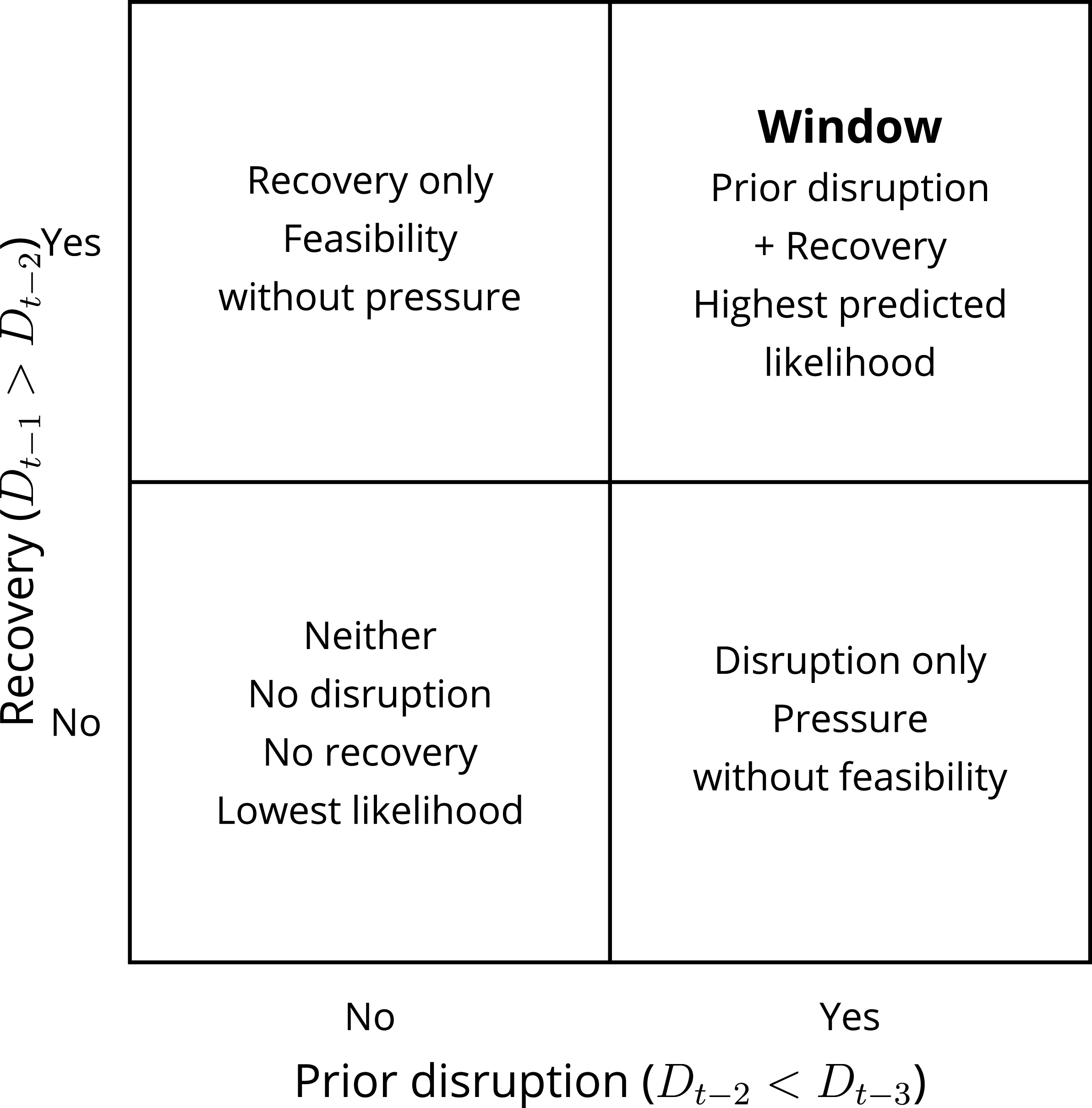
 Dt−2
 Dt−1>Dt−2

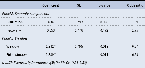
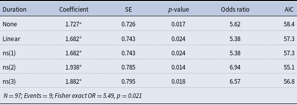
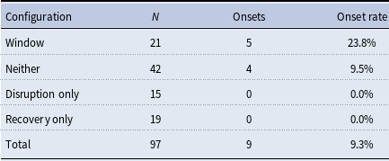
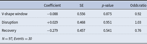
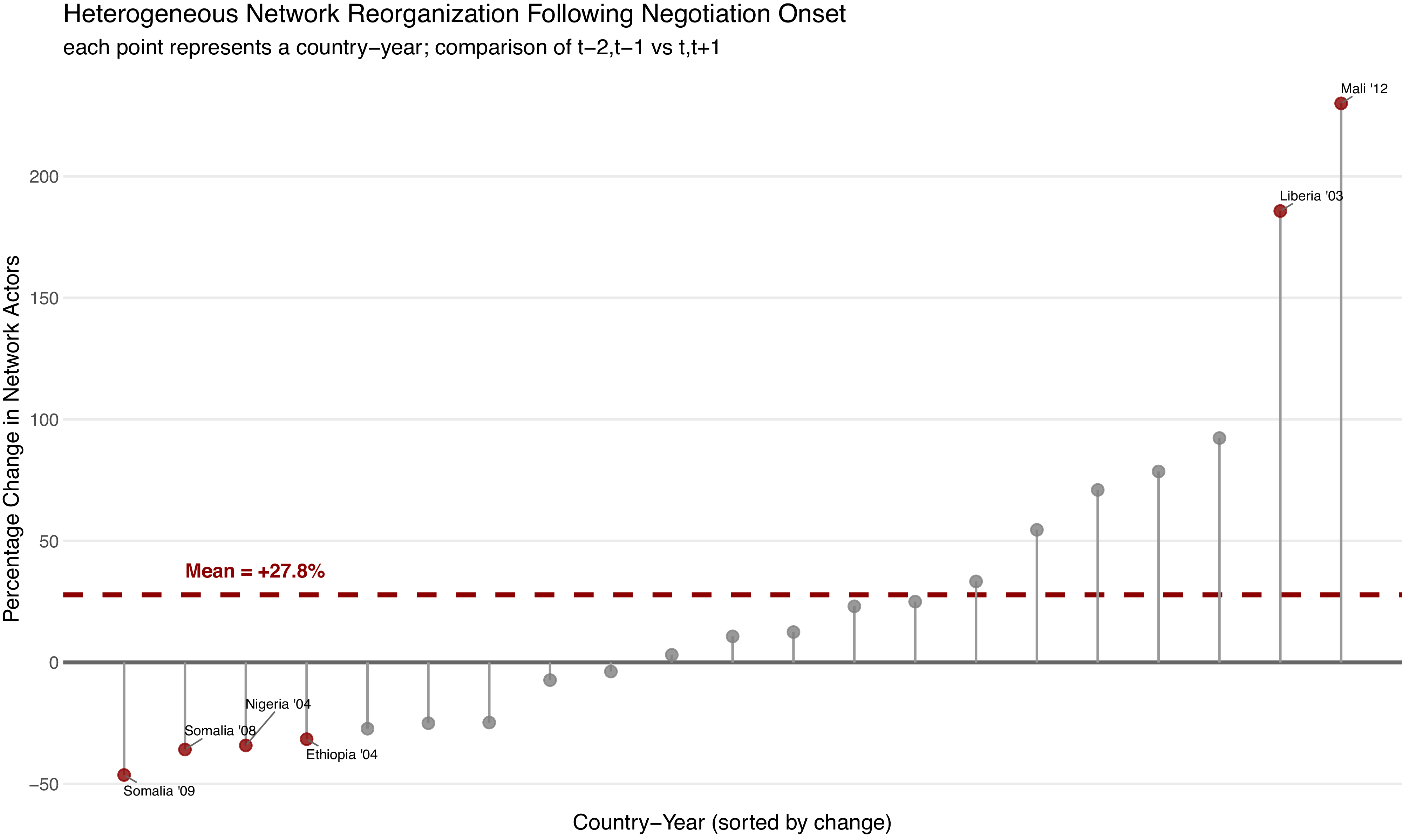
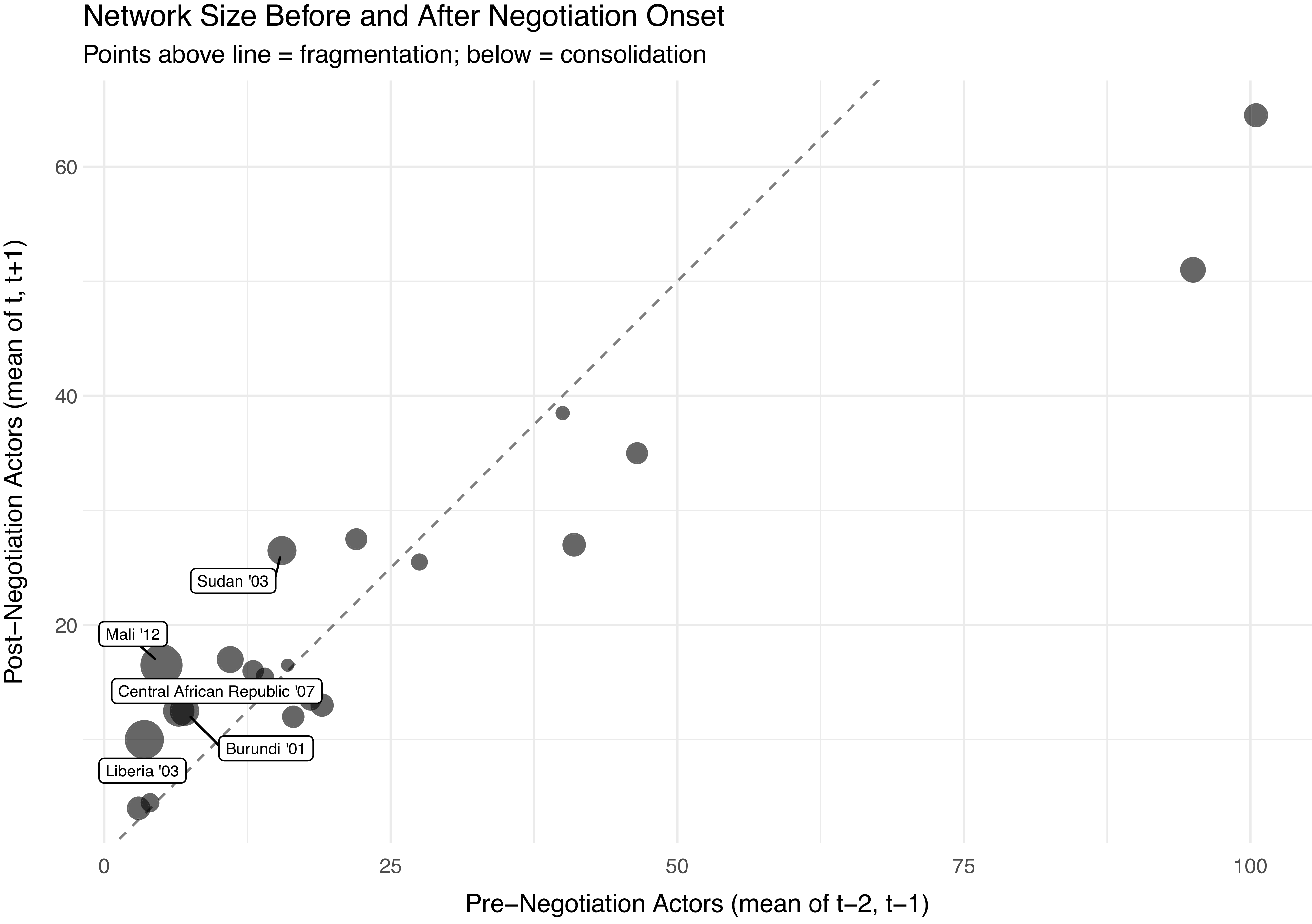
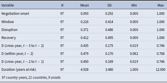
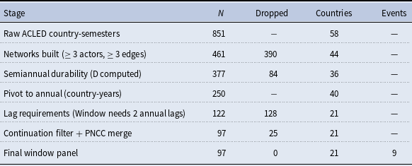
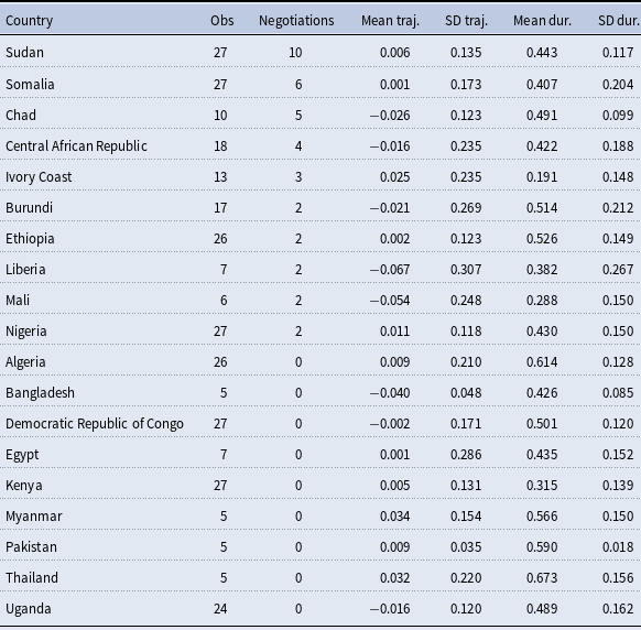
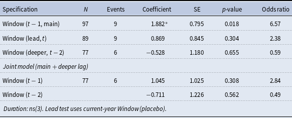
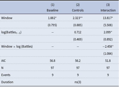
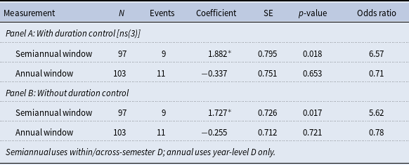

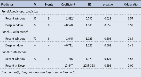
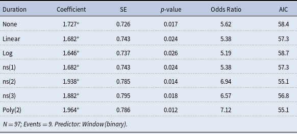
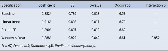
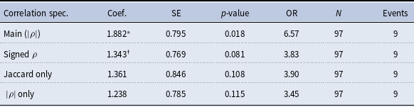
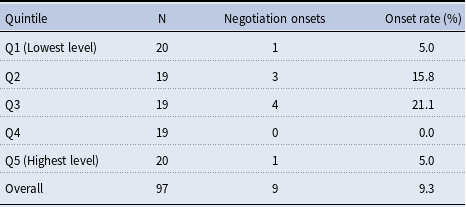
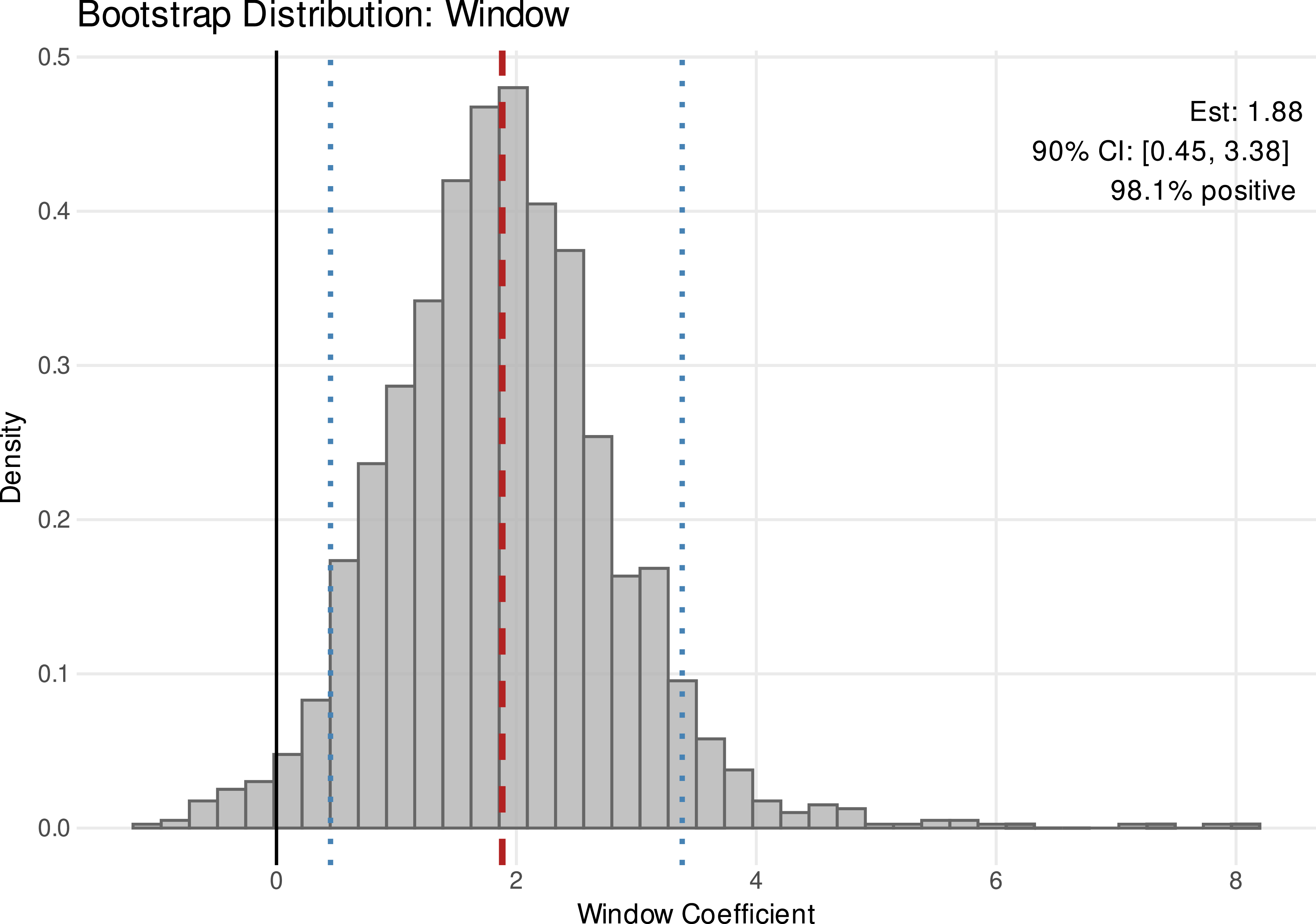
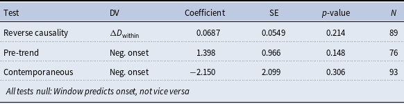
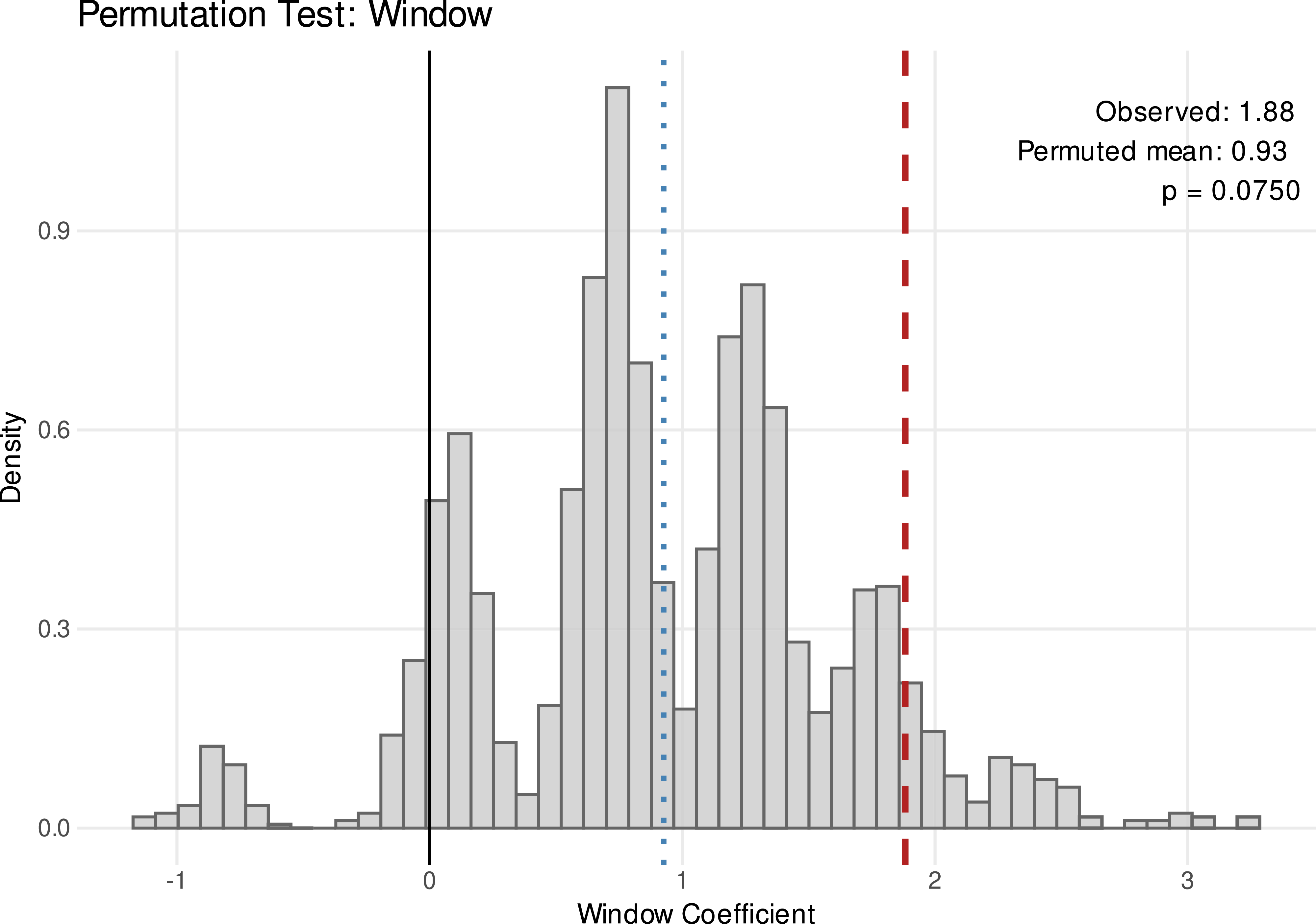
 p=0.075
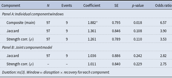

 |

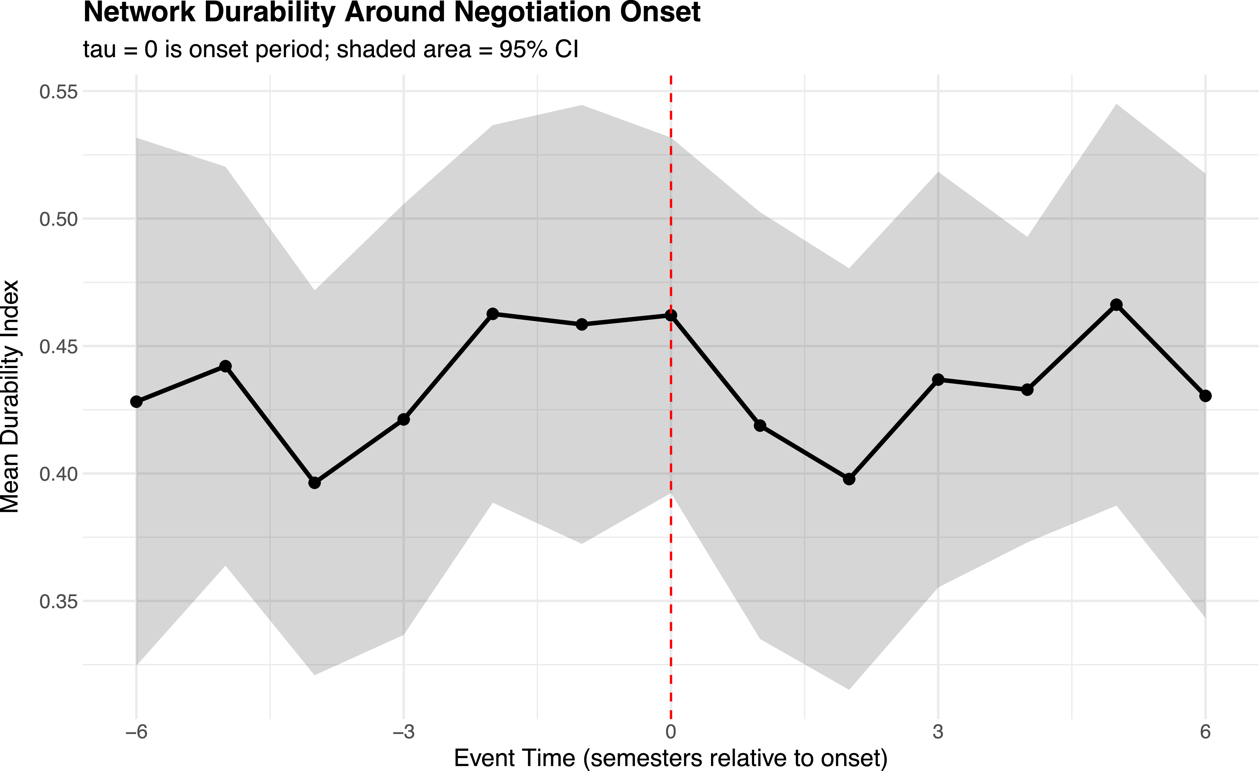
 τ∈[−6,+6]
 τ=0

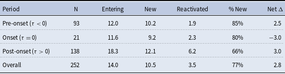

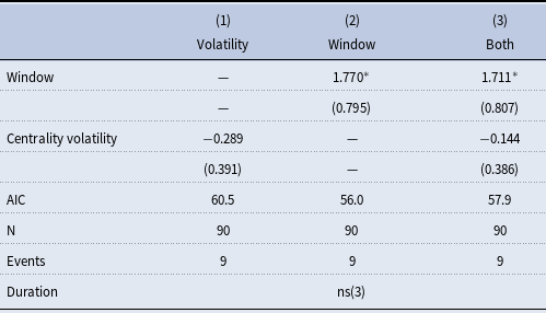
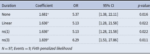
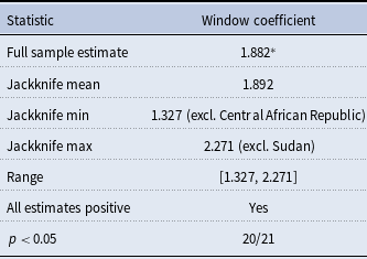
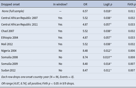
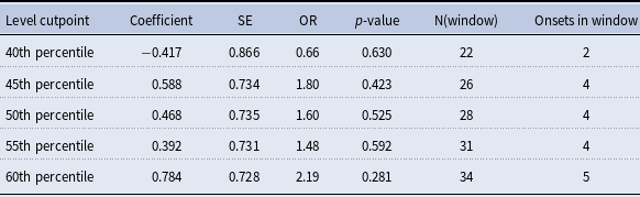

 Open access

