INTRODUCTION
Permanent grasslands still cover a large part of the utilized agricultural area (UAA) in Europe (57·6 Mha, 0·34 UAA) and in France (8·4 Mha, 0·30 UAA) (EC Eurostat 2012). However, the grassland acreage has declined steadily over the last 30 years. European Union policy tries to maintain permanent grassland in the landscape, especially because of their environmental utility (biodiversity, water quality, soil erosion, landscape aesthetics, etc.). In addition, their economic utility as a cheap food resource in some production systems may be considerable. This trend is mostly explained by competition for land use between forage and crop production, and the development of maize silage. However, a lack of knowledge about permanent grassland value and optimal management can also explain the decline of European permanent grassland, as suggested by Huyghe (Reference Huygue2008). Therefore there is a need to quantify permanent grassland forage yield and quality more precisely, and to determine the key factors determining the value of permanent grassland.
Quantity and quality of forage provided by permanent grassland rely mainly on the annual level and seasonal dynamics of biomass production, estimated by dry matter (DM) yield (Daccord et al. Reference Daccord, Wyss, Kessler, Arrigo, Rouel, Lehmann and Jeangros2006), and grass nutritive value, estimated by crude protein content (CP) and organic matter digestibility (OMD) (Demarquilly & Andrieu Reference Demarquilly, Andrieu and Agabriel1988; Van Soest Reference Van Soest1994). Biomass production and grass nutritive values are influenced by different factors such as weather, soil and vegetation characteristics (Buxton Reference Buxton1996; Louault et al. Reference Louault, Pillar, Aufrère, Garnier and Soussana2005; Duru et al. Reference Duru, Cruz and Theau2010). Also, the diversity of the vegetation composition affects the forage quantity or quality of permanent grassland (Bruinenberg et al. Reference Bruinenberg, Valk, Korevaar and Stuik2002; Baumont et al. Reference Baumont, Pelletier, Peccatte, Aufrère, Delaby, Surault, Niderkorn and Andueza2008).
The complexity of vegetation in permanent grassland can be described by botanical and functional composition (Grime et al. Reference Grime, Hodgson and Hunt1979; Duru et al. Reference Duru, Theau, Cruz, Jouany, Therond, Al Haj Khaled and Ansquer2007; Maire Reference Maire2009). Botanical composition gives information on the presence and dominance of species, but requires the ability to recognize them (Maire Reference Maire2009), whereas functional composition merges species into functional types based on their life traits (Violle et al. Reference Violle, Navas, Vile, Kazakou, Fortunel, Hummel and Garnier2007). These life traits, measured at the species level, are often listed in databases (Kleyer et al. Reference Kleyer, Bekker, Knevel, Bakker, Thomson, Sonnenschein, Poschold, Van Groenendael, Klime, Klimesova, Klotz, Rusch, Hermy, Adriaens, Boedeltje, Bossuyt, Dannemann, Endels, Götzenberger, Hodgson, Jackel, Khün, Kunzmann, Ozinga, Römermann, Stadler, Schlegelmilch, Steendam, Tackenberg, Wilmann, Cornelissen, Eriksson, Garnier and Peco2008). Plant life traits can be classified into ‘effect traits’ (those affecting features such as production or quality) and ‘response traits’ (those related to factors such as soil or weather conditions) (Pavlu et al. Reference Pavlu, Hejcman, Pavlanduring and Gaisler2007; Rose et al. Reference Rose, Rubarth, Hertel and Leuschner2013). For example, Pontes et al. (Reference Pontes, Soussana, Louault, Andueza and Carrère2007) demonstrated that grass digestibility increased with the specific leaf area and declined with leaf DM content. Plant life traits can be averaged at plant community or habitat level (Violle et al. Reference Violle, Navas, Vile, Kazakou, Fortunel, Hummel and Garnier2007): at these scales, a weighted average value of plant traits encapsulates the effect of weather and nutrients (Cordlandwehr et al. Reference Cordlandwehr, Meredith, Ozinga, Bekker, Van Groenendael and Bakker2013). Cordlandwehr et al. (Reference Cordlandwehr, Meredith, Ozinga, Bekker, Van Groenendael and Bakker2013) showed that this might result in low accuracy of averaged traits expected for predicting ecosystem services such as biomass production at plant community level. However, when external drivers are taken in account, other studies demonstrated a good prediction of grass production and quality using plant traits at this scale (Jouven et al. Reference Jouven, Carrère and Baumont2006; Duru et al. Reference Duru, Al Haj Khaled, Ducourtieux, Theau, De Quadros and Cruz2009).
Concerning grassland, a functional classification based on plant growth strategies, fertility level and defoliation rate was proposed by Duru and Cruz (Cruz et al. Reference Cruz, Duru, Therond, Theau, Ducourtieux, Jouany, Al Haj Khaled and Ansquer2002, Reference Cruz, Theau, Lecloux, Jouany and Duru2010; Louault et al. Reference Louault, Pillar, Aufrère, Garnier and Soussana2005; Duru et al. Reference Duru, Cruz, Al Haj Khaled, Ducourtieux and Theau2008). This classification distinguishes five plant functional types (PFT) based on grass features (Cruz et al. Reference Cruz, Duru, Therond, Theau, Ducourtieux, Jouany, Al Haj Khaled and Ansquer2002, Reference Cruz, Theau, Lecloux, Jouany and Duru2010): species adapted to fertile soil and frequent defoliation are characterized by a high specific leaf area and low leaf DM content. Conversely, species adapted to infertile soils show the low specific leaf area and high leaf DM content. Although the classification was designed for grasses, similarity has been demonstrated between grass and dicotyledonous species characteristics within a grassland community (Ansquer et al. Reference Ansquer, Duru, Theau and Cruz2009). However, the importance of the proportions of legumes and forbs on permanent grassland quality has been demonstrated (Huyghe et al. Reference Huygue, Baumont and Isselstein2008). It may thus be useful to study functional group composition (proportions of grasses, legumes and forbs).
Other vegetation criteria that characterize the sward globally, such as mean phenological development or mean dry matter content (DMC) (Violle et al. Reference Violle, Navas, Vile, Kazakou, Fortunel, Hummel and Garnier2007) may also be correlated with biomass production or forage quality (Demarquilly & Jarrige Reference Demarquilly, Jarrige and Demarquilly1981; Moore & Moser Reference Moore and Moser1995; Buxton Reference Buxton1996). They also take into account intrinsic plant properties or environmental conditions (soil and weather conditions) (Skinner et al. Reference Skinner, Gustine and Sandersson2004) and can be used as a proxy for plant functional traits. Because they are more easily measured, these descriptors can be tested at the community level.
These vegetation characteristics have been used mostly over a narrow range of conditions, in experiments located either at a single site or in a small region (Louault et al. Reference Louault, Pillar, Aufrère, Garnier and Soussana2005; Duru et al. Reference Duru, Cruz, Al Haj Khaled, Ducourtieux and Theau2008; Andueza et al. Reference Andueza, Cruz, Farruggia, Baumont, Picard and Michalet-Doreau2010; Michaud et al. Reference Michaud, Andueza, Picard, Plantureux and Baumont2012a). On a broad scale, environmental and management conditions show more variability and may thus have more influence on forage value (Michaud et al. Reference Michaud, Plantureux, Amiaud, Carrère, Cruz, Duru, Dury, Farruggia, Fiorelli, Kerneis and Baumont2012b).
The aim of the current study was to investigate the extent to which biomass production and grass nutritive value are explained by functional composition over a wide range of conditions. Previous studies on grassland generally focused on a few situations, as in the work of Cordlandwehr et al. (Reference Cordlandwehr, Meredith, Ozinga, Bekker, Van Groenendael and Bakker2013) with two grassland sites: a wet meadow and a salt marsh. Climatic data were introduced in order to determine the relative contributions of vegetation characteristics and weather to grassland performance. In order to determinate the best characteristics of the vegetation to predict biomass production and nutritive value, two prediction models were considered: (i) botanical families/PFT of grasses and (ii) botanical families/proxy for PFT (phenological development and DMC) measured in situ. More specifically, two questions were addressed:
• Do the same variables explain biomass and sward nutritive value?
• Do the same variables explain quantity or quality during the growing season?
To this end, data and grass samples collected in an original set of a wide range of permanent grassland in France were analysed, taking into account management variability and environmental conditions. The current study may help to generalize these links for a wide range of management and environmental conditions.
MATERIALS AND METHODS
Sampling design
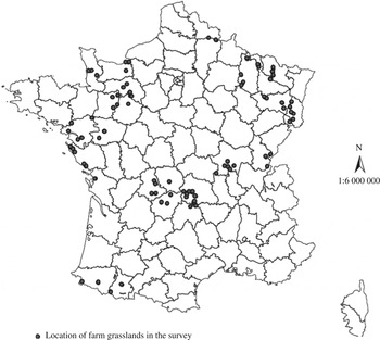
A set of 190 French permanent grasslands was selected from 1500 listed by a survey conducted in 2008 on 78 farms (Fig. 1, for more details about the range of management, and edaphic and climatic conditions see Michaud et al. Reference Michaud, Plantureux, Amiaud, Carrère, Cruz, Duru, Dury, Farruggia, Fiorelli, Kerneis and Baumont2012b). In all the farms the forage production area consisted of a minimum of 0·50 permanent grassland for >10 years. Farms were chosen to represent a diversity of production systems in different types of region: dairy or beef cattle production, milk or meat sheep production. First, permanent grasslands were sampled by considering variability of management practices: type of use (grazed only, cut only, grazed and cut), intensity of use (number of cuts, livestock density), type and amount of fertilization. Second, soil and climatic conditions were considered in order to obtain a broad range of environmental conditions. The set included most soil and climatic areas from Atlantic to Alpine conditions, and covered most of the existing permanent grassland types in France. The altitude ranged from sea level to 2000 m a.s.l. Only Mediterranean areas of dry scrubland were excluded.
Location of permanent grasslands in the set.

Data collection
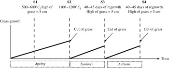
The dominant flora of each permanent grassland, as represented by a homogeneous plant community (in terms of vegetation structure and floristic composition) of about 1 ha, was determined and mapped. Within this area, three quadrats (1·5×3 m) were protected from grazing or cutting by the farmer. All the samples were taken in these three quadrats following a standard procedure on all sites. The experiment lasted for 2 years (2009/10), with four samplings per year (Fig. 2). The timing of the first two samplings in each year was based on thermal time (see below for details) (De Montard Reference De Montard1981; Rossignol et al. Reference Rossignol, Andueza, Carrère, Cruz, Duru, Fiorelli, Michaud, Plantureux, Pottier and Baumont2013) and that for the second and third cycles on regrowth days (RD, expressed in days) (De Montard Reference De Montard1981; Niqueux & Arnaud Reference Niqueux and Arnaud1981):
• Two samplings in spring: one at the beginning of spring between 500 and 600 °C days, counted from 1 February, to obtain information for early use (S 1) (grazing, silage), and one at the end of spring between 1100 and 1200 °C days from 1 February, to obtain information for later use (S 2) (hay cut, late grazing). These temperature sums (ST) were calculated as accumulated mean daily temperatures (0 °C<T<18 °C), following the recommendations of Theau & Zerourou (Reference Theau, Zerourou, Cruz, Jouany and Theau2008).
• Two samplings for regrowths: one in summer, (S 3, 40 days after S 2) and one in autumn (S 4, 40 days after S 3).
Sampling in spring was based on thermal time because of the rapid temperature changes at that time and had to take account of the availability of the technical staff doing the sampling. They came from different parts of France and underwent a 2-day training session to ensure that they all followed the same sampling protocol.
Grass data collection procedure during the year, considering sum of temperature (°C days) or regrowth days (days). Four samples were taken: one at the beginning of spring (S1), one at the end of spring (S2), one during summer (S3) and one during autumn (S4).

Water balance (WB) was taken into account and expressed as water shortage: it was calculated as the difference between evapotranspiration and rainfall. For this data from 2009 and 2010 were used, supplied by Météo France for the weather stations closest to the studied grasslands. Daily rainfall and evapotranspiration data were summed for the periods from 1 February till S 1 and S 2 for spring and from S 2 to S 3 and S 3 to S 4 for regrowths.
At each sampling, two sub-samples were collected:
• One sub-sample for the study of functional composition and sward characteristics;
• One sub-sample for the study of biomass production and grass nutritive value.
Vegetation characteristics
Proportions of grasses, legumes and forbs
Sub-samples collected for functional composition analyses were frozen at −20 °C. After thawing, proportions of grasses, legumes and forbs were estimated visually for all samples. The estimation, based on volume, was made by the same staff during the 2 years.
Phenological development
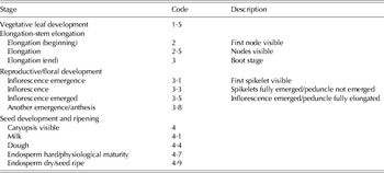
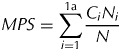
For spring samples (S 1, S 2), grass plant phenology and PFT were determined on 40 tillers on the frozen sub-sample. Each tiller was classified according the 13 vegetation stages defined from an adaptation of the method proposed by Moore et al. (Reference Moore, Moser, Vogel, Waller, Johnson and Pedersen1991) (Table 1). Grass plant phenology was determined by the medium plant stage (MPS) for each sample and calculated as follows:
 $$MPS = \sum\limits_{i = 1}^{1{\rm a}} {\displaystyle{{C_i N_i} \over N}} $$
where C i is the code of stage i as defined in Table 1, N i is the number of plants in stage I, and N is the total number of plants.
Definition of the 13 plant stages used to characterize medium plant stage of the grasslands (adapted from Moore et al. Reference Moore, Moser, Vogel, Waller, Johnson and Pedersen1991)

Plant functional type of grasses
Each tiller used for phenological development determination was identified according to a classification proposed by Cruz et al. (Reference Cruz, Theau, Lecloux, Jouany and Duru2010): PFT A and B, composed of early species, are characterized by high biomass production and high nutritive value, with a rapid decline in biomass over time. Plant functional types C and D, composed of late species, are characterized by low biomass production and low digestibility, with a steadier production over time. Recently, PFT b was added to the characterized species list, found on soils of medium fertility and with later phenology than PFT A and B (Cruz et al. Reference Cruz, Theau, Lecloux, Jouany and Duru2010). Plant functional types A, B, b, C and D, were considered in the current study.
Dry matter content
The other sub-sample of the fresh harvest biomass was weighed and dried at 60 °C for 72 h to determine DMC.
Biomass production and grass nutritive value
By means of the dried sample and the DMC, the dry matter yield (DMY) of each permanent grassland (t DM/ha) was calculated for all cutting dates in order to quantify biomass production. The height of cut was 5 cm.
The nutritive value of the herbage harvested was assessed using the 1221 sub-samples collected for DMY for each of the 190 permanent grasslands, and for the four cutting dates over 2 years. The lack of grass during summer due to severe dry conditions was the major cause of there being fewer samples than planned (1221 instead of 1520=190×4×2 samples). The sub-samples were ground using a sample mill through a 0·8 mm screen. Each herbage sub-sample was analysed using near-infrared reflectance spectroscopy to determine pepsin–cellulase DM digestibility and CP. Near-infrared spectra were collected with a monochromator (FOSS-NIRSystems 6500, Silver Spring, MD, USA), which scanned the spectral range 400–2500 nm. All spectra and reference data were recorded and managed with WINISI Version 1.6 software (Infrasoft International, Port Matilda, PA, USA). Modified partial least-square calibration equations were developed using samples selected from the total spectral population collected (Shenk & Westerhaus Reference Shenk and Westerhaus1991). The calibration dataset was analysed for pepsin–cellulase DM digestibility (Aufrère & Demarquilly Reference Aufrère, Demarquilly and Desroches1989) and CP (using Kjeldahl N×6·25) of herbage. The statistical parameters of the calibration models obtained for pepsin–cellulase–DM digestibility and CP of herbage were as follows: number of samples: 496 and 478, s.e. of cross-validation: 0·021 g/g and 4·19 g/kg DM, and R 2 value of cross-validation, 0·97 and 0·99, respectively. Organic matter digestibility was calculated from pepsin–cellulase DM digestibility using the equation proposed by Aufrère et al. (Reference Aufrère, Baumont, Delaby, Peccatte, Andrieu, Andrieu and Dulphy2007).
Data analysis
The statistical analysis aimed at quantifying links between forage value, vegetation characteristics, climatic data and year of measurement.
Forage value was characterized by biomass production and nutritive value (OMD and CP). Vegetation characteristics considered as explanatory variables were: botanical family (proportion of grasses, legumes and forbs), PFT of grasses (PFT A, B, b, C and D), MPS and DMC. For spring analyses (S1 and S2) all the variables were considered, but for regrowth analyses (S3 and S4) only proportion of grasses, legumes and forbs, and DMC were considered as PFT and MPS were not measured. Climatic variables were WB and ST in spring (S1 and S2), RD for S3 and S4.
First, correlation between the variables that characterized vegetation was tested by statistical treatments with R software package version 3.0.2 (R Development Core Team 2013) in order to select independent variables.
Then, variance–covariance models were established using the general linear model (GLM) procedure. Except year of measurement all variables were continuous (1 d.f.) and all variables were considered as fixed effects in the analysis. Year effect and interactions between continuous variables and year of measurement were systematically tested.
Two types of models were established:
• One with functional composition (botanical family, PFT), climatic variables and year effect;
• One with botanical families and proxy of PFT (MPS and DMC), climatic variables and year effect.
For each type of model one analysis was performed for each of the four measurement periods (S1, S2, S3 and S4). Finally eight models were established for biomass production, as well as for OMD and CP.
RESULTS
Climatic data
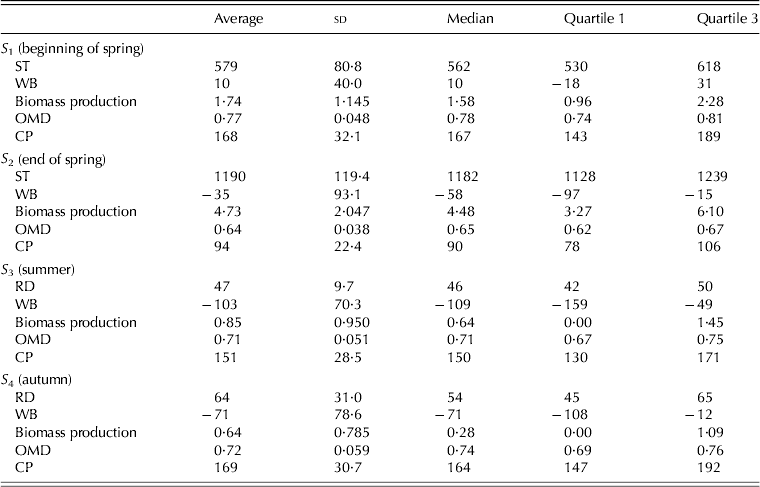
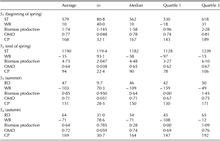
Table 2 shows that most of the sampling dates were included in the planned ST intervals (S1 at 579 °C day and S 2 at 1190 °C day). Water balance was positive at the beginning of spring, with an average of 10 mm, but decreased thereafter: at the end of spring and for the rest of the year it was negative. The water shortage was thus marked from the end of spring, with large regional differences.
Data for the 190 permanent grasslands studied for 2 years: average of 2 years, sd, median and 1 and 3 quartiles for biomass production (t DM/ha), organic matter digestibility (OMD) (g/g) and crude protein content (CP) (g/kg DM). Water balance (WB); sum of temperature (ST) (°C days) and regrowth days (RD) (days) are also described
Data on biomass production, grass nutritive value and vegetation characteristics
Biomass production and grass nutritive value
Mean annual biomass production reached 6·23 t DM/ha (Table 2, sum of S 2+S 3+S 4), and data showed a high variability at different sampling dates. At the beginning of spring (S 1), average biomass production was 1·74 t DM/ha±1·15. The variability of biomass production at the end of spring (S 2) was marked, with an average of 4·73±2·05 t DM/ha. Summer and autumn biomass production were lower, on average 1 t DM/ha. The bottom quarter of permanent grasslands was characterized by no production, while production of the top quarter was about 1·3 t DM/ha.
Concerning grass nutritive value, OMD and CP also showed great variability, more markedly for CP. Organic matter digestibility during spring decreased with time (from 0·77 to 0·64 g/g) (Table 2). The same trend was observed for CP during spring, with a decrease from 168 to 94 g/kg DM (±22·4–32·1 g/kg DM). Summer and autumn permanent grasslands OMD was close to 0·71–0·72±0·051–0·059 g/g. Crude protein was lower in summer than in autumn: 151±28·5 and 169±30·7 g/kg DM, respectively.
Vegetation characteristics
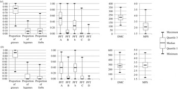
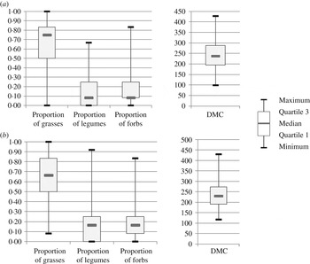
During spring the proportion of grasses remained high. It decreased in summer and autumn around a median of 0·65–0·75 (Figs 3 and 4). Proportions of legumes and forbs then both showed an increase during regrowth periods, to reach a median of 0·17 for legumes and forbs in S 4. The proportion of grasses classified in PFT A and PFT b were the dominant types in the set in spring (Fig. 3): PFT A reached 0·50 (value of median) in S 1 and PFT b 0·40 in S 2. For PFT C, the proportion was low (<0·08) during spring. However, proportions of PFT C higher than 0·50 were found in six permanent grasslands.
Box plot of functional composition description for the 190 permanent grasslands studied over 2 years for: proportions of grasses, legumes and forbs, proportion of plant functional types (PFT) A, B, b, C and D, medium plant stage (MPS), and dry matter content (DMC) (g/kg), and for the beginning of spring (S1) (a) and the end of spring (S2) (b) PFT A and B, composed of early species, are characterized by high biomass production and high nutritive value, with a rapid decline in biomass over time. PFT C and D, composed of late species, are characterized by low biomass production and low digestibility, with a steadier production over time. PFT b, which is found on soils of medium fertility, is characterized by later phenology than PFT A and B.

Box plot of functional composition description for the 190 permanent grasslands studied during two years for: proportions of grasses, legumes and forbs, proportion of plant functional types (PFT) A, B, b, C, D and E, medium plant stage (MPS), and dry matter content (DMC) (g/kg), and for summer (S3) (a) and autumn (S4) (b).PFT A and B, composed of early species, are characterized by high biomass production and high nutritive value, with a rapid decline in biomass over time. PFT C and D, composed of late species, are characterized by low biomass production and low digestibility, with a steadier production over time. PFT b, which is found on soils of medium fertility, is characterized by later phenology than PFT A and B.

Dry matter content was c. 217–276 g/kg (median values) within a year, with an increase at the end of spring (Fig. 4). Grass phenology increased during spring from 2·1 (beginning of elongation) to 3·2 (inflorescence) (value of median) with a high variability in particular because some permanent grasslands stayed at a vegetative stage.
Among vegetation characteristics, statistical analysis of colinearity showed that PFT A was negatively correlated with PFT B, b, C, and D, and was therefore removed from the statistical analysis to avoid redundancy. Also, the proportion of grasses was highly negatively correlated with proportions of both legumes and forbs, which were slightly positively correlated with each other. The proportion of grasses was therefore not retained for statistical analysis for the same reason as PFT A.
Links between vegetation characteristics, climatic data, biomass production and grass nutritive value
Results are presented separately for the two models: model 1 taking into account the proportion of legumes and forbs, and PFT as vegetation characteristics and model 2, taking into account the proportion of legumes and forbs, MPS and DMC as vegetation characteristics. The year effect was significant for most of the models. Moreover interactions were found between vegetation characteristics, ST, WB and year.
Biomass production
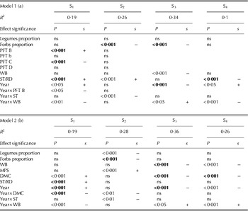
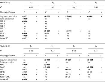
In both models, results of predictions showed that vegetation characteristics and weather data contributed to explain the variability of biomass production throughout the year (Table 3). Vegetation characteristics were illustrated by the proportion of forbs, PFT B and PFT C in model 1 and MPS and DMC in model 2.
Regression results between biomass production (t DM/ha) and vegetation characteristics (proportion of legumes and forbs, plant functional trait B, b, C and D proportion for model 1 (a) and proportion of legumes and forbs, medium plant stage and DM content for model 2 (b)) for spring (beginning S1, end S2), summer (S3) and autumn (S4) samples

PFT, plant functional trait; MPS, medium plant stage; DMC, dry matter content; ST, sum of temperature; RD, regrowth days; WB, water balance; Year, year effect; ns, not significant; s, sign; non-significant interactions are not in the table.
In model 1, the effect of climatic variables was significant and important during the year. The ST effect was positive in spring and negative for autumn regrowth. The WB effect was negative in summer and variable according to year at S1, S3 and S4. There was no effect of WB in spring and autumn. Moreover S 4 was strongly driven by climatic variables with a negative effect (Table 3). In spring, R 2 values of the model indicated that vegetation characteristics and weather explained 0·19 of the variability in biomass production in S1 and 0·26 in S2. Proportion of forbs was the factor best correlated with biomass production (Table 3). The effect of PFT was low and restricted to PFT B (positive effect) and PFT C (negative effect). The contribution made by vegetation characteristics and climatic data to explain biomass production was higher in summer and lower in autumn, i.e. 0·34 for S3 and 0·10 for S4. In S3, it was supported by a negative effect of the proportion of forbs in S3 and no vegetation variable in S4.
In model 2, the weather effect was significant during the year, considering ST, WB or interaction with year. Regrowth was mainly governed by WB (negative effect). In spring, vegetation characteristics and weather explained a part of the variability with R 2 0·19 at S1 and 0·28 at S2. In the beginning of spring, the only effect of vegetation characteristics was a positive effect of DMC. At the end of spring, a negative effect was found for the proportion of forbs and legumes and a positive effect for MPS. The contribution of vegetation characteristics in summer and autumn was only illustrated by a negative effect of DMC.
Organic matter digestibility
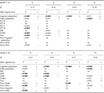
In both models, vegetation characteristics and weather helped to explain the variability of OMD throughout the year. Vegetation characteristics were characterized by the effects of the proportion of legumes and forbs in both models, considering MPS and DMC in model 2 (Table 4).
Regression results between organic matter digestibility (OMD in g/g) and vegetation characteristics (proportion of legumes and forbs, plant functional trait B, b, C and D proportion for model 1 (a) and proportion of legumes and forbs, medium plant stage and dry matter content for model 2 (b)) for spring (beginning S1, end S2), summer (S3) and autumn (S4) samples

PFT, plant functional trait; MPS, medium plant stage; DMC, dry matter content; ST, sum of temperature; RD, regrowth days; WB, water balance; Year, year effect; ns, not significant; s, sign; non-significant interactions are not in the table.
In model 1, the effect of weather was significant. The ST effect was large and negative in spring. The WB effect was positive at the end of spring. Year-to-year variability of WB was apparent at the beginning of spring and in autumn, with a negative effect in the beginning of spring and a positive effect in autumn of the second year. In spring, vegetation characteristics and weather explained much of the variability with R 2 0·21 S1 and 0·26 in S2 (Table 4). The proportion of legumes and forbs explained much of the variation in OMD and particularly that of legumes. The effect of the proportion of forbs was negative in the beginning of spring and positive at the end of spring. The influence of the proportion of legumes varied from year to year. The only PFTs to have an effect were PFT C (negative effect) and PFT D (positive effect) at the beginning of spring. The contribution of the proportion of legumes and forbs was substantial and positive for regrowths too.
With model 2, the effect of weather was less (Table 4). A year effect with WB was only found at S1 and S4. The ST effect was only significant for S 4. In spring, vegetation characteristics and weather explained much of the variability with R 2 0·22 at S1 and 0·41 at S2. The effect of the proportion of legumes was large and positive. However, the effect of the proportion of forbs was lower and not significant at the end of spring and in summer. Medium plant stage and DMC had a strongly negative effect on OMD. Moreover, the effect of legumes and proportion of forbs was large and positive for OMD of the regrowths. The negative effect of DMC helped to explain this.
Crude protein content
With both models, the predictions show that vegetation characteristics and weather helped to explain CP levels, particularly for regrowths. Vegetation characteristics were illustrated by the effect of the proportion of legumes in both models, plus MPS and DMC effects in model 2 (Table 5).
Regression results between crude protein content (CP in g/kg DM) and vegetation characteristics (proportion of legumes and forbs, plant functional trait B, b, C and D proportion for model 1 (a) and proportion of legumes and forbs, medium plant stage and dry matter content for model 2 (b)) for spring (beginning S1, end S2), summer (S3) and autumn (S4) samples.

PFT, plant functional trait; MPS, medium plant stage; DMC, dry matter content; ST, sum of temperature; RD, regrowth days; WB, water balance; Year, year effect; ns, not significant; s, sign; non-significant interactions are not in the table.
With model 1, the effect of weather was small. Water balance was shown to have an effect at the end of spring and in summer and an effect of ST in spring (Table 5). There was no effect of weather at S4. In spring, vegetation characteristics and weather explained part of the variability of CP (R 2 0·17 at S1 and 0·20 at S2). Legumes had a large positive effect on CP. In the beginning of spring, there was a negative effect of the proportion of forbs and a positive effect of PFT B. The proportion of legumes was the only vegetation characteristic to explain CP at the end of spring and for regrowths.
With model 2, the effect of weather was much the same except that the ST effect was not significant at the end of spring but large in autumn. In spring, vegetation characteristics and weather explained part of the variability (R 2=0·13 at S1 and 0·37 at S2). Medium plant stage was inversely related to CP at S1, while the proportion of legumes, MPS and DMC helped to explain the CP data at the end of spring (positive effect of legumes and negative effect of DMC and MPS). Regrowth CP was mainly explained by a positive effect of legumes and a negative effect of DMC.
DISCUSSION
Variability of data
The features of the dataset have been described by Michaud et al. (Reference Michaud, Plantureux, Amiaud, Carrère, Cruz, Duru, Dury, Farruggia, Fiorelli, Kerneis and Baumont2012b). It was created to account for the variability of practices and environmental conditions found in the large geographical region studied. The proportions of permanent grasslands classified as grazed only (0·44), cut only (0·13), and mixed grazed and cut (0·43) in the dataset is close to the French national average (Rabaut Reference Rabaut2000). The variability in management conditions associated with the geographical distribution offers a broad range of conditions. This could help to explain the variability of vegetation characteristics and forage value data, as shown by several authors (Bruinenberg et al. Reference Bruinenberg, Valk, Korevaar and Stuik2002; Daccord et al. Reference Daccord, Wyss, Kessler, Arrigo, Rouel, Lehmann and Jeangros2006; Baumont et al. Reference Baumont, Pelletier, Peccatte, Aufrère, Delaby, Surault, Niderkorn and Andueza2008).
The variability of data was greater for biomass production than for nutritive value. The mean sd lies between 0·43 and 1·23 t/ha for biomass production. This variability could be explained by environmental conditions: biomass production is affected by the weather (notably rainfall) and by management practices (Jeangros & Schmid Reference Jeangros and Schmid1991; Isselstein Reference Isselstein1993). Also, measurements of biomass production were made on a small quadrat (3×0·49 m2 for grassland). A larger sampling area might improve measurement precision (Corral & Fenlon Reference Corral and Fenlon1977; Mosimann Reference Mosimann2001). As for nutritive value, CP showed higher variability than OMD: from 0·19 to 0·24 g/kg DM for CP and from 0·06 to 0·08 g/g for OMD (Table 2). Fertilization rate could help to explain the variability of CP (Dirienzo et al. Reference Dirienzo, Webb and Brann1991; Isselstein Reference Isselstein1993). Finally, the variability of vegetation characteristics and forage value was taken into account in the analyses by taking samples at the same temperature sums accumulated from 1 February (Rossignol et al. Reference Rossignol, Andueza, Carrère, Cruz, Duru, Fiorelli, Michaud, Plantureux, Pottier and Baumont2013).
Models linking vegetation characteristics, climatic data, biomass production and nutritive value
Permanent grassland production and forage quality can be explained by three types of factors: soil and weather conditions, management and vegetation characteristics. Several authors have studied the links between forage value and vegetation characteristics (Demarquilly & Andrieu Reference Demarquilly, Andrieu and Agabriel1988; Bornard & Dubost Reference Bornard and Dubost1992; Arzani et al. Reference Arzani, Zohdi, Fish, Zahedi Amiri, Nikkhah and Wester2004; Andueza et al. Reference Andueza, Cruz, Farruggia, Baumont, Picard and Michalet-Doreau2010) or environmental conditions (Topp & Doyle Reference Topp and Doyle1996; Hermann et al. Reference Hermann, Kelm, Kornher and Taube2005), but the relative effects of these categories of factors have seldom been estimated. A key goal of the current study was to estimate the effects of vegetation characteristics and climatic data together, and the results suggest that they help to explain much of the variance of the data. Thus, for model 1, R 2 values reached 0·49 for OMD and CP, but were lower for biomass production: from 0·10 to 0·34. For model 2, R 2 values were similar to those for model 1: they reached 0·51 for OMD and CP and 0·36 for biomass production. As suggested above, the greater dependence of biomass production on environmental conditions and management practices could explain these results (Jeangros & Schmid Reference Jeangros and Schmid1991; Isselstein Reference Isselstein1993). The R 2 of models were quite similar for first cycle and for regrowths but the effect of variables was different. Regrowth was mainly explained by the weather as demonstrated by Kowalenko & Bittman (Reference Kowalenko and Bittman2000) and Jing et al. (Reference Jing, Bélanger, Baron, Bonesmo, Virkajarvi and Young2012). The fact that vegetation variables are less influential for regrowths than for the first cycle can explain these results.
In addition, the quantity and quality of forage are explained by similar variables: mainly the proportion of legumes for model 1 and the proportion of legumes, MPS and DMC for model 2, although the contribution of variables changes with the seasons. For some samples, other variables help to explain biomass production or grass nutritive value, such as the proportion of forbs for OMD in model 1 and in part in model 2, as demonstrated by Andueza et al. (Reference Andueza, Cruz, Farruggia, Baumont, Picard and Michalet-Doreau2010).
Climatic data
The effect of weather on biomass production was considerable during the year. Water balance was shown to have an effect in summer, which is linked to dry conditions during this period. Regrowths seem to be more affected by weather conditions than the first cycle (Kowalenko & Bittman Reference Kowalenko and Bittman2000; Jing et al. Reference Jing, Bélanger, Baron, Bonesmo, Virkajarvi and Young2012). Nutritive value was lower, due to the weather: the negative effect of ST on OMD could be ontogenetic (Baumont et al. Reference Baumont, Pelletier, Peccatte, Aufrère, Delaby, Surault, Niderkorn and Andueza2008). The positive effect of WB on nutritive value could be explained by the development of leaves in response to water.
Proportion of grasses, legumes and forbs
The effect of proportion of grasses was not included in the current study in order to avoid redundancy, but its effect on biomass production has been demonstrated (Cruz et al. Reference Cruz, Duru, Therond, Theau, Ducourtieux, Jouany, Al Haj Khaled and Ansquer2002, Reference Cruz, Theau, Lecloux, Jouany and Duru2010). Introducing botanical families in the analyses helps to show their effect on biomass production and nutritive value, and particularly the effect of dicotyledons, despite their low proportion. In the current study, their proportion was less than 0·17 during the 2 years of study. Although a similarity between grasses and dicotyledons was shown by Ansquer et al. (Reference Ansquer, Duru, Theau and Cruz2009), the current study demonstrates the importance of taking botanical families into account, particularly for the prediction of nutritive value.
The negative effect of legumes and forbs on biomass production in both models could be explained by plant size. Their contribution to biomass production was lower than that of grasses and particularly legumes, but they do have a positive effect on the quality of permanent grassland (Gierus et al. Reference Gierus, Kleen, Loges and Taube2012), because of their higher proportion of leaves (Baumont et al. Reference Baumont, Pelletier, Peccatte, Aufrère, Delaby, Surault, Niderkorn and Andueza2008). The effects of forbs on OMD may differ for the two models. Daccord et al. (Reference Daccord, Wyss, Kessler, Arrigo, Rouel, Lehmann and Jeangros2006) classified forbs into two categories: stemmy and leafy forbs. Leafy forbs such as Taraxacum could help to improve OMD; their high proportion in the permanent grasslands in the dataset could explain this effect (Michaud et al. Reference Michaud, Plantureux, Amiaud, Carrère, Cruz, Duru, Dury, Farruggia, Fiorelli, Kerneis and Baumont2012b). By contrast, stemmy forbs, for example Apiaceae, will decrease herbage digestibility.
Plant functional types and proxy of plant functional types
Plant functional types were only used for model 1. The contribution of the PFT proportion in prediction models was small. The dataset was characterized by a high proportion of PFT A and PFT b. This could be explained by the construction of the dataset: permanent grasslands are derived from farming systems, which use them to feed animals at grazing or by harvesting forage. However, a gradient of contrasting PFT composition in permanent grasslands was obtained in the dataset according to altitude. Permanent grasslands from mountains are characterized by a high proportion of PFT C (Duru et al. Reference Duru, Cruz, Al Haj Khaled, Ducourtieux and Theau2008). In order to avoid redundancy, PFT A was not introduced in the analyses, but the positive effect on biomass production was demonstrated (Cruz et al. Reference Cruz, Duru, Therond, Theau, Ducourtieux, Jouany, Al Haj Khaled and Ansquer2002, Reference Cruz, Theau, Lecloux, Jouany and Duru2010).
Plants of PFT B help to explain biomass production, because of their intrinsic properties: they are well-adapted to fertile soils and frequent or less frequent defoliation, and are characterized by high specific leaf areas and low leaf DMC, favouring fast regrowth after defoliation (Cruz et al. Reference Cruz, Duru, Therond, Theau, Ducourtieux, Jouany, Al Haj Khaled and Ansquer2002, Reference Cruz, Theau, Lecloux, Jouany and Duru2010; Louault et al. Reference Louault, Pillar, Aufrère, Garnier and Soussana2005). In contrast, PFT C showed a marked negative effect on OMD consistent with previous observations at the sward level (Michaud et al. Reference Michaud, Andueza, Picard, Plantureux and Baumont2012a). Functional traits of plants belonging to PFT C, in particular their high DMC, help to explain this effect (Duru et al. Reference Duru, Theau, Cruz, Jouany, Therond, Al Haj Khaled and Ansquer2007; Cruz et al. Reference Cruz, Theau, Lecloux, Jouany and Duru2010). Finally, the small contribution of PFT towards explaining biomass and nutritive value variability could be related to the variability of plant traits of ecotypes classified in a given PFT over a wide range of environmental conditions.
Sward proprieties were estimated only for model 2. The effect of MPS on biomass production and nutritive value in spring was marked. Medium plant stage reflects the phenology of species, and their development in time. The growth of leaves and stems helps to increase biomass production (Jeangros & Amaudruz Reference Jeangros and Amaudruz2005; Michaud et al. Reference Michaud, Andueza, Picard, Plantureux and Baumont2012a), but lowers nutritive value (Jeangros & Amaudruz Reference Jeangros and Amaudruz2005). Compared with PFT, MPS determination gives more precise information on the actual sward phenology. The negative effect of DMC on regrowths of biomass production and nutritive value could be explained by intrinsic proprieties of species. Species with high leaf DMC are less productive and have lower digestibility (Cruz et al. Reference Cruz, Duru, Therond, Theau, Ducourtieux, Jouany, Al Haj Khaled and Ansquer2002, Reference Cruz, Theau, Lecloux, Jouany and Duru2010). At the sward level, the determination of DMC should reflect the proportions of stems and cell walls, and thus be an indicator of nutritive value, easy to measure over a wide range of environmental and management conditions.
In the current paper, these two types of vegetation characteristics were tested to evaluate the quality and quantity of permanent grasslands. The R 2 values of the two models were similar. Thus DMC and MPS seemed to be good predictors of quality and quantity of permanent grasslands. Unlike PFT, they take account of soil and weather conditions besides the intrinsic characteristics of the species. The choice of PFT or a proxy for it could depend on ease of measurement, which is where DMC scores.
CONCLUSION
Over a wide range of environmental and management conditions, vegetation characteristics and weather explained almost half of the variance of forage quality and 20–40% of the variance of biomass production. The effect of weather was important, particularly for regrowths. Composition in terms of botanical families, plant stage and sward DMC were the common variables that explained both biomass production and nutritive value during the growing season with both models. Biomass production was mainly explained by the proportion of legumes and forbs, MPS and DMC. Grass nutritive value was related to the same factors, including PFT. Increasing proportions of dicotyledonous plants, legumes and forbs reduced biomass production, but improved the nutritive value of the herbage. Even though the contribution of grass PFTs was lower in models, the current study confirms the role of the proportion of PFT C on digestibility. The current study also shows that the direct assessment of sward phenology and DMC may help to explain biomass production and nutritive value just as well as the model in which grasses are classified into PFT. Finally, the current study may help those seeking to develop models predicting biomass production or nutritive value of permanent grassland. It shows that simple criteria can be used to account for the complexity of permanent grassland botanical composition. In addition, the survey of this set of 190 permanent grasslands allowed the development of a typology of permanent grasslands in France based on the links between vegetation characteristics and forage production and quality described here, and on the botanical composition described in Michaud et al. (Reference Michaud, Plantureux, Amiaud, Carrère, Cruz, Duru, Dury, Farruggia, Fiorelli, Kerneis and Baumont2012b).
This study was funded by the French Ministry of Agriculture and supported by the CAS DAR programme. This programme was conducted in collaboration with the French Livestock Institute, INRA, Nancy University and agricultural extension services. We thank farmers and members of agricultural extension services for the access to the grasslands and data collection, Meteo France, the national service for climate recording for climatic data and the members of the laboratory INRA for the realization of analyses: A. Quereuil, F. Picard and A. Le Morvan.