





1. Introduction
Species transfer from buoyancy-driven bubbles is a widely utilised process in diverse applications, including chemical engineering (Shu et al. Reference Shu, Vidal, Bertrand and Chaouki2019; Kure, Jakobsen & Solsvik Reference Kure, Jakobsen and Solsvik2023; Mezui, Obligado & Cartellier Reference Mezui, Obligado and Cartellier2023), bioprocessing (Doran Reference Doran2013) and environmental sciences (Pashaei, Zarandi & Ghaemi Reference Pashaei, Zarandi and Ghaemi2017; Chai, Ngu & How Reference Chai, Ngu and How2022). These rising bubbles serve as an effective, passive and scalable means of enhancing mass transfer in these systems. Achieving reliable predictions, however, requires a detailed understanding of the coupled dynamics among hydrodynamics, mixing and interfacial transport. The present study addresses this need through direct numerical simulation (DNS), with a focus on how buoyancy-driven bubbly flows influence mass transfer rates. While experimental studies are valuable, they are often constrained by the challenges of accurately resolving small-scale interfacial mass transfer rates and systematically varying large-scale control parameters.
Interface-resolved DNS, as proposed here, have utilised various interface-capturing methods, such as the volume of fluid method, level set method, front tracking (FT) method, phase field method etc., and have provided new insights into buoyancy-driven bubble dynamics, advancing initial models based on potential flow theory (Sangani & Didwania Reference Sangani and Didwania1993; Smereka Reference Smereka1993). Below is a brief summary of numerical studies investigating the hydrodynamics of buoyant bubbles.
The investigation of multiple rising bubbles began with the FT simulations of two bubbles in both two- (2-D) and three-dimensional (3-D) systems (Unverdi & Tryggvason Reference Unverdi and Tryggvason1992a
,
Reference Unverdi and Tryggvasonb
). Subsequent work examined the liquid-side velocity field, revealing energy transfer from low-Reynolds-number (
 ${\textit{Re}}$
) bubbles to large-scale flow instabilities, demonstrated using 144 and 324 bubbles in 2-D domains (Esmaeeli & Tryggvason Reference Esmaeeli and Tryggvason1996). These findings were later validated by particle image velocimetry (Murai et al. Reference Murai, Song, Takagi, Ishikawa, Yamamoto and Ohta2000). The irregular motion of non-interacting 2-D bubbles was shown to increase with bubble size (Göz et al. Reference Göz, Bunner, Sommerfeld and Tryggvason2000). While 2-D simulations capture rise velocity trends, 3-D computations are essential for accurate bubble distribution dynamics (Esmaeeli & Tryggvason Reference Esmaeeli and Tryggvason1999). Regarding collective bubble dynamics, the average rise velocity of eight bubbles in a 3-D periodic domain (defined as an evolving array) was computed and compared with the simulation of a single bubble in a periodic domain (defined as a regular array) (Esmaeeli & Tryggvason Reference Esmaeeli and Tryggvason1998, Reference Esmaeeli and Tryggvason1999). The bubbles in an evolving array rise faster than in a regular array at low Reynolds number (
 $Re \sim 1$
–
 $2$
, equivalent to Galilei number
 $Ga\sim 1.35\times 10^{-2}$
and Bond number
 $Bo\sim 3.23\times 10^{-4}$
) and slower at moderate Reynolds number
 $(Re\sim 10{-}30,\ Ga\sim 10.33\text{ and }Bo\sim 0.48)$
.
On increasing the number of simulated 3-D bubbles to 27 in a fully periodic domain with void fraction up to
 $6\,\%$
, spherical bubbles were found to be non-interacting while ellipsoidal bubbles tended to form a stream (Bunner & Tryggvason Reference Bunner and Tryggvason1999, Reference Bunner and Tryggvason2003). At higher
 ${\textit{Re}}$
 $(\approx \mathcal{O}(100))$
, the deformable bubbles break the columnar structure and become randomly distributed with increased energy dissipation than for spherical bubbles (Esmaeeli & Tryggvason Reference Esmaeeli and Tryggvason2005). To compute the average drift velocity of 3-D bubbles, simulations incorporating up to 216 bubbles with void fractions ranging from
 $2\,\%$
to
 $24\,\%$
indicated that a minimum of 12 bubbles was sufficient in a fully periodic domain (Bunner & Tryggvason Reference Bunner and Tryggvason2002a
,
Reference Bunner and Tryggvasonb
); this finding was subsequently extended to small and intermediate void fractions (Loisy, Naso & Spelt Reference Loisy, Naso and Spelt2017). At higher void fractions, several interesting phenomena–drafting–kissing–tumbling and horizontal clustering–were reported (Bunner & Tryggvason Reference Bunner and Tryggvason2002a
,
Reference Bunner and Tryggvasonb
; Zhang et al. Reference Zhang, Peng, Shao and Deng2021). Horizontal clustering, which increases drag, had previously been observed in simulations (Roghair, van Sint Annaland & Kuipers Reference Roghair, van Sint Annaland and Kuipers2010) and was later confirmed experimentally at moderate Reynolds number
 $(Re \sim 90{-}250,\ Ga \sim 54\text{ and }Bo \sim 0.06)$
, where clusters formed and subsequently broke up (Figueroa-Espinoza & Zenit Reference Figueroa-Espinoza and Zenit2005). However, such clustering was absent at high Reynolds number
 $(Re=800,\ Ga \sim 138,\ Bo \sim 0.21)$
in experiments involving air bubbles of radius
 $1.25\, \text{mm}$
injected into water at void fractions of
 $0.5\,\%$
and
 $1.05\,\%$
(Risso & Ellingsen Reference Risso and Ellingsen2002). In bi-dispersed systems, simulations by Göz et al. (Reference Göz, Sommerfeld, Bunner and Tryggvason2002) at a void fraction of
 $6\,\%$
, consisting of 29 larger and 29 smaller bubbles in a fully periodic domain, revealed that larger bubbles exhibit horizontal clustering similar to mono-dispersed systems, while smaller bubbles aligned vertically. Furthermore, correlations for the drag coefficient of both mono-dispersed (Roghair et al. Reference Roghair, Lau, Deen, Slagter, Baltussen, van Sint Annaland and Kuipers2011) and bi-dispersed (Roghair et al. Reference Roghair, Baltussen, van Sint Annaland and Kuipers2013) bubble swarms have been proposed using DNS.
Similar studies on the hydrodynamics of multiple bubbles have also focused on vertical channel flows. In laminar down-flow, bubbles are displaced away from the walls, resulting in a homogeneous core region (Tryggvason, Lu & Biswas Reference Tryggvason, Lu and Biswas2006), while in turbulent down-flow, a bubble-free wall layer is observed (Lu & Tryggvason Reference Lu and Tryggvason2006). In contrast, up-flow drives bubbles towards the walls, forming a wall layer in both Newtonian (Tryggvason et al. Reference Tryggvason, Lu and Biswas2006) and viscoelastic (Ahmed et al. Reference Ahmed, Izbassarov, Costa, Muradoglu and Tammisola2020) fluids. This behaviour is further modulated by bubble deformability and the presence of surfactants. In turbulent bubbly up-flow, void fraction distribution is more strongly influenced by bubble deformability than by bubble size (Lu & Tryggvason Reference Lu and Tryggvason2008), and high surfactant concentrations cause bubble clustering near the channel core rather than along walls (Lu, Muradoglu & Tryggvason Reference Lu, Muradoglu and Tryggvason2017). Variation in bubble deformability can induce abrupt transitions between wall clustering, which leads to lower flow rates, and bulk clustering, which enhances flow rates (Dabiri, Lu & Tryggvason Reference Dabiri, Lu and Tryggvason2013). Results of DNS of bubbly flow in a vertical channel (Tryggvason, Ma & Lu Reference Tryggvason, Ma and Lu2016; Feng et al. Reference Feng, Yang, Mao, Lu and Tryggvason2019; Ma et al. Reference Ma, Lucas, Jakirlić and Fröhlich2020) and a periodic rectangular channel (Ma et al. Reference Ma, Santarelli, Ziegenhein, Lucas and Fröhlich2017) have been also utilised for improved turbulence modelling. Beyond these commonly studied configurations – fully periodic and vertical channels – the dynamics of bubbles in 2-D rectangular channels with top and bottom no-slip boundaries remains scarcely explored. Coalescence of multiple bubbles has been investigated by varying the Morton number (Smolianski, Haario & Luukka Reference Smolianski, Haario and Luukka2008) or by applying a periodically oscillating pressure gradient (Lin et al. Reference Lin, Lu, Tryggvason and Zhang2018). Bubble distributions in channel flows have also been examined under varying shear rates and imposed pressure oscillations in zero-gravity conditions (Lin et al. Reference Lin, Lu, Tryggvason and Zhang2019). While the FT method remains widely utilised for simulating bubbly flows, recent studies have increasingly adopted coupled level set/volume-of-fluid (Nemati et al. Reference Nemati, Breugem, Kwakkel and Boersma2021) and conservative level set (Balcázar-Arciniega et al. Reference Balcázar-Arciniega, Antepara, Rigola and Oliva2019) methods.
Besides the hydrodynamics of multiple bubbles, their influence on scalar transfer, such as heat and mass transfer, is of considerable industrial relevance. The effects of heat transfer have been extensively investigated in laminar bubbly flows (Annaland, Deen & Kuipers Reference van Sint Annaland, Deen and Kuipers2005; Deen & Kuipers Reference Deen and Kuipers2013; Bhuvankar & Dabiri Reference Bhuvankar and Dabiri2018; Panda et al. Reference Panda, Weitkamp, Rajkotwala, Peters, Baltussen and Kuipers2019; Zarei et al. Reference Zarei2025) and turbulent channel flows (Tanaka Reference Tanaka2011; Piedra et al. Reference Piedra, Lu, Ramos and Tryggvason2015; Gvozdić et al. Reference Gvozdić, Alméras, Mathai, Zhu, van Gils, Verzicco and Lohse2018). In addition to heat transfer, mass transfer also plays a critical role in numerous natural and industrial processes, where rising bubbles enhance the transport of species between phases. This transfer process depends on the complex interplay among bubble-induced flow, interfacial dynamics and the surrounding fluid properties. In bubbly flows, mass transfer is governed not only by the characteristics of the individual bubbles but also by the collective effects arising from interactions between the bubbles. A thorough understating and quantification of these mechanisms are essential for accurate modelling and optimisation in chemical engineering, bioprocessing and environmental applications. Nevertheless, detailed computational investigations of these complex mass transfer processes are still limited.
Regarding mass transfer from multiple bubbles in a periodic domain, the flux from a fixed array (single bubble in a periodic box) is found to be comparable to that from a freely evolving array (Aboulhasanzadeh & Tryggvason Reference Aboulhasanzadeh and Tryggvason2014). The time-averaged mass transfer is computed for longer time by assuming the species concentration in the carrier phase as zero outside the corresponding boundary layer. Interestingly, the reduction in mass transfer caused by the lower Reynolds number of freely rising bubbles was offset by enhanced transfer due to bubble interactions. To model this process, Aboulhasanzadeh et al. (Reference Aboulhasanzadeh, Thomas, Taeibi-Rahni and Tryggvason2012) utilised a multiscale approach based on the boundary-layer approximation and validated using experiments for high Schmidt number (
 $Sc=8260$
) and Reynolds number
 $(Re=350,\ Ga \sim 465,\ Bo \sim 9.34)$
(Aboulhasanzadeh et al. Reference Aboulhasanzadeh, Hosoda, Tomiyama and Tryggvason2013). Their method avoided the need for finer grids at high
 ${\textit{Sc}}$
by solving a parabolised species equation with a second-order boundary-layer profile, coupled to a finite-volume scheme away from the interface.
By varying the void fractions between
 $4\,\%\,\text{and}\,40\,\%$
, only a minor increase in the liquid-side mass transfer coefficient was observed in simulations (Roghair, van Sint Annaland & Kuipers Reference Roghair, van Sint Annaland and Kuipers2016). In contrast, experiments on oxygen dissolution from rising air bubbles in water reported a reduction in mass transfer with increasing void fraction, a discrepancy attributed to the difference in Schmidt numbers: low
 $Sc\ (=1)$
in the simulations versus high
 $Sc\ (=502)$
in the experiments, which delays saturation in the liquid phase (Colombet et al. Reference Colombet, Legendre, Cockx, Guiraud, Risso, Daniel and Galinat2011, Reference Colombet, Legendre, Risso, Cockx and Guiraud2015). Similar minor increase in mass transfer is also reported for low
 $Sc\ (=1)$
and low void fraction
 $(0.167{-}0.229)$
in bubbly flows (Balcázar-Arciniega et al. Reference Balcázar-Arciniega, Antepara, Rigola and Oliva2019, Reference Balcázar-Arciniega, Rigola, Pérez-Segarra and Oliva2024). A correlation for the Sherwood number in bubble-induced turbulent flows was proposed by Jin & Schlüter (Reference Jin and Schlüter2019), based on solving the species equation in both carrier and dispersed phases while assuming Henry’s coefficient (defined as the ratio of the species concentration in the dispersed phase and carrier phase when the interface is at chemical equilibrium) as unity, thus neglecting interfacial discontinuities in concentration. Extending the previous work on the hydrodynamics of homogeneous bubbly flows and mass transfer (Loisy et al. Reference Loisy, Naso and Spelt2017), the convective diffusivity in longitudinal and transverse directions is analysed showing higher convective contribution along the longitudinal direction (Loisy, Naso & Spelt Reference Loisy, Naso and Spelt2018). More recently, the influence of bubble-induced turbulence on species transfer has been investigated using a single bubble (Farsoiya et al. Reference Farsoiya, Magdelaine, Antkowiak, Popinet and Deike2023) and up to two bubbles in a periodic domain (Jin et al. Reference Jin, Cavero, Weiland, Hoffmann and Schlüter2023). Notably, Farsoiya et al. (Reference Farsoiya, Magdelaine, Antkowiak, Popinet and Deike2023) demonstrated that the mass transfer coefficient scales as
 $Sc^{-0.5}$
for a suspended bubble, while Jin et al. (Reference Jin, Cavero, Weiland, Hoffmann and Schlüter2023) showed that vertical velocity fluctuations intensify with increasing void fraction.
The above survey highlights that while numerous studies have employed interface-resolved simulations to examine the hydrodynamics of multiple bubbles in fully periodic domains and channel flows, far fewer have focused on scalar transfer. Of particular interest here, species transfer in bubbly flows can be strongly influenced by bubble rise velocity, deformability and bubble–bubble interactions. Moreover, most previous studies considered the time-averaged behaviour of the species transfer by neglecting the species saturation in the carrier phase as shown in table 1; this is, however, essential to understand the time evolution of the mass transfer in several relevant configurations. The recent study of Mangani et al. (Reference Mangani, Roccon, Zonta and Soldati2024) on heat transfer from heated dispersed drops/bubbles in turbulent channel flow further underscores the importance of such time-dependent analysis.
Previously published and present work on species transfer in buoyancy-driven bubbly flows within fully periodic domain.

To conclude, this study has two objectives: (i) to investigate the time-dependent dynamics of species transfer from a buoyancy-driven dispersed phase allowing saturation in the carrier phase while varying governing parameters such as bubble size, which determines both the Galilei number
 $(Ga)$
and Bond number
 $(Bo)$
, the void fraction
 $(\alpha )$
and the rate of species diffusion, i.e. the Schmidt number
 $(Sc)$
; and (ii) to propose a phenomenological model for the mass flux when varying these different governing non-dimensional numbers. For the first objective, the conservative diffuse interface (CDI) method (as previously suggested in Mirjalili, Jain & Mani (Reference Mirjalili, Jain and Mani2022)) is implemented and validated by solving the species transport in both carrier and dispersed phase with Henry’s coefficient
 $(H_e)$
for discontinuous species concentration across the interface. For the second objective, a phenomenological model inspired by the results for heat transfer at different Prandtl numbers
 $(Pr)$
by Mangani et al. (Reference Mangani, Roccon, Zonta and Soldati2024) is extended here for species transfer under varying
 ${\textit{Sc}}$
,
 $\alpha$
and bubble size in regimes characterised by limited bubble deformation and interactions.
This paper is organised as follows. In § 2, the governing equations utilised in this study and their solution procedure are presented. In § 3, we verify the numerical methodology and introduce the problem set-up. A detailed discussion of the results obtained is presented along with a proposed phenomenological model in § 4. Finally, we summarise the main findings and present some final considerations in § 5.
2. Computational details
This section on the computational methodology introduces the mathematical formulation used to study mass transfer in dilute conditions and the numerical discretisation and algorithm used to obtain a numerical solution of the problem at hand in § 2.1. Further, the capability of the current CDI-based in-house solver for species transfer from rising bubbles is demonstrated in § 2.2.
2.1. Mathematical formulation and numerical methodology
The problem consists of a two-fluid system with species transfer, mathematically modelled using conservation of mass and momentum, along with an interface advection equation. The unsteady flow field in the dispersed and carrier phases is modelled using the Navier–Stokes equations, whereas the species transfer from a dispersed gas phase to the liquid carrier phase is modelled using a scalar transport equation with interfacial mass transfer (Slattery Reference Slattery1999; Ishii & Hibiki Reference Ishii and Hibiki2010). We adopt a one-fluid formulation for the conservation of mass and momentum, resulting in one velocity (also used for the advection of interface) and pressure field, whereas a two-scalar model is adopted for species transfer (conservation of species). This is given as follows.
Phase field advection (interface advection equation):
 \begin{equation} \frac {\partial \phi }{\partial t} + \boldsymbol{\nabla }\boldsymbol{\cdot }(\boldsymbol{u}\phi )=\boldsymbol{\nabla }\boldsymbol{\cdot }\boldsymbol{r}, \end{equation}
where
 $\phi$
,
 $t$
and
 $\boldsymbol{u}$
denote the phase-field function (assuming the values 0 and 1 in the pure phases), time and the velocity vector. The vector field
 $\boldsymbol{r}$
defines an interface regularisation term, defined as
 \begin{equation} \boldsymbol{r}=\gamma \left(\epsilon \boldsymbol{\nabla }\phi -\phi (1-\phi )\frac {\boldsymbol{\nabla }\phi }{|\boldsymbol{\nabla }\phi |}\right), \end{equation}
where
 $\epsilon $
and
 $\gamma$
are parameters defining the interface thickness and interfacial velocity of relaxation to the equilibrium shape. This term counteracts numerical diffusion and enforces a constant interface thickness during the numerical integration of the governing equations (Mirjalili et al. Reference Mirjalili, Ivey and Mani2020, Reference Mirjalili, Jain and Mani2022).
Conservation of mass (continuity equation):
 \begin{equation} \boldsymbol{\nabla }\boldsymbol{\cdot }(\rho \boldsymbol{u})=0. \end{equation}
Here,
 $\rho$
is the mixture density, defined as a weighted average:
 \begin{equation} \rho = \phi \rho _d + (1-\phi )\rho _c. \end{equation}
Conservation of momentum (Navier–Stokes equation):
 \begin{align} \frac {\partial \rho \boldsymbol{u}}{\partial t} + \boldsymbol{\nabla }\boldsymbol{\cdot }((\rho \boldsymbol{u}\!-\!(\rho _c \!-\! \rho _d)\boldsymbol{r})\boldsymbol{u}) = -\boldsymbol{\nabla }p + \boldsymbol{\nabla }\boldsymbol{\cdot }\big(\mu \big[\boldsymbol{\nabla }\boldsymbol{u}+\boldsymbol{\nabla }\boldsymbol{u}^T\big]\big)+(\rho \!-\! \bar {\rho })\boldsymbol{g} + \sigma \kappa \left | \boldsymbol{\nabla }\phi \right | ,\\[-18pt]\nonumber\end{align}
where
 $p,\ \mu ,\ g,\ \sigma $
and
 $\kappa$
and are pressure, coefficient of dynamic viscosity, acceleration due to gravity, surface tension coefficient and local interface curvature, respectively. The last term on the right-hand side represents the surface tension forces, localised at the interface by the gradient of the phase-field function. Like density, the viscosity
 $\mu$
is the phase average of the gas and liquid viscosity:
 \begin{equation} \mu = \phi \mu _d + (1-\phi )\mu _c . \end{equation}
Conservation of species (scalar transport equation):
Following the two-scalar model for species transfer with interfacial mass transfer in Mirjalili et al. (Reference Mirjalili, Jain and Mani2022), the transport equation for the species concentration in the dispersed phase reads
 \begin{equation} \frac {\partial c_d}{\partial t}+\boldsymbol{\nabla }\boldsymbol{\cdot }(\boldsymbol{u}c_d) = \boldsymbol{\nabla }\boldsymbol{\cdot }\left[D_d\phi \boldsymbol{\nabla }\bigg (\frac {c_d}{\phi }\bigg )\right]+J_d+\boldsymbol{\nabla }\boldsymbol{\cdot }\bigg (\boldsymbol{r}\frac {c_d}{\phi }\bigg ) \end{equation}
and similarly for the carrier phase
 \begin{equation} \frac {\partial c_c}{\partial t}+\boldsymbol{\nabla }\boldsymbol{\cdot }(\boldsymbol{u}c_c) = \boldsymbol{\nabla }\boldsymbol{\cdot }\left[D_c(1-\phi )\boldsymbol{\nabla }\bigg (\frac {c_c}{(1-\phi )}\bigg )\right]-J_c+\boldsymbol{\nabla }\boldsymbol{\cdot }\bigg (\boldsymbol{r}\frac {c_c}{(1-\phi )}\bigg ), \end{equation}
where
 $c_i$
is the species concentration,
 $D_i$
the coefficient of diffusivity and
 $J_i$
the interfacial mass transfer term, with subscripts ‘
 $d$
’ and ‘
 $c$
’ for dispersed and carrier phases. The last terms guarantee a consistent transport of the scalar field in the interfacial region. See Mirjalili et al. (Reference Mirjalili, Jain and Mani2022) for a detailed discussion on the derivation of the interfacial transfer term accounting for the scalar jump condition at the interface.
The above conservation equations are discretised on a staggered grid to avoid pressure–velocity decoupling (Rhie & Chow Reference Rhie and Chow1983) and pressure–interfacial force imbalance (Chirammel, Sharma & Murallidharan Reference Chirammel, Sharma and Murallidharan2023). The CDI method adopted here has been recently used to consider evaporation (Salimi et al. Reference Salimi, Mukherjee, Pelanti and Brandt2025) and it is extended here to study mass transfer in dilute conditions. A full description of the code is reported in Salimi et al. (Reference Salimi, Mukherjee, Pelanti and Brandt2025) and references therein.
This mass-conserving CDI method utilises the stability and boundedness criterion for the phase-field function in Mirjalili, Ivey & Mani (Reference Mirjalili, Ivey and Mani2020) to maintain a positive and bounded value of
 $\phi$
(
 $0\leqslant \phi \leqslant 1$
); throughout this study we selected
 $\epsilon =\Delta x$
and
 $\gamma =|\boldsymbol{u}_{max}|$
, where
 $|\boldsymbol{u}_{max}|$
is the maximum magnitude of the velocity vector within the computational domain. For the scalar
 $c$
to be positive in the dispersed and carrier phases, besides the consistent discretisation of the advection term in the momentum equation, the mesh-resolution-based criterion given in Jain & Mani (Reference Jain and Mani2020) is followed. As regards time integration, the time step of the simulations is based on the shortest characteristic time scale among the different physical processes at play, as detailed in Salimi et al. (Reference Salimi, Mukherjee, Pelanti and Brandt2025).
For multiple bubbles, the problem is defined by the different non-dimensional numbers defined below:
 \begin{equation} \begin{aligned} &\text{Galilei number, } Ga = \frac {\rho _c\sqrt {g}r_0^{3/2}}{\mu _c};\ &&\text{Bond number, } Bo = \frac {\rho _cgr_0^{2}}{\sigma };\\ &\text{Schmidt number, } Sc = \frac {\nu _c}{D_{c}};\ &&\text{void fraction, } \alpha = \frac {N_b\times v_b}{l_x\times l_y\times l_z}, \end{aligned} \end{equation}
where
 $v_b$
is the initial volume of a single bubble and
 $N_b$
is the total number of bubbles in a computational domain of size
 $l_x\times l_y\times l_z$
. The Galilei number indicates the ratio of buoyancy force to viscous forces and affects directly the bubble rising speed and the wake past the bubbles. The Bond number is a non-dimensional measure of the importance of buoyancy with respect to surface tension, and is therefore a measure of the bubble deformability (with deformability increasing with
 ${\textit{Bo}}$
). Finally, the Schmidt number is the ratio between momentum and species diffusion.
2.2. Validation, grid independence and mass conservation studies
The current CDI implementation has been validated against several benchmark multiphase flows including isothermal and non-isothermal evaporation with volume shrinkage (Salimi et al. Reference Salimi, Mukherjee, Pelanti and Brandt2025). In this study of interfacial mass transfer from dispersed to carrier phase without volume shrinkage, we consider scalar transfer from a suspended bubble, scalar transfer from a rising bubble and the scaling of the scalar boundary-layer thickness for further comparisons with analytical and published numerical results. As regards the scalar transfer from a suspended bubble, we use the computational set-up shown in figure 1(a). All the transport and physical properties are specified in dimensional form and assigned a value of unity, except for the diffusion coefficient which is set to
 $5\times 10^{-5}\, \text{m}^{-2}\,\text{s}$
, and compare the transient scalar distribution with the analytical solution in Crank (Reference Crank1975). Good agreement between the simulation and the analytical solution is obtained as shown in figure 1(b). For the scalar transfer from a 2-D rising bubble, the previously published volume-of-fluid-based numerical result of Bothe & Fleckenstein (Reference Bothe and Fleckenstein2013) is utilised for comparing the time evolution of the spatially averaged or mean oxygen concentration
 $(\overline {c}_b)$
. Considering the density ratio
 $\chi\ (={\rho _d}/{\rho _c})=1.2\times 10^{-3}$
, viscosity ratio
 $\eta\ (={\mu _d}/{\mu _c})=1.8\times 10^{-3}$
, acceleration due to gravity
 $g=9.8\, \textrm{m s}^{-2}$
, surface tension coefficient
 $\sigma =0.078\, {\textrm{N m}}^{-1}$
, diffusion coefficient of oxygen in water (carrier phase)
 $D_c = 10^{-6}\, \text{m}^{-2}\,\text{s}$
and Henry’s coefficient
 $H_e=33$
, the output parameters are non-dimensionalised using the initial radius of the bubble
 $(r_{0}=0.0005\, \text{m})$
as length scale
 $l_c$
, rise velocity
 $u_b$
as velocity scale
 $u_c$
and
 ${l_c}/{u_c}$
as time scale
 $t_c$
. Utilising the computational set-up shown in figure 1(c), the quantitative validation against the results of Bothe & Fleckenstein (Reference Bothe and Fleckenstein2013) is reported in figure 1(d). We performed simulations with three different grid resolutions,
 ${r_0}/{8}$
,
 ${r_0}/{16}$
and
 ${r_0}/{32}$
, in a 2-D computational domain of size
 $16r_0\times 32r_0$
, and report a maximum relative error of
 $0.57\,\%$
and
 $0.17\,\%$
for the two finest grids under consideration
 $({r_0}/{16}\ \text{and}\ {r_0}/{32})$
with a percentage deviation of
 $0.74\,\%$
between the finest grids. The same rising bubble is simulated for different Schmidt numbers on a 3-D Cartesian mesh (see figure 1
e) and for the same transport and physical properties to estimate the scalar boundary-layer thickness at the bubble equatorial position once a steady state is reached. Figure 1(f) shows that the time evolution of the scalar boundary layer follows a
 $-0.5$
scaling, which is in good agreement with the theory of Bothe & Fleckenstein (Reference Bothe and Fleckenstein2013) and Weiner & Bothe (Reference Weiner and Bothe2017). Finally, figure 2 shows the capability of our numerical tool to simulate a rising bubble without any mass leakage, essential for the simulation of multiple rising bubbles over a longer time, as investigated in this study.
Validation of the current numerical implementation on 2-D and 3-D Cartesian mesh. The computational set-up corresponds to scalar transfer from (a) a suspended bubble, (c) a 2-D rising bubble and (e) a 3-D rising bubble. For each of these three cases the respective validations are shown in (b,d, f).

Time evolution of the mass loss with the present CDI method for a 3-D rising bubble; see set-up in figure 1(e).

3. Problem set-up and parametric details
We investigate mass transfer from multiple rising bubbles in a periodic domain, mimicking the process in a bubble column of size significantly larger than our computational domain and far from solid boundaries.
The choice of the number of bubbles,
 $N_b=12$
, is motivated by the previous simulations of multiple bubbles in periodic domains by Bunner & Tryggvason (Reference Bunner and Tryggvason2002a
). Those authors have shown that the average bubble rising velocity becomes almost independent of the number of bubbles when
 $N_b\geqslant 12$
. Note that they also reported that the bubble velocity fluctuations and the Reynolds stresses in the liquid phase increase with the number of bubbles and no limiting behaviour was observed even with 216 bubbles (Bunner & Tryggvason Reference Bunner and Tryggvason2002b
). Therefore, the findings of the present work are restricted to the current configuration. As this study focuses on the effect of hydrodynamic interactions on species transfer rather than coalescence or breakage due to bubble–bubble interactions, the simulations are initiated with a random bubble distribution with the minimum centre-to-centre distance between the bubbles of
 $4r_0$
as shown in figure 3; bubbles are placed sufficiently far from each other to prevent bubble–bubble direct interactions. From a series of preliminary simulations, it was observed that increasing the non-dimensional parameters
 $Ga,\ Bo$
and
 $\alpha$
favours bubble coalescence. Hence, the largest
 $Ga,\ Bo$
and
 $\alpha$
are selected such that bubble coalescence is avoided throughout the simulation. As concerns the Schmidt number, the high resolution needed at low diffusivity and corresponding computational costs prevented using values of
 $Sc \gt 10$
to be able to perform the rich parameter study presented here. Also, as the time scale associated with liquid saturation with O
 $_2$
compared with the time scale for its complete removal from air bubbles is significantly shorter, the assumption of constant bubble volume can be safely adopted in this study.
A schematic showing the initial arrangement of 12 bubbles in the periodic computational domain (non-dimensional time,
 $\tau =0$
) for the present simulations. The bubble interface separating air and water is shown by the blue contour corresponding to the value of the phase-field function (
 $\phi = 0.5$
).

The input values for all cases under consideration in this study are reported in table 2. The transport and physical properties of the fluids correspond to oxygen transfer from air bubbles to water, like the validation case in § 2.2, with a reduced Schmidt number to make the computations affordable. The input non-dimensional parameters such as bubble size, i.e.
 $(Ga,\ Bo)$
,
 ${\textit{Sc}}$
and
 $\alpha$
are varied by changing
 $r_0$
,
 $D_{c}$
and the size of the computational domain
 $(l_x\times l_y\times l_z)$
. Note that when varying the bubble diameter,
 ${\textit{Ga}}$
and
 ${\textit{Bo}}$
vary simultaneously, which results in values of
 ${\textit{Ga}}$
within the range
 $1.75{-}7$
and
 ${\textit{Bo}}$
within
 $0.01250{-}0.07921$
for initial bubble radii in the range
 $0.315{-}0.790\, \text{mm}$
. All the simulations are initiated with quiescent fluid and a uniform initial concentration in the dispersed phase without any dissolved species in the carrier phase. Periodic boundary conditions are imposed for velocity and scalar fields and the simulations are performed on a finer grid of
 $r_0/32$
, sufficient to capture the hydrodynamics and species distribution. To obtain the results presented below, each case was simulated with a message-passing interface-based decomposition of the computational domain and run on 512 cores on the Betzy supercomputer at NRIS, Norway.
List of the input parameters for the different simulations presented here, with
 $Sc_r$
representing the ratio of
 ${\textit{Sc}}$
in carrier phase to dispersed phase. At time zero, the concentration in the dispersed phase
 $\overline {C}_d(\boldsymbol{x},t=0)=1$
, whereas in the carrier phase
 $\overline {C}_c(\boldsymbol{x},t=0)=0$
. All the non-dimensional numbers are calculated with
 $g=9.8\, \textrm{m s}^{-2}$
and
 $\sigma =0.078\, {\textrm{N m}}^{-1}$
.

The role of the different input parameters in the species mass transfer from the rising bubbles is investigated by considering the time evolution of the normalised mean concentration in the dispersed and carrier phases, denoted as
 $\overline {C}_d$
and
 $\overline {C}_c$
, respectively, and computed as
 \begin{equation} {\overline {C}_d} = \frac {{\mathscr{C}_d}}{\mathscr{C}_{d,0}}\quad\text{and}\quad {\overline {C}_c} = \frac {{\mathscr{C}_c}}{\mathscr{C}_{d,0}}, \end{equation}
where
 \begin{equation} \begin{aligned} \mathscr{C}_d&=\frac {\int _{0}^{l_z}\int _{0}^{l_y}\int _{0}^{l_x}(c_{d,(x,y,z)}\phi ) \,\text{d}x\,\text{d}y\,\text{d}z}{\int _{0}^{l_z}\int _{0}^{l_y}\int _{0}^{l_x}\phi \,\text{d}x\,\text{d}y\,\text{d}z},\\ \mathscr{C}_c&=\frac {\int _{0}^{l_z}\int _{0}^{l_y}\int _{0}^{l_x}c_{c,(x,y,z)}(1-\phi ) \,\text{d}x\,\text{d}y\,\text{d}z}{\int _{0}^{l_z}\int _{0}^{l_y}\int _{0}^{l_x}(1-\phi ) \,\text{d}x\,\text{d}y\,\text{d}z}, \end{aligned} \end{equation}
where
 $\mathscr{C}_{d}$
and
 $\mathscr{C}_c$
are the volume-averaged species concentration in the dispersed and carrier phases, respectively. These are further normalised with the initial values in the dispersed phase
 $\mathscr{C}_{d,0}$
. Finally, the presented results are normalised for length (
 $\boldsymbol{x}$
), velocity (
 $\boldsymbol{u}$
) and time (t) with the initial bubble radius (
 $r_0$
), the characteristic velocity scale (
 $u_c = \sqrt {gr_0}$
) and convective time scale (
 $t_c= r_0/u_c$
) as given below:
 \begin{equation} \boldsymbol{X}=\frac {\boldsymbol{x}}{r_0};\quad \boldsymbol{U} = \frac {\boldsymbol{u}}{u_c};\quad \tau =\frac {tu_c}{r_0}, \end{equation}
where
 $\boldsymbol{X},\ \boldsymbol{U}$
and
 $\tau$
are non-dimensional length, velocity and time.
4. Results and discussion
This section presents and discusses the results of the interface-resolved simulations of multiple rising bubbles in three different subsections. The first subsection focuses on the qualitative description of the species transfer, while the second and third subsections examine the quantitative and self-similar characteristics of species transfer, considering the variations in the input parameters introduced above and propose a parametrisation of the process through a phenomenological model.
4.1. Flow statistics and qualitative analysis
This section qualitatively discuss the behaviour of multiple bubbles for non-dimensional governing parameters
 $Ga=7,$
 $Bo=0.07,$
 $Sc=10$
and
 $\alpha =1.9\,\%$
, and then extends the analysis to the different void fractions and bubble sizes considered in table 2. The bubbles, with initially random positions as shown in figure 3, rise due to buoyancy and undergo lateral motions due to wake interactions, maintaining a chaotic distribution throughout the simulation. This behaviour is shown at various time instances in figure 4(a–c) for a constant void fraction (
 $\alpha =1.9\,\%$
). Breakup of the initial arrangement (relative motion between the bubbles) is reported for 8 spherical bubbles at lower void fractions of
 $0.0335\,\%,\ 0.0654\,\%$
and
 $0.1256\,\%$
in Esmaeeli & Tryggvason (Reference Esmaeeli and Tryggvason1998) and for 27 spherical bubbles at
 $\alpha =2\,\%$
in Bunner & Tryggvason (Reference Bunner and Tryggvason2003). A similar behaviour is obtained in the present study for the void fractions of
 $0.5\,\%$
and
 $3.6\,\%$
as shown in figures 4(d) and 4(e), respectively.
Top view of the lateral motion of rising bubbles with
 $Ga=7$
and
 $Bo=0.07921$
in the horizontal
 $x{-}z$
plane at various time instances and void fractions. For a constant void fraction of
 $\alpha =1.9\,\%$
, the distribution of bubbles in the computational domain is shown for non-dimensional times: (a)
 $\tau =0$
, the initial condition; (b)
 $\tau =14$
(transient); and (c) steady condition at
 $\tau =200$
. The bubble distributions at
 $\tau =200$
are displayed for different void fractions of (d)
 $\alpha \ =\ 0.5\,\%$
and (e)
 $\alpha \ =\ 3.6\,\%$
once a nearly steady average rising velocity is achieved. For clarity, the aspect ratio of the computational domain is kept similar, creating the illusion of varying bubble size. In the simulations, however, the bubble size is fixed and variations of
 $\alpha$
are obtained by varying the size of the computational domain.

The instantaneous non-dimensional average rise velocity for the configurations with different
 $\alpha$
under investigation is shown in figure 5; in the figure, one can observe a short initial transient, with oscillations, before the final steady condition is attained. Note that, as discussed later, the time scales associated with the momentum fluxes are decoupled from those of the species transfer; in particular, the time needed to reach a steady average rising velocity is much shorter than that needed to have species saturation in the liquid phase and quench the mass transfer. Moreover, we observe that, as the void fraction increases, the bubble rising velocity decreases due to increased bubble clustering as evident in figure 4(c–e). A similar trend has also been shown by Bunner & Tryggvason (Reference Bunner and Tryggvason2002a
) considering void fractions of
 $2\,\%$
,
 $6\,\%$
,
 $12\,\%$
and
 $24\,\%$
, with a machine oil as working fluid instead of air–water as in this study. The similarities with previously published data further demonstrate the capability of the present implementation to capture the hydrodynamics associated with multiple rising bubbles in a periodic domain.
Time evolution of the Reynolds number based on the average rise velocity,
 $Re={(\rho _cr_0v)}/{\mu _c}$
, where
 $v$
is the volume-averaged dispersed-phase velocity in the vertical
 $y$
direction, for the bubbles with initial diameter of
 $1.58\, \text{mm}$
, corresponding to Galilei number
 $Ga=7$
and Bond number
 $Bo=0.07921$
, for the various
 $\alpha$
indicated in the legend.

To better interpret the data on mass transfer, we document the flow features in terms of root-mean-square (RMS) velocity fluctuation as shown in figure 6 for the different void fractions and Galilei numbers under investigation. The RMS of the componentwise velocity fluctuations is computed from the time-averaged volume integral of the local deviations of the velocity field from the mean velocity. The vector RMS is computed as the magnitude of the resulting velocity-fluctuation vector. The data in the figure reveal that the RMS of the velocity fluctuation scales with the void fraction as
 $\alpha ^{0.35}$
, while it remains nearly constant, in non-dimensional units, across the range of
 ${\textit{Ga}}$
considered; the latter implies that the velocity fluctuations are proportional to the bubble rise velocity. This exponent indicates that the velocity fluctuations scale to a good approximation with the average distance among bubbles, which is proportional to the void fraction raised to the power
 ${1}/{3}$
. Higher values would be expected if bubbles deform more, as reported in the literature from experiments with larger bubble sizes, when the RMS is found to scale with the void fraction
 $\alpha ^{0.4}$
(Riboux, Risso & Legendre Reference Riboux, Risso and Legendre2010). As expected, the vertical velocity fluctuations are larger than the horizontal components, a signature of a laminar flow characterised by pronounced wakes; see also the visualisations in figure 7.
Variation of the RMS velocity fluctuations in the horizontal direction
 $U^{\prime }_{\textit{RMS}}$
and vertical direction
 $V^{\prime }_{\textit{RMS}}$
, and of the velocity vector
 $\boldsymbol{U}^{\prime }_{\textit{RMS}}$
, for (a) different void fractions
 $\alpha$
and (b) different Galilei number
 ${\textit{Ga}}$
(bubble rising speed). The abscissa
 $\alpha ^{0.35}$
is selected to display straight lines in linear scale.

Species distribution in the carrier phase on a vertical
 $x{-}y$
plane for Schmidt numbers
 $Sc=1$
and 10 (a,b), bubble sizes
 $r_0=0.315$
and
 $0.79\, \text{mm}$
(c,d) and void fractions
 $\alpha =0.5\,\%$
and
 $3.6\,\%$
(e, f). Comparisons are made at the same non-dimensional time
 $\tau$
, though different values of
 $\tau$
are chosen for the different parameters to highlight the variation in species distribution.

As mentioned earlier, the major focus of this study is on the time history of mass transfer from multiple rising bubbles. As the bubbles start rising through the initially stagnant carrier phase, the species confined within the dispersed phase start to dissolve into the carrier phase. The rate at which this dissolution occurs depends on various factors like
 ${\textit{Sc}}$
,
 $\alpha$
and bubble size, the former two affecting the rising speed and wake flow characteristics. As expected, the effect of increasing
 ${\textit{Sc}}$
is to reduce the species diffusion rate as evident in figures 7(a) and 7(b) for carrier-side
 ${\textit{Sc}}$
of
 $1$
and
 $10$
, respectively. A significant variation in species concentration within the carrier phase can be observed on a vertical
 $x$
–
 $y$
plane at non-dimensional time
 $\tau =20$
; as a reference, the complete time evolution is shown in figure 8 and is discussed later. Note that the data in figure 7(a,b) are obtained by keeping the other governing parameters (
 ${\textit{Ga}}$
,
 ${\textit{Bo}}$
and
 $\alpha$
) constant, which implies the same bubble distribution and the same flow for these two cases. Even though the bubble dynamics remains the same – the flow field, and hence the velocity boundary layer around each bubble, is not affected by the mass transfer in our model – the scalar boundary-layer thickness decreases for
 $Sc=10$
. Consequently, the scalar concentration is higher within the wake of the rising bubbles for
 $Sc=10$
, whereas it remains more uniformly distributed for
 $Sc=1$
. For the case of multiple bubbles or drops in turbulent channel flow, Mangani et al. (Reference Mangani, Roccon, Zonta and Soldati2024) have shown an increased temperature difference between carrier and dispersed phases when increasing
 ${\textit{Pr}}$
from
 $1$
to
 $8$
.
Time evolution of the normalised and averaged species concentration in (a) the dispersed phase and (b) the carrier phase for different carrier-side Schmidt number (
 ${\textit{Sc}}$
). The results are obtained at constant bubble size (
 $Ga=7$
and
 $Bo=0.07921$
) and void fraction (
 $\alpha =1.9\,\%$
). The final equilibrium species concentrations in the carrier and dispersed phases are represented with black dashed lines.

To visualise the effect of the void fraction on the species distribution in the carrier phase, we display in figures 7(c) and 7(d) the scalar field in the
 $x$
–
 $y$
plane for
 $\alpha = 0.5\,\%$
and
 $\alpha = 3.6\,\%$
, while keeping
 $d_{0}$
and
 ${\textit{Sc}}$
constant. In this case, the flow snapshot is taken at
 $\tau =77$
(see the complete time evolution in figure 7). Increasing the relative volume of the dispersed phase,
 $\alpha$
, results in an early saturation in the carrier phase and therefore an almost uniform distribution of the species concentration; see discussion below for a quantitative analysis of the time evolution. Finally, we consider constant void fraction
 $\alpha$
and Schmidt number
 ${\textit{Sc}}$
, and examine the difference in the species distribution for different bubble diameters; see figures 7(e) and 7(f) for results with increasing
 $D_0$
. Here, one can note more pronounced wakes and higher concentrations along vertical paths in the case of largest bubbles (note that for clarity bubbles have been visualised at a similar size).
4.2. Effect of Schmidt number, void fraction and bubble size on mass transfer
The different non-dimensional parameters influencing the flow characteristics are the Galilei number, the Bond number and void fraction (see figure 6 for their effect on the velocity fluctuations), whereas the Schmidt number only quantifies the rate of species diffusion. Note that, instead of varying
 ${\textit{Ga}}$
and
 ${\textit{Bo}}$
independently, we here vary the bubble size as one would do in an experiment with the same working fluids, which results in the simultaneous variation of
 ${\textit{Ga}}$
and
 ${\textit{Bo}}$
. Consequently, the effects of
 ${\textit{Ga}}$
and
 ${\textit{Bo}}$
are analysed in terms of bubble size, as discussed below. To investigate the effect of
 ${\textit{Sc}}$
, the diffusion coefficient is varied, while the initial bubble radius and void fraction remain constant. When examining the modulations of mass transfer with the void fraction
 $\alpha$
, we vary the size of the computational domain without changing the number of bubbles, their radius
 $r_0$
and the Schmidt number
 ${\textit{Sc}}$
. This yields domains of size
 $18\times 27\times 18,\ 12\times 18\times 12$
and
 $10\times 14\times 10$
in units of initial bubble radius for
 $\alpha =0.5\,\%,\ 1.9\,\%$
and
 $3.6\,\%$
, respectively. Note that, to maintain the needed computational accuracy, the grid size corresponds to
 $r_0/32$
in all cases, which implies that the total number of grid points is higher at lower void fraction
 $\alpha = 0.5\,\%$
than for the other two cases. In the following paragraphs, we quantitatively examine the effects of varying
 ${\textit{Sc}}$
,
 $\alpha$
and
 $r_0$
on the mass transfer. To measure this transfer between the two phases, we consider the time evolution of the spatially averaged (or mean) scalar concentration within the air bubbles (dispersed phase) and water (carrier phase).
The results pertaining to the different
 ${\textit{Sc}}$
are presented in figure 8, depicting the difference in rate of species transfer and associated time for the saturation of the phase-changing species concentration in the liquid phase. As shown in figure 8(a), the spatial average of the species concentration in the dispersed phase reduces with time and reaches a saturation value. Conversely, for the carrier phase (figure 8
b), the dissolved species concentration increases, reaching a saturation value when the equilibrium at the interface is attained. A higher
 ${\textit{Sc}}$
reduces diffusion, delaying saturation in both the dispersed and carrier phases. The non-dimensional time to reach saturation increases from
 $69.65$
to
 $370.86$
as
 ${\textit{Sc}}$
increases from
 $1$
to
 $10$
, while the final saturation concentration remains independent of
 ${\textit{Sc}}$
and is determined only by the void fraction. Also, the saturation species concentrations in the dispersed and carrier phases are different due to the discontinuity of the species concentration across the interface, as defined by Henry’s coefficient
 $(He)$
.
The void fraction influences both the rate and the final level of saturation for the average scalar concentration in the dispersed and carrier phases as shown in figure 9. As expected, the final saturation values differ with void fraction
 $\alpha$
, whereas the variations of the Schmidt number only affect the time needed to reach equilibrium as discussed in the previous paragraph. Due to the geometrical constraint imposed by the chosen value of
 $\alpha$
, saturation is reached earlier at higher void fractions, when the liquid volume is minimum, which also explains the smallest value of the carrier-phase steady-state concentration for the largest void fraction at equilibrium. Moreover, we observe the transfer rates to increase with void fraction at earlier times, when the carrier phase is depleted of the scalar. Estimating the transfer rates from the data (see the initial slope in figure 9
b), we observe an almost linear scaling of transfer rate with void fraction,
 $\sim\!\alpha ^{0.9}$
, which is faster than the only increase of the surface area (
 $\sim\!\alpha ^{{2}/{3}}$
). We therefore attribute the initially faster mass transfer to the combined effect of increased interfacial area and increased velocity fluctuations (see figure 6
a). At later times, the species-rich wakes and boundary layers behind and around the bubbles start interacting, which slows down the average interfacial flux earlier for larger values of
 $\alpha$
.
Time evolution of the normalised average species concentration in (a) the dispersed phase and (b) the carrier phase for different void fractions (
 $\alpha$
), as indicated in the legend. The void fraction
 $\alpha$
is varied while keeping the initial bubble size (corresponding to
 $Ga=7$
and
 $Bo=0.07921$
) and Schmidt number (
 $Sc=10$
) constant.

The differences due to the different void fractions are further illustrated in figure 10, depicting the temporal evolution of the scalar concentration variance in the carrier phase, defined as
 \begin{align} \text{var}(C_c)=\big [ \overline {C_c^2}-(\overline {C_c})^2 \big ]. \end{align}
Time evolution of the variance of the scalar concentration within the carrier phase for the different void fractions under investigation,
 $\alpha = 0.5\,\%,\ 1.9\,\%$
and
 $3.6\,\%$
, and fixed values
 $Ga=7,\ Bo=0.07921$
and
 $Sc=10$
(same cases as in figure 9). The inset illustrates the variance along the y axis, scaled by
 $\alpha ^{2/3}$
.

This observable variance shows a similar trend for all void fractions, with a sudden rise to a maximum value followed by a gradual reduction to the final steady value (zero indicating a uniform distribution in the carrier phase). As the scalar concentration is uniform and zero in the carrier phase at time
 $t=0$
, the variance starts from zero and increases to a peak value that is higher the larger the void fraction. As shown in the inset of figure 10, the initial peak is associated with the formation of the scalar boundary layers around the bubbles and is therefore proportional to the surface area, i.e. to the void fraction
 $\alpha$
. Soon the scalar diffuses further from the bubbles, and the variance reduces and approaches zero, indicating the homogeneous distribution in the carrier phase.
The effect of varying bubble sizes reported in figure 11(a,b) is similar to the effect of varying
 ${\textit{Sc}}$
(see figure 8). The final values of the scalar concentration are the same as we are considering constant void fraction, but the time needed to reach saturation increases with the bubble size, in other words it increases with the ratio between bubble velocity and diffusion. The same explanation can be given for the results in figure 8, where the increase in the ratio between bubble velocity and diffusion is instead obtained by reducing the species diffusion, also leading to an increase in the time to saturation. This is further confirmed in figure 12 which illustrates the average concentration versus time for all cases in figures 8 and 11 in terms of a Péclet number based on bubble size and velocity
 $Pe= {u_b r_0}/{D_c} = {\sqrt {gr_0} r_0}/{D_c}$
; the data show a consistent increased time to saturation as the Péclet number increases.
Time evolution of the normalised and averaged species concentration in (a) the dispersed phase and (b) the carrier phase for different bubble sizes, implying different values of the Galilei and Bond numbers (see legend). The bubble size is varied at fixed void fraction (
 $\alpha =1.9\,\%$
) and Schmidt number (
 $Sc=10$
). The average concentration in (c) the dispersed phase and (d) the carrier phase for a case with the same
 $Ga\ (=7)$
and two different values of
 ${\textit{Bo}}$
to examine the effect of bubble deformation on the gas transfer.

Time evolution of the normalised and averaged species concentration in (a) the dispersed phase and (b) the carrier phase for varying bubble sizes and Schmidt number
 ${\textit{Sc}}$
, at a constant void fraction
 $\alpha =1.9\,\%$
. The species transfer evolution is adapted from figure 8 for varying
 ${\textit{Sc}}$
and figure 11 for different bubble sizes. For each case we also report the value of the Péclet number
 $Pe = \sqrt {gr_0} r_0/D_c$
.

Finally, we wish to evaluate the contribution of the bubble deformability to the mass transfer. To this end, we increase the Bond number from
 $0.08$
to
 $0.3$
(i.e. reduce the surface tension) while keeping the other parameters constant, in particular,
 $Ga = 7, \alpha = 1.9\,\%{}\text{ and }Sc = 10$
. The results depicted in figures 11(c) and 11(d) show that the mass transfer is independent of
 ${\textit{Bo}}$
when this is below unity, i.e. when the bubble shape can be considered as nearly spherical. Increasing
 ${\textit{Bo}}$
to values larger than unity leads to merging and coalescence and it is therefore not considered in this study. Future work may be devoted to deformable bubbles with merging/coalescence and the effect of surfactants. Thus, for the ranges of bubble sizes considered in this study, the difference in species transfer is attributed to the rising speed, via
 ${\textit{Ga}}$
, and not to deformability, i.e. to the Bond number
 ${\textit{Bo}}$
. Note that for the cases considered in this study the average bubble deformation is
 $0.98$
, which indicates that the bubbles experience limited deformation due to the low values of the Bond number.
4.3. A phenomenological model
To gain insight into the mechanisms of the species dissolution from multiple rising bubbles in a liquid carrier phase, we derive a mass transfer model able to predict the numerical data discussed in the previous section. Therefore, the objectives of this section are: first, to propose a physically sound yet simple model to describe the mass transfer resulting from the complex interactions between buoyancy-driven bubbles and the surrounding carrier phase; second, to find suitable scaling parameters for the variation in species transfer with
 ${\textit{Sc}}$
,
 ${\textit{Ga}}$
and
 $\alpha$
.
Using data from an experiment of bubbly flow with void fraction
 $\alpha$
in the range
 $1.46\,\%{-}26.9\,\%$
, Colombet et al. (Reference Colombet, Legendre, Risso, Cockx and Guiraud2015) related the rate of variation of dissolved oxygen concentration with void fraction,
 $\alpha$
, the volume-averaged interfacial area,
 $a_{\varGamma (\phi )}$
, and an effective mass transfer coefficient,
 $k_c$
. Thus, let us also start with the equation for the rate of change of the mean species concentration in the carrier phase:
 \begin{equation} \frac {\partial \overline {C}_{c}}{\partial t}=\frac {k_ca_{\varGamma (\phi )}}{(1-\alpha )}\big(\overline {C}_{c,\varGamma (\phi )}-\overline {C}_{c,\infty }\big), \end{equation}
where the subscripts ‘
 $\varGamma$
’ and ‘
 $\infty$
’ denote the carrier-side species concentration at the interface and far from the interface.
The volume-averaged interfacial area
 $a_{\varGamma (\phi )}$
is related to the void fraction
 $\alpha$
by
 \begin{align} a_{\varGamma (\phi )}= f\frac {\varSigma _1^{N_b}S_{\varGamma (\phi )}}{\varSigma _1^{N_b}V_b}\quad \text{and}\quad \alpha =\frac {\varSigma _1^{N_b}V_b}{V_{cd}}, \end{align}
where
 $S_{\varGamma (\phi )}$
and
 $V_b$
are the interfacial area and the volume of a single bubble,
 $N_b$
the total number of bubbles inside the computational domain and
 $V_{cd}$
the total volume of the computational domain (taking the latter as our control volume). In this study, we have considered relatively low values of the Bond number
 ${\textit{Bo}}$
so that the bubble deformation is minimum and there are no bubble–bubble interactions as shown in figure 4. Hence, assuming a constant number of bubbles of spherical shape, the volume-averaged interfacial area
 $a_{\varGamma (\phi )}$
can be written in terms of the void fraction and the bubble size as
 \begin{equation} a_{\varGamma (\phi )}=\alpha \frac {3}{r_0}, \end{equation}
where
 $r_0$
is the initial bubble radius which remains constant due to negligible bubble deformation (low
 ${\textit{Bo}}$
), the assumption of no volume shrinkage (dilute conditions for the species undergoing mass transfer) and the absence of coalescence.
Let us now estimate the mass transfer coefficient as the ratio of species diffusivity in the carrier phase
 $D_c$
to the scalar boundary-layer thickness
 $\delta _c$
:
 \begin{equation} k_c\sim \frac {D_c}{\delta _c}. \end{equation}
To motivate the choice the reader is referred to Nellis & Klein (Reference Nellis and Klein2008) and the recent study of heated drops or bubbles in turbulent channel flows by Mangani et al. (Reference Mangani, Roccon, Zonta and Soldati2024) who, similarly, estimated the heat transfer coefficient as the ratio of the thermal conductivity of the carrier phase to the thermal boundary-layer thickness. Further, assuming a uniform species distribution within bubbles due to the relatively low Schmidt number in the dispersed phase, the concentration difference in (4.2) is approximated as
 \begin{equation} \big(\overline {C}_{c,\varGamma (\phi )}-\overline {C}_{c,\infty }\big)\approx \big(H_e\overline {C}_{d,\varGamma (\phi )}-\overline {C}_{c,\infty }\big)\approx \big(H_e\overline {C}_d-\overline {C}_{c,\infty}\big), \end{equation}
where
 $H_e$
is Henry’s coefficient and the subscripts
 $(c,\varGamma (\phi ))$
and
 $(d,\varGamma (\phi ))$
denote the carrier-side and dispersed-side species concentrations at the interface. To estimate the ratio between the boundary-layer thicknesses, Weiner & Bothe (Reference Weiner and Bothe2017) proposed a relationship between the average concentration boundary-layer thickness
 $\delta _c$
and the average hydrodynamic boundary-layer thickness
 $\delta _v$
for a rising single bubble via the carrier-phase Schmidt number,
 $Sc_c$
, as
 $\delta _c\propto \delta _vSc_c^{-{1}/{2}}$
. See figure 1(f) which shows that this expected scaling is obtained from our simulations of a single rising bubble. For the more general case of multiple bubbles, considering more complex flow conditions near the bubble interface, the scaling of
 $\delta _c$
can be expressed as
 \begin{equation} \delta _c\propto \delta _vSc_c^{-\beta }. \end{equation}
A similar scaling is adopted for the thermal boundary-layer thickness,
 $\delta _c\propto \delta _vPr_c^{-\alpha }$
, in Mangani et al. (Reference Mangani, Roccon, Zonta and Soldati2024), where
 ${\textit{Pr}}$
is the Prandtl number.
Considering the initial bubble radius
 $r_0$
as length scale
 $l_c$
, the characteristic velocity scale denoted as
 $u_c$
, the convective time as characteristic time scale
 $t_c\ (={l_c}/{u_c})$
and the saturation concentration in the carrier phase
 $c_{sat,c}$
, we obtain the non-dimensional form of (4.2); substituting the expressions (4.5)–(4.7) in (4.2) we finally write
 \begin{equation} \frac {\partial \tilde {C}_c}{\partial \tau } = \bigg (\frac {D_c}{\delta _vSc_c^{-\beta }}\bigg )\bigg (\frac {3\alpha }{r_0(1-\alpha )}\bigg )\bigg (\frac {r_0}{u_c}\bigg )\big(H_e\tilde {C}_d-\tilde {C}_c\big), \end{equation}
where we have approximated the far-field concentration with the mean concentration in the carrier phase (
 $\overline {C}_{c} \approx \overline {C}_{c,\infty }$
). Note that, alternatively, a diffusive time scale may be utilised; however, in that case, the corresponding non-dimensionalisation would involve multiplication by the Péclet number.
Further rearranging the above terms and expressing the velocity scale as
 $u_c= \sqrt {gr_0}$
, we obtain the following non-dimensional expression:
 \begin{equation} \frac {\partial \tilde {C}_c}{\partial \tau }=\frac {3}{\tilde {\delta }_v(1-\alpha )}\alpha Sc^{-1+\beta }Ga^{-1}\big(H_e\tilde {C}_d-\tilde {C}_c\big), \end{equation}
where
 $\tau ,\ A_{\varGamma (\phi )},\ \tilde {\delta }_v$
and
 $\tilde {C}$
are the non-dimensional time, volume-averaged interfacial area, velocity boundary-layer thickness and concentration. Rewriting the above equation in terms of a flow-dependent constant
 $C={3}/{\tilde {\delta }_v}$
and approximating
 $1-\alpha \approx 1$
because of the low void fractions considered in this study results in the following simplified form of (4.9):
 \begin{equation} \frac {\partial \tilde {C}_c}{\partial \tau }=C \alpha Sc^{-1+\beta }Ga^{-1}\big(H_e\tilde {C}_d-\tilde {C}_c\big). \end{equation}
In the experiment by Gvozdić et al. (Reference Gvozdić, Alméras, Mathai, Zhu, van Gils, Verzicco and Lohse2018) with rising air bubbles in water of equivalent radius
 $1.28\, \text{mm}$
and void fractions in the range
 $0.5\,\%{-}1.05\,\%$
, the velocity fluctuations in the carrier phase are found to scale as
 $\alpha ^{0.4}$
, so that we can rewrite the flow-dependent coefficient as
 \begin{equation} C\sim K\alpha ^{-\gamma }, \end{equation}
where
 $K$
is a constant which solely depends on the velocity boundary-layer characteristics and a negative exponent is assumed because of the inverse relation to
 $\tilde {\delta }_v$
in (4.9). Assuming
 $\lambda =1-\gamma$
, (4.10) thus reduces to
 \begin{equation} \frac {\partial \tilde {C}_c}{\partial \tau }=K\alpha ^{\lambda } Sc^{-1+\beta }Ga^{-1}\big(H_e\tilde {C}_d-\tilde {C}_c\big). \end{equation}
Equation (4.12) can be numerically integrated to compute the mean species concentration in the carrier phase. Two factors need to be evaluated to actually solve the equation:
 $\beta$
and
 $\gamma$
. The exponent
 $\beta$
is evaluated here based on previous studies on the boundary-layer scaling for heat and mass transfer. As mentioned above, the species boundary-layer thickness
 $(\delta _c)$
is assumed to scale with the velocity boundary-layer thickness
 $(\delta _v)$
and the Schmidt number (
 ${\textit{Sc}}$
) as
 $\delta _c\sim \delta _v Sc^{-\beta }$
(Levich Reference Levich1962; Clift, Grace & Weber Reference Clift, Grace and Weber1978; Weiner & Bothe Reference Weiner and Bothe2017). A similar scaling is also reported for the thermal boundary-layer thickness
 $(\delta _t)$
as
 $\delta _t\sim \delta _v Pr^{-\beta }$
(Schlichting & Gersten Reference Schlichting and Gersten2016),
 ${\textit{Pr}}$
being the Prandtl number. The exponent
 $\beta$
is found to be
 ${1}/{3}$
for no-slip interface conditions, e.g. solid particles, and
 ${1}/{2}$
for free-slip conditions, more relevant to bubbles (Bird Reference Bird2002; Nellis & Klein Reference Nellis and Klein2008). Note, however, that in a recent numerical study on species transfer, surface contaminants are found to strongly dampen the velocity fluctuations resulting in a better accuracy when assuming a no-slip surface condition rather than a free-slip condition (Herlina & Wissink Reference Herlina and Wissink2016). This approximation gives a scaling of the species effective diffusion in the carrier phase as
 $Sc^{{-2}/{3}}$
for a contaminated surface. For clean surfaces the scaling for effective diffusion changes to
 $ Sc^{{-1}/{2}}$
. Thus, in general, the hydrodynamic and interface conditions control the effective species diffusion in the carrier phase, which scales with
 $Sc^{\eta }$
(Herlina & Wissink Reference Herlina and Wissink2016), with typically the factor
 $\eta$
varying from
 ${-1}/{2}$
for free-slip condition to
 ${-2}/{3}$
for no-slip condition (Jähne & Haußecker Reference Jähne and Haußecker1998). Note also that, from (4.12),
 $\eta = -1+\beta .$
To determine the factor
 $\gamma$
in (4.12), we exploit the analogy between the species and temperature transport as passive scalars in bubbly flows. The recent study by Gvozdić et al. (Reference Gvozdić, Alméras, Mathai, Zhu, van Gils, Verzicco and Lohse2018) for heat transfer in bubbly flows demonstrated the prevalence of bubble-induced diffusion over natural convection resulting in a scaling of the Nusselt number,
 $Nu\sim \alpha ^{\lambda }$
. For void fractions
 $\alpha = 0\,\%{-}5\,\%$
, the exponent
 $\lambda =0.45$
was found to better approximate the data (see Gvozdić et al. Reference Gvozdić, Alméras, Mathai, Zhu, van Gils, Verzicco and Lohse2018). A similar diffusion-dominated process is also reported for mixing of a passive scalar at low void fractions,
 $\alpha \lt 1\,\%$
, and in the transitional regime
 $1\,\%\leqslant \alpha \leqslant 3\,\%$
(see Alméras et al. Reference Alméras, Risso, Roig, Cazin, Plais and Augier2015, Reference Alméras, Mathai, Sun and Lohse2019). Assuming an analogous behaviour for our problem of species transfer, we take
 $\lambda \ (= 1-\gamma ) = 0.45$
for the model in (4.12).
We now compare the predictions from the proposed phenomenological model in (4.12) with the results of the interface-resolved simulations. The agreement when examining the time evolution of the average species concentration is excellent with the values
 $\eta ={-2}/{3}$
and
 $\lambda =0.45$
as shown in figure 13. As introduced above, the value
 $\eta ={-2}/{3}$
denotes the predominance of diffusion over advection close to the interfaces
 $(\beta ={1}/{3}$
for a no-slip condition). Even though clean bubbles are considered in the simulations, i.e. without any surface contaminants and Marangoni stresses, the scaling
 $Sc^{{2}/{3}}$
could be attributed to weak convective effects at the interface due to the small bubble size
 $(r_0\lt 1\, \text{mm})$
considered in this study (see also the discussion in Scarbolo & Soldati (Reference Scarbolo and Soldati2013) about the weakening of convective effects induced by the bubble interface). For a single bubble or a very sparse bubble population, convective effects further decrease, leading to a stronger relative contribution from diffusion. A similar trend is also reported by Mangani et al. (Reference Mangani, Roccon, Zonta and Soldati2024) who report a scaling with
 $Pr^{{2}/{3}}$
during the initial stages of their simulation when drops or bubbles are also small. Note that once coalescence has modified the size distribution, their scaling changes to
 $Pr^{{1}/{2}}$
. Our study shows that a similar weakening is found also when the viscosity and density contrasts are relevant.
Comparison between the simulation data and the results of the proposed model; see (4.12) in the text. The figure also documents the self-similar characteristics of the temporal evolution of the non-dimensional species concentration in the carrier phase when utilising a suitably scaled non-dimensional time (see discussion in the text) when varying (a) the Schmidt number, (b) the void fraction and (c) the bubble size.

The choice of the exponent
 $\lambda =0.45$
, which indicates the increase of gas transfer with
 $\alpha$
, follows the observations for the cases of mixing in a homogeneous bubbly flow at low void fractions (
 $\alpha =0.5\,\%,\ 1.9\,\%\text{ and }3.6\,\%$
) in Alméras et al. (Reference Alméras, Risso, Roig, Cazin, Plais and Augier2015). Here, we relate this increase to the increase in velocity fluctuations with the void fraction. Our numerical results present an increase of the velocity fluctuations with void fraction proportional to
 $\alpha ^{0.35}$
, in agreement with experiments at void fractions of
 $1\,\%{-}13\,\%$
and equivalent air bubble radii between
 $0.8\text{ and } 1.95\text{ mm}$
in water, where the velocity fluctuations were found to scale as
 $\alpha ^{0.4}$
(Riboux et al. Reference Riboux, Risso and Legendre2010; Alméras et al. Reference Alméras, Risso, Roig, Cazin, Plais and Augier2015). The scaling with
 $\lambda =0.45$
for the species transfer therefore suggests an enhanced contribution from bubble-induced mixing combined with the increase in interfacial area. Note that no coalescence was observed for the current bubble configuration up to a void fraction of
 $4\,\%$
, and the model can be applied within this range. For higher void fractions, where bubble coalescence begins to occur, a bubble-size-distribution-based extension of the model would be required.
As directly suggested by the model in (4.12), a good agreement between model and simulation is obtained by scaling time with
 $Sc^{{2}/{3}}$
,
 $\alpha ^{-0.45}$
and
 ${\textit{Ga}}$
as shown in figure 13(a–c) for varying values of
 $Sc,\ \alpha $
and
 ${\textit{Ga}}$
. We finally note that the linear scaling of species transfer with
 ${\textit{Ga}}$
, along with the independence of velocity fluctuations from
 ${\textit{Ga}}$
, suggests a scaling of the mass transfer with the bubble rising velocity.
Finally, since the rate of change of mean species concentration in the carrier phase predicted by our model in (4.12) shows good agreement with the simulation data (see figure 13), a unique scaling parameter for the non-dimensional time (
 $\tau$
) is considered:
 \begin{align} \tau _s^+=\frac {\tau }{\bigg ( \frac{Sc^{{2}/{3}}Ga}{\alpha ^{0.45}}\bigg )}, \end{align}
where
 $\tau _s^+$
is the rescaled non-dimensional time. On plotting the time evolution of the species concentration in the carrier phase for all cases considered in this study versus the non-dimensional time (
 $\tau _s^+$
), all curves collapse onto a master curve, as shown in figure 14. This demonstrates the self-similar characteristics of the non-dimensional species concentration in the carrier phase when different governing parameters are varied – Schmidt number, void fraction and bubble size – for the range considered in this study.
Scaling of non-dimensional time
 $\tau$
with
 $({Sc^{{2}/{3}}Ga}/{\alpha ^{0.45}})$
for the different flow configurations simulated in this study. The data pertaining to the average scalar concentration in the carrier phase nearly collapse to a master curve.

5. Conclusions
Using a CDI-based in-house multiphase solver, we have performed numerical simulations of the mass transfer of a dilute species from multiple rising bubbles in a carrier liquid phase. In particular, we have investigated the transient behaviour of the species transfer and the evolution of the volume-averaged scalar concentration in the dispersed and carrier phases while varying some of the input parameters: Schmidt number (
 ${\textit{Sc}}$
), bubble size and void fraction (
 $\alpha$
). Our representative volume consists of 12 bubbles, as suggested by previous numerical studies of bubbly flow. As regards the flow dynamics, the bubbles are initialised with random initial position, at large enough distance from each other to avoid their merging. For the mass transfer, we specify a constant uniform species concentration throughout the dispersed phase and zero in the liquid at the start of the numerical experiments. For this configuration, each of the input parameters above is varied while keeping the other two constant.
The increase in
 ${\textit{Sc}}$
obtained by reducing the species diffusivity while keeping the ratio between diffusivity in carrier and dispersed phase constant results in an increase of the time needed for saturation, with the time to saturation scaling as
 $Sc^{2/3}$
. A similar trend is observed with variations in the bubble size: the concentration in the carrier phase reaches a similar saturation value, but the time taken for saturation decreases with an increase in bubble size due to increased convective effects. The time to saturation is found to scale with
 ${\textit{Ga}}$
, a non-dimensional measure of the bubble rising speed versus viscous diffusion. Considering together the variations in diffusivity and bubble size, we show that the mass transfer rate and the time to saturation can be well represented by a Péclet number
 $Pe = {\sqrt {gr_0} r_0}/{D_c}$
based on the bubble rising speed, its radius and the species diffusivity. Note that the increase in bubble size, and consequently of the rising speed, implies an increase of the Galilei number and of the Bond number, which can be related to the bubble deformability. However, for the values of bubble radii and surface tension considered here, deformations are limited and the dispersed bubbles retain their spherical shape, which explains why the mass transfer rate is found to be only a function of the Galilei number.
Finally, we have considered variation of the void fraction,
 $\alpha$
, in the range 0.5 %–3.6 %. This not only changes the final saturation concentration, but also the transfer rate. This is found to initially increase with the void fraction because of the largest interfacial area (see early time evolution in figure 9
b) and then decrease once the scalar concentration wakes and boundary layer start to interact. Note also that the fluid velocity fluctuations increase in the carrier phase when increasing the void fraction, which further contributes to the mixing and to the initial mass transfer rate. Because of the combined effect of more interfacial area and increased velocity fluctuations, we observe an almost linear scaling of transfer rate with void fraction,
 $\sim\!\alpha ^{0.9}$
, larger than the only increase of the surface area (
 $\sim\!\alpha ^{{2}/{3}}$
). As a consequence of this complex nonlinear interplay between interfacial fluxes and flow mixing, an empirical exponent needs to be estimated for the mass transfer dependence on the void fraction.
Here, we also propose a phenomenological model able to predict the temporal evolution of the mean species concentration as function of the different input parameters, similar to the recent phenomenological model for heat transfer with different Prandtl number in Mangani et al. (Reference Mangani, Roccon, Zonta and Soldati2024). The model assumes that, for the relatively small bubbles considered here, the species boundary-layer thickness scales with the Schmidt number as
 $Sc^{1/3}$
; a scaling also reported by Mangani et al. (Reference Mangani, Roccon, Zonta and Soldati2024) for the behaviour of the thermal boundary-layer thickness with the Prandtl number,
 $\delta _T \sim Pr^{1/3}$
. Moreover, the model is based on a flow-structure-dependent parameter, mimicking the mixing in the multiphase flow, which is found to scale with the void fraction as
 $\alpha ^{0.45}$
, in agreement with previous studies on bubbly flows (Riboux et al. Reference Riboux, Risso and Legendre2010; Alméras et al. Reference Alméras, Risso, Roig, Cazin, Plais and Augier2015).
Overall, this results in the rate of species transfer being dependent on
 $Sc^{-2/3}$
,
 $\alpha ^{0.45}$
and
 $Ga^{-1}$
. Hence, a self-similar behaviour of the mass transfer is demonstrated when scaling the non-dimensional time with
 $({Sc^{{2}/{3}}Ga}/{\alpha ^{0.45}})$
, resulting in a collapse of the data for the mean average concentration on a master curve for the parameter range of this study. The self-similar time evolution is provided by the solution of (4.12).
This study therefore demonstrates the transient evolution of species transfer and proposes a phenomenological model to predict the transient characteristics of the process, adding to previous studies based on the time-averaged behaviour of species transfer. This work can therefore be extended in a number of non-trivial ways. As example, we believe it would be interesting to consider regimes where bubble deformation, coalescence or breakup may impact the dynamics described here, as well as to consider configurations characterised by self-sustained background turbulence.
Acknowledgements
The computations were performed on resources provided by Sigma2 – the National Infrastructure for High-Performance Computing and Data Storage in Norway with project number NN9646K.
Funding
The work was supported by the Research Council of Norway (NRC) (grant no. 334652).
Declaration of interests
The authors report no conflict of interest.
Data availability statement
Data are available on request from the authors.
Appendix. Sensitivity of the phenomenological model to the exponent of the void fraction
To determine the robustness of the phenomenological model introduced in § 4.3, we evaluate the sensitivity of the exponent utilised for the role of the void fraction
 $\alpha$
. To this end, we vary the exponent between the limits reported in the literature for bubbly flows (Riboux et al. Reference Riboux, Risso and Legendre2010; Alméras et al. Reference Alméras, Risso, Roig, Cazin, Plais and Augier2015), i.e. between 0.40 and 0.50 in increments of 0.01. For each of the different scenarios with varying Schmidt number (
 ${\textit{Sc}}$
), bubble size (
 $r_0$
) and void fraction (
 $\alpha$
), the exponent is varied within the chosen range and the spatially averaged concentration is calculated. For comparison, the relative percentage error between the phenomenological model and the corresponding simulation is computed as shown in figure 15. In every case, the relative error decreases monotonically as the exponent is increased from 0.40 and attains a minimum near the value of 0.45 (relative error
 $\approx$
2
 $\,\%$
), and increases again for
 $\lambda \gt 0.45$
; see figures 15(a)–15(c) for the flow cases with different
 ${\textit{Sc}}$
,
 $r_0$
and
 $\alpha$
, respectively. Thus, the location of the minimum remains nearly unchanged across the different cases. Overall, the analysis confirms that the model is both robust and predictive for the chosen exponent.
Variation of relative percentage error with the exponent
 $\lambda$
in the phenomenological model (4.12) for different (a) Schmidt numbers, (b) bubble sizes and (c) void fractions.


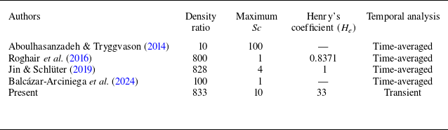

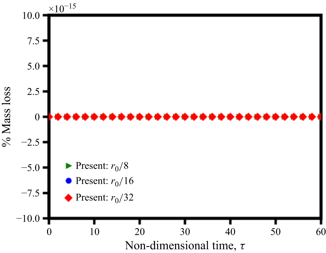
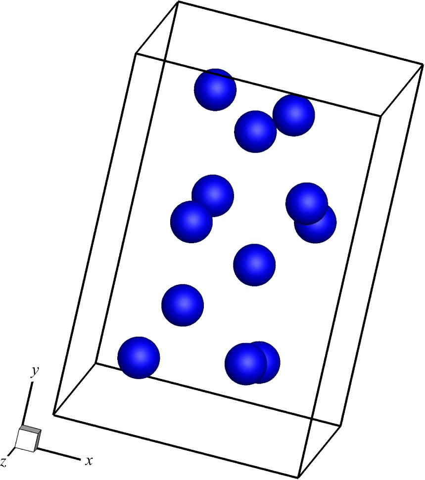


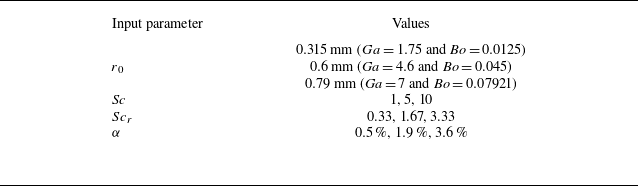


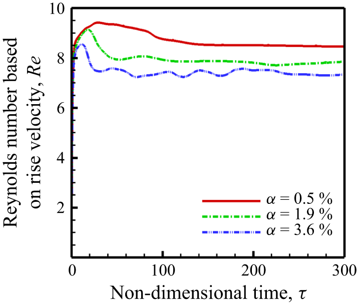


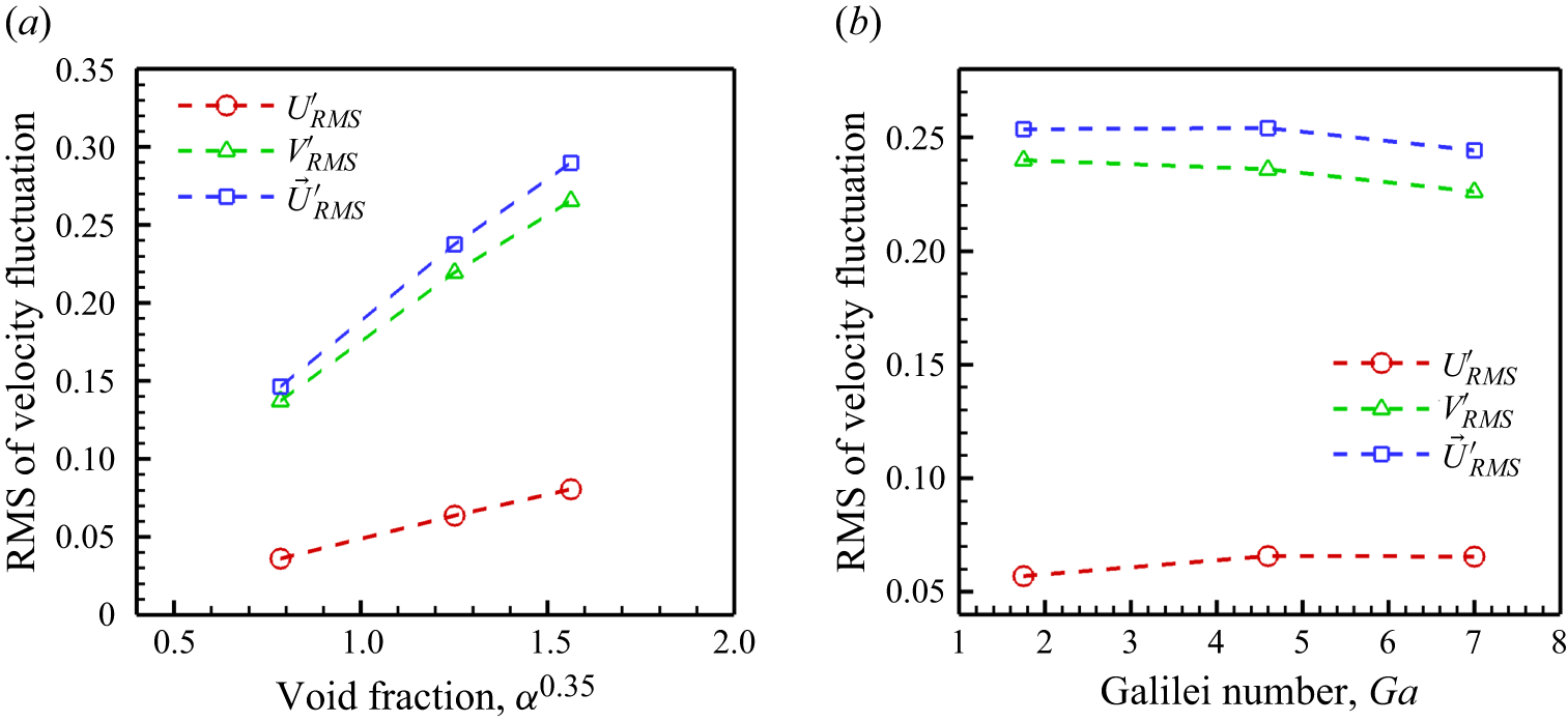


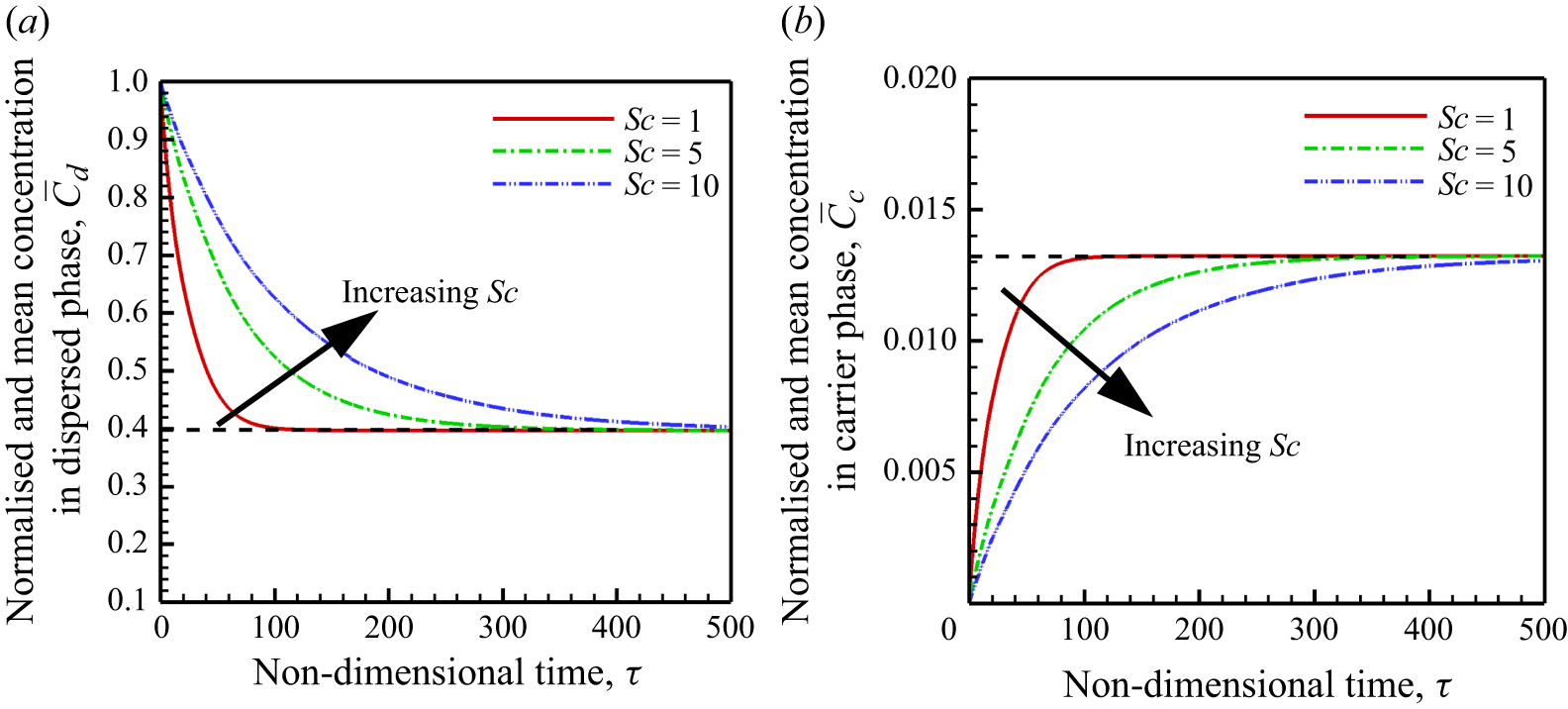


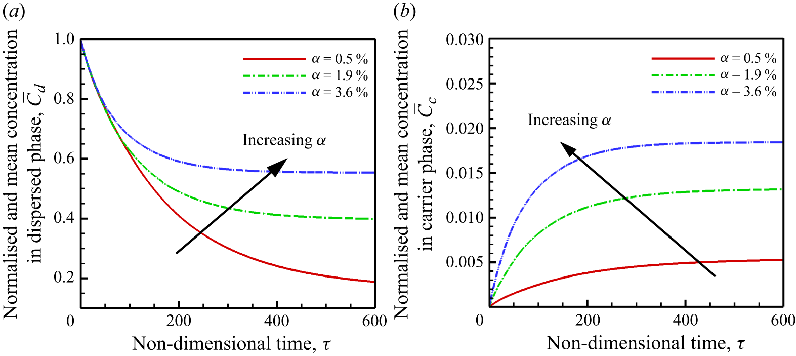


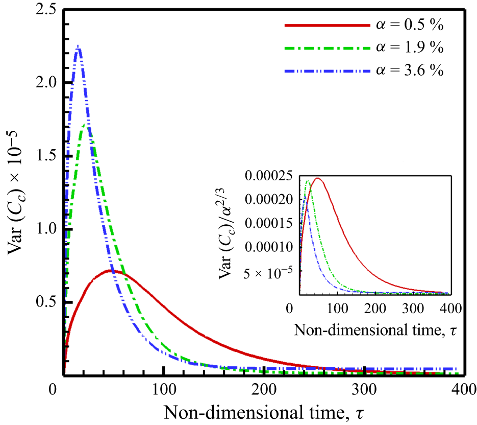


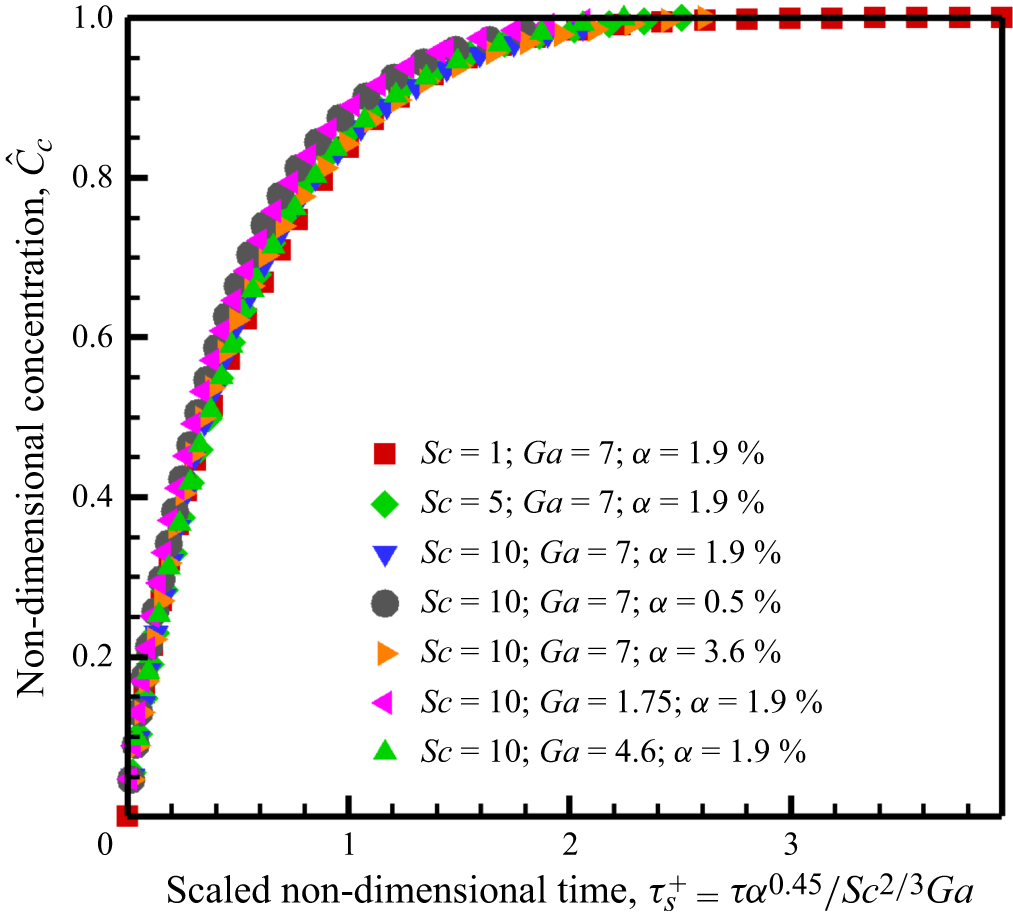


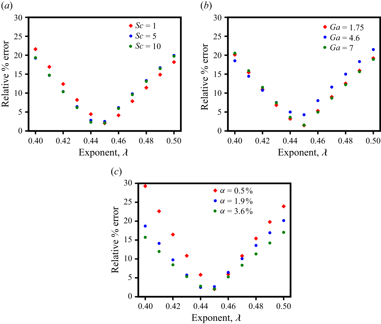


 Open access

