1. Introduction
Inertio-gravity waves are those buoyancy waves in a rotating frame that have the intrinsic wave frequency close to the local rotation frequency
 $f$
so that their properties are influenced by Coriolis effects. Jones (Reference Jones1967) found that monochromatic gravity waves that propagate in a shear flow in a rotating frame have three critical levels: the classical one in which the background flow equals the wave phase speed similar to the one obtained for internal gravity waves, and two extra levels that are located where the magnitude of the intrinsic wave frequency
 $\pm {\it\Omega}$
equals the Coriolis frequency
 $f$
. He found that the critical levels of inertio-gravity waves have different properties from the internal gravity wave critical levels. In particular, a transverse perturbation to the horizontal wind perturbation is induced as the inertio-gravity wave propagates towards its critical levels; indeed, the wave tends to a circular polarization as the wave propagates towards its critical levels. The strong attenuation of internal gravity waves at the critical levels shown by Booker & Bretherton (Reference Booker and Bretherton1967) is also found for inertio-gravity waves (Grimshaw Reference Grimshaw1975).
There is a large amount of observational evidence that shows important peaks of the frequency spectrum in the atmosphere close to the local Coriolis frequency. The early work of Thompson (Reference Thompson1978) examined radiosondes launched in Australia (38° S) and it showed traces of waves with wavelengths between 1 and 3 km with a strong anticyclonic rotation of the wind vector that have their wave energy concentrated near the local inertial frequency. Cadet & Teitelbaum (Reference Cadet and Teitelbaum1979) also detected stratospheric inertial waves from radiosondes launched every 3 h from a ship at 8.5° N and 23° W. A statistical analysis of MU (middle and upper atmosphere) radar data at (35° N, 136° E) over the course of three years showed gravity waves with an average frequency of
 $f/{\it\Omega}\approx 0.5$
in the height range of 16–22 km (Sato Reference Sato1994). Uninterrupted observations with the MU radar over three weeks showed the presence of inertial waves of
 $f/{\it\Omega}\approx 0.8$
at a height of 22 km (Sato, O’Sullivan & Dunkerton Reference Sato, O’Sullivan and Dunkerton1997). Radiosondes launched from an experimental ship in a wide latitudinal range from 28° N to 48° S at intervals of 1° showed that gravity waves of
 $f/{\it\Omega}\approx 0.5$
were localized in the lower stratosphere and waves of
 $f/{\it\Omega}\approx 0.3$
in the troposphere; no latitudinal dependences of the frequency were found (Yamamori & Sato Reference Yamamori and Sato2006). An event of two inertio-gravity waves with
 $f/{\it\Omega}\approx 0.5$
and
 $f/{\it\Omega}\approx 0.8$
was captured by Tateno & Sato (Reference Tateno and Sato2008) in an intensive radiosonde campaign in which high-vertical-resolution radiosondes (10 m vertical resolution) were launched every 3 h. Measurements with superpressure balloons also showed a peak in wave energy near the inertial frequency (Hertzog et al.
Reference Hertzog, Vidal, Mechoso, Basdevant and Coquerez2002). These superpressure balloons follow a quasi-Lagrangian trajectory and thus allow one to measure directly intrinsic frequencies. Therefore, inertio-gravity wave events appear to be ubiquitous in the lower stratosphere, particularly in low latitudes. However, the dominance of inertio-gravity waves in observed vertical profiles may be favoured because low-frequency gravity waves are easier to capture from observations than high-frequency waves (Alexander, Tsuda & Vincent Reference Alexander, Tsuda and Vincent2002).
Although inertio-gravity waves are thought to transport a lower amount of momentum flux from sources to the middle atmosphere than higher-frequency gravity waves, they can connect sources and sinks of wave momentum flux that are horizontally very far apart, an aspect that is largely ignored in the current gravity wave parametrizations implemented in climate and weather forecast models (e.g. Warner & McIntyre Reference Warner and McIntyre1996; Hines Reference Hines1997). Inertio-gravity waves can propagate very long horizontal distances because the ratio between the vertical group velocity and the horizontal group velocity is small compared with that for higher-frequency waves (e.g. Dunkerton Reference Dunkerton1984). In a recent work, Sato et al. (Reference Sato, Tateno, Watanabe and Kawatani2012), using high-resolution numerical simulations of a general circulation model, found that waves with long horizontal wavelength (
 ${\approx}300{-}400\ \text{km}$
) generated by Andes topography over Patagonia and the Antarctic peninsula are propagated several thousands of kilometres from the mountains. Sato et al. argued that these waves are likely to be the main factor that contributes to the global maximum of momentum flux found with satellite data (e.g. Alexander et al.
Reference Alexander, Gille, Cavanaugh, Coffey, Craig, Eden, Francis, Halvorson, Hannigan, Khosravi, Kinnison, Lee, Massie, Nardi, Barnett, Hepplewhite, Lambert and Dean2008, Reference Alexander, Geller, McLandress, Polavarapu, Preusse, Sassi, Sato, Eckermann, Ern, Hertzog, Kawatani, Pulido, Shaw, Sigmond, Vincent and Watanabe2010). Further observational evidence in Patagonia also showed the presence of high-amplitude gravity waves generated from the Andes mountain range with 240 km of zonal wavelength and an intrinsic frequency of
 $f/{\it\Omega}\approx 0.3$
(Pulido et al.
Reference Pulido, Rodas, Dechat and Lucini2013) so that the waves found in the Patagonia region and the Antarctic peninsula propagate very long distances and are affected significantly by rotation effects. Apart from orographic forcing, other significant sources of inertio-gravity waves are fronts and jets in middle latitudes (O’Sullivan & Dunkerton Reference O’Sullivan and Dunkerton1995; Zhang Reference Zhang2004) and deep convection in the tropics (Lane, Reeder & Clark Reference Lane, Reeder and Clark2001). Furthermore, simulations of moist jet-front systems, which combine two possible sources, jet and convection, show gravity waves with higher amplitudes than in dry simulations (Wei & Zhang Reference Wei and Zhang2014).
A further distinctive aspect of inertio-gravity waves that propagate in shear flows is the characteristics of the wave breaking. The wave breaking characteristics determine the wave momentum flux deposition in the background flow, i.e. the distribution of the wave momentum flux divergences, which is relevant for the parametrizations of unresolved gravity waves in climate and weather forecast models. Fritts & Rastogi (Reference Fritts and Rastogi1985) showed that inertio-gravity waves with frequency close to the Coriolis frequency can reach the amplitude threshold for the dynamical instability at lower heights than the convective instability threshold. This result is contrary to what was found for internal gravity waves (Hodges Reference Hodges1967). Fritts & Yuan (Reference Fritts and Yuan1989) used a linear stability analysis to examine the conditions for which inertio-gravity waves produce a Kelvin–Helmholtz instability in a flow without shear. They found that the instability has a faster growth rate in the transverse direction to the wave propagation direction when the frequency of the wave is close to the Coriolis frequency. Yuan & Fritts (Reference Yuan and Fritts1989) extended the previous work for inertio-gravity waves in a shear flow; the dynamical instabilities are found for a wider range of frequencies and they have faster growth rates when the waves propagate in a shear flow. Dunkerton (Reference Dunkerton1997) further extended the linear stability analysis for a situation in which the inertio-gravity wave propagates in a background flow that resembles a gravity wavepacket without mean shear. He showed that the dynamical instability is the dominant mechanism for
 $f/{\it\Omega}\rightarrow 1$
, while for
 $f/{\it\Omega}\rightarrow 0$
the convective instability is dominant. For intermediate values of
 $f/{\it\Omega}$
, a hybrid convective–dynamical instability is expected. Numerical simulations of the three-dimensional breaking of an inertio-gravity wave with intrinsic frequency close to the inertial frequency confirm that the wave breaks preferentially through dynamical instability (Lelong & Dunkerton Reference Lelong and Dunkerton1998a
), even when the convective instability is established initially by the wave (Lelong & Dunkerton Reference Lelong and Dunkerton1998b
).
In this work, we examine the propagation and breaking mechanism of transient inertio-gravity waves in a shear flow. Previous works assume a steady-state wave field, so that the inertio-gravity wave has a fixed frequency, which produces three critical levels in a shear flow. In the case of a transient wave in a shear flow, there is a continuous frequency spectrum associated with the wave so that the different components of the frequency spectrum reach critical levels at different heights.
Pulido & Rodas (Reference Pulido and Rodas2008) examined a transient internal gravity wave that propagates in a shear flow (in a system without rotation) towards the critical level. They found that the wave amplitude of the horizontal wind reaches a maximum and then decays asymptotically as the inverse root square of time, contrary to steady-state waves (i.e. monochromatic waves) whose amplitude becomes unbounded at the critical level. Two extreme breaking regimes are found. On the one hand, quasi-monochromatic waves with a large initial amplitude break with amplitude and height close to those of the monochromatic wave (before the waves reach the maximum amplitude), keeping the classical image of wave overturning. On the other hand, highly transient wavepackets break very close to the critical level with small amplitudes and high vertical wavenumber so that dissipative effects are likely to be important in this regime.
To determine the wave amplitude and height of the breaking for transient waves, the usual spatial ray theory (Lighthill Reference Lighthill1978) is not useful, and nor are the stationary phase methods, because they only give the asymptotic tendency for long times, while transient waves may reach the instability threshold before attaining the asymptotic regime. Indeed, transient gravity wavepackets reach the maximum amplitude during propagation well below the critical level, a feature that is not captured with the first-order asymptotic approaches (Pulido & Rodas Reference Pulido and Rodas2008). The Gaussian beam formulation, which is extensively used in other contexts such as optics (Heyman & Felsen Reference Heyman and Felsen2001), quantum mechanics (Hagedorn Reference Hagedorn1984) and seismic waves (Cerveny, Popov & Psencik Reference Cerveny, Popov and Psencik1982; Cerveny Reference Cerveny1983), is able to represent the wavepacket from the early times – this formulation is free of the caustic artifacts that appear in the spatial ray path, in particular at the initial time – up to long times when it reaches the asymptotic behaviour. Therefore, the Gaussian beam formulation is a very useful technique to determine the characteristics of gravity wave propagation as a function of the wave and background flow parameters.
One of the reasons that turned our attention to study inertial effects using the Gaussian beam formulation is that waves of any absolute frequency, as long as they propagate in a geophysical flow towards the critical level, will have an intrinsic frequency that tend towards the Coriolis frequency and therefore any gravity wave is affected by inertial effects in the neighbourhood of the critical level. This effect is expected to be particularly important for transient waves that have a critical height range. Our main purpose is thus to determine the characteristics of the breaking of transient inertio-gravity waves as a function of the main parameters of the wave and the background system using the Gaussian beam formulation.
The work is organized as follows. In § 2, the Wentzel–Kramers–Brillouin–Jeffreys (WKBJ) solution of an inertio-gravity wave in a shear flow is given, and then it is used in a frequency spectrum to derive the Gaussian beam formulation. The main characteristics of transient inertio-gravity waves propagating in a shear flow are examined. Section 3 introduces an analysis of the possible instabilities that induce the inertio-gravity waves as they propagate towards critical levels. Numerical simulations and their comparisons with the Gaussian beam formulation are given in § 2.2. Finally we draw the conclusions of the work in § 4.
2. Mathematical formulation
Consider small adiabatic buoyancy perturbations under the effect of gravity
 $g$
in a background flow that is time-independent and horizontally uniform so that the only dependence of the background flow is on height, i.e.
 $u_{0}(z)$
. The coordinate frame rotates with an angular frequency
 $f$
. The hydrostatic and inviscid approximations are taken for the derivation. Since the coefficients of the equations are independent of
 $x$
,
 $y$
and
 $t$
, we propose a harmonic solution for the vertical velocity perturbation of the form
 $$\begin{eqnarray}w_{1}(x,y,z,t)=\tilde{w}(z)\exp [\text{i}({\it\omega}t-kx-ly)],\end{eqnarray}$$
where
 ${\it\omega}$
is the absolute frequency, and
 $k$
and
 $l$
are the wavenumbers in the
 $x$
and
 $y$
directions, respectively. To simplify the presentation in what follows, we assume a wave with null wavenumber in
 $y$
,
 $l=0$
. The generalization is straightforward and it does not add any qualitative effect.
Replacing (2.1) in the equations, an ordinary differential equation is obtained for
 $\tilde{w}(z)$
(Jones Reference Jones1967),
 $$\begin{eqnarray}\frac{\text{d}^{2}\tilde{w}}{\text{d}z^{2}}-\left[\frac{2k\,f^{2}d_{z}u_{0}}{{\it\Omega}({\it\Omega}^{2}-f^{2})}\right]\frac{\text{d}\tilde{w}}{\text{d}z}+\left(\frac{N_{0}^{2}k^{2}}{{\it\Omega}^{2}-f^{2}}\right)\tilde{w}=0,\end{eqnarray}$$
where
 ${\it\Omega}={\it\omega}-ku_{0}$
is the intrinsic frequency,
 $N_{0}$
is the constant buoyancy frequency, also known as the Brunt–Väisälä frequency, and
 $d_{z}u_{0}$
is the background shear. The background flow curvature,
 $\text{d}^{2}u_{0}/\text{d}z^{2}$
, is considered negligible.
2.1. Wentzel–Kramers–Brillouin–Jeffreys approximation
An approximated solution to (2.2) may be found using the well-known WKBJ method (Bender & Orszag Reference Bender and Orszag1978) following the works of Wentzel, Kramers, Brillouin and Jeffreys. This is an asymptotic method that approximates ordinary differential equations with coefficients that vary with the independent variable. A solution of the form
 $$\begin{eqnarray}\tilde{w}(z)\approx \exp \left[\frac{1}{{\it\epsilon}}\mathop{\sum }\limits_{n=0}^{\infty }{\it\epsilon}^{n}S_{n}(z)\right]\end{eqnarray}$$
is proposed, where
 ${\it\epsilon}$
is the smallness parameter of the asymptotic series. The dependences with the smallness parameter are made explicit in (2.3) in this way;
 $S_{n}(z)$
is assumed to be of order one (
 $S_{n}(z)$
does not depend on the
 ${\it\epsilon}$
parameter). The independent variable
 $z$
is also assumed to be of order one. A set of differential equations for
 $S_{n}$
is obtained by replacing (2.3) in (2.2) for the different powers of
 ${\it\epsilon}$
.
The first two equations, which correspond to the two lowest orders in
 ${\it\epsilon}$
, are obtained by replacing (2.3) in (2.2) and identifying the orders
 ${\it\epsilon}^{-2}$
and
 ${\it\epsilon}^{-1}$
in the resulting equation. They are, respectively,
 $$\begin{eqnarray}\displaystyle & \displaystyle \frac{1}{{\it\epsilon}^{2}}\left[\frac{\text{d}S_{0}(z)}{\text{d}z}\right]^{2}+\frac{N_{0}^{2}k^{2}}{{\it\Omega}^{2}-f^{2}}=0, & \displaystyle\end{eqnarray}$$
 $$\begin{eqnarray}\displaystyle & \displaystyle 2\frac{\text{d}S_{0}(z)}{\text{d}z}\,\frac{\text{d}S_{1}(z)}{\text{d}z}-\frac{2k\,f^{2}d_{z}u_{0}}{{\it\Omega}({\it\Omega}^{2}-f^{2})}\frac{\text{d}S_{0}(z)}{\text{d}z}+\frac{\text{d}^{2}S_{0}(z)}{\text{d}z^{2}}=0, & \displaystyle\end{eqnarray}$$
 $N_{0}^{2}k^{2}/({\it\Omega}^{2}-f^{2})$
is of order
 ${\it\epsilon}^{-2}$
.
The proposed solution (2.3) must satisfy approximately the differential equation (2.2). If we replace (2.3) up to order
 $n=1$
in (2.2), the WKBJ solution satisfies exactly
 $$\begin{eqnarray}\displaystyle & & \displaystyle \left\{\left[\frac{1}{{\it\epsilon}}\frac{\text{d}^{2}S_{0}}{\text{d}z^{2}}+\frac{\text{d}^{2}S_{1}}{\text{d}z^{2}}+\left(\frac{1}{{\it\epsilon}}\frac{\text{d}S_{0}}{\text{d}z}+\frac{\text{d}S_{1}}{\text{d}z}\right)^{2}\right]\right.\nonumber\\ \displaystyle & & \displaystyle \quad \left.-\left[\frac{2k\,f^{2}d_{z}u_{0}}{{\it\Omega}({\it\Omega}^{2}-f^{2})}\right]\left(\frac{1}{{\it\epsilon}}\frac{\text{d}S_{0}}{\text{d}z}+\frac{\text{d}S_{1}}{\text{d}z}\right)+\left(\frac{N_{0}^{2}k^{2}}{{\it\Omega}^{2}-f^{2}}\right)[1+d(z)]\right\}\tilde{w}=0,\end{eqnarray}$$
where we represent explicitly the error of the WKBJ solution,
 $d(z)$
, in satisfying the exact differential equation (2.2). If
 $d(z)=0$
, the WKBJ solution (2.3), up to
 $n=1$
, would be an exact solution of (2.2). If
 $d(z)$
is small (
 $|d(z)|\ll 1$
), the WKBJ solution is an approximate solution of (2.2).
The solution of (2.4)–(2.5) is
 $$\begin{eqnarray}S_{0}(z)=\pm \text{i}{\it\epsilon}\int _{z_{i}}^{z}\left[\frac{N_{0}k}{({\it\Omega}^{2}-f^{2})^{1/2}}\right]\text{d}z^{\prime }\end{eqnarray}$$
and
 $$\begin{eqnarray}S_{1}(z)=\int _{z_{i}}^{z}\frac{k\,f^{2}d_{z}u_{0}}{{\it\Omega}({\it\Omega}^{2}-f^{2})}\,\text{d}z^{\prime }-\frac{1}{4}\ln \left(\frac{{\it\Omega}_{i}^{2}-f^{2}}{{\it\Omega}^{2}-f^{2}}\right),\end{eqnarray}$$
where
 $z_{i}$
is taken as the reference height and
 ${\it\Omega}_{i}={\it\omega}-ku_{0}(z_{i})$
is the intrinsic frequency at the reference height.
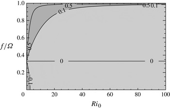
The smallness WKBJ parameter
 $d$
as a function of
 $\mathit{Ri}_{0}$
and
 $f/{\it\Omega}$
. The curves for
 $d=[-0.1,0,0.1,0.5]$
are shown. The lighter grey shaded region represents
 $|d|<0.1$
for which the WKBJ approximation is considered valid.

Therefore, replacing (2.7) and (2.8) in (2.3) we obtain the WKBJ solution of (2.2),
 $$\begin{eqnarray}\tilde{w}(z)={\hat{w}}\left(\frac{{\it\Omega}_{i}^{2}-f^{2}}{{\it\Omega}^{2}-f^{2}}\right)^{1/4}\left(\frac{{\it\Omega}}{{\it\Omega}_{i}}\right)\exp \left\{\pm \text{i}\int _{z_{i}}^{z}\frac{N_{0}k}{({\it\Omega}^{2}-f^{2})^{1/2}}\,\text{d}z^{\prime }\right\},\end{eqnarray}$$
where
 ${\hat{w}}$
is the wave amplitude at the reference height and hereinafter we leave the smallness parameter implicit. The derivative of the imaginary exponent can be identified as the local vertical wavenumber
 $m$
at
 $z$
, and thus the local dispersion relation is
 $$\begin{eqnarray}m=\pm \frac{N_{0}k}{({\it\Omega}^{2}-f^{2})^{1/2}}.\end{eqnarray}$$
The signs in (2.10) represent upward and downward propagation. For
 $k>0$
, the negative sign in (2.10) indicates upward propagation of the waves.
The range of validity of the WKBJ approximation is obtained by replacing (2.7) and (2.8) in (2.6). The WKBJ solution, (2.9), is a good approximation as long as
 $$\begin{eqnarray}d(z)=\frac{1}{\mathit{Ri}_{0}(1-f^{2}/{\it\Omega}^{2})}\left|\frac{1}{4}-\frac{5}{2}\frac{f^{2}}{{\it\Omega}^{2}}+2\frac{f^{4}}{{\it\Omega}^{4}}\right|\ll 1.\end{eqnarray}$$
The smallness parameter
 $d$
as a function of the background Richardson number,
 $\mathit{Ri}_{0}=N_{0}^{2}/(d_{z}u_{0})^{2}$
, and
 $f/{\it\Omega}$
is shown in figure 1. The lighter grey shaded region in figure 1 represents
 $|d|\ll 1$
in which the WKBJ solution (2.9) is expected to be a good approximation. For
 $\mathit{Ri}_{0}=40$
, the approximation is valid for
 $f/{\it\Omega}\lessapprox 0.95$
and for
 $\mathit{Ri}_{0}=80$
the validity of the approximation is extended up to
 $f/{\it\Omega}\lessapprox 0.98$
. For
 $f/{\it\Omega}\rightarrow 0$
, the approximation from (2.11) is valid in general for large
 $\mathit{Ri}_{0}$
, which is the known limit of validity of the WKBJ approximation for internal gravity waves (e.g. Pulido & Rodas Reference Pulido and Rodas2011). For
 $f/{\it\Omega}={\textstyle \frac{1}{2}}({\textstyle \frac{5}{2}}-{\textstyle \frac{1}{2}}\sqrt{17})^{1/2}\approx 0.33$
, the expression between bars in (2.11) is zero, so that
 $d$
is small for
 $f/{\it\Omega}$
close to 0.33 independently of the Richardson number value. In this case, the WKBJ approximation holds even for small Richardson numbers.
Since the velocity field is divergence-free,
 ${\hat{u}}=k^{-1}m{\hat{w}}$
, using (2.9) the horizontal velocity perturbation in
 $x$
is
 $$\begin{eqnarray}{\tilde{u}}(z)={\hat{u}}\left(\frac{{\it\Omega}_{i}^{2}-f^{2}}{{\it\Omega}^{2}-f^{2}}\right)^{3/4}\left(\frac{{\it\Omega}}{{\it\Omega}_{i}}\right)\exp \left\{\pm \text{i}\int _{0}^{z}\frac{N_{0}k}{({\it\Omega}^{2}-f^{2})^{1/2}}\,\text{d}z^{\prime }\right\}.\end{eqnarray}$$
The wave energy density is given by the sum of the kinetic and potential wave energy,
 $$\begin{eqnarray}W_{r}={\textstyle \frac{1}{2}}{\it\rho}_{0}\left(\overline{u_{1}^{2}}+\overline{v_{1}^{2}}+N_{0}^{2}\overline{{\it\eta}_{1}^{2}}\right)\!,\end{eqnarray}$$
where
 $v_{1}$
is the component of the velocity perturbation in the
 $y$
direction,
 ${\it\eta}_{1}$
is the vertical displacement produced by the perturbation and the overlines represent an average in phase. Because the hydrostatic approximation is taken since we consider low-frequency waves, the vertical velocity contribution to the kinetic energy is negligible. Even when
 $l$
is assumed zero, the component
 $v_{1}$
is not null from the polarization relationship; indeed, inertio-gravity waves have an elliptical polarization.
The wave energy is not equipartitioned between kinetic and potential energy for inertio-gravity waves (e.g. Gill Reference Gill1982) contrary to internal gravity waves. As the intrinsic frequency goes to the Coriolis frequency, the kinetic energy increases and the potential energy decreases.
Using the polarization relations for inertio-gravity waves and considering
 $N_{0}^{2}\gg {\it\Omega}^{2}$
in (2.13), we obtain
 $$\begin{eqnarray}W_{r}=\frac{1}{2}{\it\rho}_{0}\,\overline{u_{1}^{2}}\left[1+\frac{1}{{\it\Omega}^{2}}\left(f^{2}+\frac{N_{0}^{2}k^{2}}{m^{2}}\right)\right]\!.\end{eqnarray}$$
 $$\begin{eqnarray}W_{r}={\it\rho}_{0}\,\overline{u_{1}^{2}}.\end{eqnarray}$$
Note that (2.15) is similar to the expression for the wave energy density obtained in Pulido & Rodas (Reference Pulido and Rodas2008) for internal gravity waves, but in that case the derivation is based on energy equipartition while for inertio-gravity waves that principle is not valid.
2.2. Gaussian beam formulation
The general solution for transient inertio-gravity waves can be expressed as a linear superposition in frequency of the harmonic solution (2.12),
 $$\begin{eqnarray}u_{1}(x,z,t)=\frac{1}{\sqrt{2{\rm\pi}}}\int _{-\infty }^{\infty }{\hat{u}}({\it\omega})\left(\frac{{\it\Omega}({\it\omega},z_{i})^{2}-f^{2}}{{\it\Omega}({\it\omega},z)^{2}-f^{2}}\right)^{3/4}\frac{{\it\Omega}({\it\omega},z)}{{\it\Omega}({\it\omega},z_{i})}\exp (\text{i}{\it\psi})\text{d}{\it\omega},\end{eqnarray}$$
where the phase is given by
 $$\begin{eqnarray}{\it\psi}={\it\omega}t-kx-\int _{z_{i}}^{z}m({\it\omega},z^{\prime })\text{d}z^{\prime }.\end{eqnarray}$$
To obtain an analytical expression of the solution (2.16), we assume that the wave trains have a frequency distribution concentrated around a dominant frequency, such that the envelope amplitude of the wavepacket changes slowly in a period. For such wavepackets, an asymptotic expansion based on ray theory is a representative approximation of (2.16). The Gaussian beam approximation assumes that the wavepacket propagates concentrated along the ray trajectory and the amplitude of the wavepacket satisfies the Schrödinger equation (Ostrovsky & Potapov Reference Ostrovsky and Potapov1999). The solution of the Schrödinger equation decays exponentially as the square of the distance to the ray. This gives the name to the approximation (Cerveny Reference Cerveny1983). Therefore, the approximation associates with each ray a beam or tube that has a Gaussian section normal to the ray.
Here, we apply the approximation directly in the frequency space. A Gaussian frequency spectrum relatively concentrated around a central frequency
 ${\it\omega}_{c}$
of frequency width
 ${\it\sigma}_{{\it\omega}}$
is proposed,
 $$\begin{eqnarray}{\hat{u}}({\it\omega})=\frac{{\hat{u}}_{{\it\omega}}}{{\it\sigma}_{{\it\omega}}}\exp \left[-\frac{({\it\omega}-{\it\omega}_{c})^{2}}{2{\it\sigma}_{{\it\omega}}^{2}}\right].\end{eqnarray}$$
As the spectrum is assumed to be concentrated, we expand the phase in a Taylor series up to second order in
 ${\it\omega}$
around
 ${\it\omega}_{c}$
. The first term in the Taylor series of the amplitude is the only one that we keep in the amplitude expansion. The changes in the amplitude term are assumed to be slower than the changes in the oscillatory term. This is also consistent with the WKBJ approximation (2.3) and it is valid for
 $d\ll 1$
(see (2.11)).
A detailed derivation of the Gaussian beam approximation for mountain waves may be found in Pulido & Rodas (Reference Pulido and Rodas2011). A formal proof for mountain waves that shows that the equation system is well posed and the Gaussian beam approximation is close to the integral solution, (2.16), is given in Tanushev, Quian & Ralston (Reference Tanushev, Quian and Ralston2007). The resulting wave perturbation after replacing (2.18) in (2.16) and integrating (2.16) by completing squares (see Pulido & Rodas Reference Pulido and Rodas2011) is
 $$\begin{eqnarray}\displaystyle u_{1} & = & \displaystyle \frac{{\hat{u}}_{{\it\omega}}}{{\it\sigma}_{{\it\omega}}}\left(\frac{{\it\Omega}_{ic}^{2}-f^{2}}{{\it\Omega}_{c}^{2}-f^{2}}\right)^{3/4}\frac{{\it\Omega}_{c}}{{\it\Omega}_{ic}}\,\frac{\exp \{\text{i}[{\it\psi}_{c}-\tan ^{-1}(-\partial _{{\it\omega}{\it\omega}}^{2}{\it\psi}_{c}{\it\sigma}_{{\it\omega}}^{2})/2]\}}{\left[1/{\it\sigma}_{{\it\omega}}^{4}+(\partial _{{\it\omega}{\it\omega}}^{2}{\it\psi}_{c})^{2}\right]^{1/4}}\nonumber\\ \displaystyle & & \displaystyle \times \exp \left[-\frac{(\partial _{{\it\omega}}{\it\psi}_{c})^{2}}{2({\it\sigma}_{{\it\omega}}^{-2}-\text{i}\partial _{{\it\omega}{\it\omega}}^{2}{\it\psi}_{c})}\right],\end{eqnarray}$$
 $c$
subindex represents evaluation at the central absolute frequency,
 ${\it\Omega}_{c}$
is the central intrinsic frequency and
 ${\it\Omega}_{ic}$
is the initial central intrinsic frequency. The transient inertio-gravity wave solution obtained in (2.19) differs from the solution obtained by Pulido & Rodas (Reference Pulido and Rodas2008) for transient internal waves in the amplitude and phase terms due to the dispersion relation.
The part of the exponential with imaginary argument in (2.19) represents the phase that defines the central ray given by the stationary phase points
 $$\begin{eqnarray}\partial _{{\it\omega}}{\it\psi}_{c}=0.\end{eqnarray}$$
The Gaussian beam approximation removes one of the main limitations of spatial ray tracing, which predicts a singularity in the points where rays intersect between them, called caustics. This includes the initial time of transient wavepackets and a vertical line above the mountain, for mountain waves which indeed is the location of the maximum wave amplitude (e.g. Pulido & Rodas Reference Pulido and Rodas2011). The Gaussian beam approximation considers not only the central ray but a bunch of rays around the central one, so that it accounts not only for the convergence and divergence of rays (as the spatial ray path does) but also for the interference between neighbouring rays.
2.3. Evolution of the wave amplitude
The amplitude of the disturbance is defined by
 $A(z,t)=\sqrt{\bar{u_{1}^{2}}}$
. This represents the envelope amplitude and the square of it is the wave energy per unit mass, i.e.
 $W_{r}/{\it\rho}=A^{2}$
. From (2.19), the evolution of
 $A$
is given by
 $$\begin{eqnarray}\displaystyle A(z,t) & = & \displaystyle {\hat{u}}_{{\it\omega}}\left(\frac{{\it\Omega}_{ic}^{2}-f^{2}}{{\it\Omega}_{c}^{2}-f^{2}}\right)^{3/4}\frac{{\it\Omega}_{c}}{{\it\Omega}_{ic}}[1+{\it\sigma}_{{\it\omega}}^{4}(\partial _{{\it\omega}{\it\omega}}^{2}{\it\psi}_{c})^{2}]^{-1/4}\nonumber\\ \displaystyle & & \displaystyle \times \exp \left\{-\frac{(\partial _{{\it\omega}}{\it\psi}_{c})^{2}}{2[{\it\sigma}_{{\it\omega}}^{-2}+({\it\sigma}_{{\it\omega}}\partial _{{\it\omega}{\it\omega}}^{2}{\it\psi}_{c})^{2}]}\right\}.\end{eqnarray}$$
Equation (2.21) gives the evolution of the wave envelope close to the stationary phase points in
 $z$
as a function of time. The envelope amplitude depends on the second derivative of the phase, which represents the dispersion of the wavepacket, i.e. the amplitude diminishes with time because trajectories of the rays with different absolute frequency separate. The exponential in (2.21) gives the amplitude of the beam around the central ray path determined by (2.20).
We are interested in the maximum amplitude of the wave envelope, because this point will first reach the wave overturning threshold. The maximum wave amplitude is located along the central ray path, so that evaluating
 $z$
in (2.21) at the altitude of the central ray for each time (say
 $z_{c}(t)$
, which is determined from (2.20)) gives the maximum amplitude of the wave envelope as a function of time,
 $$\begin{eqnarray}a(t)={\hat{u}}_{{\it\omega}}\left(\frac{{\it\Omega}_{ic}^{2}-f^{2}}{{\it\Omega}_{c}^{2}-f^{2}}\right)^{3/4}\frac{{\it\Omega}_{c}}{{\it\Omega}_{ic}}\,[1+{\it\sigma}_{{\it\omega}}^{4}(\partial _{{\it\omega}{\it\omega}}^{2}{\it\psi}_{c})^{2}]^{-1/4},\end{eqnarray}$$
where
 ${\it\Omega}_{c}$
and
 $\partial _{{\it\omega}{\it\omega}}^{2}{\it\psi}_{c}$
must be evaluated at (2.20).
At the initial time,
 $\partial _{{\it\omega}{\it\omega}}^{2}{\it\psi}_{c}(t=0)=0$
, so that from (2.22)
 $a(0)={\hat{u}}_{{\it\omega}}$
. The Gaussian beam approximation is a good approximation of the disturbance for any time. There are also some techniques based on spatial ray tracing that give a finite amplitude at any time. For instance, the first formulation proposed by Hayes (Reference Hayes1970), who suggests solving an extra differential equation for the gradient of the wavenumber vector (so that the gradient of the wavenumber vector must be specified at the lower boundary). Broutman, Rottman & Eckermann (Reference Broutman, Rottman and Eckermann2001) propose solving an integral representation of the wave field close to the source and then to use ray tracing in the far field.
3. Results
The Gaussian beam approximation introduced in the previous section is now applied to examine the breaking conditions of transient inertio-gravity waves that propagate in a shear flow towards the critical level. The results of the Gaussian beam approximation are contrasted with an exact linear numerical model. The numerical model does not pretend to be realistic, but to evaluate the limitations of the Gaussian beam approximation in a linear context.
The numerical simulations were conducted with the numerical model introduced in Pulido (Reference Pulido2005). It models the propagation of gravity waves in shear flows by solving the Taylor–Goldstein equation in the spectral space for each spectral component. The Taylor–Goldstein equation is solved by transforming it to two first-order differential equations, which are solved using the fourth-order Runge–Kutta scheme with adaptive step size (Press et al.
Reference Press, Flannery, Teukolsky and Vetterling1992). For the numerical experiments in this work, the Taylor–Goldstein equation that we solve is (2.2). Finally, spectral components that are the solution of the Taylor–Goldstein equation are Fourier-transformed to the physical space. The amplitude of spectral components which are given approximately by (2.12) goes as
 $({\it\Omega}^{2}-f^{2})^{-3/4}$
so that it is infinite at the critical levels of the component, i.e.
 ${\it\omega}/k-u_{0}(z)\mp f/k=0$
. Each spectral component has a different critical level, so that there is a height range with critical levels, which we call the critical region. However, destructive interference between the components in the general solution (2.16) leads to a finite amplitude at the critical region for the transient inertio-gravity wave. Thus, the numerical model requires very high resolution in both the physical and spectral spaces to give a good approximation close to the critical levels where strong destructive interference between spectral components occurs. The standard number of points that we use in the vertical is 20 000, which gives a height resolution of about
 ${\rm\Delta}z=2\ \text{m}$
, and also 20 000 points in the spectral space centred around the central absolute frequency
 ${\it\omega}_{c}$
. The main computational cost of solving numerically the full integral representation (2.16) is because of this required high spatial and spectral resolution. The computation involves solving the Taylor–Goldstein equation (2.2) (or evaluating the WKBJ solution, (2.12)) in height with a high vertical resolution for each of the 20 000 spectral components, which are then superposed to give (2.16).
The Gaussian beam solution gives directly the wave field in the physical space, (2.19). The computation involves a single evaluation of the function (2.19) in the vertical. Because the interference effects do not need to be represented in this case, only a relatively low vertical resolution is enough. The output of the numerical model is then compared with the wave field of the Gaussian beam approximation. We first show the propagation of wavepackets in a linear background flow for which the Gaussian beam approximation gives analytical results. In this context, the dependences with all the parameters of the wave field and the background flow can be obtained analytically. The application of the Gaussian beam approximation in a realistic environment is shown in § 3.5; for this case a straightforward numerical height integration is required.
3.1. Evolution of the wave amplitude in a flow with constant shear
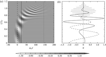
Figure 2(a) shows the zonal velocity perturbation evolution of an inertial wavepacket with central frequency
 ${\it\omega}_{c}=0.10N_{0}$
and spectral width
 ${\it\sigma}_{{\it\omega}}=0.15{\it\omega}_{c}$
that propagates in a background flow with
 $\mathit{Ri}_{0}=100$
and
 $\tilde{f}=f/{\it\omega}_{c}=0.05$
. The reference height is taken as
 $z_{i}=0$
; this is the height at which the wavepacket is launched initially. The height of the central critical level of an internal gravity wavepacket is given by
 $z_{cl}={\it\omega}_{c}/(kd_{z}U)$
. In what follows the vertical coordinate is non-dimensionalized as
 $\tilde{z}=z/z_{cl}$
, so that the critical level height of the internal gravity wavepacket is
 $\tilde{z}_{cl}=1$
. The lowest central inertial critical level will be at a height slightly lower than
 $z_{cl}$
,
 $({\it\omega}_{c}-f)/(kd_{z}U)=0.95z_{cl}$
. The critical region, where each (non-negligible) spectral component (2.12) has its own critical level, goes from
 $z=({\it\omega}_{c}-{\it\sigma}_{{\it\omega}}-f)/(kd_{z}U)=0.8z_{cl}$
up to
 $z=({\it\omega}_{c}+{\it\sigma}_{{\it\omega}}-f)/(k\text{d}_{z}U)=1.1z_{cl}$
.
(a) Zonal velocity perturbation evolution of an inertial gravity wavepacket. Vertical straight lines represent
 ${\it\omega}_{c}t=0$
(dashed),
 ${\it\omega}_{c}t=21.6$
(solid) and
 ${\it\omega}_{c}t=144$
(dotted). (b) Vertical profiles of the zonal perturbation at
 ${\it\omega}_{c}t=0$
(dashed),
 ${\it\omega}_{c}t=21.6$
(solid) and
 ${\it\omega}_{c}t=144$
(dotted). The wavepacket width is
 ${\it\sigma}=0.1{\it\omega}_{c}$
; the background flow is characterized by
 $\mathit{Ri}_{0}=100$
.

The packet propagates upwards with large vertical group velocity at short times; then the vertical group velocity goes to zero as the packet gets closer to the central critical level. As the wavepacket propagates towards the central critical level, the central vertical wavenumber of the packet increases because of Doppler shifting. The vertical width of the wavepacket is broad at the initial time, then reaches a minimum at about
 ${\it\omega}_{c}t=100.8$
and finally goes to an asymptotic constant value for long times (
 ${\it\omega}_{c}t\gg 100$
). The amplitude of the wavepacket increases at short times, it achieves a maximum and then at long times it decreases asymptotically towards a constant (see also the evolution of the wavepacket envelope amplitude in figure 3
a). The evolution of the wavepacket envelope amplitude is discussed below. Figure 2(b) shows the vertical profile of the zonal velocity perturbation at the initial time, at the time of maximum amplitude (
 ${\it\omega}_{c}t=21.6$
) and when the packet is close to the asymptotic behaviour (
 ${\it\omega}_{c}t=144$
). The amplitude, width and vertical wavenumber dependences already mentioned are clearly identified in these profiles. Note that, as the packet gets closer to the critical level, the envelope is composed by several vertical wavelengths, which is the assumption of both ray tracing and Gaussian beam approximations.
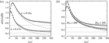
Amplitude evolution of an inertial wavepacket. (a) Wavepacket widths of
 ${\it\sigma}=0.1{\it\omega}_{c}$
and
 ${\it\sigma}=0.17{\it\omega}_{c}$
and
 $\mathit{Ri}_{0}=100$
. (b) Background flow characterized by
 $\mathit{Ri}_{0}=100$
and
 $\mathit{Ri}_{0}=400$
and a wavepacket width of
 ${\it\sigma}=0.1{\it\omega}_{c}$
. For each case, three curves are shown: Gaussian beam approximation for inertial waves (solid), Gaussian beam approximation for internal waves (dashed) and the numerical integration for inertial waves (triangles). The asymptotic values for inertial waves are shown with dotted straight lines.

The analytical calculations for the Gaussian beam approximation are conducted for a background flow with constant vertical shear,
 $\text{d}u_{0}/\text{d}z={\it\Gamma}$
. The evolution of the maximum amplitude of the wave envelope under the Gaussian beam approximation in a flow with constant shear using (2.22) is
 $$\begin{eqnarray}a(t)={\hat{u}}_{{\it\omega}}\frac{(1+{\it\gamma}_{c}\mathit{Ri}_{0}^{-1/2}t)^{1/2}[{\it\gamma}_{c}^{2}+f^{2}(1+{\it\gamma}_{c}\mathit{Ri}_{0}^{-1/2}t)^{2}]^{1/2}}{{\it\omega}_{c}\left\{1+{\it\sigma}_{{\it\omega}}^{4}\,\displaystyle \frac{\mathit{Ri}_{0}}{{\it\gamma}_{c}^{6}}[{\it\omega}_{c}-({\it\gamma}_{c}^{2}+f^{2}(1+{\it\gamma}_{c}\mathit{Ri}_{0}^{-1/2}t)^{2})^{1/2}(1+{\it\gamma}_{c}\mathit{Ri}_{0}^{-1/2}t)^{2}]^{2}\right\}^{1/4}},\end{eqnarray}$$
where
 ${\it\gamma}_{c}^{2}={\it\omega}_{c}^{2}-f^{2}$
. Equation (3.1) collapses for
 $f=0$
to the amplitude evolution found for internal gravity waves in Pulido & Rodas (Reference Pulido and Rodas2008).
Figure 3(a) shows the evolution of the maximum envelope amplitude of a transient wavepacket under the Gaussian beam approximation (continuous line) that propagates in a background flow with
 $\mathit{Ri}_{0}=100$
and
 $\tilde{f}=f/{\it\omega}_{c}=0.05$
. The evolution of two waves with different spectral widths,
 ${\it\sigma}=0.1{\it\omega}_{c}$
and
 ${\it\sigma}=0.17{\it\omega}_{c}$
, is shown. In both cases, the amplitude increases for short times up to when it achieves a maximum and then it goes asymptotically to a constant value. The amplitude of the wave field depends on two factors (see (2.22)). One factor is the two terms that depend explicitly on the frequency in (2.22); these terms represent the changes in the amplitude because of refraction. The other factor is the last term in (2.22), which could be interpreted as the inverse of the square root of the vertical width of the packet, and so it depends on dispersion effects. The refraction terms are in the numerator in (3.1), while the dispersion effects are represented in the denominator of (3.1). At short times, the vertical width of the packet reaches a minimum. The wavepacket compacts vertically because the highest components of the wavepacket find a stronger background flow so that their vertical group velocity diminishes with respect to the components that are in the lower part of the envelope. At the same time, the intrinsic frequency decreases as the wavepacket propagates upwards in short times. These two effects produce the maximum amplitude at short times (see figure 3
a). Then, the components of the wavepacket are dispersed and so the amplitude starts to decrease. The asymptotic tendency for long times of the refraction terms (numerator of (3.1)) and the denominator of (3.1) are equal, so that the amplitude decreases asymptotically to a constant value.
From figure 3(a), the narrower the frequency spectrum, the larger the wave amplitude maximum. This is coherent with a monochromatic inertio-gravity wave that has an unbounded amplitude at the critical level. The amplitude during the decay period is also larger for a narrower frequency spectrum. Figure 3(a) also compares the behaviour of the inertio-gravity wave with the corresponding internal wave (dashed lines) for each case. There are practically no differences in the amplitude during the growth period. However, inertial effects in gravity waves during the decay period produce larger amplitudes than without them. Indeed, the amplitude for inertio-gravity waves tends to a constant value for long times, while the amplitude of internal waves tends to zero. The asymptotic behaviour for the amplitude of inertio-gravity waves is
 $$\begin{eqnarray}a_{t\rightarrow \infty }={\hat{u}}_{{\it\omega}}(1-\tilde{f}^{2})^{3/4}\tilde{f}^{1/2}{\it\beta}^{-1},\end{eqnarray}$$
where
 ${\it\beta}=\mathit{Ri}_{0}^{1/4}{\it\sigma}_{{\it\omega}}{\it\omega}_{c}^{-1}$
. This non-dimensional parameter
 ${\it\beta}$
is directly proportional to the frequency width of the wavepacket, so that it represents a measure of how transient is the disturbance, i.e. highly transient waves are characterized by a large
 ${\it\beta}$
. This constant asymptotic amplitude (3.2) for long times is also obtained with spatial ray tracing. On the other hand, the amplitude of an internal gravity wave that propagates towards the critical level decays as
 $t^{-1/2}$
. Therefore, during the decay stage of transient waves in a rotating frame, the inertial effects must always be considered to represent properly the wave field for any initial condition.
If the transient inertio-gravity wavepacket propagates in a background flow without shear, the evolution of the amplitude is given by (3.1) for
 $\mathit{Ri}_{0}\rightarrow \infty$
, which results in
 $$\begin{eqnarray}a(t)=\frac{{\hat{u}}_{{\it\omega}}}{\left[\displaystyle 1+\frac{{\it\sigma}_{{\it\omega}}^{4}}{{\it\gamma}_{c}^{4}}\,\frac{(2{\it\omega}_{c}^{2}+f^{2})^{2}}{{\it\omega}_{c}^{2}}\,t^{2}\right]^{1/4}},\end{eqnarray}$$
so that the dependence of the amplitude with the changes in the intrinsic frequency disappears (refraction effects) and the term that remains is related to the width of the packet. The amplitude of the wavepacket diminishes with time because of the dispersion of the components of the wavepacket. At long times, the amplitude of the wavepacket decays as
 $t^{-1/2}$
for waves in background flows without shear, while in a background flow with shear the amplitude of an inertio-gravity wave tends to a constant value because the effects of refraction in wave amplitude balance dispersion effects in wave amplitude, as mentioned above.
The Gaussian beam approximation is evaluated against the numerical experiment in figure 3(a). The maximum amplitude of the wave envelope in the numerical experiment is determined from the numerical complex wave field for each time frame as the maximum of the absolute value. Figure 3(a) shows a close agreement between the numerical solution and the Gaussian beam approximation, only slight differences being found for long times. These differences, a small oscillation of the numerical amplitude around the Gaussian beam solution, are produced by the numerical algorithm (Pulido & Rodas Reference Pulido and Rodas2008). As already mentioned, the numerical modelling of transient gravity waves propagating towards the critical level is particularly difficult since each spectral component finds its own critical level where the amplitude of the spectral component is unbounded there, so that the numerical model must be able to capture the strong destructive interference that occurs in those critical regions. On the other hand, the Gaussian beam approximation is expected to be convergent to the exact solution, like the spatial ray path approximation, for very long times. At short times, in particular when the maximum of the amplitude occurs, the Gaussian beam approximation is very close to the numerical solution.
Figure 3(b) shows the evolution of a transient inertio-gravity wave with a spectral width of
 ${\it\sigma}=0.15{\it\omega}_{c}$
that propagates upon background flows with different
 $\mathit{Ri}_{0}$
. The asymptotic behaviour depends on the Richardson number for inertio-gravity waves. On the other hand, the decay of internal gravity waves (dashed lines in Figure 3
b) is independent of the Richardson number.
3.2. Convective instability
One of the main mechanisms of gravity wave breaking is the convective instability (e.g. Hodges Reference Hodges1967; Lindzen Reference Lindzen1981) produced by the differential advection induced by gravity waves of heavier air over lighter air. The convective instability threshold occurs when the buoyancy frequency of the flow becomes zero. Under linear theory, the background flow and the perturbation contribute to the buoyancy frequency,
 $$\begin{eqnarray}N^{2}\approx N_{0}^{2}+g\partial _{z}\!\left(\frac{{\it\theta}_{1}}{{\it\theta}_{0}}\right)\!,\end{eqnarray}$$
where
 ${\it\theta}_{0}$
is the background potential temperature and
 ${\it\theta}_{1}$
its perturbation. Using the polarization relations, the minimum of the buoyancy frequency is given by
 $$\begin{eqnarray}\text{min}(N^{2})\approx N_{0}^{2}\left(1-\frac{ka}{{\it\Omega}}\right),\end{eqnarray}$$
so that when the wave amplitude reaches
 $$\begin{eqnarray}\frac{ka}{{\it\Omega}}=1\end{eqnarray}$$
the overturning condition is met.
The asymptotic behaviour for long times of the minimum buoyancy frequency can be obtained analytically,
 $$\begin{eqnarray}\text{min}(N^{2})_{t\rightarrow \infty }\rightarrow N_{0}^{2}\left[1-{\tilde{u}}\frac{(1-\tilde{f}^{2})^{3/4}}{\tilde{f}^{1/2}{\it\beta}}\right]\!,\end{eqnarray}$$
where
 ${\tilde{u}}={\hat{u}}_{{\it\omega}}(k/{\it\omega}_{c})$
is the non-dimensionalized initial wave amplitude. The asymptotic constant value, (3.7), depends on the inverse of the quartic root mean Richardson number, i.e.
 $\mathit{Ri}_{0}^{-1/4}$
, and the inverse of the frequency width
 ${\it\sigma}_{{\it\omega}}$
.
From the asymptotic buoyancy frequency values (3.7), we deduce that inertial waves with an initial amplitude smaller than
 $$\begin{eqnarray}{\tilde{u}}<\frac{\tilde{f}^{1/2}}{(1-\tilde{f}^{2})^{3/4}}{\it\beta}\end{eqnarray}$$
never reach the convective instability. The equality is satisfied for inertial waves that attain the convective instability condition at
 $t\rightarrow \infty$
at the inertio-critical level.
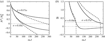
The evolution of the minimum of the buoyancy frequency obtained with the Gaussian beam approximation for internal and inertial waves is shown in figure 4(a). Two cases are shown for
 ${\it\sigma}=0.1{\it\omega}_{c}$
and
 ${\it\sigma}=0.17{\it\omega}_{c}$
(the same wave fields as those shown in figure 3
a). The inertial wave with broader frequency spectrum never reaches the convective instability, contrary to internal waves, which always reach the convective instability. Indeed, the initial amplitude of this broad frequency wave spectrum satisfies (3.8). The quasi-monochromatic inertial waves, for small
 ${\it\beta}$
, do reach the convective instability.
Evolution of (a) the minimum normalized buoyancy frequency and (b) the minimum Richardson number at each time. The Gaussian beam approximation for inertial waves is shown as a solid line and for internal waves as a dashed line. The wavepacket widths are
 ${\it\sigma}=0.1{\it\omega}_{c}$
and
 ${\it\sigma}=0.17{\it\omega}_{c}$
and the background flow is characterized by
 $\mathit{Ri}_{0}=100$
and
 $\tilde{f}=0.05$
.

3.3. Dynamical instability
Inertio-gravity waves may reach saturation through dynamical instability induced by the strong velocity shear of the wave field. The dynamical instability threshold may occur at a lower height than the convective instability (e.g. Dunkerton Reference Dunkerton1997) so that the breaking mechanism may differ from the characteristic wave overturning of internal gravity waves. In the last case, the convective instability occurs at regions of minimum shear (Hodges Reference Hodges1967). Howard (Reference Howard1961) and Miles (Reference Miles1961) showed that the necessary condition for the dynamical instability in an inviscid shear flow is that the Richardson number must be smaller than
 $\frac{1}{4}$
. In this work, we take the
 $\frac{1}{4}$
threshold for the instability assuming it is also a relevant reference value for gravity waves in a rotating frame. In the turbulence onset by an inertio-gravity wavepacket propagating upwards, Achatz (Reference Achatz2007) have identified non-modal perturbations with rapid growth even when the amplitude of the wave is not large enough to produce
 $\mathit{Ri}$
numbers smaller than
 $\frac{1}{4}$
. Thus, the threshold we use may be considered a (slightly) conservative value.
The Richardson number of the flow is defined as
 $$\begin{eqnarray}\mathit{Ri}=\frac{g{\it\theta}^{-1}\partial _{z}{\it\theta}}{(\partial _{z}u)^{2}+(\partial _{z}v)^{2}},\end{eqnarray}$$
where
 ${\it\theta}$
is the potential temperature of the flow, and
 $u$
and
 $v$
are the
 $x$
and
 $y$
components of the velocity of the flow.
We assume the flow is given by a background flow plus a perturbation,
 ${\it\theta}={\it\theta}_{0}+{\it\theta}_{1}$
and
 $(u,v)=(u_{0},0)+(u_{1},v_{1})$
. The perturbation is given by the solution of the Gaussian beam approximation for an inertio-gravity wave that propagates in a background flow. Then the Richardson number, (3.9), is
 $$\begin{eqnarray}\mathit{Ri}=\frac{\displaystyle \left[1+\left(\frac{k}{{\it\Omega}_{c}}a\right)\cos {\it\psi}_{c}\right]\left(1-\frac{f^{2}}{{\it\Omega}_{c}^{2}}\right)}{\displaystyle \left[\mathit{Ri}_{0}^{-1/2}\left(1-\frac{f^{2}}{{\it\Omega}_{c}^{2}}\right)^{1/2}+\left(\frac{k}{{\it\Omega}_{c}}a\right)\sin {\it\psi}_{c}\right]^{2}+\left[\frac{f}{{\it\Omega}_{c}}\left(\frac{k}{{\it\Omega}_{c}}a\right)\cos {\it\psi}_{c}\right]^{2}}.\end{eqnarray}$$
The phase
 ${\it\psi}_{c}$
that is taken in (3.10) is the one that gives the minimum Richardson number for each time. This determines the first time that the Richardson number threshold is reached in the wave field. In what follows, we always evaluate the Richardson number at the phase that gives the minimum value.
Figure 4(b) shows the evolution of the Richardson number for two wavepackets of different spectral widths, for the same cases as in figure 4(a). The inertio-gravity wave with
 ${\it\sigma}_{{\it\omega}}=0.1{\it\omega}_{c}$
reaches the dynamical instability at a similar time as the corresponding internal wave (the same wavepacket but in a medium without rotation) also attains the instability, which is expected to be a convective instability in this case (Hodges Reference Hodges1967). The inertio-gravity wave with
 ${\it\sigma}_{{\it\omega}}=0.17{\it\omega}_{c}$
only attains the dynamical instability. In the case of an internal gravity wave with this spectral width, it destabilizes the flow convectively at a later time than the inertial wave destabilizes the flow dynamically. These results show that Coriolis effects favour the development of the dynamical instability against the convective instability, particularly when the instability occurs at long times and close to the critical levels. This is in agreement with previous studies (Fritts & Rastogi Reference Fritts and Rastogi1985).
3.4. Height of the wave breaking
The height of the wave breaking is a critical parameter for gravity wave parametrizations (e.g. Alexander & Dunkerton Reference Alexander and Dunkerton1999). We thus examine the dependence of the breaking height on the wave and background flow parameters using the Gaussian beam approximation. The height of the threshold for convective instability
 $z_{s}$
is non-dimensionalized as
 $\tilde{z}_{s}=z_{s}/z_{cl}$
, where
 $z_{cl}$
is the height of the central critical level of an internal gravity wave (so that the results can be compared directly between inertial and internal waves).
Using the convective instability condition, (3.6), with the wave amplitude given by (3.1), and then expressing it as a function of
 $z$
by means of (2.20), the threshold for convective instability
 $\tilde{z}_{s}$
is constrained by
 $$\begin{eqnarray}{\it\beta}^{4}=\frac{{\tilde{u}}^{4}(1-\tilde{f}^{2})^{3}-[(1-\tilde{z}_{s})^{2}-\tilde{f}^{2}]^{3}}{\left\{\left[\displaystyle \frac{(1-\tilde{z}_{s})^{2}-\tilde{f}^{2}}{1-\tilde{f}^{2}}\right]^{3/2}-(1-\tilde{z}_{s})\right\}^{2}}.\end{eqnarray}$$
Equation (3.11) gives the convective threshold height as a function of the transient wave parameters
 ${\it\beta}$
,
 $\tilde{f}$
and
 ${\tilde{u}}$
. For
 $\tilde{f}\rightarrow 0$
, the convective threshold height given for internal waves in Pulido & Rodas (Reference Pulido and Rodas2008) is recovered from (3.11).
The height at which the transient wavepacket reaches the threshold of dynamical instability,
 $\tilde{z}_{d}=z_{d}/z_{cl}$
, is defined as the height obtained from (2.20) evaluated at the (minimum) time at which
 $\mathit{Ri}$
, from (3.10), reaches the value 0.25. This threshold is taken as a mean reference value, but note that Achatz & Schmitz (Reference Achatz and Schmitz2006) and Fritts et al. (Reference Fritts, Vadas, Wan and Werne2006) show that turbulence can be produced by gravity waves at larger Richardson number values. It is not possible to obtain an expression for
 $\tilde{z}_{d}$
analytically, so that a numerical algorithm is employed to obtain
 $\tilde{z}_{d}$
as a function of the wave parameters.
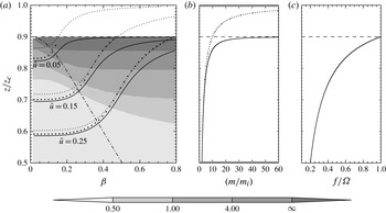
Figure 5(a) shows the height where the dynamical (continuous line) and convective (large dots) instabilities for inertial waves are attained as a function of
 ${\it\beta}$
(a measure of the transient effects in the wave). The height of the convective instability threshold for internal waves is also shown (dotted line, small dots). For inertial waves, the case with
 $\tilde{f}=0.1$
is taken. The height of the lowest inertial critical level of the central component of the wavepacket for this case is
 $0.9z_{cl}$
. The shaded contours represent the time difference between the time that the wave requires to reach the dynamical instability threshold and the time for the convective threshold. The time required to develop the dynamical instability depends on the growth rate. Therefore, the time required for the wave to reach the dynamical instability threshold plus the time required for the instability development must be shorter than the time required to reach the convective threshold if the dynamical instability mechanism is dominant. A long time difference between the dynamical instability threshold and the convective threshold shows that the dynamical instability mechanism is more likely to be dominant for the same growth rate.
(a) Height of the dynamical instability threshold
 $\tilde{z}_{d}$
(solid) and of the convective threshold
 $\tilde{z}_{s}$
(larger dots) as a function of
 ${\it\beta}$
for different initial amplitudes
 ${\tilde{u}}=0.05,\ 0.15,\ 0.25$
. The height of the convective instability threshold for internal waves is shown with a dotted line. The height at which the maximum amplitude of the wavepacket is achieved is shown with a dashed-dotted line. The shaded contours represent the time difference between the dynamical instability threshold and the convective threshold. (b) Vertical wavenumber as a function of height for inertial waves (solid) and for internal waves (dotted). (c) Plot of
 $f/{\it\Omega}$
as a function of height.

Figure 5 gives a general picture of the importance of inertial effects for wave breaking. Waves that reach the instability threshold far from the critical level are not affected by the inertial effects. Specifically, far from the inertial critical level, the inertial waves for small
 ${\it\beta}$
attain the convective instability practically at the same height as the internal waves. We identify the transition roughly at
 $\tilde{z}_{s}<0.7$
. An extensive analysis of the wave breaking mechanisms for internal waves in the same context is given by Pulido & Rodas (Reference Pulido and Rodas2008). The present results show that the analysis for internal waves is also valid for inertial waves with small
 ${\it\beta}$
that break far from the critical level. In particular, given the agreement found between the internal and inertial waves, these waves for
 $\tilde{z}_{s}<0.7$
are expected to break through convective overturning for small
 ${\it\beta}$
. Note that
 $\mathit{Ri}$
also becomes zero when
 $N^{2}$
attains the convective overturning, but in this case the height of the threshold is close to the wave phase of minimum shear for internal waves (Hodges Reference Hodges1967).
Figure 5(b) shows that the central vertical wavenumber is relatively the same for internal and inertial waves at the height of the breaking for
 $\tilde{z}_{s}<0.7$
. Both the central vertical wavenumber and the central intrinsic frequency only depend on height, so that waves that attain the threshold at a given height for any combination of the parameters
 ${\it\beta}$
and
 ${\tilde{u}}$
break with the same central vertical wavenumber and central intrinsic frequency. From figure 5(c), the central intrinsic frequency at the breaking height,
 ${\it\Omega}_{b}$
, for
 $\tilde{z}_{s}<0.7$
is
 $f/{\it\Omega}_{b}<0.35$
, in agreement with the results found by Dunkerton (Reference Dunkerton1997). For any practical application, e.g. gravity wave parametrizations, waves in the atmosphere that break with
 $f/{\it\Omega}_{b}<0.35$
and small
 ${\it\beta}$
are well represented by the non-rotating assumption.
On the other hand, the breaking threshold for inertial waves that reach the instability close to the critical level
 $z/z_{cl}>0.7$
, which corresponds to
 $f/{\it\Omega}_{b}>0.35$
(see figure 5
c), occurs at lower heights than for internal waves. For these cases, the dynamical instability threshold for inertial waves is attained at lower heights than the convective instability condition. Therefore, there are two effects that act jointly to give a lower breaking height for highly transient inertial waves with respect to internal waves: the appearance of the inertio-critical level at a height lower than the classical (non-inertial) critical level; and that the dynamical instability condition is met at a lower height than the convective instability condition. The height and time differences between the dynamical and convective breaking thresholds increase for larger
 ${\it\beta}$
.
Waves with large
 ${\it\beta}$
that reach the instability threshold for
 $z/z_{cl}>0.86$
in figure 5(a) satisfy the condition (3.8), so that they do not attain the convective instability and they break through dynamical instability. This is shown in figure 5(a) with the dark shading contour. Transient effects are important for inertial waves that reach the instability criterion at a higher altitude than the maximum amplitude height (dashed-dotted line in figure 5
a). In this case the amplitude of the wavepacket is expected to be small and the time difference between the time required to meet the dynamical instability and the convective instability time increases for larger
 ${\it\beta}$
. For instance, for
 $\tilde{z}_{s}=0.8$
the time difference is less than 1 h for small
 ${\it\beta}$
while it is 4 h for large
 ${\it\beta}$
, indicating that these highly transient waves are likely to break through dynamical instability instead of convective instability. Therefore, while the (upper) threshold for the dynamical instability is
 $\tilde{z}_{s}>0.86$
for medium-range
 ${\it\beta}$
, the (upper) threshold is expected to be somewhat smaller, say
 $\tilde{z}_{s}>0.75$
, for highly transient waves, large
 ${\it\beta}$
, considering the height and time differences between the dynamical and convective instabilities.
For waves that propagate close to the inertio-critical level, dissipation by viscosity and thermal conductivity becomes a dominant factor. A readily performed calculation, assuming a constant kinematic viscosity of
 ${\it\nu}=10^{-3}\ \text{m}^{2}\ \text{s}^{-1}$
, which is a representative value in the atmosphere at 33 km height, gives that the waves have lost 10 % of their amplitude at a height of
 $z/z_{cl}=0.88$
. For altitudes higher than
 $z/z_{cl}=0.88$
, the dissipative effects should be considered.
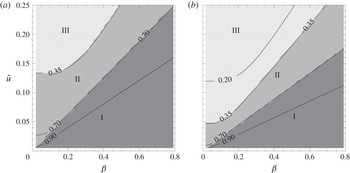
Figure 6(a) shows the breaking regions as a function of
 ${\it\beta}$
and
 ${\tilde{u}}$
for
 $\tilde{f}=0.1$
for which the convective or dynamical instability criteria are satisfied. Three regions are identified in the figure.
-
(i) For waves with a small
 ${\tilde{u}}/{\it\beta}$
ratio, as specified in (3.8) and shown in figure 6(a) with dark grey shading, the convective instability is never met. Thus, an inertio-gravity wavepacket that propagates towards its critical level in this region is expected to produce a dynamical instability with characteristics similar to the instabilities found by Lelong & Dunkerton (Reference Lelong and Dunkerton1998a
). The limit of this region is a straight line with a slope of
$\tilde{f}^{1/2}/(1-\tilde{f}^{\,2})^{3/4}$
, which coincides with
$f/{\it\Omega}_{b}=0.7$
except for small
${\it\beta}$
. This limit for
$\tilde{f}=0.1$
corresponds to
$\tilde{z}_{s}=0.86$
, except for small
${\it\beta}$
.
-
(ii) There is an intermediate region, which is composed of inertio-gravity wavepackets with intrinsic frequency in the range
$0.35<f/{\it\Omega}_{b}<0.70$
. The instability to be initiated by the wave in this region is a hybrid between convective and dynamical instabilities (Dunkerton Reference Dunkerton1997). The dominant behaviour will depend on the growth rate of the dynamical instability, so that the time needed by the dynamical instability to be developed occurs before the convective instability criterion is reached. -
(iii) In the large-amplitude extreme, for transient inertial waves with
${\tilde{u}}$
and
${\it\beta}$
located in the region above the
$f/{\it\Omega}_{b}=0.35$
curve (the light shaded region in figure 6
a), these waves have similar propagation characteristics to internal waves, so that we expect the breaking of these waves to be dominated by convective instability.





Instability regions for transient inertio-gravity waves as a function of
 ${\tilde{u}}$
and
 ${\it\beta}$
for (a)
 $\tilde{f}=0.1$
and (b)
 $\tilde{f}=0.05$
. Wavepackets that reach instability for
 $f/{\it\Omega}_{b}=0.2$
, 0.35, 0.7 and 0.9 are represented with solid lines. The shaded dark grey region (region I) represents wavepackets that only reach dynamical instability. The light grey region (region III) represents wavepackets for which the inertial effects, even close to the convective instability threshold, may be considered negligible. The intermediate region (region II) represents wavepackets that do not have a dominant criterion, so that a hybrid convective–dynamical instability may be expected in this regime.

If
 $\tilde{f}$
is diminished (wavepackets with higher central frequency), as shown in figure 6(b), the slope of regime I limit is diminished, see (3.8), but the breaking frequency does not change,
 $f/{\it\Omega}_{b}=0.70$
. The hybrid regime, region II, is narrower. The convective instability is dominant (region III) in this small
 $\tilde{f}$
case for smaller wave amplitudes
 ${\tilde{u}}$
. Figure 6(a,b) also shows that the dynamical instability is more likely to be developed for transient waves with broader spectral width. In other words, wavepackets with larger
 ${\it\beta}$
and the same initial amplitude
 ${\tilde{u}}$
attain the dynamical instability with larger
 $f/{\it\Omega}_{b}$
so that the inertial effects are more important.
3.5. Propagation in a realistic environment
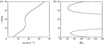
The performance of the Gaussian beam approximation is evaluated in a realistic environment. We examine the propagation of a Gaussian wavepacket in a background wind that is a realistic smoothed zonal wind profile characteristic of high latitudes in winter in which the subpolar and the stratospheric nocturnal jet are both present. The zonal background wind profile is shown in figure 7(a). This is a particularly difficult case since the zonal wind is non-monotonic. The background buoyancy frequency and Coriolis parameters are typical values,
 $N_{0}=0.02\ \text{s}^{-1}$
and
 $f=10^{-4}\ \text{s}^{-1}$
. The background Richardson number as a function of height is shown in figure 7(b). A wavepacket with initial parameters
 ${\it\sigma}_{{\it\omega}}=0.1{\it\omega}$
,
 ${\it\omega}=N_{0}/10$
and
 ${\it\omega}/k=55\ \text{m}\ \text{s}^{-1}$
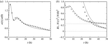
is launched in this environment. The evolution of the normalized amplitude is shown in figure 8(a). The amplitude of the wavepacket achieves two local maxima. Both peaks in amplitude are achieved when the wavepacket is in the height ranges where the background zonal wind increases with height. These two maxima are produced due to refraction and dispersion effects. In altitudes where the background zonal wind increases with height, refraction effects produce an increase of the amplitude. At the same time, the highest components of the wavepacket are in a stronger background wind so that their group velocity diminishes with respect to the components that are in the lower part of the envelope. Therefore, the dispersion effects are weaker in regions where the background zonal wind increases. The amplitude given by the Gaussian beam approximation shows a close agreement to the numerical integration (figure 8
a). Indeed, the oscillation that appears in the numerical integration at long times is an artifact, so the Gaussian beam approximation probably gives a better field than the numerical experiment (see Pulido & Rodas (Reference Pulido and Rodas2008) for a discussion of this numerical error). The evolutions of the Richardson number and buoyancy frequency are shown in figure 8(b). The case has only dynamical instability, while convective instability is never reached. A close agreement between the Gaussian beam approximation and the numerical solution is found particularly for the buoyancy frequency evolution.
(a) Background zonal wind as a function of height and (b) background Richardson number.

(a) Amplitude evolution of an inertial wavepacket with
 ${\it\sigma}=0.1{\it\omega}$
that propagates in the background zonal wind shown in figure 7 for the Gaussian beam solution (solid line) and the numerical experiment (triangles). (b) Minimum Richardson number (same curve convention as amplitude) and the minimum normalized buoyancy frequency for the Gaussian beam solution (dashed line) and the numerical experiments (diamonds).

4. Conclusions
The instabilities developed by inertio-gravity waves that propagate in a shear flow towards the critical level as a function of wave and background parameters have been studied in previous works under the steady-state assumption. In this work, the propagation of transient inertio-gravity waves that propagate in a shear flow towards the critical level is examined using the Gaussian beam approximation. This approximation permits one to obtain a general picture of the propagation and the triggering of breaking mechanisms of transient inertio-gravity waves as a function of the wave and background parameters. We prove that inertial effects are enhanced for transient waves compared to steady-state waves. We have first considered a flow configuration that is simple but important: a constant vertical shear. For this case, results with the Gaussian beam approximation may be obtained analytically. The Gaussian beam approximation is also useful for realistic wind profiles, for which a simple numerical vertical integration is needed that evaluates (2.19). The approximation in this realistic case gives very close agreement compared with an expensive high-resolution numerical model (which gives a noisier solution).
Inertio-gravity wavepackets that propagate towards the critical level and attain the instability threshold with the same
 ${\it\Omega}_{b}$
(the central intrinsic frequency at the breaking height) may have different dominant instabilities depending on the spectral width of the packet. In particular, the time separation between the convective and dynamical instabilities depends on the frequency width. Wavepackets with small initial amplitude reach their instability threshold close to the inertio-critical level, so that they require a very long time to arrive and viscous diffusion may be dominant in the dissipation of those small-amplitude and highly transient wavepackets as found in numerical simulations by Winters & D’Asaro (Reference Winters and D’Asaro1994).
Mountain waves that propagate in a horizontal background flow that is rotating with height also find critical levels at different heights for different components of the horizontal wavenumber spectrum. In this case, the wave energy density decays asymptotically to zero when the mountain waves propagate in a rotating background flow towards the critical levels (Shutts Reference Shutts1998; Broad Reference Broad1999). Therefore, some similarity is expected in the breaking mechanism of mountain waves that propagate in a flow that rotates with height with the breaking of transient gravity waves in a shear flow. The Gaussian beam approximation has been applied to orographic waves by Tanushev et al. (Reference Tanushev, Quian and Ralston2007) and Pulido & Rodas (Reference Pulido and Rodas2011).
At long times, the Gaussian beam approximation gives the same asymptotic tendency as the standard spatial ray tracing theory. The most important benefit of the Gaussian beam approximation in this work is that it can detect the maximum amplitude achieved at short times by the inertial wavepacket that propagates towards the critical level. This approximation permits a whole treatment of the propagation of the waves from the initial time up to the achievement of an instability threshold (beyond this time the linear theory is not valid). This is an important difference with the standard spatial ray tracing approximation, which can only represent the asymptotic behaviour of the wave field and therefore the wave maximum amplitude is not detected. To capture this maximum amplitude of the disturbance is essential for determining the time and height of the convective and dynamical instabilities of transient inertio-gravity waves. Alternative methods based on ray tracing theory like the formulation by Hayes (Reference Hayes1970) of the derived ray equation and the integral representation proposed by Broutman et al. (Reference Broutman, Rottman and Eckermann2001) for the near field (short time in our context) could also be used to represent the maximum amplitude at short times.
The Gaussian beam formulation is applied in this work to a transient inertio-gravity wavepacket that is localized in time and characterized by a frequency width. The treatment of a general disturbance in this formulation can be derived from the temporally localized wavepacket examined in this work. General disturbances, which have extended frequency spectra, can be represented through a superposition of Gaussians in the spectral space. The width of the Gaussians corresponds to the width of the bins into which the frequency spectrum of the disturbance is divided. The solution of the disturbance in the physical space is given in this case by the superposition of the Gaussian beam solutions. This procedure of Gaussian superposition in the spectral space is explained in detail and applied to orographic waves generated by a realistic orography in Pulido & Rodas (Reference Pulido and Rodas2011).
The Gaussian beam approximation is a powerful tool that can be implemented as a ray tracing gravity wave model. Current ray tracing gravity wave models applied to the atmosphere, such as GROGRAT (e.g. Marks & Eckermann Reference Marks and Eckermann1995; Eckermann & Marks Reference Eckermann and Marks1997) and that of Hasha, Bühler & Scinocca (Reference Hasha, Bühler and Scinocca2008), make a strong assumption that the cross-sectional area of ray tubes is constant along the ray path. This approximation is taken to avoid the singularities that appear when rays intersect, i.e. at caustics. Under the assumption of a constant cross-sectional area, the effects of dispersion on the wave amplitude field, in particular by horizontally varying background winds, are not considered. The problems of ray tracing in caustics have been extensively treated in the gravity wave literature (e.g. Broutman Reference Broutman1984, Reference Broutman1986; Sonmor & Klaasen Reference Sonmor and Klaasen2000). One of the techniques proposed to avoid caustics is the Maslov method, in which the wave field is mapped to the Fourier space at caustics. It has been applied successfully for mountain waves (Broutman, Rottman & Eckermann Reference Broutman, Rottman and Eckermann2002). The Gaussian beam approximation is free of caustics and therefore it is also suitable for detecting and evaluating realistic ray focusing in the atmosphere and the ocean.
The implementation of the Gaussian beam approximation described in this work cannot consider the effects of a horizontally non-uniform background flow, except for the refraction produced by a horizontally non-uniform background flow in the path of the ray. The focusing and diffraction effects produced by the differential dispersion of horizontally non-uniform background flows that impact in the determination of the amplitude of the wave field (say in the last term on the right-hand side of (2.22)) are not captured in the current implementation of the Gaussian beam approximation. An Eulerian representation of the Gaussian beams instead of ray centred coordinates may be essential to represent these effects.
In this work, we have achieved a generalization to the full frequency range of gravity waves with respect to a previous work (Pulido & Rodas Reference Pulido and Rodas2008), a necessary step towards our main aim, which is the development of a gravity wave parametrization for atmospheric models based on the Gaussian beam approximation. This approximation applied to inertio-gravity waves may account for the long horizontal propagation found for inertio-gravity waves observed in high latitudes and in particular in South America (Dunkerton Reference Dunkerton1984; Sato et al. Reference Sato, Tateno, Watanabe and Kawatani2012; Pulido et al. Reference Pulido, Rodas, Dechat and Lucini2013). An important further step in the development of such a gravity wave parametrization based on the Gaussian beam formulation is the consideration of time-dependent and horizontally varying background winds, effects that can give more realistic momentum depositions (Dunkerton & Butchart Reference Dunkerton and Butchart1984; Senf & Achatz Reference Senf and Achatz2011).
The application of the Gaussian beam approximation goes beyond the oceanic or atmospheric gravity waves conducted in this work. It is a powerful tool that can be applied to other fields. Indeed, it has been applied for a long time in geophysical problems (see a review by Kravtsov & Berczynski (Reference Kravtsov and Berczynski2007)) and it has been proven to be useful in optics and quantum mechanics.