

1 Introduction
A fundamental problem of intergenerational relationships within families arises from the inability to write binding contracts with minors. As a consequence, parents cannot capture the returns to their human capital investment efforts that accrue to their children. While informal transfer rules within the family may be established, parents generally cannot enforce that their children meet their transfer obligations. Obviously, this situation will typically lead to underinvestment in the children's human capital. One policy to combat this problem is to provide public schooling where the costs are socialized by letting all adults pay taxes to finance the schools. In addition, a public intergenerational transfer scheme is created in which the parent generation benefits from these investments, which typically takes the form of a pay-as-you-go (PAYG) pension scheme. In such a system, the contributions paid by workers are immediately spent on current pensioners. Thus, the PAYG pension scheme can be rationalized as an enforcement device to ensure sufficiently high transfers from children to their parents (Sinn, Reference Sinn2004). However, the creation of a PAYG scheme in combination with a public school system does not solve the underlying incentive problem completely. The usual pension formulas that provide a lump-sum benefit or tie benefits to previous own contributions do not address human capital acquisition within families that cannot be observed by the government. Moreover, the PAYG scheme gives rise to fiscal externalities.
Investing in the quantity and quality of children is associated with positive fiscal externalities when a PAYG pension scheme is in place. With given social security contribution rates, total contributions rise both with a higher number of and with higher productivity of contributors. Hence, when individuals decide to have children or to provide them with human capital, utility levels of other individuals in the same generation will rise through higher expected pension claims. Consequently, people tend to invest too little in the number and quality of their children.
Our paper addresses the question of how the pension formula has to be adapted in order to incorporate the externalities in some sense of optimality. The notion of optimality is vague here because the Pareto criterion cannot be applied in a framework of endogenous fertility, and a generally accepted alternative does not exist (Golosov et al., Reference Golosov, Jones and Tertilt2007). As some individuals do not exist in all allocations, a meaningful comparison of their utility levels is impossible. Following a typical way out of this dilemma, we maximize a utilitarian welfare function. While other policy instruments such as family allowances or scholarships for talented students may serve the same purpose as specific pension benefits, it is interesting to find out the consequences if the internalization takes place only in the pension scheme. The analysis allows conclusions with respect to the use of alternative policy instruments, as equivalent instrument sets can be constructed. In our study, the goal is to maximize the sum of expected utilities in the parent generation given a fixed social security contribution rate on wages. We do not discuss the choice of the optimum size of the PAYG scheme. As the currently old are not affected by a change in the pension formula that becomes effective in the next period, their interests can be ignored. We consider an economy with heterogeneity in productivity where the outcomes of investment in both fertility and education are stochastic.
In addition to the externality problem, it has been noted that the extension of public pensions drives down fertility. Public pensions crowd out transfer schemes within families. If individuals do not care about the wellbeing of their offspring, the smaller transfers old parents receive from their children reduce the demand for children (Cigno, Reference Cigno1993). The same prediction turns out if parents are altruistic toward their children provided that the economy is in a dynamically efficient situation, that is when the rate of return in a PAYG scheme falls short of the interest rate. While parents would like to compensate their children for the social security transfer, the implicit tax on contributions raises the price of a child, reducing the demand for children (Becker and Barro, Reference Becker and Barro1988). Empirical evidence for the negative impact of social security on fertility is presented in Cigno and Rosati (Reference Cigno and Rosati1996), Cigno et al. (Reference Cigno, Luporini and Pettini2003), and Boldrin et al. (Reference Boldrin, De Nardi and Jones2005).
When applying the fiscal externality argument to schooling, it is often not seen as relevant at the margin. The asymmetry of fertility and education is a consequence of differences in policy interventions. Many countries have already adopted some type of child benefit in the pension formula, but the size of these benefits is much smaller everywhere than the contributions of the child to the pension system. At the same time, schooling is subsidized at a rate of almost 100%. In our analysis, we ignore observable education and focus on human capital acquisition within the family. As lots of studies stress the importance of the family background when explaining educational outcomes (for example, Woessmann, Reference Woessmann2008), setting incentives for unobservable education effort at home seems to be quite appropriate.
In order to keep the analysis simple, we investigate a framework of a small open economy with a stationary technology. We ignore impacts of changing parameters of the PAYG pension system on growth via savings, which have been discussed in endogenous growth settings by Zhang (Reference Zhang1995) and Wigger (Reference Wigger1999). With this simplification, we rule out externalities of fertility decisions and education efforts working via changing factor prices. Both fertility and the individual's productivity are stochastic, where in each case the level of investment affects the probability distribution of outcomes. As a result, we have both high and low productive households, with and without children. The direct cost of providing a child with a given level of education is lower for high productivity parents. With this assumption, our model can reproduce the stylized fact of a positive intergenerational correlation of productivities across families (Gradstein et al., Reference Gradstein, Justman and Meier2005: ch. 3). The heterogeneity of individuals enables us to study the impacts of financial incentives on different groups. It is not obvious how an ‘optimum’ mix of encouraging fertility and education should look like. Individuals first choose the level of their fertility investment. After the number of children is known, people decide on savings and human capital investment. The preference structure is in line with the quantity–quality model of demand for children (Becker and Lewis, Reference Becker and Lewis1973). Some intrinsic motivation for having children and a preference for letting them arrive at a high productivity will yield positive investment in the quantity and quality of human capital even in the absence of financial incentives. The pension consists of up to four components: a share contingent on previous earnings, a benefit that depends on the number of children, a component that assigns parts of the children's contributions to their parents, and a flat benefit. Individuals exhibit quasi-linear preferences. The obvious drawback of this specification is the exclusive impact of income changes on working age consumption. This problem may be outweighed by the advantage that utilities can simply be added in the welfare analysis, where results are not driven by distributional aspects within a generation.
With this specification, increasing fertility-related pensions will lead to a larger number of children, while not affecting the educational effort levels of parents. In contrast, a higher share of children's contributions directly transferred to their parents will yield both more human capital investment and a higher number of children. The latter result is a consequence of the fact that children become more profitable for their parents.
In any first-best allocation, investment in fertility and education will be increased to the level where the marginal cost is equal to the aggregate marginal benefit arising for the parent generation. At the same time, old age consumption is perfectly smoothed across all states. The former optimality condition requires incentives for investment in education. However, using such incentives implies that consumption smoothing will not be achieved when the outcome of the investment decision is uncertain. The second-best scheme therefore displays the property that parents collect some of their children's contributions, but not the full amounts. As some underinvestment in fertility would otherwise occur, the optimum scheme is also associated with some fertility-related component. With this component, the PAYG scheme insures against the risk of an unfortunate outcome of educational efforts. As a consequence of risk pooling, the public pension scheme is superior to just mimicking the transfer rules of a family constitution.
The standard message of the literature on PAYG pensions and endogenous fertility is that an internalization of the positive externality requires that the full PAYG pension is made contingent on fertility (Kolmar, Reference Kolmar1997). This result carries over to several alternative specifications, such as allowing for migration (Kolmar, Reference Kolmar2001) or decision-making by couples (Abio et al., Reference Abio, Mahieu and Patxot2004). As an alternative, family allowances can be introduced being equal to the present value of a child's contribution (van Groezen et al., Reference van Groezen, Leers and Meijdam2003; van Groezen and Meijdam, Reference van Groezen and Meijdam2008). This amount represents the net social gain of an additional individual given that her pension will be financed by her children (Sinn, Reference Sinn2001).
In some recent papers, several arguments have been given, under which circumstances the standard proposition will fail. First, a stronger fertility incentive can reduce lifetime labor supply, imposing a negative externality on the older generation through declining pensions (Fenge and Meier, Reference Fenge and Meier2005 and Reference Fenge and Meier2008). Second, if the outcome of the fertility decision is stochastic, the optimum scheme sets milder fertility incentives in order to decrease the income risk (Cremer et al., Reference Cremer, Gahvari and Pestieau2006a). Third, if individuals exhibit cost differences in raising children, a utilitarian government will choose to redistribute towards high cost individuals, which again calls for less fertility-related pensions (Cremer et al., Reference Cremer, Gahvari and Pestieau2006b).
Few attempts have been undertaken to study the interactions of fertility, investment in human capital, and PAYG pensions. Peters (Reference Peters1995) analyzes a closed economy framework in which the government can subsidize private education. He finds a quantity–quality tradeoff, and argues that education will always be subsidized, while fertility may be taxed. The contributions closest in spirit to our analysis are Cigno et al. (Reference Cigno, Luporini and Pettini2003), Barbie et al. (Reference Barbie, Hagedorn and Kaul2006), and Cigno and Luporini (Reference Cigno and Luporini2006). The former discusses a framework in which parents can deterministically choose the number of children and an action that affects the child's tax-paying capacity in a stochastic fashion. While the government can force the individuals to choose the optimum number of children, transfers to parents are made contingent on the child's performance, for example by a scholarship. Barbie et al. (Reference Barbie, Hagedorn and Kaul2006) analyze a framework with exogenous fertility, where investment in education is associated with a stochastic outcome. They stress the role of social security to insure against the productivity risk, where only part of the pensions are contingent on the children's wages. Our contribution generalizes their analysis by investigating the case of stochastic and endogenous fertility. As in our paper, Cigno and Luporini (Reference Cigno and Luporini2006) introduce stochastic fertility and cost differences across parents in providing their children with human capital. The optimum tax-transfer scheme is associated with payments contingent on the child's performance and a purely fertility-related component to insure parents against an unfortunate outcome of their human capital investment decision. These features appear again in our framework in which we apply quite a similar structure to the specific problem arising in the PAYG pension scheme. We depart from the analysis of Cigno and Luporini in two respects. First, we add heterogeneity in income in the parent generation that determines the private cost of educating children, which is therefore observable for the government. Our specification constitutes a plausible alternative, which has no major impact on the results, however. Second, we eliminate the government's motive for income redistribution by imposing quasi-linear preferences. Therefore, the results reflect only allocative issues. In our framework, it unambiguously turns out that households with a lower cost of educating children will receive a higher expected pension. This does not necessarily hold in Cigno and Luporini (Reference Cigno and Luporini2006) because the government's motive to redistribute from the rich to the poor calls for higher transfers to poorer households. Both approaches share the property of second-best allocations that households with a lower cost of educating children will invest more in fertility.
The remainder of the paper is organized as follows. Section 2 introduces the model. The comparative static analysis in Section 3 discusses the impacts on changing parameters in the pension formula on saving, fertility, and human capital investment. Section 4 deals with the structure of first-best allocations and shows that welfare losses will necessarily arise in our imperfect information framework. In the following Section 5, second-best pension schemes are characterized. The final Section 6 discusses the main findings.
2 The model
We consider a small open economy where the rate of interest and the wage rate for one efficiency unit of labor are determined at the world market. In order to analyze fertility choices, we employ a three-period overlapping generations model. For simplicity, we consider a one-sex population consisting of females. A generation lives for three periods. In the first period, an individual lives with her parent. She receives an education level e, which is chosen by her mother.
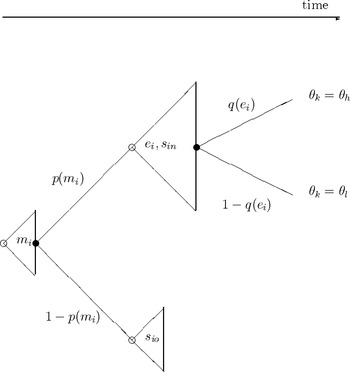
In the second period, the productivity of the individual is revealed, being either high, θh, or low, θl, with θl<θh. An individual of type i∊{h, l} supplies one unit of labor and receives a gross wage income θi. The wage rate for one efficiency unit of labor is normalized to one. Furthermore, the household of type i chooses the investment m i that affects the expected number of children she will have in this period.Footnote 1 In contrast to Cigno and Luporini (Reference Cigno and Luporini2006), the activity translates into an expenditure, which serves to avoid corner solutions in the absence of a PAYG scheme. The fertility investment reflects all costs associated with pregnancies that have to be borne by the individual, for example due to medical investigations, special treatments, or miscarriages. The outcome of the fertility investment, represented by the number of children, is stochastic. With probability p i=p(m i), the realized number of children will be n, with n>0. In the opposite event, occurring with probability 1−p i the number of children will be zero. The fertility investment increases the probability of having children, i.e. p i′>0, but at a decreasing rate, p i″<0. Raising one child is associated with a cost K.
Knowing the realized number of children j with j∊(0, n) a household of type i decides how much to save, s ij, and to consume, c ij, and, provided that there are children, how much to invest in the education of each child, ρ(θi)e i. The cost of providing children with a given level of education varies according to the productivity of the mother, with ρ′<0. The cost advantage of high productivity parents reflects either possible genetic factors or the home environment, as factors in human capital production explaining the observable intergenerational correlation of abilities. Our assumption expresses that high productivity parents are better at teaching their children during their leisure time. Of course, the higher opportunity cost for these parents would call for ρ′⩾0. A positive correlation between the productivity of the mother and the cost of educating children would alter the comparative static results on differences between low productivity and high productivity parents and would also change the structure of first-best allocations with respect to education effort and fertility investment. However, a positive sign of ρ′ would not affect our main result in Proposition 1 on properties of a linear second-best pension scheme.
The outcome of the investment depends on the input in a stochastic fashion. With probability q i=q(e i), all siblings will have high productivity θh. Otherwise, with probability 1−q i, all siblings end up with productivity θl. The assumption of perfect correlation across siblings is just taken for simplicity. Assuming uncorrelated draws or imperfect positive correlation of productivities instead would certainly be more realistic. Such alterations would not affect the nature of second-best pension schemes in a qualitative sense, however. To ensure a unique positive investment level, the human capital production function exhibits the properties q i′>0, q i″<0, lime→0q i′=∞. Finally, an adult has to pay contributions to the PAYG pension system in her working period, where the contribution rate is τ. Hence, consumption in the second period is given by

without and with children, respectively. We assume that the minimum net income (1−τ)θl exceeds the cost of raising children, nK, by a substantial amount to ensure that the latter can be financed without borrowing against future pension claims.
In the third period, a mother of type i with n children of type k retires and consumes z ink. Old age consumption equals the sum of private savings multiplied by the interest factor R and the pension πink:

A childless retiree receives a pension πi0 and consumes z i0=Rs i0+πi0.
Since our focus is not on intra-generational redistribution, but on the relationship between, on the one hand, the PAYG system and, on the other hand, fertility and education, we assume quasi-linear preferences. As a consequence, the aim to redistribute between rich and poor does not complicate the results. A childless woman and a mother of type i with n children of type k achieve utility
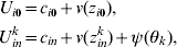
respectively, where v′>0, and v″<0. As we are mainly interested in consumption uncertainty induced by the pension formula, quasi-linear utility is specified as linear in working age consumption rather that in old age consumption. The function ψ measures how the existence of children and the productivity of children directly increase the utility of their mother, where 0<ψ (θl)<ψ (θh). As indirect utility of an individual is fully determined by her type, the function ψ can also be interpreted as expressing altruism towards the individual's children. In the absence of this consumption motive, nobody would invest in fertility or education unless the design of the pension formula creates an investment motive. Provided that the cost of raising a child falls short of the present value of her future minimum contribution, K<τθl/R, the features of the second-best pension schemes described in the proposition continue to hold in an environment without altruism. Denoting expected utility after the number of children is revealed by

expected lifetime utility is simply

where utility in the first period, when no decision is taken, is omitted.
The state-run PAYG pension system relates pensions to previous own contributions, number of children, contributions of children, and a flat component according to the formulas
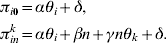
The pension parameters are restricted by α⩾0, β⩾0, 0⩽γ⩽τ. If γ were larger than τ, total benefits based on own children's contributions would exceed total contributions to a PAYG scheme.
Each adult solves a two-stage decision problem. First, she maximizes lifetime utility through a decision on fertility investment. Second, after revelation of the number of children, she chooses education effort and savings so as to maximize contingent expected utility, as given by (4). A solution is determined by backward induction. Figure 1 summarizes the sequence of decisions.
Sequence of Decisions

Due to the properties of the probability functions and the utility function, it is natural to assume interior solutions. Hence, working age consumption, old age consumption, fertility investment, and educational effort will all be positive.Footnote 2 According to whether or not the fertility investment has led to births, the contingent first-order conditions for savings are


The equations state that the marginal expected rate of substitution between old age consumption and working age consumption will be equal to the relative price 1/R. Obviously, the same consumption level in old age turns out irrespective of previous productivity for childless individuals, z l0=z h0. Furthermore, old age consumption of individuals of a given productivity type varies both with the number and type of children if and only if γ>0.
Choosing the educational investment per child is of course only relevant for individuals with children. The type-specific first-order conditions are given by

In the optimum, the marginal cost associated with one additional unit of education effort in the second period, nρ(θi), is equal to the expected marginal benefit. The latter arises through an increased probability of high productivity children according to q′(e i). Parents prefer to have high productivity children for its own sake, as expressed by ψ(θh)−ψ(θl)>0. Moreover, their old age consumption may increase if their children's contributions have a direct impact on their pension, where the utility gain is given by v(z inh)−v(z inl).
Finally, the first-order condition for optimal fertility investment is

Investing one additional dollar in fertility directly reduces working age consumption. It increases the probability of n births according to p′(m i). Having these n children will be associated with direct costs nK, and costs of education nρ(θi)e i. Saving then changes from s i0 to s in. If the education effort turns out to be successful, which happens with probability q(e i), the household will arrive at utility from old age consumption and children as given by v(z inh)+ψ(θh). The respective values for parents with less productive children and childless individuals are v(z inl)+ψ(θl) and v(z i0).
3 Comparative statics
In this section, we briefly analyze the effects of parameter changes on individual behaviour, where no measures are taken to balance the budget of the pension system. Comparative static results on the impacts of changes in the flat pension, the contribution-related pension, and the fertility-related pension are summarized in Lemma 1.
Lemma 1
Increasing either the lump-sum pension, δ, or the contribution-related pension, αθi, leads to a compensating fall in savings, where all old age consumption levels, z i0, z inh, z inl, educational investment, e i, and fertility investment, m i, are unchanged. Increasing the fertility-related pension, βn, does not affect savings of childless individuals, s i0, induces a compensating fall in savings of individuals with children, s in, leaves educational investment per child unchanged, and increases the fertility investment level.
Proof
See Appendix A. □
Due to the specification of the quasi-linear utility function and the assumption that income suffices for having positive working age consumption, all income increases are exclusively used to raise working age consumption. A rising fertility-related pension increases the marginal benefit of a child. Hence, increasing the fertility investment level is the natural consequence.
Lemma 2 shows the consequences of varying the share of contributions that are directly collected by the respective parents.
Lemma 2
Raising the pension contingent on the children's contribution, γnθk, does not affect savings of childless individuals, decreases savings of individuals with children, and raises both investment in education per child and investment in fertility.
Proof
See Appendix B. □
Again, rising pensions are compensated by a reduction in savings to satisfy the condition on the intertemporal distribution of consumption. As education becomes more profitable, it is not surprising that the educational effort per child is increased. At an unchanged education effort, we also have a higher marginal benefit from investment in fertility. Therefore, the fertility investment goes up.
Last, Lemma 3 demonstrates the differences in the behavior of the two types.
Lemma 3
More productive individuals save less both with and without children, and invest more in fertility and education per child.
Proof
See Appendix C. □
More productive individuals receive a higher net income, face a lower price of education of their children, and will have a higher contribution-related pension. Since increases in income are always used to raise working age consumption, savings decrease due to both a higher contribution-related pension and the income effect associated with the smaller price of education. A lower price of education implies that the price of a child also goes down for any given positive education effort. Hence, it is easily understood that productive individuals invest more in both fertility and education per child.
4 First-best allocations
Let N i be the number of individuals of type i in the working age generation under consideration, and EU i is expected utility ex ante of an individual of type i. In a first-best allocation, the government can directly determine fertility investment, educational effort, and consumption. A first-best allocation maximizes welfare of the currently working age generation

subject to the aggregate feasibility constraint
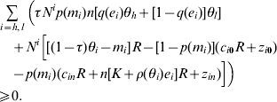
With quasi-linear utility, marginal utility from working age consumption will be unity across individuals. Since redistribution will not affect welfare as long as the condition for marginal utility is met, a continuum of first-best allocations exists.
First, equalizing marginal utility across states in old age implies that

has to hold in any social optimum, where the subscript denotes the type of the individual and the number of children, and the superscript their productivity. Hence, a perfect old age consumption insurance has to exist.
Socially optimal investment in education then balances the cost of education against all benefits accruing to the parent generation

In the optimum, the type-specific cost of increasing education for the n children in the family by one unit, nρ(θi), is equal to the sum of the expected non-monetary payoff for the parents, q′(e i)[ψ(θh) −ψ(θl)], and the present value of the expected additional transfers from these children to the public pension system, q′(e i)[τn(θh−θl)/R]. Since q is strictly concave, the smaller price of education for more productive parents implies that these parents have to invest more into their children's human capital, e h>e l. Comparing the conditions for the two types of parents yields
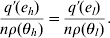
In other words, the marginal impact of investing an additional dollar into education of a child has to be the same for low productivity parents and high productivity parents.
Turning to the fertility investment decision, the optimality condition is
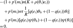
Increasing the fertility investment by one unit yields additional expected costs of raising and educating children of p′(m i)n(K+ρ(θi)e i). The present value of the expected pension contributions of the potential children increases by p′(m i)nτ[q(e i)θh+(1−q(e i))θl]/R. In addition, the expected non-monetary payoff to potential parents rises by p′(m i)[q(e i)ψ(θh)+(1−q(e i))ψ(θl)].
Note that the difference between expected social benefits of n children, (nτ/R)[q(e i)]θh+(1−q(e i))θl]+[q(e i)ψ(θh)+(1−q(e i))ψ(θl)], and their social costs, n(K+ρ(θi)e i), must be higher for high productivity parents in the social optimum. This property would already hold if high productivity parents choose the same human capital investment as low productivity parents. When high productivity parents invest more into their children's human capital, the social planner achieves an even higher difference between expected benefits and costs. The higher net benefit of children implies that high productivity individuals invest more in fertility in the social optimum, leading to a higher expected number of children.
The outcome that productive parents have more children on average and invest more per child reflects their advantage in human capital production. This result need not hold if opportunity costs were taken into account such that, for example, lifetime labor supply has to be reduced with a higher number of children irrespective of the mother's productivity.
In a laissez-faire economy with a lump-sum pension, we have two deviations from the social optimum. As individuals neglect the positive fiscal externalities, they invest too little in both the quantity and the quality of human capital. If this problem is solved by assigning all contributions of a child to her mother, we will no longer have the same level of old age consumption irrespective of her children's productivity.
5 Second-best pension schemes
We proceed by characterizing second-best allocations, where it is taken into account that the government does not observe the individual's decisions on fertility investment, educational effort per child, and saving. It will turn out that introducing the moral hazard aspect involves a tradeoff between the desire to provide old age consumption insurance and the necessity to set incentives for investment in fertility and education. Transfers to pensioners can be made contingent on the observable outcomes of the investment decisions, that is on the number of children and on their wage rates. Furthermore, we confine ourselves to linear PAYG schemes. At the end of the section, we will argue that this assumption is not really restrictive.
The government's problem is to maximize aggregate expected utility (11) with respect to the pension parameters α, β, γ, δ subject to the individual's first-order conditions for optimum savings, education effort, and fertility investment, being represented by demand functions, and the pension budget constraint
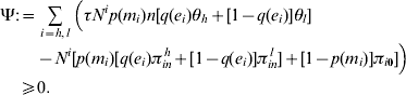
The first-order conditions for an interior solution are

where λ is the Lagrange multiplier of the PAYG budget constraint. The envelope theorem implies that all terms vanish except for the direct impacts of parameter φ changes through the pension scheme and the repercussions in the pension budget restriction. Raising a pension parameter increases welfare through higher values of old age consumption. At the optimum, this increase will be equal to the shadow value of the resulting marginal budget deficit. The revenue side of the pension budget changes due to a varying number and quality of contributors. Expenditures change directly and through the stochastic consequences of the behavioral responses in the parent generation.
For the contribution-related pension parameter α and the flat pension δ, the first-order conditions boil down to λ=1/R. The two parameters are to some extent indeterminate because redistribution is neutral with respect to welfare.
Using λ=1/R, the first-order condition for the fertility-related pension parameter β is
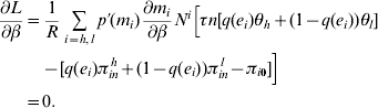
With an increasing β, the positive impact on welfare through rising old age consumption levels is perfectly offset by a higher social security deficit at given fertility levels. The net impacts arise through increasing fertility. This raises both the number of future contributors and the number of individuals receiving pension components for parents. Condition (19) shows that at the second-best optimum parents of at least one productivity group i will receive aggregate excess pension benefits N ip(m i)[q(e i)πinh+(1−q(e i))πinl−πi0] amounting to at least the expected total contributions of their children, N ip(m i)τn[q(e i)θh+(1−q(e i))θl]. If this holds for both groups, childless individuals do not receive any benefit. Inserting the pension formulas into (19) and isolating β yields
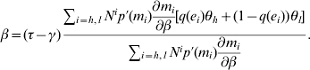
Hence, if γ is equal to its maximum value, τ, the fertility-related pension parameter β must be zero. If γ is smaller than τ, β will be positive. The fertility-related pension element is a substitute for children's contributions being directly assigned to their parents.
For the pension part contingent on the own children's contributions, the first-order condition is
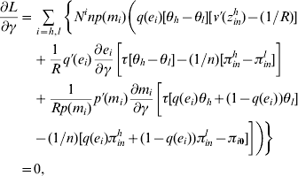
where λ=1/R and (8) have been used. The first line of equation (21) can be interpreted as follows. Increasing the pension contingent on own children's contributions raises welfare through more old age consumption of parents, but also implies a deficit in the pension scheme. Note that perfect consumption smoothing across all states is impossible with γ>0. Recalling that v′(z inh)−(1/R)<0 holds if γ>0 according to (8), the net direct effect of increasing γ on welfare will be negative. In addition, as shown in the second line, with a rising education investment, we will have more high productivity individuals among the contributors and more pensioners with children receiving the higher benefit. Finally, as fertility is also increased, both the total number of contributors and the number of individuals claiming parental benefits will rise.
Inserting the pension formulas, the equation (21) can be written as
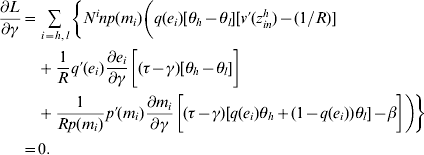
Proposition 1 describes the two main features of second-best schemes.
Proposition 1
Any second-best linear PAYG scheme is characterized (i) by partial assignment of children's contributions to their parents (i.e. 0<γ<τ), and (ii) by a strictly positive fertility-related component (i.e. β>0).
Proof
See Appendix D. □
The proposition is easily understood. If parents would receive the full contribution of their children, there is no role for a purely fertility-related component. However, with such a perfect internalization, old age consumption smoothing across different states according to the children's productivity is not achieved. Utility can therefore be increased by a reduction of the pension contingent on own children's contribution and using these resources in a different fashion. Furthermore, if we do not have a full assignment of children's contributions to their parents, it always pays to introduce purely fertility-related pensions. This result turns out since the externality is still present and fertility-related pensions do not increase the old age consumption risk among parents. Last, it is not optimal to exclusively rely on fertility-related pensions. The obvious reason is that the positive externalities of investing in human capital are not properly addressed by such a policy.
An obvious objection against our analysis lies in the restricted set of solutions by imposing a parametric linear structure of the pension formula. As an alternative, πi0, πinh, and πinl for i=h, l may be taken as control variables, where a non-linear second-best pension system can be derived. We omit the calculation here since the optimum non-linear scheme turns out to be similar to the linear PAYG scheme. We obtain λ=1/R and N hπh0+N lπl0=0. If pensions cannot become negative, this condition means that childless individuals will not receive any pension. Furthermore, parents of high productivity children should receive higher pensions than parents of low productivity children (i.e. πinh>πinl). Finally, they should receive less than their children contribute (i.e. πinj<τθjn) provided that πh0=πj0=0.
6 Conclusions
Incorporating the fiscal externalities of investing in the quantity and quality of human capital arising through the pension scheme requires encouraging both fertility and education. We have restricted our attention to modifications of the pension formula. In a deterministic environment, a perfect internalization would be achieved by assigning all contributions of a child to her parent. Such a policy may still be associated with underinvestment in education if parents do not take the benefits accruing to their children fully into account. Our analysis has ignored these relations between parents and their children and focuses on the impacts of uncertain investment outcomes instead. Due to the uncertainty of the investment into education, the optimum scheme requires that parents receive less than the total contributions of their children. Insurance against having less productive children is provided by a purely fertility-related component in the pension formula.
Endogenizing labor supply would certainly be an interesting extension of the current analysis. Any type of fertility-related benefit financed by payroll taxes tends to distort labor supply. Moreover, labor supply decisions will be associated with a positive fiscal externality working through the pension scheme. Individuals will not take into account the positive impacts on pensioners at a given social security contribution rate when considering an increase in their labor supply. Recognizing the results in similar frameworks with endogenous labor supply (Fenge and Meier, Reference Fenge and Meier2005 and Reference Fenge and Meier2008), we expect that such considerations drive up the share of contribution-related pensions, while both types of fertility-related pensions continue to exist.
If alternative instruments are used, the purely fertility-related component of the incentive payment will typically be a family allowance, where the amount is not contingent on parental income. Replacing the contributions paid by children requires payments that depend on revealed ability of the child. An example of such a benefit is a scholarship being paid for advanced students. Since high productivity parents will invest more per child, they will on average receive more of these benefits. It is not obvious whether alternative policy instruments can work better when dealing with the fiscal externality problem. In principle, in an environment with fluctuations in productivity over the life-cycle, tying benefits to a signal is warranted that exhibits the closest correlation with the parents' educational efforts.
Finally, there is no rationale for providing insurance against having no children in our analysis. This problem does not arise here, as the quasi-linear utility function ensures that expected marginal utility of consumption will not be affected by the number of children. For the same reason, the result of Cremer et al. (Reference Cremer, Gahvari and Pestieau2006a) that optimum PAYG pension schemes with stochastic fertility will exhibit strictly positive pensions for childless individuals is not replicated in our model. In a more general framework, the consequences of designing such an element of insurance will probably be ambiguous. Even comparing child care costs to the expected present value of excess pension benefits for parents does not indicate the direction of income redistribution across states when the existence of children affects the marginal utility of consumption. The clear tendency however is that higher child care costs call for even stronger subsidization of families. On the other hand, a more generous pension scheme associated with high benefits for families may require some compensation for those who remain childless.
Appendix
Proof of Lemma 1
The Jacobian of the system of equations (7)–(10) is
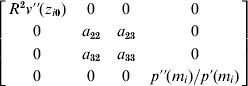
with


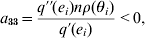
where (7)–(10) are already taken into account.
Ignoring the boundary case that only necessary conditions hold, the determinant of the Jacobian has to be positive in order to satisfy all sufficient second-order conditions:

which requires a 22a 33−a 23a 32>0.
The vector of derivatives of the equations (7)–(10) with respect to δ is

Applying the implicit function theorem then yields

In a perfectly analogous fashion, it follows that

The vector of derivatives of the equations (7)–(19) with respect to β is

Applying the implicit function theorem then yields

□
Proof of Lemma 2
The vector of derivatives of the equations (7)–(10) with respect to γ is
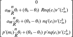
Applying the implicit function theorem then yields ∂s i0/∂γ=0
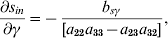
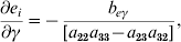

with a 22a 33−a 23a 32>0 due to the strict concavity of the household's optimization problem, and
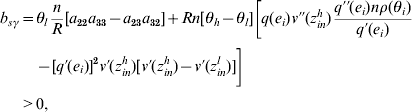
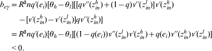
□
Proof of Lemma 3
The vector of derivatives of the equations (7)–(10) with respect to θ is
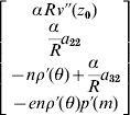
Applying the implicit function theorem then yields ∂s 0/∂θ=−α/R
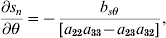
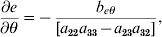
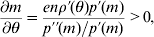
with a 22a 33−a 23a 32>0 due to the strict concavity of the household's optimization problem, and


□
Proof of Proposition 1
Note that γ=τ will be associated with β=0 according to (19). In this event, it follows that  , since v′(z inh)−(1/R)<0. Hence, γ<τ must hold for the optimum scheme.
With γ<τ, the inequality  holds at β=0. Therefore, the optimum scheme requires β>0.
Consider now the boundary γ=0, where β is chosen so as to satisfy (19). Then we have v′(z inh)−(1/R)=0 and, according to the Lemmas 1 and 2, 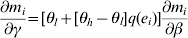 . Taking (20) into account, we finally get
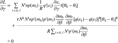
□
at γ=0. Thus, γ>0 must be a property of the optimum scheme.