1 Introduction
The growth in computing for scientific, engineering and social applications has long been a driver of advances in methods for numerical optimization. The development of derivative-free optimization methods – those methods that do not require the availability of derivatives – has especially been driven by the need to optimize increasingly complex and diverse problems. One of the earliest calculations on MANIAC,Footnote 1 an early computer based on the von Neumann architecture, was the approximate solution of a six-dimensional non-linear least-squares problem using a derivative-free coordinate search (Fermi and Metropolis Reference Fermi and Metropolis1952). Today, derivative-free methods are used routinely, for example by Google (Golovin et al. Reference Golovin, Solnik, Moitra, Kochanski, Karro and Sculley2017), for the automation and tuning needed in the artificial intelligence era.
In this paper we survey methods for derivative-free optimization and key results for their analysis. Since the field – also referred to as black-box optimization, gradient-free optimization, optimization without derivatives, simulation-based optimization and zeroth-order optimization – is now far too expansive for a single survey, we focus on methods for local optimization of continuous-valued, single-objective problems. Although Section 8 illustrates further connections, here we mark the following notable omissions.
∙ We focus on methods that seek a local minimizer. Despite users understandably desiring the best possible solution, the problem of global optimization raises innumerably more mathematical and computational challenges than do the methods presented here. We instead point to the survey by Neumaier (Reference Neumaier2004), which importantly addresses general constraints, and to the textbook by Forrester, Sobester and Keane (Reference Forrester, Sobester and Keane2008), which lays a foundation for global surrogate modelling.
∙ Multi-objective optimization and optimization in the presence of discrete variables are similarly popular tasks among users. Such problems possess fundamental challenges as well as differences from the methods presented here.
∙ In focusing on methods, we cannot do justice to the application problems that have driven the development of derivative-free methods and benefited from implementations of these methods. The recent textbook by Audet and Hare (Reference Audet and Hare2017) contains a number of examples and references to applications; Rios and Sahinidis (Reference Rios and Sahinidis2013) and Auger et al. (Reference Auger, Hansen, Perez Zerpa, Ros, Schoenauer and Vahrenhold2009) both reference a diverse set of implementations. At the persistent page

we intend to link all works that cite the entries in our bibliography and those that cite this survey; we hope this will provide a coarse, but dynamic, catalogue for the reader interested in potential uses of these methods.

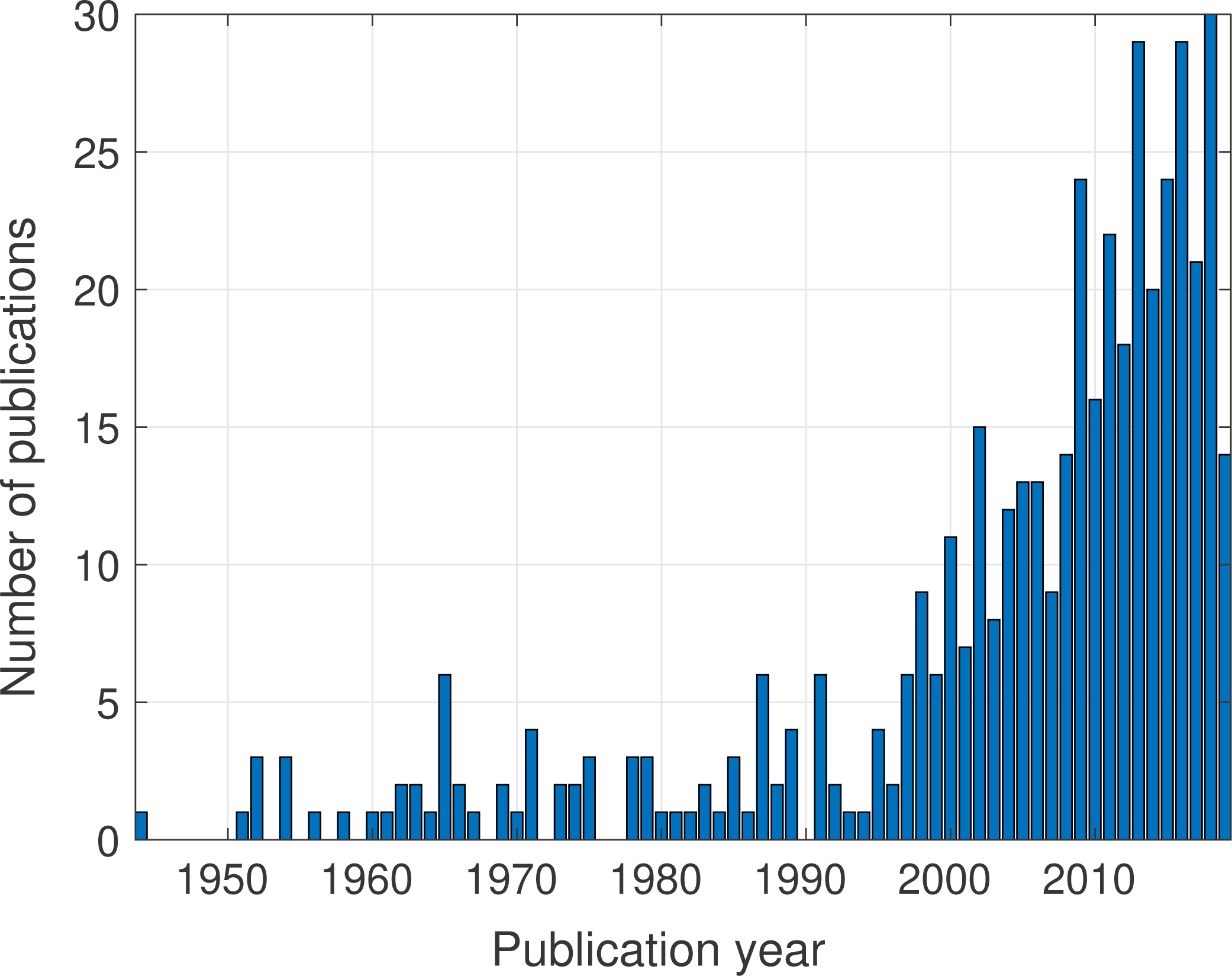
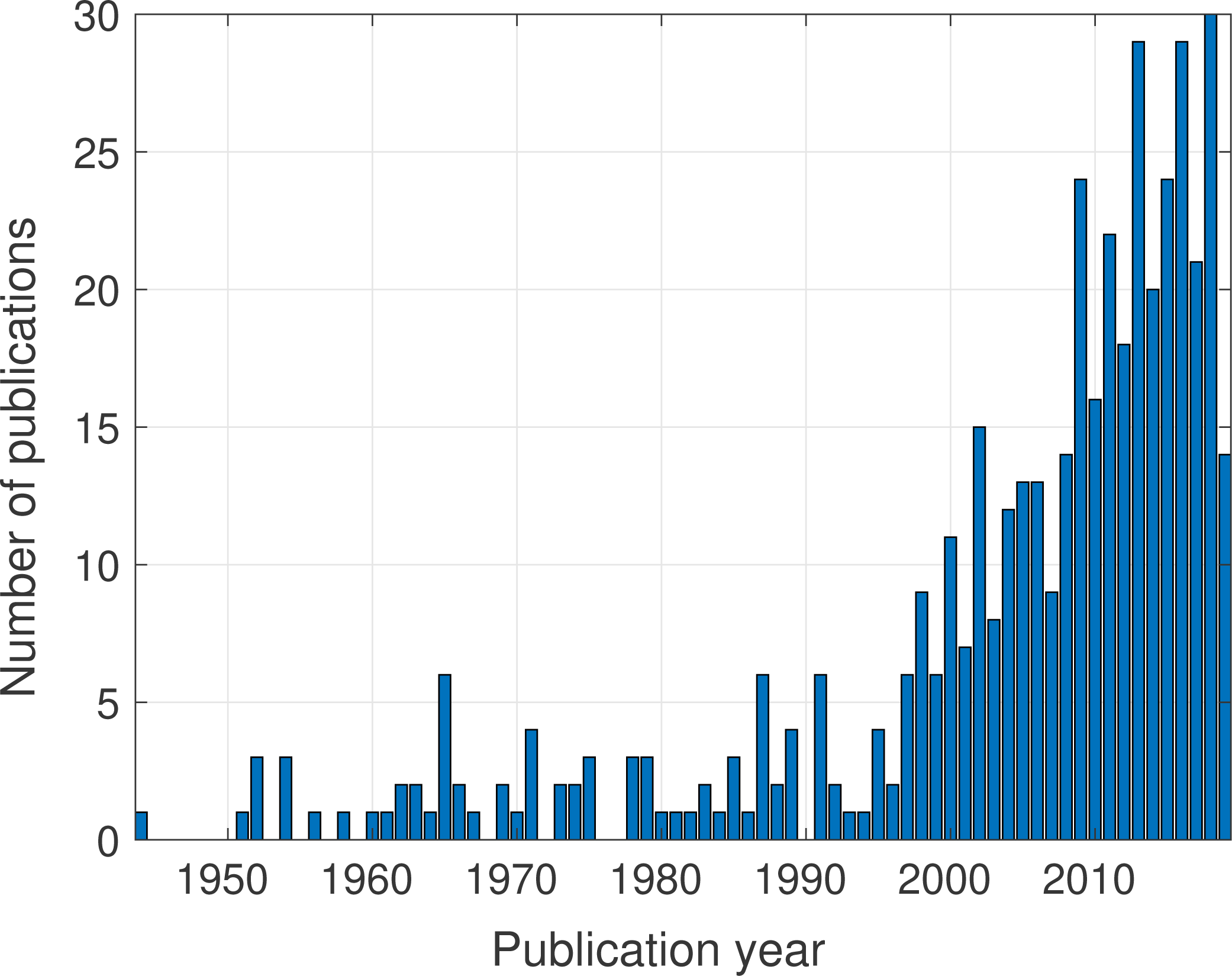
Given these limitations, we particularly note the intersection with the foundational books by Kelley (Reference Kelley1999b ) and Conn, Scheinberg and Vicente (Reference Conn, Scheinberg and Vicente2009b ). Our intent is to highlight recent developments in, and the evolution of, derivative-free optimization methods. Figure 1.1 summarizes our bias; over half of the references in this survey are from the past ten years.
Histogram of the references cited in the bibliography.
Many of the fundamental inspirations for the methods discussed in this survey are detailed to a lesser extent. We note in particular the activity in the United Kingdom in the 1960s (see e.g. the works by Rosenbrock Reference Rosenbrock1960, Powell Reference Powell1964, Nelder and Mead Reference Nelder and Mead1965, Fletcher Reference Fletcher1965 and Box Reference Box1966, and the later exposition and expansion by Brent Reference Brent1973) and the Soviet Union (as evidenced by Rastrigin Reference Rastrigin1963, Matyas Reference Matyas1965, Karmanov Reference Karmanov1974, Polyak Reference Polyak1987 and others). In addition to those mentioned later, we single out the work of Powell (Reference Powell1975), Wright (Reference Wright, Griffiths and Watson1995), Davis (Reference Davis2005) and Leyffer (Reference Leyffer2015) for insight into some of these early pioneers.
With our focus clear, we turn our attention to the deterministic optimization problem
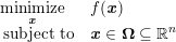
and the stochastic optimization problem
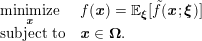
Although important exceptions are noted throughout this survey, the majority of the methods discussed assume that the objective function
 $f$
in (DET) and (STOCH) is differentiable. This assumption may cause readers to pause (and some readers may never resume). The methods considered here do not necessarily address non-smooth optimization; instead they address problems where a (sub)gradient of the objective
 $f$
or a constraint function defining
 $\boldsymbol{\unicode[STIX]{x1D6FA}}$
is not available to the optimization method. Note that similar naming confusion has existed in non-smooth optimization, as evidenced by the introduction of Lemarechal and Mifflin (Reference Lemarechal and Mifflin1978):
This workshop was held under the name Nondifferentiable Optimization, but it has been recognized that this is misleading, because it suggests ‘optimization without derivatives’.
1.1 Alternatives to derivative-free optimization methods
Derivative-free optimization methods are sometimes employed for convenience rather than by necessity. Since the decision to use a derivative-free method typically limits the performance – in terms of accuracy, expense or problem size – relative to what one might expect from gradient-based optimization methods, we first mention alternatives to using derivative-free methods.
The design of derivative-free optimization methods is informed by the alternatives of algorithmic and numerical differentiation. For the former, the purpose seems clear: since the methods use only function values, they apply even in cases when one cannot produce a computer code for the function’s derivative. Similarly, derivative-free optimization methods should be designed in order to outperform (typically measured in terms of the number of function evaluations) gradient-based optimization methods that employ numerical differentiation.
1.1.1 Algorithmic differentiation
Algorithmic differentiationFootnote 2 (AD) is a means of generating derivatives of mathematical functions that are expressed in computer code (Griewank Reference Griewank2003, Griewank and Walther Reference Griewank and Walther2008). The forward mode of AD may be viewed as performing differentiation of elementary mathematical operations in each line of source code by means of the chain rule, while the reverse mode may be seen as traversing the resulting computational graph in reverse order.
Algorithmic differentiation has the benefit of automatically exploiting function structure, such as partial separability or other sparsity, and the corresponding ability of producing a derivative code whose computational cost is comparable to the cost of evaluating the function code itself.
AD has seen significant adoption and advances in the past decade (Forth et al. Reference Forth, Hovland, Phipps, Utke and Walther2012). Tools for algorithmic differentiation cover a growing set of compiled and interpreted languages, with an evolving list summarized on the community portal at

Progress has also been made on algorithmic differentiation of piecewise smooth functions, such as those with breakpoints resulting from absolute values or conditionals in a code; see, for example, Griewank, Walther, Fiege and Bosse (Reference Griewank, Walther, Fiege and Bosse2016). The machine learning renaissance has also fuelled demand and interest in AD, driven in large part by the success of algorithmic differentiation in backpropagation (Baydin, Pearlmutter, Radul and Siskind Reference Baydin, Pearlmutter, Radul and Siskind2018).
1.1.2 Numerical differentiation
Another alternative to derivative-free methods is to estimate the derivative of
 $f$
by numerical differentiation and then to use the estimates in a derivative-based method. This approach has the benefit that only zeroth-order information (i.e. the function value) is needed; however, depending on the derivative-based method used, the quality of the derivative estimate may be a limiting factor. Here we remark that for the finite-precision (or even fixed-precision) functions encountered in scientific applications, finite-difference estimates of derivatives may be sufficient for many purposes; see Section 2.3.1.
When numerical derivative estimates are used, the optimization method must tolerate inexactness in the derivatives. Such methods have been classically studied for both non-linear equations and unconstrained optimization; see, for example, the works of Powell (Reference Powell1965), Brown and Dennis, Jr (Reference Brown and Dennis1971) and Mifflin (Reference Mifflin1975) and the references therein. Numerical derivatives continue to be employed by recent methods (see e.g. the works of Cartis, Gould and Toint Reference Cartis, Gould and Toint2012 and Berahas, Byrd and Nocedal Reference Berahas, Byrd and Nocedal2019). Use in practice is typically determined by whether the limit on the derivative accuracy and the expense in terms of function evaluations are acceptable.
1.2 Organization of the paper
This paper is organized principally by problem class: unconstrained domain (Sections 2 and 3), convex objective (Section 4), structured objective (Section 5), stochastic optimization (Section 6) and constrained domain (Section 7).
Section 2 presents deterministic methods for solving (DET) when
 $\boldsymbol{\unicode[STIX]{x1D6FA}}=\mathbb{R}^{n}$
. The section is split between direct-search methods and model-based methods, although the lines between these are increasingly blurred; see, for example, Conn and Le Digabel (Reference Conn and Le Digabel2013), Custódio, Rocha and Vicente (Reference Custódio, Rocha and Vicente2009), Gramacy and Le Digabel (Reference Gramacy and Le Digabel2015) and Gratton, Royer and Vicente (Reference Gratton, Royer and Vicente2016). Direct-search methods are summarized in far greater detail by Kolda, Lewis and Torczon (Reference Kolda, Lewis and Torczon2003) and Kelley (Reference Kelley1999b
), and in the more recent survey by Audet (Reference Audet, Pardalos and Rassias2014). Model-based methods that employ trust regions are given full treatment by Conn et al. (Reference Conn, Scheinberg and Vicente2009b
), and those that employ stencils are detailed by Kelley (Reference Kelley2011).
In Section 3 we review randomized methods for solving (DET) when
 $\boldsymbol{\unicode[STIX]{x1D6FA}}=\mathbb{R}^{n}$
. These methods are often variants of the deterministic methods in Section 2 but require additional notation to capture the resulting stochasticity; the analysis of these methods can also deviate significantly from their deterministic counterparts.
In Section 4 we discuss derivative-free methods intended primarily for convex optimization. We make this delineation because such methods have distinct lines of analysis and can often solve considerably higher-dimensional problems than can general methods for non-convex derivative-free optimization.
In Section 5 we survey methods that address particular structure in the objective
 $f$
in (DET). Examples of such structure include non-linear least-squares objectives, composite non-smooth objectives and partially separable objectives.
In Section 6 we address derivative-free stochastic optimization, that is, when methods have access only to a stochastic realization of a function in pursuit of solving (STOCH). This topic is increasingly intertwined with simulation optimization and Monte Carlo-based optimization; for these areas we refer to the surveys by Homem-de-Mello and Bayraksan (Reference Homem-de-Mello and Bayraksan2014), Fu, Glover and April (Reference Fu, Glover and April2005), Amaran, Sahinidis, Sharda and Bury (Reference Amaran, Sahinidis, Sharda and Bury2015) and Kim, Pasupathy and Henderson (Reference Kim, Pasupathy, Henderson and Fu2015).
Section 7 presents methods for deterministic optimization problems with constraints (i.e.
 $\boldsymbol{\unicode[STIX]{x1D6FA}}\subset \mathbb{R}^{n}$
). Although many of these methods rely on the foundations laid in Sections 2 and 3, we highlight particular difficulties associated with constrained derivative-free optimization.
In Section 8 we briefly highlight related problem areas (including global and multi-objective derivative-free optimization), methods and other implementation considerations.
2 Deterministic methods for deterministic objectives
We now address deterministic methods for solving (DET). We discuss direct-search methods in Section 2.1, model-based methods in Section 2.2 and other methods in Section 2.3. At a coarse level, direct-search methods use comparisons of function values to directly determine candidate points, whereas model-based methods use a surrogate of
 $f$
to determine candidate points. Naturally, some hybrid methods incorporate ideas from both model-based and direct-search methods and may not be so easily categorized. An early survey of direct-search and model-based methods is given in Powell (Reference Powell1998a
).
2.1 Direct-search methods
Although Hooke and Jeeves (Reference Hooke and Jeeves1961) are credited with originating the term ‘direct search’, there is no agreed-upon definition of what constitutes a direct-search method. We follow the convention of Wright (Reference Wright, Griffiths and Watson1995), wherein a direct-search method is a method that uses only function values and ‘does not “in its heart” develop an approximate gradient’.
We first discuss simplex methods, including the Nelder–Mead method – perhaps the most widely used direct-search method. We follow this discussion with a presentation of directional direct-search methods; hybrid direct-search methods are discussed in Section 2.3. (The global direct-search method DIRECT is discussed in Section 8.3.)
2.1.1 Simplex methods
Simplex methods (not to be confused with Dantzig’s simplex method for linear programming) move and manipulate a collection of
 $n+1$
affinely independent points (i.e. the vertices of a simplex in
 $\mathbb{R}^{n}$
) when solving (DET). The method of Spendley, Hext and Himsworth (Reference Spendley, Hext and Himsworth1962) involves either taking the point in the simplex with the largest function value and reflecting it through the hyperplane defined by the remaining
 $n$
points or moving the
 $n$
worst points toward the best vertex of the simplex. In this manner, the geometry of all simplices remains the same as that of the starting simplex. (That is, all simplices are similar in the geometric sense.)
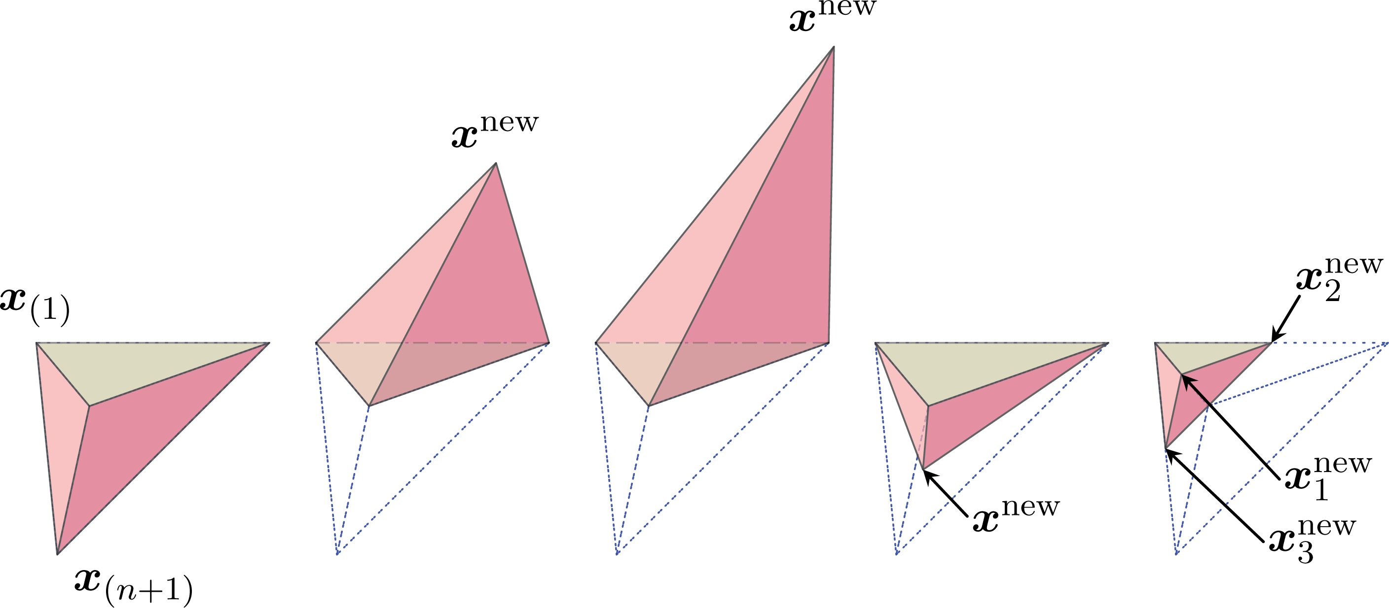
Nelder and Mead (Reference Nelder and Mead1965) extend the possible simplex operations, as shown in Figure 2.1, by allowing the ‘expansion’ and ‘contraction’ operations in addition to the ‘reflection’ and ‘shrink’ operations of Spendley et al. (Reference Spendley, Hext and Himsworth1962). These operations enable the Nelder–Mead simplex method to distort the simplex in order to account for possible curvature present in the objective function.
Nelder and Mead (Reference Nelder and Mead1965) propose stopping further function evaluations when the standard error of the function values at the simplex vertices is small. Others, Woods (Reference Woods1985) for example, propose stopping when the size of the simplex’s longest side incident to the best simplex vertex is small.
Primary Nelder–Mead simplex operations: original simplex, reflection, expansion, inner contraction, and shrink.

Nelder–Mead is an incredibly popular method, in no small part due to its inclusion in Numerical Recipes (Press, Teukolsky, Vetterling and Flannery Reference Press, Teukolsky, Vetterling and Flannery2007), which has been cited over
 $125\,000$
times and no doubt used many times more. The method (as implemented by Lagarias, Poonen and Wright Reference Lagarias, Poonen and Wright2012) is also the algorithm underlying fminsearch in MATLAB. Benchmarking studies highlight Nelder–Mead performance in practice (Moré and Wild Reference Moré and Wild2009, Rios and Sahinidis Reference Rios and Sahinidis2013).
The method’s popularity from its inception was not diminished by the lack of theoretical results proving its ability to identify stationary points. Woods (Reference Woods1985) presents a non-convex, two-dimensional function where Nelder–Mead converges to a non-stationary point (where the function’s Hessian is singular). Furthermore, McKinnon (Reference McKinnon1998) presents a class of thrice-continuously differentiable, strictly convex functions on
 $\mathbb{R}^{2}$
where the Nelder–Mead simplex fails to converge to the lone stationary point. The only operation that Nelder–Mead performs on this relatively routine function is repeated ‘inner contraction’ of the initial simplex.
Researchers have continued to develop convergence results for modified or limited versions of Nelder–Mead. Kelley (Reference Kelley1999a ) addresses Nelder–Mead’s theoretical deficiencies by restarting the method when the objective decrease on consecutive iterations is not larger than a multiple of the simplex gradient norm. Such restarts do not ensure that Nelder–Mead will converge: Kelley (Reference Kelley1999a ) shows an example of such behaviour. Price, Coope and Byatt (Reference Price, Coope and Byatt2002) embed Nelder–Mead in a different (convergent) algorithm using positive spanning sets. Nazareth and Tseng (Reference Nazareth and Tseng2002) propose a clever, though perhaps superfluous, variant that connects Nelder–Mead to golden-section search.
Lagarias, Reeds, Wright and Wright (Reference Lagarias, Reeds, Wright and Wright1998) show that Nelder–Mead (with appropriately chosen reflection and expansion coefficients) converges to the global minimizer of strictly convex functions when
 $n=1$
. Gao and Han (Reference Gao and Han2012) show that the contraction and expansion steps of Nelder–Mead satisfy a descent condition on uniformly convex functions. Lagarias, Poonen and Wright (Reference Lagarias, Poonen and Wright2012) show that a restricted version of the Nelder–Mead method – one that does not allow an expansion step – can converge to minimizers of any twice-continuously differentiable function with a positive-definite Hessian and bounded level sets. (Note that the class of functions from McKinnon (Reference McKinnon1998) have singular Hessians at only one point – their minimizers – and not at the point to which the simplex vertices are converging.)
The simplex method of Rykov (Reference Rykov1980) includes ideas from model-based methods. Rykov varies the number of reflected vertices from iteration to iteration, following one of three rules that depend on the function value at the simplex centroid
 $\boldsymbol{x}_{c}$
. Rykov considers both evaluating
 $f$
at the centroid and approximating
 $f$
at the centroid using the values of
 $f$
at the vertex. The non-reflected vertices are also moved in parallel with the reflected subset of vertices. In general, the number of reflected vertices is chosen so that
 $\boldsymbol{x}_{c}$
moves in a direction closest to
 $-\unicode[STIX]{x1D6FB}f(\boldsymbol{x}_{c})$
. This, along with a test of sufficient decrease in
 $f$
, ensures convergence of the modified simplex method to a minimizer of convex, continuously differentiable functions with bounded level sets and Lipschitz-bounded gradients. (The sufficient-decrease condition is also shown to be efficient for the classical Nelder–Mead algorithm.)
Tseng (Reference Tseng1999) proposes a modified simplex method that keeps the
 $b_{k}$
best simplex vertices on a given iteration
 $k$
and uses them to reflect the remaining vertices. Their method prescribes that ‘the rays emanating from the reflected vertices toward the
 $b_{k}$
best vertices should contain, in their convex hull, the rays emanating from a weighted centroid of the
 $b_{k}$
best vertices toward the to-be-reflected vertices’. Their method also includes a fortified descent condition that is stronger than common sufficient-decrease conditions. If
 $f$
is continuously differentiable and bounded below and
 $b_{k}$
is fixed for all iterations, Tseng (Reference Tseng1999) prove that every cluster point of the sequence of candidate points generated by their method is a stationary point.
Bűrmen, Puhan and Tuma (Reference Bűrmen, Puhan and Tuma2006) propose a convergent version of a simplex method that does not require a sufficient descent condition to be satisfied. Instead, they ensure that evaluated points lie on a grid of points, and they show that this grid will be refined as the method proceeds.
2.1.2 Directional direct-search methods
Broadly speaking, each iteration of a directional direct-search (DDS) method generates a finite set of points near the current point
 $\boldsymbol{x}_{k}$
; these poll points are generated by taking
 $\boldsymbol{x}_{k}$
and adding terms of the form
 $\unicode[STIX]{x1D6FC}_{k}\boldsymbol{d}$
, where
 $\unicode[STIX]{x1D6FC}_{k}$
is a positive step size and
 $\boldsymbol{d}$
is an element from a finite set of directions
 $\boldsymbol{D}_{k}$
. Kolda et al. (Reference Kolda, Lewis and Torczon2003) propose the term generating set search methods to encapsulate this class of methods.Footnote
3
The objective function
 $f$
is then evaluated at all or some of the poll points, and
 $\boldsymbol{x}_{k+1}$
is selected to be some poll point that produces a (sufficient) decrease in the objective and the step size is possibly increased. If no poll point provides a sufficient decrease,
 $\boldsymbol{x}_{k+1}$
is set to
 $\boldsymbol{x}_{k}$
and the step size is decreased. In either case, the set of directions
 $\boldsymbol{D}_{k}$
can (but need not) be modified to obtain
 $\boldsymbol{D}_{k+1}$
.
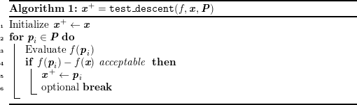
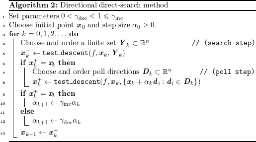
A general DDS method is provided in Algorithm 2, which includes a search step where
 $f$
is evaluated at any finite set of points
 $\boldsymbol{Y}_{k}$
, including
 $\boldsymbol{Y}_{k}=\emptyset$
. The search step allows one to (potentially) improve the performance of Algorithm 2. For example, points could be randomly sampled during the search step from the domain in the hope of finding a better local minimum, or a person running the algorithm may have problem-specific knowledge that can generate candidate points given the observed history of evaluated points and their function values. While the search step allows for this insertion of such heuristics, rigorous convergence results are driven by the more disciplined poll step. When testing for objective decrease in Algorithm 1, one can stop evaluating points in
 $\boldsymbol{P}$
(line 6) as soon as the first point is identified where there is (sufficient) decrease in
 $f$
. In this case, the polling (or search) step is considered opportunistic.
DDS methods are largely distinguished by how they generate the set of poll directions
 $\boldsymbol{D}_{k}$
at line 7of Algorithm 2. Perhaps the first approach is coordinate search, in which the poll directions are defined as
 $\boldsymbol{D}_{k}=\{\pm \boldsymbol{e}_{i}:i=1,2,\ldots ,n\}$
, where
 $\boldsymbol{e}_{i}$
denotes the
 $i$
th elementary basis vector (i.e. column
 $i$
of the identity matrix in
 $n$
dimensions). The first known description of coordinate search appears in the work of Fermi and Metropolis (Reference Fermi and Metropolis1952) where the smallest positive integer
 $l$
is sought such that
 $f(\boldsymbol{x}_{k}+l\unicode[STIX]{x1D6FC}\boldsymbol{e}_{1}/2)>f(\boldsymbol{x}_{k}+(l-1)\unicode[STIX]{x1D6FC}\boldsymbol{e}_{1}/2)$
. If an increase in
 $f$
is observed at
 $\boldsymbol{e}_{1}/2$
then
 $-\boldsymbol{e}_{1}/2$
is considered. After such an integer
 $l$
is identified for the first coordinate direction,
 $\boldsymbol{x}_{k}$
is updated to
 $\boldsymbol{x}_{k}\pm l\boldsymbol{e}_{1}/2$
and the second coordinate direction is considered. If
 $\boldsymbol{x}_{k}$
is unchanged after cycling through all coordinate directions, then the method is repeated but with
 $\pm \boldsymbol{e}_{i}/2$
replaced with
 $\pm \boldsymbol{e}_{i}/16$
, terminating when no improvement is observed for this smaller
 $\unicode[STIX]{x1D6FC}$
. In terms of Algorithm 2the search set
 $\boldsymbol{Y}_{k}=\emptyset$
at line 4, and the descent test at line 4of Algorithm 1merely tests for simple decrease, that is,
 $f(\boldsymbol{p}_{i})-f(\boldsymbol{x})<0$
. Other versions of acceptability in line 4of Algorithm 1are employed by methods discussed later.
Proofs that DDS methods converge first appeared in the works of Céa (Reference Céa1971) and Yu (Reference Yu1979), although both require the sequence of step-size parameters to be non-increasing. Lewis, Torczon and Trosset (Reference Lewis, Torczon and Trosset2000) attribute the first global convergence proof for coordinate search to Polak (Reference Polak1971, p. 43). In turn, Polak cites the ‘method of local variation’ of Banichuk, Petrov and Chernous’ko (Reference Banichuk, Petrov and Chernous’ko1966); although Banichuk et al. (Reference Banichuk, Petrov and Chernous’ko1966) do develop parts of a convergence proof, they state in Remark 1 that ‘the question of the strict formulation of the general sufficient conditions for convergence of the algorithm to a minimum remains open’.
Typical convergence results for DDS require that the set
 $\boldsymbol{D}_{k}$
is a positive spanning set (PSS) for the domain
 $\boldsymbol{\unicode[STIX]{x1D6FA}}$
; that is, any point
 $\boldsymbol{x}\in \boldsymbol{\unicode[STIX]{x1D6FA}}$
can be written as
 $$\begin{eqnarray}\displaystyle \boldsymbol{x}=\mathop{\sum }_{i=1}^{|\boldsymbol{D}_{k}|}\unicode[STIX]{x1D706}_{i}\boldsymbol{d}_{i}, & & \displaystyle \nonumber\end{eqnarray}$$
where
 $\boldsymbol{d}_{i}\in \boldsymbol{D}_{k}$
and
 $\unicode[STIX]{x1D706}_{i}\geq 0$
for all
 $i$
. Some of the first discussions of properties of positive spanning sets were presented by Davis (Reference Davis1954) and McKinney (Reference McKinney1962), but recent treatments have also appeared in Regis (Reference Regis2016). In addition to requiring positive spanning sets during the poll step, earlier DDS convergence results depended on
 $f$
being continuously differentiable. When
 $f$
is non-smooth, no descent direction is guaranteed for these early DDS methods, even when the step size is arbitrarily small. See, for example, the modification of the Dennis–Woods (Dennis, Jr and Woods Reference Dennis, Woods and Wouk1987) function by Kolda et al. (Reference Kolda, Lewis and Torczon2003, Figure 6.2) and a discussion of why coordinate-search methods (for example) will not move when started at a point of non-differentiability; moreover, when started at differentiable points, coordinate-search methods tend to converge to a point that is not (Clarke) stationary.
The pattern-search method of Torczon (Reference Torczon1991) revived interest in direct-search methods. The method therein contains ideas from both DDS and simplex methods. Given a simplex defined by
 $\boldsymbol{x}_{k},\boldsymbol{y}_{1},\ldots ,\boldsymbol{y}_{n}$
(where
 $\boldsymbol{x}_{k}$
is the simplex vertex with smallest function value), the polling directions are given by
 $\boldsymbol{D}_{k}=\{\boldsymbol{y}_{i}-\boldsymbol{x}_{k}:i=1,\ldots ,n\}$
. If a decrease is observed at the best poll point in
 $\boldsymbol{x}_{k}+\boldsymbol{D}_{k}$
, the simplex is set to either
 $\boldsymbol{x}_{k}\bigcup \boldsymbol{x}_{k}+\boldsymbol{D}_{k}$
or some expansion thereof. If no improvement is found during the poll step, the simplex is contracted. Torczon (Reference Torczon1991) shows that if
 $f$
is continuous on the level set of
 $\boldsymbol{x}_{0}$
and this level set is compact, then a subsequence of
 $\{\boldsymbol{x}_{k}\}$
converges to a stationary point of
 $f$
, a point where
 $f$
is non-differentiable, or a point where
 $f$
is not continuously differentiable.
A generalization of pattern-search methods is the class of generalized pattern-search (GPS) methods. Early GPS methods did not allow for a search step; the search-poll paradigm was introduced by Audet (Reference Audet2004). GPS methods are characterized by fixing a positive spanning set
 $\boldsymbol{D}$
and selecting
 $\boldsymbol{D}_{k}\subseteq \boldsymbol{D}$
during the poll step at line 7on each iteration of Algorithm 2. Torczon (Reference Torczon1997) assumes that the test for decrease in line 4in Algorithm 1is simple decrease, that is, that
 $f(\boldsymbol{p}_{i})<f(\boldsymbol{x})$
. Early analysis of GPS methods using simple decrease required the step size
 $\unicode[STIX]{x1D6FC}_{k}$
to remain rational (Audet and Dennis, Jr Reference Audet and Dennis2002, Torczon Reference Torczon1997). Audet (Reference Audet2004) shows that such an assumption is necessary by constructing small-dimensional examples where GPS methods do not converge if
 $\unicode[STIX]{x1D6FC}_{k}$
is irrational. Works below show that if a sufficient (instead of simple) decrease is ensured,
 $\unicode[STIX]{x1D6FC}_{k}$
can take irrational values.
A refinement of the analysis of GPS methods was made by Dolan, Lewis and Torczon (Reference Dolan, Lewis and Torczon2003), which shows that when
 $\unicode[STIX]{x1D6FB}f$
is Lipschitz-continuous, the step-size parameter
 $\unicode[STIX]{x1D6FC}_{k}$
scales linearly with
 $\Vert \unicode[STIX]{x1D6FB}f(\boldsymbol{x}_{k})\Vert$
. Therefore
 $\unicode[STIX]{x1D6FC}_{k}$
can be considered a reliable measure of first-order stationarity and justifies the traditional approach of stopping a GPS method when
 $\unicode[STIX]{x1D6FC}_{k}$
is small. Second-order convergence analyses of GPS methods have also been considered. Abramson (Reference Abramson2005) shows that, when applied to a twice-continuously differentiable
 $f$
, a GPS method that infinitely often has
 $\boldsymbol{D}_{k}$
include a fixed orthonormal basis and its negative will have a limit point satisfying a ‘pseudo-second-order’ stationarity condition. Building off the use of curvature information in Frimannslund and Steihaug (Reference Frimannslund and Steihaug2007), Abramson, Frimannslund and Steihaug (Reference Abramson, Frimannslund and Steihaug2013) show that a modification of the GPS framework that constructs approximate Hessians of
 $f$
will converge to points that are second-order stationary provided that certain conditions on the Hessian approximation hold (and a fixed orthonormal basis and its negative are in
 $\boldsymbol{D}_{k}$
infinitely often).
In general, first-order convergence results (there exists a limit point
 $\boldsymbol{x}_{\ast }$
of
 $\{\boldsymbol{x}_{k}\}$
generated by a GPS method such that
 $\unicode[STIX]{x1D6FB}f(\boldsymbol{x}_{\ast })=\mathbf{0}$
) for GPS methods can be demonstrated when
 $f$
is continuously differentiable. For general Lipschitz-continuous (but non-smooth) functions
 $f$
, however, one can only demonstrate that on a particular subsequence
 ${\mathcal{K}}$
, satisfying
 $\{{\boldsymbol{x}_{k}\}}_{k\in {\mathcal{K}}}\rightarrow \boldsymbol{x}_{\ast }$
, for each
 $\boldsymbol{d}$
that appears infinitely many times in
 $\{{\boldsymbol{D}_{k}\}}_{k\in {\mathcal{K}}}$
, it holds that
 $f^{\prime }(\boldsymbol{x}_{\ast };\boldsymbol{d})\geq 0$
; that is, the directional derivative at
 $\boldsymbol{x}_{\ast }$
in the direction
 $\boldsymbol{d}$
is non-negative.
The flexibility of GPS methods inspired various extensions. Abramson, Audet and Dennis, Jr (Reference Abramson, Audet and Dennis2004) consider adapting GPS to utilize derivative information when it is available in order to reduce the number of points evaluated during the poll step. Abramson, Audet, Dennis, Jr and Le Digabel (Reference Abramson, Audet, Dennis and Le Digabel2009b
) and Frimannslund and Steihaug (Reference Frimannslund and Steihaug2011) re-use previous function evaluations in order to determine the next set of directions. Custódio and Vicente (Reference Custódio and Vicente2007) consider re-using previous function evaluations to compute simplex gradients; they show that the information obtained from simplex gradients can be used to reorder the poll points
 $\boldsymbol{P}$
in Algorithm 1. A similar use of simplex gradients in the non-smooth setting is considered by Custódio, Dennis, Jr and Vicente (Reference Custódio, Dennis and Vicente2008). Hough, Kolda and Torczon (Reference Hough, Kolda and Torczon2001) discuss modifications to Algorithm 2that allow for increased efficiency when concurrent, asynchronous evaluations of
 $f$
are possible; an implementation of the method of Hough et al. (Reference Hough, Kolda and Torczon2001) is presented by Gray and Kolda (Reference Gray and Kolda2006).
The early analysis of Torczon (Reference Torczon1991, Section 7) of pattern-search methods when
 $f$
is non-smooth carries over to GPS methods as well; such methods may converge to a non-stationary point. This motivated a further generalization of GPS methods, mesh adaptive direct search (MADS) methods (Audet and Dennis, Jr Reference Audet and Dennis2006, Abramson and Audet Reference Abramson and Audet2006). Inspired by Coope and Price (Reference Coope and Price2000), MADS methods augment GPS methods by incorporating a mesh parametrized by a mesh parameter
 $\unicode[STIX]{x1D6FD}_{k}^{m}>0$
. In the
 $k$
th iteration, given the fixed PSS
 $\boldsymbol{D}$
and the mesh parameter
 $\unicode[STIX]{x1D6FD}_{k}^{m}$
, the MADS mesh around the current point
 $\boldsymbol{x}_{k}$
is
 $$\begin{eqnarray}\displaystyle {\mathcal{M}}_{k}=\mathop{\bigcup }_{\boldsymbol{x}\in \boldsymbol{S}_{k}}\left\{\boldsymbol{x}+\unicode[STIX]{x1D6FD}_{k}^{m}\mathop{\sum }_{j=1}^{|\boldsymbol{D}|}\unicode[STIX]{x1D706}_{j}\boldsymbol{d}_{j}:\boldsymbol{d}_{j}\in \boldsymbol{D},\unicode[STIX]{x1D706}_{j}\in \mathbb{N}\bigcup \{0\}\right\}, & & \displaystyle \nonumber\end{eqnarray}$$
where
 $\boldsymbol{S}_{k}$
is the set of points at which
 $f$
has been evaluated prior to the
 $k$
th iteration of the method.
MADS methods additionally define a frame
 $$\begin{eqnarray}\displaystyle {\mathcal{F}}_{k}=\{\boldsymbol{x}_{k}+\unicode[STIX]{x1D6FD}_{k}^{m}\boldsymbol{d}^{f}:\boldsymbol{d}^{f}\in \boldsymbol{D}_{k}^{f}\}, & & \displaystyle \nonumber\end{eqnarray}$$
where
 $\boldsymbol{D}_{k}^{f}$
is a finite set of directions, each of which is expressible as
 $$\begin{eqnarray}\displaystyle \boldsymbol{d}^{f}=\mathop{\sum }_{j=1}^{|\boldsymbol{D}|}\unicode[STIX]{x1D706}_{j}\boldsymbol{d}_{j}, & & \displaystyle \nonumber\end{eqnarray}$$
with each
 $\unicode[STIX]{x1D706}_{j}\in \mathbb{N}\bigcup \{0\}$
and
 $\boldsymbol{d}_{j}\in \boldsymbol{D}$
. Additionally, MADS methods define a frame parameter
 $\unicode[STIX]{x1D6FD}_{k}^{f}$
and require that each
 $\boldsymbol{d}^{f}\in \boldsymbol{D}_{k}^{f}$
satisfies
 $\unicode[STIX]{x1D6FD}_{k}^{m}\Vert \boldsymbol{d}^{f}\Vert \leq \unicode[STIX]{x1D6FD}_{k}^{f}\max \{\Vert \boldsymbol{d}\Vert :\boldsymbol{d}\in \boldsymbol{D}\}$
. Observe that in each iteration,
 ${\mathcal{F}}_{k}\subsetneq {\mathcal{M}}_{k}$
. Note that the mesh is never explicitly constructed nor stored over the domain. Rather, points are evaluated only at what would be nodes of some implicitly defined mesh via the frame.
In the poll step of Algorithm 2, the set of poll directions
 $\boldsymbol{D}_{k}$
is chosen as
 $\{\boldsymbol{y}-\boldsymbol{x}_{k}:\boldsymbol{y}\in {\mathcal{F}}_{k}\}$
. The role of the step-size parameter
 $\unicode[STIX]{x1D6FC}_{k}$
in Algorithm 2is completely replaced by the behaviour of
 $\unicode[STIX]{x1D6FD}_{k}^{f},\unicode[STIX]{x1D6FD}_{k}^{m}$
. If there is no improvement at a candidate solution during the poll step,
 $\unicode[STIX]{x1D6FD}_{k}^{m}$
is decreased, resulting in a finer mesh; likewise
 $\unicode[STIX]{x1D6FD}_{k}^{f}$
is decreased, resulting in a finer local mesh around
 $\boldsymbol{x}_{k}$
. MADS intentionally allows the parameters
 $\unicode[STIX]{x1D6FD}_{k}^{m}$
and
 $\unicode[STIX]{x1D6FD}_{k}^{f}$
to be decreased at different rates; roughly speaking, by driving
 $\unicode[STIX]{x1D6FD}_{k}^{m}$
to zero faster than
 $\unicode[STIX]{x1D6FD}_{k}^{f}$
is driven to zero, and by choosing the sequence
 $\{\boldsymbol{D}_{k}^{f}\}$
to satisfy certain conditions, the directions in
 ${\mathcal{F}}_{k}$
become asymptotically dense around limit points of
 $\boldsymbol{x}_{k}$
. That is, it is possible to decrease
 $\unicode[STIX]{x1D6FD}_{k}^{m},\unicode[STIX]{x1D6FD}_{k}^{f}$
at rates such that poll directions will be arbitrarily close to any direction. This ensures that the Clarke directional derivative is non-negative in all directions around any limit point of the sequence of
 $\boldsymbol{x}_{k}$
generated by MADS; that is,
 $$\begin{eqnarray}f_{C}^{\prime }(\boldsymbol{x}_{\ast };\boldsymbol{d})\geq 0\quad \text{for all directions }\boldsymbol{d},\end{eqnarray}$$
with an analogous result also holding for constrained problems, with (2.1) reduced to all feasible directions
 $\boldsymbol{d}$
. (DDS methods for constrained optimization will be discussed in Section 7.) This powerful result highlights the ability of directional direct-search methods to address non-differentiable functions
 $f$
.
MADS does not prescribe any one approach for adjusting
 $\unicode[STIX]{x1D6FD}_{k}^{m},\unicode[STIX]{x1D6FD}_{k}^{f}$
so that the poll directions are dense, but Audet and Dennis, Jr (Reference Audet and Dennis2006) demonstrate an approach where randomized directions are completed to be a PSS and
 $\unicode[STIX]{x1D6FD}_{k}^{f}$
either is
 $n\sqrt{\unicode[STIX]{x1D6FD}_{k}^{m}}$
or
 $\sqrt{\unicode[STIX]{x1D6FD}_{k}^{m}}$
results in a asymptotically dense poll directions for any convergent subsequence of
 $\{\boldsymbol{x}_{k}\}$
. MADS does not require a sufficient-decrease condition.
Recent advances to MADS-based algorithms have focused on reducing the number of function evaluations required in practice by adaptively reducing the number of poll points queried; see, for example, Audet, Ianni, Le Digabel and Tribes (Reference Audet, Ianni, Le Digabel and Tribes2014) and Alarie et al. (Reference Alarie, Amaioua, Audet, Le Digabel and Leclaire2018). Smoothing-based extensions to noisy deterministic problems include Audet, Ihaddadene, Le Digabel and Tribes (Reference Audet, Ihaddadene, Le Digabel and Tribes2018b ). Vicente and Custódio (Reference Vicente and Custódio2012) show that MADS methods converge to local minima even for a limited class of discontinuous functions that satisfy some assumptions concerning the behaviour of the disconnected regions of the epigraph at limit points.
Worst-case complexity analysis.
Throughout this survey, when discussing classes of methods, we will refer to their worst-case complexity (WCC). Generally speaking, WCC refers to an upper bound on the number of function evaluations
 $N_{\unicode[STIX]{x1D716}}$
required to attain an
 $\unicode[STIX]{x1D716}$
-accurate solution to a problem drawn from a problem class. Correspondingly, the definition of
 $\unicode[STIX]{x1D716}$
-accurate varies between different problem classes. For instance, and of particular immediate importance, if an objective function is assumed Lipschitz-continuously differentiable (which we denote by
 $f\in {\mathcal{L}}{\mathcal{C}}^{1}$
), then an appropriate notion of first-order
 $\unicode[STIX]{x1D716}$
-accuracy is
 $$\begin{eqnarray}\Vert \unicode[STIX]{x1D6FB}f(\boldsymbol{x}_{k})\Vert \leq \unicode[STIX]{x1D716}.\end{eqnarray}$$
That is, the WCC of a method applied to the class
 ${\mathcal{L}}{\mathcal{C}}^{1}$
is characterized by
 $N_{\unicode[STIX]{x1D716}}$
, an upper bound on the number of function evaluations the method requires before (2.2) is satisfied for any
 $f\in {\mathcal{L}}{\mathcal{C}}^{1}$
. Similarly, we can define a notion of second-order
 $\unicode[STIX]{x1D716}$
-accuracy as
 $$\begin{eqnarray}\max \{\Vert \unicode[STIX]{x1D6FB}f(\boldsymbol{x}_{k})\Vert ,-\unicode[STIX]{x1D706}_{k}\}\leq \unicode[STIX]{x1D716},\end{eqnarray}$$
where
 $\unicode[STIX]{x1D706}_{k}$
denotes the minimum eigenvalue of
 $\unicode[STIX]{x1D6FB}^{2}f(\boldsymbol{x}_{k})$
.
Note that WCCs can only be derived for methods for which convergence results have been established. Indeed, in the problem class
 ${\mathcal{L}}{\mathcal{C}}^{1}$
, first-order convergence results canonically have the form
 $$\begin{eqnarray}\lim _{k\rightarrow \infty }\Vert \unicode[STIX]{x1D6FB}f(\boldsymbol{x}_{k})\Vert =0.\end{eqnarray}$$
The convergence in (2.4) automatically implies the weaker lim-inf-type result
 $$\begin{eqnarray}\liminf _{k\rightarrow \infty }\Vert \unicode[STIX]{x1D6FB}f(\boldsymbol{x}_{k})\Vert =0,\end{eqnarray}$$
from which it is clear that for any
 $\unicode[STIX]{x1D716}>0$
, there must exist finite
 $N_{\unicode[STIX]{x1D716}}$
so that (2.2) holds. In fact, in many works, demonstrating a result of the form (2.5) is a stepping stone to proving a result of the form (2.4). Likewise, demonstrating a second-order WCC of the form (2.3) depends on showing
 $$\begin{eqnarray}\lim _{k\rightarrow \infty }\max \{\Vert \unicode[STIX]{x1D6FB}f(\boldsymbol{x}_{k})\Vert ,-\unicode[STIX]{x1D706}_{k}\}=0,\end{eqnarray}$$
which guarantees the weaker lim-inf-type result
 $$\begin{eqnarray}\liminf _{k\rightarrow \infty }\max \{\Vert \unicode[STIX]{x1D6FB}f(\boldsymbol{x}_{k})\Vert ,-\unicode[STIX]{x1D706}_{k}\}=0.\end{eqnarray}$$
Proofs of convergence for DDS methods applied to functions
 $f\in {\mathcal{L}}{\mathcal{C}}^{1}$
often rely on a (sub)sequence of positive spanning sets
 $\{\boldsymbol{D}_{k}\}$
satisfying
 $$\begin{eqnarray}\text{cm}(\boldsymbol{D}_{k})=\min _{\boldsymbol{v}\in \mathbb{R}^{n}\setminus \{\mathbf{0}\}}\max _{\boldsymbol{d}\in \boldsymbol{D}_{k}}\displaystyle \frac{\boldsymbol{d}^{\top }\boldsymbol{v}}{\Vert \boldsymbol{d}\Vert \Vert \boldsymbol{v}\Vert }\geq \unicode[STIX]{x1D705}>0,\end{eqnarray}$$
where
 $\text{cm}(\cdot )$
is the cosine measure of a set. Under Assumption (2.8), Vicente (Reference Vicente2013) obtains a WCC of type (2.2) for a method in the Algorithm 2framework. In that work, it is assumed that
 $\boldsymbol{Y}_{k}=\emptyset$
at every search step. Moreover, sufficient decrease is tested at line 4of Algorithm 1; in particular, Vicente (Reference Vicente2013) checks in this line whether
 $f(\boldsymbol{p}_{i})<f(\boldsymbol{x})-c\unicode[STIX]{x1D6FC}_{k}^{2}$
for some
 $c>0$
, where
 $\unicode[STIX]{x1D6FC}_{k}$
is the current step size in Algorithm 2. Under these assumptions, Vicente (Reference Vicente2013) demonstrates a WCC in
 $O(\unicode[STIX]{x1D716}^{-2})$
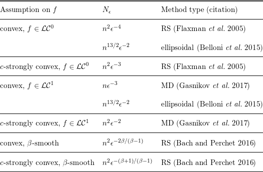
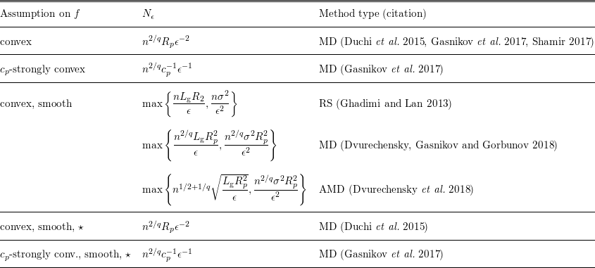
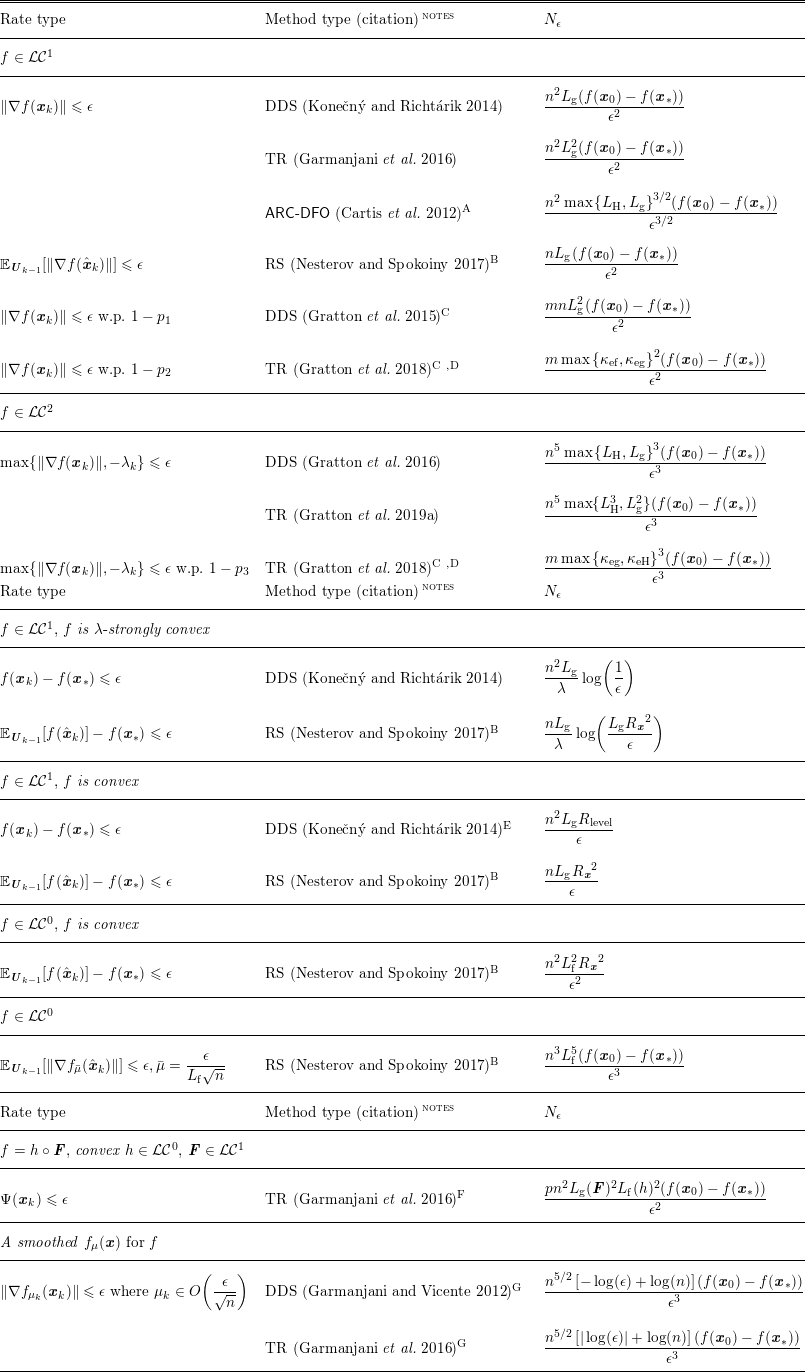
. Throughout this survey, we will refer to Table A.1 for more details concerning specific WCCs. In general, though, we will often summarize WCCs in terms of their
 $\unicode[STIX]{x1D716}$
-dependence, as this provides an asymptotic characterization of a method’s complexity in terms of the accuracy to which one wishes to solve a problem.
When
 $f\in {\mathcal{L}}{\mathcal{C}}^{2}$
, work by Gratton et al. (Reference Gratton, Royer and Vicente2016) essentially augments the DDS method analysed by Vicente (Reference Vicente2013), but forms an approximate Hessian via central differences from function evaluations obtained (for free) by using a particular choice of
 $\boldsymbol{D}_{k}$
. Gratton et al. (Reference Gratton, Royer and Vicente2016) then demonstrate that this augmentation of Algorithm 2has a subsequence that converges to a second-order stationary point. That is, they prove a convergence result of the form (2.7) and demonstrate a WCC result of type (2.3) in
 $O(\unicode[STIX]{x1D716}^{-3})$
(see Table A.1).
We are unaware of WCC results for MADS methods; this situation may be unsurprising since MADS methods are motivated by non-smooth problems, which depend on the generation of a countably infinite number of poll directions. However, WCC results are not necessarily impossible to obtain in structured non-smooth cases, which we discuss in Section 5. We will discuss a special case where smoothing functions of a non-smooth function are assumed to be available in Section 5.3.2.
2.2 Model-based methods
In the context of derivative-free optimization, model-based methods are methods whose updates are based primarily on the predictions of a model that serves as a surrogate of the objective function or of a related merit function. We begin with basic properties and construction of popular models; readers interested in algorithmic frameworks such as trust-region methods and implicit filtering can proceed to Section 2.2.4. Throughout this section, we assume that models are intended as a surrogate for the function
 $f$
; in future sections, these models will be extended to capture functions arising, for example, as constraints or separable components. The methods in this section assume some smoothness in
 $f$
and therefore operate with smooth models; in Section 5, we examine model-based methods that exploit knowledge of non-smoothness.
2.2.1 Quality of smooth model approximation
A natural first indicator of the quality of a model used for optimization is the degree to which the model locally approximates the function
 $f$
and its derivatives. To say anything about the quality of such approximation, one must make an assumption about the smoothness of both the model and function. For the moment, we leave this assumption implicit, but it will be formalized in subsequent sections.
A function
 $m:\mathbb{R}^{n}\rightarrow \mathbb{R}$
is said to be a
 $\boldsymbol{\unicode[STIX]{x1D705}}$
-fully linear model of
 $f$
on
 ${\mathcal{B}}(\boldsymbol{x};\unicode[STIX]{x1D6E5})=\{\boldsymbol{y}~:~\Vert \boldsymbol{x}-\boldsymbol{y}\Vert \leq \unicode[STIX]{x1D6E5}\}$
if
 $$\begin{eqnarray}\displaystyle |f(\boldsymbol{x}+\boldsymbol{s})-m(\boldsymbol{x}+\boldsymbol{s})| & \leq & \displaystyle \unicode[STIX]{x1D705}_{\text{ef}}\unicode[STIX]{x1D6E5}^{2},\quad \text{for all}~\boldsymbol{s}\in {\mathcal{B}}(\mathbf{0};\unicode[STIX]{x1D6E5}),\end{eqnarray}$$
 $$\begin{eqnarray}\displaystyle \Vert \unicode[STIX]{x1D6FB}f(\boldsymbol{x}+\boldsymbol{s})-\unicode[STIX]{x1D6FB}m(\boldsymbol{x}+\boldsymbol{s})\Vert & \leq & \displaystyle \unicode[STIX]{x1D705}_{\text{eg}}\unicode[STIX]{x1D6E5},\quad \text{for all}~\boldsymbol{s}\in {\mathcal{B}}(\mathbf{0};\unicode[STIX]{x1D6E5}),\end{eqnarray}$$
 $\boldsymbol{\unicode[STIX]{x1D705}}=(\unicode[STIX]{x1D705}_{\text{ef}},\unicode[STIX]{x1D705}_{\text{eg}})$
. Similarly, for
 $\boldsymbol{\unicode[STIX]{x1D705}}=(\unicode[STIX]{x1D705}_{\text{ef}},\unicode[STIX]{x1D705}_{\text{eg}},\unicode[STIX]{x1D705}_{\text{eH}})$
,
 $m$
is said to be a
 $\boldsymbol{\unicode[STIX]{x1D705}}$
-fully quadratic model of
 $f$
on
 ${\mathcal{B}}(\boldsymbol{x};\unicode[STIX]{x1D6E5})$
if
 $$\begin{eqnarray}\displaystyle |f(\boldsymbol{x}+\boldsymbol{s})-m(\boldsymbol{x}+\boldsymbol{s})| & \leq & \displaystyle \unicode[STIX]{x1D705}_{\text{ef}}\unicode[STIX]{x1D6E5}^{3},\quad \text{for all}~\boldsymbol{s}\in {\mathcal{B}}(\mathbf{0};\unicode[STIX]{x1D6E5}),\end{eqnarray}$$
 $$\begin{eqnarray}\displaystyle \Vert \unicode[STIX]{x1D6FB}f(\boldsymbol{x}+\boldsymbol{s})-\unicode[STIX]{x1D6FB}m(\boldsymbol{x}+\boldsymbol{s})\Vert & \leq & \displaystyle \unicode[STIX]{x1D705}_{\text{eg}}\unicode[STIX]{x1D6E5}^{2},\quad \text{for all}~\boldsymbol{s}\in {\mathcal{B}}(\mathbf{0};\unicode[STIX]{x1D6E5}),\end{eqnarray}$$
 $$\begin{eqnarray}\displaystyle \Vert \unicode[STIX]{x1D6FB}^{2}f(\boldsymbol{x}+\boldsymbol{s})-\unicode[STIX]{x1D6FB}^{2}m(\boldsymbol{x}+\boldsymbol{s})\Vert & \leq & \displaystyle \unicode[STIX]{x1D705}_{\text{eH}}\unicode[STIX]{x1D6E5},\quad \text{for all}~\boldsymbol{s}\in {\mathcal{B}}(\mathbf{0};\unicode[STIX]{x1D6E5}).\end{eqnarray}$$
Models satisfying (2.9) or (2.10) are called Taylor-like models. To understand why, consider the second-order Taylor model
 $$\begin{eqnarray}m(\boldsymbol{x}+\boldsymbol{s})=f(\boldsymbol{x})+\unicode[STIX]{x1D6FB}f(\boldsymbol{x})^{\text{T}}\boldsymbol{s}+\displaystyle \frac{1}{2}\boldsymbol{s}^{\text{T}}\unicode[STIX]{x1D6FB}^{2}f(\boldsymbol{x})\boldsymbol{s}.\end{eqnarray}$$
This model is a
 $\boldsymbol{\unicode[STIX]{x1D705}}$
-fully quadratic model of
 $f$
, with
 $$\begin{eqnarray}\displaystyle (\unicode[STIX]{x1D705}_{\text{ef}},\unicode[STIX]{x1D705}_{\text{eg}},\unicode[STIX]{x1D705}_{\text{eH}})=(L_{\text{H}}/6,L_{\text{H}}/2,L_{\text{H}}), & & \displaystyle \nonumber\end{eqnarray}$$
on any
 ${\mathcal{B}}(\boldsymbol{x};\unicode[STIX]{x1D6E5})$
, where
 $f$
has a Lipschitz-continuous second derivative with Lipschitz constant
 $L_{\text{H}}$
.
As illustrated in the next section, one also can guarantee that models that do not employ derivative information satisfy these approximation bounds in (2.9) or (2.10). This approximation quality is used by derivative-free algorithms to ensure that a sufficient reduction predicted by the model
 $m$
yields an attainable reduction in the function
 $f$
as
 $\unicode[STIX]{x1D6E5}$
becomes smaller.
2.2.2 Polynomial models
Polynomial models are the most commonly used models for derivative-free local optimization. We let
 ${\mathcal{P}}^{d,n}$
denote the space of polynomials of
 $n$
variables of degree
 $d$
and
 $\boldsymbol{\unicode[STIX]{x1D719}}~:~\mathbb{R}^{n}\rightarrow \mathbb{R}^{\text{dim}({\mathcal{P}}^{d,n})}$
define a basis for this space. For example, quadratic models can be obtained by using the monomial basis
 $$\begin{eqnarray}\boldsymbol{\unicode[STIX]{x1D719}}(\boldsymbol{x})=[1,x_{1},\ldots ,x_{n},x_{1}^{2},\ldots x_{n}^{2},x_{1}x_{2},\ldots ,x_{n-1}x_{n}]^{\text{T}},\end{eqnarray}$$
for which
 $\text{dim}({\mathcal{P}}^{2,n})=(n+1)(n+2)/2$
; linear models can be obtained by using the first
 $\text{dim}({\mathcal{P}}^{1,n})=n+1$
components of (2.12); quadratic models with diagonal Hessians, which are considered by Powell (Reference Powell2003), can be obtained by using the first
 $2n+1$
components of (2.12).
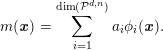
Any polynomial model
 $m\in {\mathcal{P}}^{d,n}$
is defined by
 $\boldsymbol{\unicode[STIX]{x1D719}}$
and coefficients
 $\boldsymbol{a}\in \mathbb{R}^{\text{dim}({\mathcal{P}}^{d,n})}$
through
Given a set of
 $p$
points
 $\boldsymbol{Y}=\{\boldsymbol{y}_{1},\ldots ,\boldsymbol{y}_{p}\}$
, a model that interpolates
 $f$
on
 $\boldsymbol{Y}$
is defined by the solution
 $\boldsymbol{a}$
to
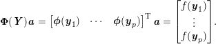 $$\begin{eqnarray}\boldsymbol{\unicode[STIX]{x1D6F7}}(\boldsymbol{Y})\boldsymbol{a}=\left[\begin{array}{@{}ccc@{}}\boldsymbol{\unicode[STIX]{x1D719}}(\boldsymbol{y}_{1}) & \cdots \, & \boldsymbol{\unicode[STIX]{x1D719}}(\boldsymbol{y}_{p})\end{array}\right]^{\text{T}}\boldsymbol{a}=\left[\begin{array}{@{}c@{}}f(\boldsymbol{y}_{1})\\ \vdots \\ f(\boldsymbol{y}_{p})\end{array}\right]\!.\end{eqnarray}$$
The existence, uniqueness and conditioning of a solution to (2.14) depend on the location of the sample points
 $\boldsymbol{Y}$
through the matrix
 $\boldsymbol{\unicode[STIX]{x1D6F7}}(\boldsymbol{Y})$
. We note that when
 $n>1$
,
 $|\boldsymbol{Y}|=\text{dim}({\mathcal{P}}^{d,n})$
is insufficient for guaranteeing that
 $\boldsymbol{\unicode[STIX]{x1D6F7}}(\boldsymbol{Y})$
is non-singular (Wendland Reference Wendland2005). Instead, additional conditions, effectively on the geometry of the sample points
 $\boldsymbol{Y}$
, must be satisfied.
Simplex gradients and linear interpolation models.
The geometry conditions needed to uniquely define a linear model are relatively straightforward: the sample points
 $\boldsymbol{Y}$
must be affinely independent; that is, the columns of
 $$\begin{eqnarray}\boldsymbol{Y}_{-1}=\left[\begin{array}{@{}ccc@{}}\boldsymbol{y}_{2}-\boldsymbol{y}_{1} & \cdots \, & \boldsymbol{y}_{n+1}-\boldsymbol{y}_{1}\end{array}\right]\end{eqnarray}$$
must be linearly independent. Such sample points define what is referred to as a simplex gradient
 $\boldsymbol{g}$
through
 $\boldsymbol{g}=[a_{2},\ldots ,a_{n+1}]^{\text{T}}$
, when the monomial basis
 $\unicode[STIX]{x1D719}$
is used in (2.14).
Simplex gradients can be viewed as a generalization of first-order finite-difference estimates (e.g. the forward differences based on evaluations at the points
 $\{\boldsymbol{y}_{1},\boldsymbol{y}_{1}+\unicode[STIX]{x1D6E5}\boldsymbol{e}_{1},\ldots ,\boldsymbol{y}_{1}+\unicode[STIX]{x1D6E5}\boldsymbol{e}_{n}\}$
); their use in optimization algorithms dates at least back to the work of Spendley et al. (Reference Spendley, Hext and Himsworth1962) that inspired Nelder and Mead (Reference Nelder and Mead1965). Other example usage includes pattern search (Custódio and Vicente Reference Custódio and Vicente2007, Custódio et al.
Reference Custódio, Dennis and Vicente2008) and noisy optimization (Kelley Reference Kelley1999b
, Bortz and Kelley Reference Bortz, Kelley and Borggaard1998); the study of simplex gradients continues with recent works such as those of Regis (Reference Regis2015) and Coope and Tappenden (Reference Coope and Tappenden2019).
Provided that (2.15) is non-singular, it is straightforward to show that linear interpolation models are
 $\boldsymbol{\unicode[STIX]{x1D705}}$
-fully linear model of
 $f$
in a neighbourhood of
 $\boldsymbol{y}_{1}$
. In particular, if
 $\boldsymbol{Y}\subset {\mathcal{B}}(\boldsymbol{y}_{1};\unicode[STIX]{x1D6E5})$
and
 $f$
has an
 $L_{\text{g}}$
-Lipschitz-continuous first derivative on an open domain containing
 ${\mathcal{B}}(\boldsymbol{y}_{1};\unicode[STIX]{x1D6E5})$
, then (2.9) holds on
 ${\mathcal{B}}(\boldsymbol{y}_{1};\unicode[STIX]{x1D6E5})$
with
 $$\begin{eqnarray}\unicode[STIX]{x1D705}_{\text{eg}}=L_{\text{g}}(1+\sqrt{n}\unicode[STIX]{x1D6E5}\Vert \boldsymbol{Y}_{-1}^{-1}\Vert /2)\quad \text{and}\quad \unicode[STIX]{x1D705}_{\text{e f}}=L_{\text{g}}/2+\unicode[STIX]{x1D705}_{\text{eg}}.\end{eqnarray}$$
The expressions in (2.16) also provide a recipe for obtaining a model with a potentially tighter error bound over
 ${\mathcal{B}}(\boldsymbol{y}_{1};\unicode[STIX]{x1D6E5})$
: modify
 $\boldsymbol{Y}\subset {\mathcal{B}}(\boldsymbol{y}_{1};\unicode[STIX]{x1D6E5})$
to decrease
 $\Vert \boldsymbol{Y}_{-1}^{-1}\Vert$
. We note that when
 $\boldsymbol{Y}_{-1}$
contains orthonormal directions scaled by
 $\unicode[STIX]{x1D6E5}$
, one recovers
 $\unicode[STIX]{x1D705}_{\text{eg}}=L_{\text{g}}(1+\sqrt{n}/2)$
and
 $\unicode[STIX]{x1D705}_{\text{ef}}=L_{\text{g}}(3+\sqrt{n})/2$
, which is the least value one can obtain from (2.16) given the restriction that
 $\boldsymbol{Y}\subset {\mathcal{B}}(\boldsymbol{y}_{1};\unicode[STIX]{x1D6E5})$
. Hence, by performing LU or QR factorization with pivoting, one can obtain directions (which are then scaled by
 $\unicode[STIX]{x1D6E5}$
) in order to improve the conditioning of
 $\boldsymbol{Y}_{-1}^{-1}$
and hence the approximation bound. Such an approach is performed by Conn, Scheinberg and Vicente (Reference Conn, Scheinberg and Vicente2008a
) for linear models and by Wild and Shoemaker (Reference Wild and Shoemaker2011) for fully linear radial basis function models.
The geometric conditions on
 $\boldsymbol{Y}$
, induced by the approximation bounds in (2.9) or (2.10), can be viewed as playing a similar role to the geometric conditions (e.g. positive spanning) imposed on
 $\boldsymbol{D}$
in directional direct-search methods. Naturally, the choice of basis function used for any model affects the quantitative measure of that model’s quality.
Note that many practical methods employ interpolation sets contained within a constant multiple of the trust-region radius (i.e.
 $\boldsymbol{Y}\subset {\mathcal{B}}(\boldsymbol{y}_{1};c_{1}\unicode[STIX]{x1D6E5})$
for a constant
 $c_{1}\in [1,\infty )$
).
Quadratic interpolation models.
Quadratic interpolation models have been used for derivative-free optimization for at least fifty years (Winfield Reference Winfield1969, Reference Winfield1973) and were employed by a series of methods that revitalized interest in model-based methods; see, for example, Conn and Toint (Reference Conn, Toint, Di Pillo and Giannessi1996), Conn, Scheinberg and Toint (Reference Conn, Scheinberg and Toint1997b ), Conn, Scheinberg and Toint (Reference Conn, Scheinberg, Toint, Iserles and Buhmann1997a ) and Powell (Reference Powell and Yuan1998b , Reference Powell2002).
Of course, the quality of an interpolation model (quadratic or otherwise) in a region of interest is determined by the position of the underlying points being interpolated. For example, if a model
 $m$
interpolates a function
 $f$
at points far away from a certain region of interest, the model value may differ greatly from the value of
 $f$
in that region.
 $\unicode[STIX]{x1D6EC}$
-poisedness is a concept to measure how well a set of points is dispersed through a region of interest, and ultimately how well a model will estimate the function in that region.
The most commonly used metric for quantifying how well points are positioned in a region of interest is based on Lagrange polynomials. Given a set of
 $p$
points
 $\boldsymbol{Y}=\{\boldsymbol{y}_{1},\ldots ,\boldsymbol{y}_{p}\}$
, a basis of Lagrange polynomials satisfies
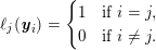 $$\begin{eqnarray}\ell _{j}(\boldsymbol{y}_{i})=\left\{\begin{array}{@{}ll@{}}1\quad & \text{if }i=j,\\ 0\quad & \text{if }i\neq j.\end{array}\right.\end{eqnarray}$$
We now define
 $\unicode[STIX]{x1D6EC}$
-poisedness. A set of points
 $\boldsymbol{Y}$
is said to be
 $\unicode[STIX]{x1D6EC}$
-poised on a set
 $\boldsymbol{B}$
if
 $\boldsymbol{Y}$
is linearly independent and the Lagrange polynomials
 $\{\ell _{1},\ldots ,\ell _{p}\}$
associated with
 $\boldsymbol{Y}$
satisfy
 $$\begin{eqnarray}\unicode[STIX]{x1D6EC}\geq \max _{1\leq i\leq p}\max _{\boldsymbol{x}\in B}|\ell _{i}(\boldsymbol{x})|.\end{eqnarray}$$
(For an equivalent definition of
 $\unicode[STIX]{x1D6EC}$
-poisedness, see Conn et al. (Reference Conn, Scheinberg and Vicente2009b
, Definition 3.6).) Note that the definition of
 $\unicode[STIX]{x1D6EC}$
-poisedness is independent of the function being modelled. Also, the points
 $\boldsymbol{Y}$
need not necessarily be elements of the set
 $\boldsymbol{B}$
. Also, note that if a model is poised on a set
 $\boldsymbol{B}$
, it is poised on any subset of
 $\boldsymbol{B}$
. One is usually interested in the least value of
 $\unicode[STIX]{x1D6EC}$
so that (2.18) holds.
Powell’s unconstrained optimization by quadratic approximation method (UOBYQA) follows such an approach in maximizing the Lagrange polynomials. In Powell (Reference Powell and Yuan1998b ), Powell (Reference Powell2001) and Powell (Reference Powell2002), significant care is given to the linear algebra expense associated with this maximization and the associated change of basis as the methods change their interpolation sets. For example, in Powell (Reference Powell and Yuan1998b ), particular sparsity in the Hessian approximation is employed with the aim of capturing curvature while keeping linear algebraic expenses low.
Maintaining, and the question of to what extent it is necessary to maintain, this geometry for quadratic models has been intensely studied; see, for example, Fasano, Morales and Nocedal (Reference Fasano, Morales and Nocedal2009), Marazzi and Nocedal (Reference Marazzi and Nocedal2002), D’Ambrosio, Nannicini and Sartor (Reference D’Ambrosio, Nannicini and Sartor2017) and Scheinberg and Toint (Reference Scheinberg and Toint2010).
Underdetermined quadratic interpolation models.
A fact not to be overlooked in the context of derivative-free optimization is that employing an interpolation set
 $\boldsymbol{Y}$
requires availability of the
 $|\boldsymbol{Y}|$
function values
 $\{f(\boldsymbol{y}_{i}):\boldsymbol{y}_{i}\in \boldsymbol{Y}\}$
. When the function
 $f$
is computationally expensive to evaluate, the
 $(n+1)(n+2)/2$
points required by fully quadratic models can be a burden, potentially with little benefit, to obtain repeatedly in an optimization algorithm.
Beginning with Powell (Reference Powell2003), Powell investigated quadratic models constructed from fewer than
 $(n+1)(n+2)/2$
points. The most successful of these strategies was detailed in Powell (Reference Powell2004a
) and Powell (Reference Powell2004b
) and resolved the
 $(n+1)(n+2)/2-|\boldsymbol{Y}|$
remaining degrees of freedom by solving problems of the form

to obtain a model
 $m$
about a point of interest
 $\check{\boldsymbol{x}}$
. Solutions to (2.19) are models with a Hessian closest in Frobenius norm to a specified
 $\boldsymbol{H}=\boldsymbol{H}^{\text{T}}$
among all models that interpolate
 $f$
on
 $\boldsymbol{Y}$
. A popular implementation of this strategy is the NEWUOA solver (Powell Reference Powell, Di Pillo and Roma2006).
By using the basis
 $$\begin{eqnarray}\displaystyle \begin{array}{@{}lll@{}}\boldsymbol{\unicode[STIX]{x1D719}}(\check{\boldsymbol{x}}+\boldsymbol{x}) & = & \displaystyle [\boldsymbol{\unicode[STIX]{x1D719}}_{\text{fg}}(\check{\boldsymbol{x}}+\boldsymbol{x})^{\text{T}}|\,\boldsymbol{\unicode[STIX]{x1D719}}_{\text{H}}(\check{\boldsymbol{x}}+\boldsymbol{x})^{\text{T}}]^{\text{T}}\\ & = & \displaystyle \biggl[1,\,x_{1},\,\ldots ,\,x_{n}\bigg|\,\displaystyle \frac{1}{2}x_{1}^{2},\,\ldots ,\,\displaystyle \frac{1}{2}x_{n}^{2},\,\displaystyle \frac{1}{\sqrt{2}}x_{1}x_{2},\,\ldots ,\displaystyle \frac{1}{\sqrt{2}}x_{n-1}x_{n}\biggr]^{\text{T}},\end{array} & & \displaystyle\end{eqnarray}$$
the problem (2.19) is equivalent to the problem

Existence and uniqueness of solutions to (2.21) again depend on the positioning of the points in
 $\boldsymbol{Y}$
. Notably, a necessary condition for there to be a unique minimizer of the seminorm is that at least
 $n+1$
of the points in
 $\boldsymbol{Y}$
be affinely independent. Lagrange polynomials can be defined for this case; Conn, Scheinberg and Vicente (Reference Conn, Scheinberg and Vicente2008b
) establish conditions for
 $\unicode[STIX]{x1D6EC}$
-poisedness (and hence a fully linear, or better, approximation quality) of such models.
Powell (Reference Powell2004c
, Reference Powell2007, Reference Powell2008) develops efficient solution methodologies for (2.21) when
 $\boldsymbol{H}$
and
 $m$
are constructed from interpolation sets that differ by at most one point, and employ these updates in NEWUOA and subsequent solvers. Wild (Reference Wild2008b
) and Custódio et al. (Reference Custódio, Rocha and Vicente2009) use
 $\boldsymbol{H}=\mathbf{0}$
in order to obtain tighter fully linear error bounds of models resulting from (2.21). A strategy of using even fewer interpolation points (including those in a proper subspace of
 $\mathbb{R}^{n}$
) is developed by Powell (Reference Powell2013) and Zhang (Reference Zhang2014). In Section 5.2, we summarize approaches that exploit knowledge of sparsity of the derivatives of
 $f$
in building quadratic models that interpolate fewer than
 $(n+1)(n+2)/2$
points.
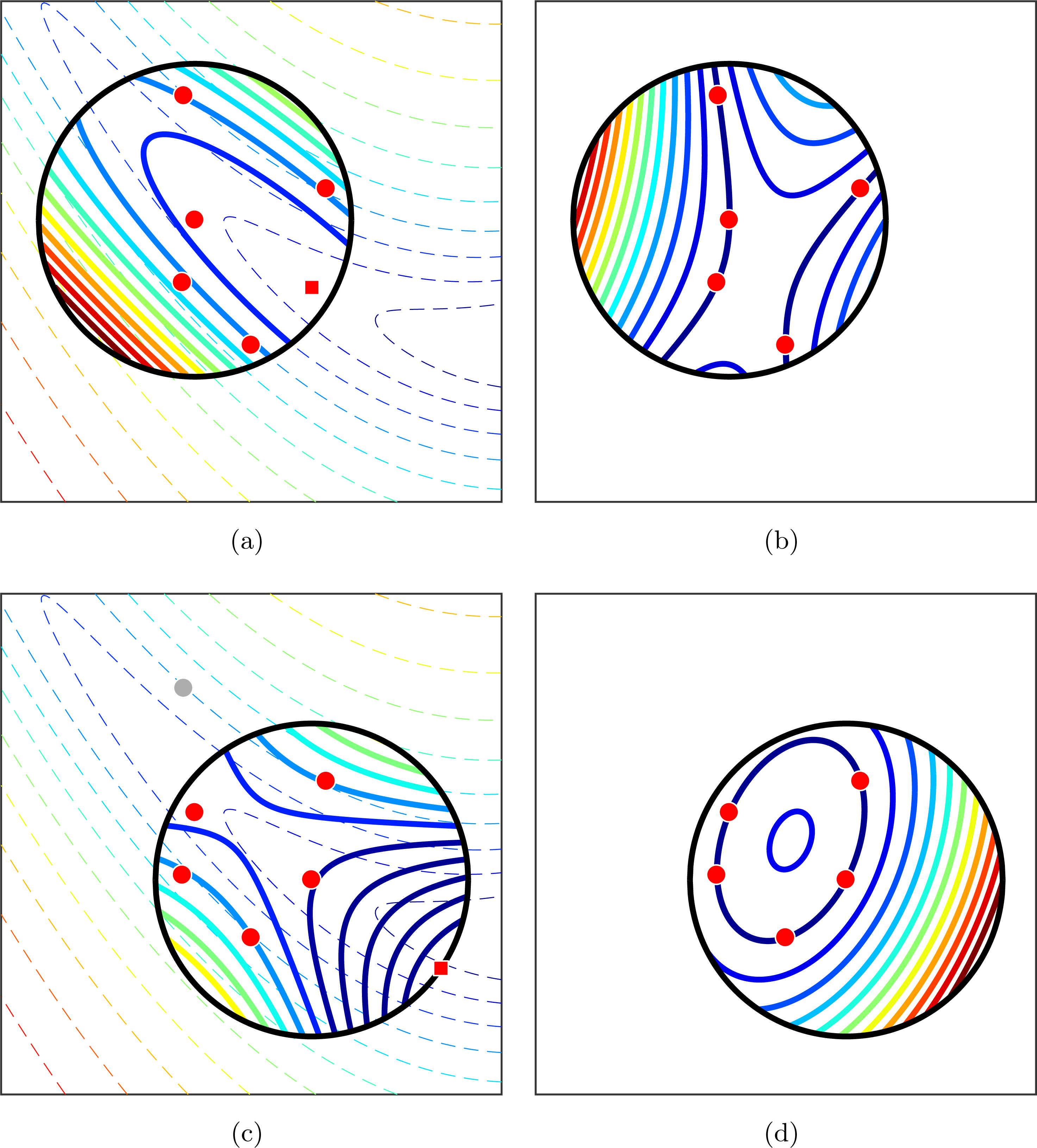
(a) Minimum-norm-Hessian model through five points in
 ${\mathcal{B}}(\boldsymbol{x}_{k};\unicode[STIX]{x1D6E5}_{k})$
and its minimizer. (b) Absolute value of a sixth Lagrange polynomial for the five points. (c) Minimum-norm-Hessian model through five points in
 ${\mathcal{B}}(\boldsymbol{x}_{k+1};\unicode[STIX]{x1D6E5}_{k+1})$
and its minimizer. (d) Absolute value of a sixth Lagrange polynomial for the five points.
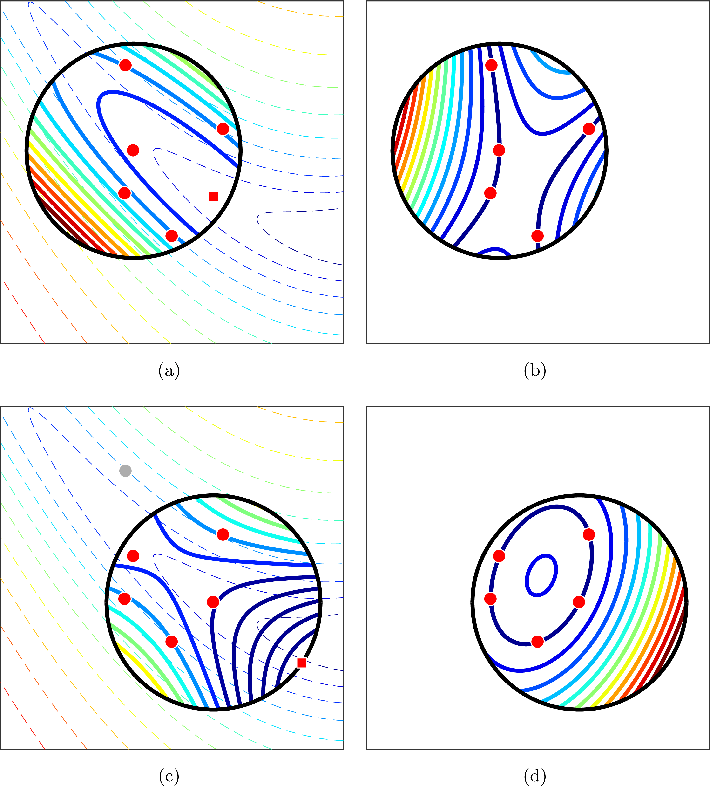
Figure 2.2 shows quadratic models in two dimensions that interpolate
 $(n+1)(n+2)/2-1=5$
points as well as the associated magnitude of the remaining Lagrange polynomial (note that this polynomial vanishes at the five interpolated points).
Regression models.
Just as one can establish approximation bounds and geometry conditions when
 $\boldsymbol{Y}$
is linearly independent, the same can be done for overdetermined regression models (Conn et al.
Reference Conn, Scheinberg and Vicente2008b
, Reference Conn, Scheinberg and Vicente2009b
). This can be accomplished by extending the definition of Lagrange polynomials from (2.17) to the regression case. That is, given a basis
 $\boldsymbol{\unicode[STIX]{x1D719}}~:~\mathbb{R}^{n}\rightarrow \mathbb{R}^{\text{dim}({\mathcal{P}}^{d,n})}$
and points
 $\boldsymbol{Y}=\{\boldsymbol{y}_{1},\ldots ,\boldsymbol{y}_{p}\}\subset \mathbb{R}^{n}$
with
 $p>\text{dim}({\mathcal{P}}^{d,n})$
, the set of polynomials satisfies
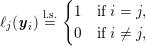 $$\begin{eqnarray}\ell _{j}(\boldsymbol{y}_{i})\overset{\text{l.s.}}{=}\left\{\begin{array}{@{}ll@{}}1\quad & \text{if }i=j,\\ 0\quad & \text{if }i\neq j,\end{array}\right.\end{eqnarray}$$
where
 $\overset{\text{l.s.}}{=}$
denotes the least-squares solution. The regression model can be recovered finding the least-squares solution (now overdetermined) system from (2.14), and the definition of
 $\unicode[STIX]{x1D6EC}$
-poisedness (in the regression sense) is equivalent to (2.18). Ultimately, given a linear regression model through a set of
 $\unicode[STIX]{x1D6EC}$
-poised points
 $\boldsymbol{Y}\subset {\mathcal{B}}(\boldsymbol{y}_{1};\unicode[STIX]{x1D6E5})$
, and if
 $f$
has an
 $L_{\text{g}}$
-Lipschitz-continuous first derivative on an open domain containing
 ${\mathcal{B}}(\boldsymbol{y}_{1};\unicode[STIX]{x1D6E5})$
, then (2.9) holds on
 ${\mathcal{B}}(\boldsymbol{y}_{1};\unicode[STIX]{x1D6E5})$
with
 $$\begin{eqnarray}\unicode[STIX]{x1D705}_{\text{eg}}=\displaystyle \frac{5}{2}\sqrt{p}L_{\text{g}}\unicode[STIX]{x1D6EC}\quad \text{and}\quad \unicode[STIX]{x1D705}_{\text{ef}}=\displaystyle \frac{1}{2}L_{\text{g}}+\unicode[STIX]{x1D705}_{\text{eg}}.\end{eqnarray}$$
Conn et al. (Reference Conn, Scheinberg and Vicente2008b ) note the fact that the extension of Lagrange polynomials does not apply to the 1-norm or infinity-norm case. Billups, Larson and Graf (Reference Billups, Larson and Graf2013) show that the definition of Lagrange polynomials can be extended to the weighted regression case. Verdério, Karas, Pedroso and Scheinberg (Reference Verdério, Karas, Pedroso and Scheinberg2017) show that (2.9) can also be recovered for support vector regression models.
Efficiently minimizing the model (regardless of type) over a trust region is integral to the usefulness of such models within an optimization algorithm. In fact, this necessity is a primary reason for the use of low-degree polynomial models by the majority of derivative-free trust-region methods. For quadratic models, the resulting subproblem remains one of the most difficult non-convex optimization problems solvable in polynomial time, as illustrated by Moré and Sorensen (Reference Moré and Sorensen1983). As exemplified by Powell (Reference Powell and Griffiths1997), the implementation of subproblem solvers is a key concern in methods seeking to perform as few algebraic operations between function evaluations as possible.
2.2.3 Radial basis function interpolation models
An additional way to model non-linearity with potentially less restrictive geometric conditions is by using radial basis functions (RBFs). Such models take the form
 $$\begin{eqnarray}m(\boldsymbol{x})=\mathop{\sum }_{i=1}^{|\boldsymbol{Y}|}b_{i}\unicode[STIX]{x1D713}(\Vert \boldsymbol{x}-\boldsymbol{y}_{i}\Vert )+\boldsymbol{a}^{\text{T}}\boldsymbol{\unicode[STIX]{x1D719}}(\boldsymbol{x}),\end{eqnarray}$$
where
 $\unicode[STIX]{x1D713}~:~\mathbb{R}_{+}\rightarrow \mathbb{R}$
is a conditionally positive-definite univariate function and
 $\boldsymbol{a}^{\text{T}}\boldsymbol{\unicode[STIX]{x1D719}}(\boldsymbol{x})$
represents a (typically low-order) polynomial as before; see, for example, Buhmann (Reference Buhmann2000). Given a sample set
 $\boldsymbol{Y}$
, RBF model coefficients
 $(\boldsymbol{a},\boldsymbol{b})$
can be obtained by solving the augmented interpolation equations
 $$\begin{eqnarray}\left[\begin{array}{@{}cccc@{}}\unicode[STIX]{x1D713}(\Vert \boldsymbol{y}_{1}-\boldsymbol{y}_{1}\Vert ) & \cdots \, & \unicode[STIX]{x1D713}(\Vert \boldsymbol{y}_{1}-\boldsymbol{y}_{|\boldsymbol{Y}|}\Vert ) & \boldsymbol{\unicode[STIX]{x1D719}}(\boldsymbol{y}_{1})^{\text{T}}\\ \vdots & & \vdots & \vdots \\ \unicode[STIX]{x1D713}(\Vert \boldsymbol{y}_{|\boldsymbol{Y}|}-\boldsymbol{y}_{1}\Vert ) & \cdots \, & \unicode[STIX]{x1D713}(\Vert \boldsymbol{y}_{|\boldsymbol{Y}|}-\boldsymbol{y}_{|\boldsymbol{Y}|}\Vert ) & \boldsymbol{\unicode[STIX]{x1D719}}(\boldsymbol{y}_{|\boldsymbol{Y}|})^{\text{T}}\\ \boldsymbol{\unicode[STIX]{x1D719}}(\boldsymbol{y}_{1}) & \cdots \, & \boldsymbol{\unicode[STIX]{x1D719}}(\boldsymbol{y}_{|\boldsymbol{Y}|}) & \mathbf{0}\end{array}\right]\left[\begin{array}{@{}c@{}}\boldsymbol{b}\\ \boldsymbol{a}\end{array}\right]=\left[\begin{array}{@{}c@{}}f(\boldsymbol{y}_{1})\\ \vdots \\ f(\boldsymbol{y}_{|\boldsymbol{Y}|})\\ \mathbf{0}\end{array}\right]\!.\end{eqnarray}$$
That RBFs are conditionally positive-definite ensures that (2.25) is non-singular provided that the degree
 $d$
of the polynomial
 $\boldsymbol{\unicode[STIX]{x1D719}}$
is sufficiently large and that
 $\boldsymbol{Y}$
is poised for degree-
 $d$
polynomial interpolation. For example, cubic (
 $\unicode[STIX]{x1D713}(r)=r^{3}$
) RBFs require a linear polynomial; multiquadric (
 $\unicode[STIX]{x1D713}(r)=-(\unicode[STIX]{x1D6FE}^{2}+r^{2})^{1/2}$
) RBFs require a constant polynomial; and inverse multiquadric (
 $\unicode[STIX]{x1D713}(r)=(\unicode[STIX]{x1D6FE}^{2}+r^{2})^{-1/2}$
) and Gaussian (
 $\unicode[STIX]{x1D713}(r)=\exp (-\unicode[STIX]{x1D6FE}^{-2}r^{2})$
) RBFs do not require a polynomial. Consequently, RBFs have relatively unrestrictive geometric requirements on the interpolation points
 $\boldsymbol{Y}$
while allowing for modelling a wide range of non-linear behaviour.
This feature is typically exploited in global optimization (see e.g. Björkman and Holmström Reference Björkman and Holmström2000, Gutmann Reference Gutmann2001 and Regis and Shoemaker Reference Regis and Shoemaker2007), whereby an RBF surrogate model is employed to globally approximate
 $f$
. However, works such as Oeuvray and Bierlaire (Reference Oeuvray and Bierlaire2009), Oeuvray (Reference Oeuvray2005), Wild (Reference Wild2008a
) and Wild and Shoemaker (Reference Wild and Shoemaker2013) establish and use local approximation properties of these models. This approach is typically performed by relying on a linear polynomial
 $\boldsymbol{a}^{\text{T}}\boldsymbol{\unicode[STIX]{x1D719}}(\boldsymbol{x})$
, which can be used to establish that the RBF model in (2.24) can be a fully linear local approximation of smooth
 $f$
.
2.2.4 Trust-region methods
Having discussed issues of model construction, we are now ready to present a general statement of a model-based trust-region method in Algorithm 3.

A distinguishing characteristic of derivative-free model-based trust-region methods is how they manage
 $\boldsymbol{Y}_{k}$
, the set of points used to construct the model
 $m_{k}$
. Some methods ensure that
 $\boldsymbol{Y}_{k}$
contains a scaled stencil of points around
 $\boldsymbol{x}_{k}$
; such an approach can be attractive since the objective at such points can be evaluated in parallel. A fixed stencil can also ensure that all models sufficiently approximate the objective. Other methods construct
 $\boldsymbol{Y}$
by using previously evaluated points near
 $\boldsymbol{x}_{k}$
, for example, those points within
 ${\mathcal{B}}(\boldsymbol{x}_{k};c_{1}\unicode[STIX]{x1D6E5}_{k})$
for some constant
 $c_{1}\in [1,\infty )$
. Depending on the set of previously evaluated points, such methods may need to add points to
 $\boldsymbol{Y}_{k}$
that most improve the model quality. Determining which additional points to add to
 $\boldsymbol{Y}_{k}$
can be computationally expensive, but the method should be willing to do so in the hope of needing fewer evaluations of the objective function at new points in
 $\boldsymbol{Y}_{k}$
. Most methods do not ensure that models are valid on every iteration but rather make a single step toward improving the model. Such an approach can ensure a high-quality model in a finite number of improvement steps. (Exceptional methods that ensure model quality before
 $\boldsymbol{s}_{k}$
is calculated are the methods of Powell and manifold sampling of Khan, Larson and Wild (Reference Khan, Larson and Wild2018).) The ORBIT method (Wild, Regis and Shoemaker Reference Wild, Regis and Shoemaker2008) places a limit on the size of
 $\boldsymbol{Y}_{k}$
(e.g. in order to limit the amount of linear algebra or to prevent overfitting). In the end, such restrictions on
 $\boldsymbol{Y}_{k}$
may determine whether
 $m_{k}$
is an interpolation or regression model.
Derivative-free trust-region methods share many similarities with traditional trust-region methods, for example, the use of a
 $\unicode[STIX]{x1D70C}$
-test to determine whether a step is taken or rejected. As in a traditional trust-region method, the
 $\unicode[STIX]{x1D70C}$
-test measures the ratio of actual decrease observed in the objective versus the decrease predicted by the model.
On the other hand, the management of the trust-region radius parameter
 $\unicode[STIX]{x1D6E5}_{k}$
in Algorithm 3differs remarkably from traditional trust-region methods. Derivative-free variants require an additional test of model quality, the failure of which results in shrinking
 $\unicode[STIX]{x1D6E5}_{k}$
. When derivatives are available, Taylor’s theorem ensures model accuracy for small
 $\unicode[STIX]{x1D6E5}_{k}$
. In the derivative-free case, such a condition must be explicitly checked in order to ensure that
 $\unicode[STIX]{x1D6E5}_{k}$
does not go to zero merely because the model is poor, hence the inclusion of tests of model quality. As a direct result of these considerations,
 $\unicode[STIX]{x1D6E5}_{k}\rightarrow 0$
as Algorithm 3converges; this is generally not the case in traditional trust-region methods.
As in derivative-based trust-region methods, the solution to the trust-region subproblem in line 11of Algorithm 3must satisfy a Cauchy decrease condition. Given the model
 $m_{k}$
used in Algorithm 3,we define the optimal step length in the direction
 $-\unicode[STIX]{x1D6FB}m_{k}(\boldsymbol{x}_{k})$
by

and the corresponding Cauchy step
 $$\begin{eqnarray}\displaystyle \boldsymbol{s}_{k}^{C}=-t_{k}^{C}\unicode[STIX]{x1D6FB}m_{k}(\boldsymbol{x}_{k}). & & \displaystyle \nonumber\end{eqnarray}$$
It is straightforward to show (see e.g. Conn, Scheinberg and Vicente Reference Conn, Scheinberg and Vicente2009b , Theorem 10.1) that
 $$\begin{eqnarray}m_{k}(\boldsymbol{x}_{k})-m_{k}(\boldsymbol{x}_{k}+\boldsymbol{s}_{k}^{C})\geq \displaystyle \frac{1}{2}\Vert \unicode[STIX]{x1D6FB}m_{k}(\boldsymbol{x}_{k})\Vert \min \left\{\displaystyle \frac{\Vert \unicode[STIX]{x1D6FB}m_{k}(\boldsymbol{x}_{k})\Vert }{\Vert \unicode[STIX]{x1D6FB}^{2}m_{k}(\boldsymbol{x}_{k})\Vert },\unicode[STIX]{x1D6E5}_{k}\right\}.\end{eqnarray}$$
That is, (2.26) states that, provided that both
 $\unicode[STIX]{x1D6E5}_{k}\approx \Vert \unicode[STIX]{x1D6FB}m_{k}(\boldsymbol{x}_{k})\Vert$
and a uniform bound exists on the norm of the model Hessian, the model decrease attained by the Cauchy step
 $\boldsymbol{s}_{k}^{C}$
is of the order of
 $\unicode[STIX]{x1D6E5}_{k}^{2}$
. In order to prove convergence, it is desirable to ensure that each step
 $\boldsymbol{s}_{k}$
generated in line 11of Algorithm 3decreases the model
 $m_{k}$
by no less than
 $\boldsymbol{s}_{k}^{C}$
does, or at least some fixed positive fraction of the decrease achieved by
 $\boldsymbol{s}_{k}^{C}$
. Because successful iterations ensure that the actual decrease attained in an iteration is at least a constant fraction of the model decrease, the sequence of decreases of Algorithm 3are square-summable, provided that
 $\unicode[STIX]{x1D6E5}_{k}\rightarrow 0$
. (This is indeed the case for derivative-free trust-region methods.) Hence, in most theoretical treatments of these methods, it is commonly stated as an assumption that the subproblem solution
 $\boldsymbol{s}_{k}$
obtained in line 11of Algorithm 3satisfies
 $$\begin{eqnarray}m_{k}(\boldsymbol{x}_{k})-m_{k}(\boldsymbol{x}_{k}+\boldsymbol{s}_{k})\geq \unicode[STIX]{x1D705}_{\text{fcd}}(m_{k}(\boldsymbol{x}_{k})-m_{k}(\boldsymbol{x}_{k}+\boldsymbol{s}_{k}^{C})),\end{eqnarray}$$
where
 $\unicode[STIX]{x1D705}_{\text{fcd}}\in (0,1]$
is the fraction of the Cauchy decrease. In practice, when
 $m_{k}$
is a quadratic model, subproblem solvers have been well studied and often come with guarantees concerning the satisfaction of (2.27) (Conn, Gould and Toint Reference Conn, Gould and Toint2000). Wild et al. (Reference Wild, Regis and Shoemaker2008, Figure 4.3) demonstrate the satisfaction of an assumption like (2.27) when the model
 $m_{k}$
is a radial basis function.
Under reasonable smoothness assumptions, most importantly
 $f\in {\mathcal{L}}{\mathcal{C}}^{1}$
, algorithms in the Algorithm 3framework have been shown to be first-order convergent (i.e. (2.4)) and second-order convergent (i.e. (2.6)), with the (arguably) most well-known proof given by Conn, Scheinberg and Vicente (Reference Conn, Scheinberg and Vicente2009a
). In more recent work, Garmanjani, Jùdice and Vicente (Reference Garmanjani, Jùdice and Vicente2016) provide a WCC bound of the form (2.2) for Algorithm 3, recovering essentially the same upper bound on the number of function evaluations required by DDS methods found in Vicente (Reference Vicente2013), that is, a WCC bound in
 $O(\unicode[STIX]{x1D716}^{-2})$
(see Table A.1). When
 $f\in {\mathcal{L}}{\mathcal{C}}^{2}$
, Gratton, Royer and Vicente (Reference Gratton, Royer and Vicente2019a
) demonstrate a second-order WCC bound of the form (2.3) in
 $O(\unicode[STIX]{x1D716}^{-3})$
; in order to achieve this result, fully quadratic models
 $m_{k}$
are required. In Section 3.3, a similar result is achieved by using randomized variants that do not require a fully quadratic model in every iteration.
Early analysis of Powell’s UOBYQA method shows that, with minor modifications, the algorithm can converge superlinearly in neighbourhoods of strict convexity (Han and Liu Reference Han and Liu2004). A key distinction between Powell’s methods and other model-based trust-region methods is the use of separate neighbourhoods for model quality and trust-region steps, with each of these neighbourhoods changing dynamically. Convergence of such methods is addressed by Powell (Reference Powell2010, Reference Powell2012).
The literature on derivative-free trust-region methods is extensive. We mention in passing several additional classes of trust-region methods that have not fallen neatly into our discussion thus far. Wedge methods (Marazzi and Nocedal Reference Marazzi and Nocedal2002) explicitly enforce geometric properties (
 $\unicode[STIX]{x1D6EC}$
-poisedness) of the sample set between iterations by adding additional constraints to the trust-region subproblem. Alexandrov, Dennis, Jr, Lewis and Torczon (Reference Alexandrov, Dennis, Lewis and Torczon1998) consider a trust-region method utilizing a hierarchy of model approximations. In particular, if derivatives can be obtained but are expensive, then the method of Alexandrov et al. (Reference Alexandrov, Dennis, Lewis and Torczon1998) uses a model that interpolates not only zeroth-order information but also first-order (gradient) information. For problems with deterministic noise, Elster and Neumaier (Reference Elster and Neumaier1995) propose a method that projects the solutions of a trust-region subproblem onto a dynamically refined grid, encouraging better practical behaviour. Similarly, for problems with deterministic noise, Maggiar, Wächter, Dolinskaya and Staum (Reference Maggiar, Wächter, Dolinskaya and Staum2018) propose a model-based trust-region method that implicitly convolves the objective function with a Gaussian kernel, again yielding better practical behaviour.
2.3 Hybrid methods and miscellanea
While the majority of work in derivative-free methods for deterministic problems can be classified as direct-search or model-based methods, some work defies this simple classification. In fact, several works (Conn and Le Digabel Reference Conn and Le Digabel2013, Custódio et al. Reference Custódio, Rocha and Vicente2009, Dennis, Jr and Torczon Reference Dennis, Torczon, Alexandrov and Hussaini1997, Frimannslund and Steihaug Reference Frimannslund and Steihaug2011) propose methods that seem to hybridize these two classes, existing somewhere in the intersection. For example, Custódio and Vicente (Reference Custódio and Vicente2005) and Custódio et al. (Reference Custódio, Rocha and Vicente2009) develop the SID-PSM method, which extends Algorithm 2so that the search step consists of minimizing an approximate quadratic model of the objective (obtained either by minimum-Frobenius norm interpolation or by regression) over a trust region. Here, we highlight methods that do not neatly belong to the two aforementioned classes of methods.
2.3.1 Finite differences
As noted in Section 1.1.2, many of the earliest derivative-free methods employed finite-difference-based estimates of derivatives. The most popular first-order directional derivative estimates include the forward/reverse difference
 $$\begin{eqnarray}\unicode[STIX]{x1D6FF}_{\text{f}}(f;\boldsymbol{x};\boldsymbol{d};h)=\displaystyle \frac{f(\boldsymbol{x}+h\boldsymbol{d})-f(\boldsymbol{x})}{h}\end{eqnarray}$$
and central difference
 $$\begin{eqnarray}\unicode[STIX]{x1D6FF}_{\text{c}}(f;\boldsymbol{x};\boldsymbol{d};h)=\displaystyle \frac{f(\boldsymbol{x}+h\boldsymbol{d})-f(\boldsymbol{x}-h\boldsymbol{d})}{2h},\end{eqnarray}$$
where
 $h\neq 0$
is the difference parameter and the non-trivial
 $\boldsymbol{d}\in \mathbb{R}^{n}$
defines the direction. Several recent methods, including the methods described in Sections 2.3.2, 2.3.3 and 3.1.2, use such estimates and employ difference parameters or directions that dynamically change.
As an example of a potentially dynamic choice of difference parameter, we consider the usual case of roundoff errors. We denote by
 $f_{\infty }^{\prime }(\boldsymbol{x};\boldsymbol{d})$
the directional derivative at
 $\boldsymbol{x}$
of the infinite-precision (i.e. based on real arithmetic) objective function
 $f_{\infty }$
in the unit direction
 $\boldsymbol{d}$
(i.e.
 $\Vert \boldsymbol{d}\Vert =1$
). We then have the following error for forward or reverse finite-difference estimates based on the function
 $f$
available through computation:
 $$\begin{eqnarray}|\unicode[STIX]{x1D6FF}_{\text{f}}(f;\boldsymbol{x};\boldsymbol{d};h)-f_{\infty }^{\prime }(\boldsymbol{x};\boldsymbol{d})|\leq \displaystyle \frac{1}{2}L_{\text{g}}(\boldsymbol{x})|h|+2\displaystyle \frac{\unicode[STIX]{x1D716}_{\infty }(\boldsymbol{x})}{|h|},\end{eqnarray}$$
provided that
 $|f_{\infty }^{\prime \prime }(\cdot ;\boldsymbol{d})|\leq L_{\text{g}}(\boldsymbol{x})$
and
 $|f_{\infty }(\cdot )-f(\cdot )|\leq \unicode[STIX]{x1D716}_{\infty }(\boldsymbol{x})$
on the interval
 $[\boldsymbol{x},\boldsymbol{x}+h\boldsymbol{d}]$
. In Gill, Murray and Wright (Reference Gill, Murray and Wright1981) and Gill, Murray, Saunders and Wright (Reference Gill, Murray, Saunders and Wright1983), the recommended difference parameter is
 $h=2\sqrt{\unicode[STIX]{x1D716}_{\infty }(\boldsymbol{x})/L_{\text{g }}(\boldsymbol{x})}$
, which yields the minimum value
 $2\sqrt{\unicode[STIX]{x1D716}_{\infty }(\boldsymbol{x})L_{\text{g }}(\boldsymbol{x})}$
of the upper bound in (2.30); when
 $\unicode[STIX]{x1D716}_{\infty }$
is a bound on the roundoff error and
 $L_{\text{g}}$
is of order one, then the familiar
 $h\in O(\sqrt{\unicode[STIX]{x1D716}_{\infty }})$
is obtained.
Similarly, if one models the error between
 $f_{\infty }$
and
 $f$
as a stationary stochastic process (through the ansatz denoted by
 $f_{\boldsymbol{\unicode[STIX]{x1D709}}}$
) with variance
 $\unicode[STIX]{x1D716}_{\text{f}}(\boldsymbol{x})^{2}$
, minimizing the upper bound on the mean-squared error,
 $$\begin{eqnarray}\mathbb{E}_{\boldsymbol{\unicode[STIX]{x1D709}}}[(\unicode[STIX]{x1D6FF}_{\text{f}}(f_{\boldsymbol{\unicode[STIX]{x1D709}}};\boldsymbol{x};\boldsymbol{d};h)-f_{\infty }^{\prime }(\boldsymbol{x};\boldsymbol{d}))^{2}]\leq \displaystyle \frac{1}{4}L_{\text{g}}(\boldsymbol{x})^{2}h^{2}+2\displaystyle \frac{\unicode[STIX]{x1D716}_{\text{f}}(\boldsymbol{x})^{2}}{h^{2}},\end{eqnarray}$$
yields the choice
 $h=(\sqrt{8}\unicode[STIX]{x1D716}_{\text{f}}(\boldsymbol{x})/L_{\text{g}}(\boldsymbol{x}))^{1/2}$
with an associated root-mean-squared error of
 $(\sqrt{2}\unicode[STIX]{x1D716}_{\infty }(\boldsymbol{x})L_{\text{g}}(\boldsymbol{x}))^{1/2}$
; see, for example, Moré and Wild (Reference Moré and Wild2012, Reference Moré and Wild2014). A rough procedure for computing
 $\unicode[STIX]{x1D716}_{\text{f}}$
is provided in Moré and Wild (Reference Moré and Wild2011) and used in recent methods such as that of Berahas, Byrd and Nocedal (Reference Berahas, Byrd and Nocedal2019).
In both cases (2.30) and (2.31), the first-order error is
 $c\sqrt{\unicode[STIX]{x1D716}(\boldsymbol{x})L_{\text{g }}(\boldsymbol{x})}$
(for a constant
 $c\leq 2$
), which can be used to guide the decision on whether the derivatives estimates are of sufficient accuracy.
2.3.2 Implicit filtering
Implicit filtering is a hybrid of a grid-search algorithm (evaluating all points on a lattice) and a Newton-like local optimization method. The gradient (and possible Hessian) estimates for local optimization are approximated by the central differences
 $\{\unicode[STIX]{x1D6FF}_{\text{c}}(f;\boldsymbol{x}_{k};\boldsymbol{e}_{i};\unicode[STIX]{x1D6E5}_{k}):i=1,\ldots ,n\}$
. The difference parameter
 $\unicode[STIX]{x1D6E5}_{k}$
decreases when implicit filtering encounters a stencil failure at
 $\boldsymbol{x}_{k}$
, that is,
 $$\begin{eqnarray}f(\boldsymbol{x}_{k})\leq f(\boldsymbol{x}_{k}\pm \unicode[STIX]{x1D6E5}_{k}\boldsymbol{e}_{i}),\end{eqnarray}$$
where
 $\boldsymbol{e}_{i}$
is the
 $i$
th elementary basis vector. This is similar to direct-search methods, but notice that implicit filtering is not polling opportunistically: all polling points are evaluated on each iteration.

The basic version of implicit filtering from Kelley (Reference Kelley2011) is outlined in Algorithm 4. Note that most implementations of implicit filtering require a bound-constrained domain.
Considerable effort has been devoted to extensions of Algorithm 4when
 $f$
is ‘noisy’. Gilmore and Kelley (Reference Gilmore and Kelley1995) show that implicit filtering converges to local minima of (DET) when the objective
 $f$
is the sum of a smooth function
 $f_{s}$
and a high-frequency, low-amplitude function
 $f_{n}$
, with
 $f_{n}\rightarrow 0$
quickly in a neighbourhood of all minimizers of
 $f_{s}$
. Under similar assumptions, Choi and Kelley (Reference Choi and Kelley2000) show that Algorithm 4converges superlinearly if the step sizes
 $\unicode[STIX]{x1D6E5}_{k}$
are defined as a power of the norm of the previous iteration’s gradient approximation.
2.3.3 Adaptive regularized methods
Cartis, Gould and Toint (Reference Cartis, Gould and Toint2012) perform an analysis of adaptive regularized cubic (ARC) methods and propose a derivative-free method, ARC-DFO. ARC-DFO is an extension of ARC whereby gradients are replaced with central finite differences of the form (2.29), with the difference parameter monotonically decreasing within a single iteration of the method. ARC-DFO is an intrinsically model-based method akin to Algorithm 3, but the objective within each subproblem regularizes third-order behaviour of the model. Thus, like a trust-region method, ARC-DFO employs trial steps and model gradients. During the main loop of ARC-DFO, if the difference parameter exceeds a constant factor of the minimum of the trial step norm or the model gradient norm, then the difference parameter is shrunk by a constant factor, and the iteration restarts to obtain a new trial step. This mechanism is structurally similar to a derivative-free trust-region method’s checks on model quality. Cartis et al. (Reference Cartis, Gould and Toint2012) show that ARC-DFO demonstrates a WCC result of type (2.2) in
 $O(\unicode[STIX]{x1D716}^{-3/2})$
, the same asymptotic result (in terms of
 $\unicode[STIX]{x1D716}$
-dependence) that the authors demonstrate for derivative-based variants of ARC methods. In terms of dependence on
 $\unicode[STIX]{x1D716}$
, this result is a strict improvement over the WCC results of the same type demonstrated for DDS and trust-region methods, although this result is proved under the stronger assumption that
 $f\in {\mathcal{L}}{\mathcal{C}}^{2}$
.
In a different approach, Hare and Lucet (Reference Hare and Lucet2013) show convergence of a derivative-free method that penalizes large steps via a proximal regularizer, thereby removing the necessity for a trust region. Lazar and Jarre (Reference Lazar and Jarre2016) regularize their line-search with a term seeking to minimize a weighted change of the model’s third derivatives.
2.3.4 Line-search-based methods
Several line-search-based methods for derivative-free optimization have been developed. Grippo, Lampariello and Lucidi (Reference Grippo, Lampariello and Lucidi1988) and De Leone, Gaudioso and Grippo (Reference De Leone, Gaudioso and Grippo1984) (two of the few papers appearing in the 1980s concerning derivative-free optimization) both analyse conditions on the step sizes used in a derivative-free line-search algorithm, and provide methods for constructing such steps. Lucidi and Sciandrone (Reference Lucidi and Sciandrone2002b
) present methods that combine pattern-search and line-search approaches in a convergent framework. The VXQR method of Neumaier, Fendl, Schilly and Leitner (Reference Neumaier, Fendl, Schilly and Leitner2011) performs a line search on a direction computed from a QR factorization of previously evaluated points. Neumaier et al. (Reference Neumaier, Fendl, Schilly and Leitner2011) apply VXQR to problems with
 $n=1000$
, a large problem dimension among the methods considered here.
Consideration has also been given to non-monotone line-search-based derivative-free methods. Since gradients are not available in derivative-free optimization, the search direction in a line-search method may not be a descent direction. Non-monotone methods allow one to still employ such directions in a globally convergent framework. Grippo and Sciandrone (Reference Grippo and Sciandrone2007) extend line-search strategies based on coordinate search and the method of Barzilai and Borwein (Reference Barzilai and Borwein1988) to develop a globally convergent non-monotone derivative-free method. Grippo and Rinaldi (Reference Grippo and Rinaldi2014) extend such non-monotone strategies to broader classes of algorithms that employ simplex gradients, hence further unifying direct-search and model-based methods. Another non-monotone line-search method is proposed by Diniz-Ehrhardt, Martínez and Raydan (Reference Diniz-Ehrhardt, Martínez and Raydan2008), who encapsulate early examples of randomized DDS methods (Section 3.2).
2.3.5 Methods for non-smooth optimization
In Section 2.1.2, we discuss how MADS handles non-differentiable objective functions by densely sampling directions on a mesh, thereby ensuring that all Clarke directional derivatives are non-negative (i.e. (2.1)). Another early analysis of a DDS method on a class of non-smooth objectives was performed by García-Palomares and Rodríguez (Reference García-Palomares and Rodríguez2002).
Gradient sampling methods are a developing class of algorithms for general non-smooth non-convex optimization; see the recent survey by Burke et al. (Reference Burke, Curtis, Lewis, Overton and Simões2018). These methods attempt to estimate the
 $\unicode[STIX]{x1D716}$
-subdifferential at a point
 $\boldsymbol{x}$
by evaluating a random sample of gradients in the neighbourhood of
 $\boldsymbol{x}$
and constructing the convex hull of these gradients. In a derivative-free setting, the approximation of these gradients is not as immediately obvious in the presence of non-smoothness, but there exist gradient-sampling methods that use finite-difference estimates with specific smoothing techniques (Kiwiel Reference Kiwiel2010).
In another distinct line of research, Bagirov, Karasözen and Sezer (Reference Bagirov, Karasözen and Sezer2007) analyse a derivative-free variant of subgradient descent, where subgradients are approximated via so-called discrete gradients. In Section 5.3, we will further discuss methods for minimizing composite non-smooth objective functions of the form
 $f=h\circ F$
, where
 $h$
is non-smooth but a closed-form expression is known and
 $F$
is assumed smooth. These methods are characterized by their exploitation of the knowledge of
 $h$
, making them less general than the methods for non-smooth optimization discussed so far.
3 Randomized methods for deterministic objectives
We now summarize randomized methods for solving (DET). Such methods often have promising theoretical properties, although some practitioners may dislike the non-deterministic behaviour of these methods. We discuss randomization within direct-search methods in Section 3.2 and within trust-region methods in Section 3.3, but we first begin with a discussion of random search as applied to deterministic objectives.
In any theoretical treatment of randomized methods, one must be careful to distinguish between random variables and their realizations. For the sake of terseness in this survey, we will intentionally conflate variables with realizations and refer to respective papers for more careful statements of theoretical results.
3.1 Random search
We highlight two randomized methods for minimizing a deterministic objective: pure random search and Nesterov random search.
3.1.1 Pure random search
Pure random search is a natural method to start with for randomized derivative-free optimization. Pure random search is popular for multiple reasons; in particular, it is easy to implement (with few or no user-defined tolerances), and (if the points generated are independent of one another) it exhibits perfect scaling in terms of evaluating
 $f$
at many points simultaneously.
A pure random-search method is given in Algorithm 5, where points are generated randomly from
 $\boldsymbol{\unicode[STIX]{x1D6FA}}$
. For example, if
 $\boldsymbol{\unicode[STIX]{x1D6FA}}=\{\boldsymbol{x}:\boldsymbol{c}(\boldsymbol{x})\leq \mathbf{0},\boldsymbol{l}\leq \boldsymbol{x}\leq \boldsymbol{u}\}$
, line 3of Algorithm 5may involve drawing points uniformly at random from
 $[\boldsymbol{l},\boldsymbol{u}]$
and checking whether they satisfy
 $\boldsymbol{c}(\boldsymbol{x})\leq \mathbf{0}$
.

If the procedure for generating points in line 3of Algorithm 5is independent of the function values observed, then the entire set of points used within pure random search can be generated beforehand: we intentionally omit the index
 $k$
in the statement of Algorithm 5.
Nevertheless, for the sake of analysis, it is useful to consider an ordering of the sequence of random points generated by Algorithm 5.With such a sequence
 $\{\boldsymbol{x}_{k}\}$
, one can analyse the best points after
 $N$
evaluations,

If
 $f_{\ast }$
is the global minimum value, then
 $$\begin{eqnarray}\displaystyle \mathbb{P}[f(\hat{\boldsymbol{x}}_{N})\leq f_{\ast }+\unicode[STIX]{x1D716}]=1-\mathop{\prod }_{k=1}^{N}(1-\mathbb{P}[\boldsymbol{x}_{k}\in \boldsymbol{{\mathcal{L}}}_{f_{\ast }+\unicode[STIX]{x1D716}}(f)]), & & \displaystyle \nonumber\end{eqnarray}$$
where
 $\unicode[STIX]{x1D716}\geq 0$
and
 $\boldsymbol{{\mathcal{L}}}_{\unicode[STIX]{x1D6FC}}(f)=\{\boldsymbol{x}:f(\boldsymbol{x})\leq \unicode[STIX]{x1D6FC}\}$
. Provided that the procedure used to generate points at line 3of Algorithm 5satisfies
 $$\begin{eqnarray}\displaystyle \lim _{N\rightarrow \infty }\mathop{\prod }_{k=1}^{N}(1-\mathbb{P}[\boldsymbol{x}_{k}\in \boldsymbol{{\mathcal{L}}}_{f_{\ast }+\unicode[STIX]{x1D716}}(f)])=0 & & \displaystyle \nonumber\end{eqnarray}$$
for all
 $\unicode[STIX]{x1D716}>0$
, then
 $f(\hat{\boldsymbol{x}}_{k})$
converges in probability to
 $f_{\ast }$
. For example, if each
 $\boldsymbol{x}_{k}$
is drawn independently and uniformly over
 $\boldsymbol{\unicode[STIX]{x1D6FA}}$
, then one can calculate the number of evaluations required to ensure that the
 $\hat{\boldsymbol{x}}_{k}$
returned by Algorithm 5satisfies
 $\hat{\boldsymbol{x}}_{k}\in \boldsymbol{{\mathcal{L}}}_{f_{\ast }+\unicode[STIX]{x1D716}}$
with probability
 $p\in (0,1)$
, that is,
 $$\begin{eqnarray}\displaystyle N\geq \displaystyle \frac{\log (p)}{\log \biggl(1-\displaystyle \frac{\unicode[STIX]{x1D707}(\boldsymbol{{\mathcal{L}}}_{f_{\ast }+\unicode[STIX]{x1D716}}\bigcap \boldsymbol{\unicode[STIX]{x1D6FA}})}{\unicode[STIX]{x1D707}(\boldsymbol{\unicode[STIX]{x1D6FA}})}\biggr)}, & & \displaystyle \nonumber\end{eqnarray}$$
provided
 $\unicode[STIX]{x1D707}(\boldsymbol{{\mathcal{L}}}_{f(\boldsymbol{x}_{\ast })+\unicode[STIX]{x1D716}}\cap \boldsymbol{\unicode[STIX]{x1D6FA}})>0$
and
 $\boldsymbol{\unicode[STIX]{x1D6FA}}$
is measurable.
Random-search methods typically make few assumptions about
 $f$
; see Zhigljavsky (Reference Zhigljavsky1991) for further discussion about the convergence of pure random search. Naturally, a method that assumes only that
 $f$
is measurable on
 $\boldsymbol{\unicode[STIX]{x1D6FA}}$
is likely to produce function values that converge more slowly to
 $f_{\ast }$
when applied to an
 $f\in {\mathcal{C}}^{0}$
than does a method that exploits the continuity of
 $f$
. Heuristic modifications of random search have sought to improve empirical performance on certain classes of problems, while still maintaining random search’s global optimization property; see, for example, the work of Zabinsky and Smith (Reference Zabinsky and Smith1992) and Patel, Smith and Zabinsky (Reference Patel, Smith and Zabinsky1989).
3.1.2 Nesterov random search
We refer to the method discussed in this section as Nesterov random search because of the seminal article by Nesterov and Spokoiny (Reference Nesterov and Spokoiny2017), but the idea driving this method is much older. A similar method, for instance, is discussed in Polyak (Reference Polyak1987, Chapter 3.4).
The method of Nesterov random search is largely motivated by Gaussian smoothing. In particular, given a covariance (i.e. symmetric positive-definite) matrix
 $\boldsymbol{B}$
and a smoothing parameter
 $\unicode[STIX]{x1D707}>0$
, consider the Gaussian smoothed function
 $$\begin{eqnarray}\displaystyle f_{\unicode[STIX]{x1D707}}(\boldsymbol{x})=\sqrt{\displaystyle \frac{\text{det}(\boldsymbol{B})}{(2\unicode[STIX]{x1D70B})^{n}}}\int _{\mathbb{R}^{n}}f(\boldsymbol{x}+\unicode[STIX]{x1D707}\boldsymbol{u})\exp \biggl(-\displaystyle \frac{1}{2}\boldsymbol{u}^{\text{T}}\boldsymbol{B}\boldsymbol{u}\biggr)\text{d}\boldsymbol{u}. & & \displaystyle \nonumber\end{eqnarray}$$
This smoothing has many desirable properties; for instance, if
 $f$
is Lipschitz-continuous with constant
 $L_{\text{f}}$
, then
 $f_{\unicode[STIX]{x1D707}}$
is Lipschitz-continuous with a constant no worse than
 $L_{\text{f}}$
for all
 $\unicode[STIX]{x1D707}>0$
. Likewise, if
 $f$
has Lipschitz-continuous gradients with constant
 $L_{\text{g}}$
, then
 $f_{\unicode[STIX]{x1D707}}$
has Lipschitz-continuous gradients with a constant no worse than
 $L_{\text{g}}$
for all
 $\unicode[STIX]{x1D707}>0$
. If
 $f$
is convex, then
 $f_{\unicode[STIX]{x1D707}}$
is convex.
One can show that
 $$\begin{eqnarray}\displaystyle \unicode[STIX]{x1D6FB}f_{\unicode[STIX]{x1D707}}(\boldsymbol{x})=\displaystyle \frac{1}{\unicode[STIX]{x1D707}}\sqrt{\displaystyle \frac{\text{det}(\boldsymbol{B})}{(2\unicode[STIX]{x1D70B})^{n}}}\int _{\mathbb{R}^{n}}(f(\boldsymbol{x}+\unicode[STIX]{x1D707}\boldsymbol{u})-f(\boldsymbol{x}))\exp \biggl(-\displaystyle \frac{1}{2}\boldsymbol{u}^{\text{T}}\boldsymbol{B}\boldsymbol{u}\biggr)\boldsymbol{B}\boldsymbol{u}\text{d}\boldsymbol{u}. & & \displaystyle \nonumber\end{eqnarray}$$
In other words,
 $\unicode[STIX]{x1D6FB}f_{\unicode[STIX]{x1D707}}(\boldsymbol{x})$
, which can be understood as an approximation of
 $\unicode[STIX]{x1D6FB}f(\boldsymbol{x})$
in the smooth case, can be computed via an expectation over
 $\boldsymbol{u}\in \mathbb{R}^{n}$
weighted by the finite difference
 $f(\boldsymbol{x}+\unicode[STIX]{x1D707}\boldsymbol{u})-f(\boldsymbol{x})$
and inversely weighted by a radial distance from
 $\boldsymbol{x}$
. With this interpretation in mind, Nesterov and Spokoiny (Reference Nesterov and Spokoiny2017) propose a collection of random gradient-free oracles, where one first generates a Gaussian random vector
 $\boldsymbol{u}\in {\mathcal{N}}(\mathbf{0},\boldsymbol{B}^{-1})$
and then uses one of
 $$\begin{eqnarray}\begin{array}{@{}lll@{}}\boldsymbol{g}_{\unicode[STIX]{x1D707}}(\boldsymbol{x};\boldsymbol{u}) & = & \unicode[STIX]{x1D6FF}_{\text{f}}(f;\boldsymbol{x};\boldsymbol{u};\unicode[STIX]{x1D707})\boldsymbol{B}\boldsymbol{u},\quad \text{or}\\ \hat{\boldsymbol{g}}_{\unicode[STIX]{x1D707}}(\boldsymbol{x};\boldsymbol{u}) & = & \unicode[STIX]{x1D6FF}_{\text{c}}(f;\boldsymbol{x};\boldsymbol{u};\unicode[STIX]{x1D707})\boldsymbol{B}\boldsymbol{u},\end{array}\end{eqnarray}$$
for a difference parameter
 $\unicode[STIX]{x1D707}>0$
. Nesterov and Spokoiny also propose a third oracle,
 $\boldsymbol{g}_{0}(\boldsymbol{x};\boldsymbol{u})=f^{\prime }(\boldsymbol{x};\boldsymbol{u})\boldsymbol{B}\boldsymbol{u}$
, intended for the optimization of non-smooth functions; this oracle assumes the ability to compute directional derivatives
 $f^{\prime }(\boldsymbol{x};\boldsymbol{u})$
. For this reason, Nesterov and Spokoiny refer to all oracles as gradient-free instead of derivative-free. Given the scope of this survey, we focus on the derivative-free oracles
 $\boldsymbol{g}_{\unicode[STIX]{x1D707}}$
and
 $\hat{\boldsymbol{g}}_{\unicode[STIX]{x1D707}}$
displayed in (3.1).
With an oracle
 $\boldsymbol{g}$
chosen as either oracle in (3.1), Nesterov random-search methods are straightforward to define, and we do so in Algorithm 6. In Algorithm 6,
 $\text{proj}(\cdot ;\boldsymbol{\unicode[STIX]{x1D6FA}})$
denotes projection onto a domain
 $\boldsymbol{\unicode[STIX]{x1D6FA}}$
.

A particularly striking result proved in Nesterov and Spokoiny (Reference Nesterov and Spokoiny2017) was perhaps the first WCC result for an algorithm (Algorithm 6) in the case where
 $f\in {\mathcal{L}}{\mathcal{C}}^{0}$
– that is,
 $f$
may be both non-smooth and non-convex. Because of the randomized nature of iteratively sampling from a Gaussian distribution in Algorithm 6, complexity results are given as expectations. That is, letting
 $\boldsymbol{U}_{k}=\{\boldsymbol{u}_{0},\boldsymbol{u}_{1},\ldots ,\boldsymbol{u}_{k}\}$
denote the random variables associated with the first
 $k$
iterations of Algorithm 6, complexity results are stated in terms of expectations with respect to the filtration defined by these variables. A WCC is given as an upper bound on the number of
 $f$
evaluations needed to attain the approximate (
 $\unicode[STIX]{x1D716}>0$
) optimality condition
 $$\begin{eqnarray}\mathbb{E}_{\boldsymbol{U}_{k-1}}[\Vert \unicode[STIX]{x1D6FB}f_{\check{\unicode[STIX]{x1D707}}}(\hat{\boldsymbol{x}}_{k})\Vert ]\leq \unicode[STIX]{x1D716},\end{eqnarray}$$
where
 $\hat{\boldsymbol{x}}_{k}=\text{arg}\,\text{min}_{j=0,1,\ldots ,k-1}f(\boldsymbol{x}_{j})$
. By fixing a particular choice of
 $\check{\unicode[STIX]{x1D707}}$
(dependent on
 $\unicode[STIX]{x1D716}$
,
 $n$
and Lipschitz constants), Nesterov and Spokoiny (Reference Nesterov and Spokoiny2017) demonstrate that the number of
 $f$
evaluations needed to attain (3.2) is in
 $O(\unicode[STIX]{x1D716}^{-3})$
; see Table A.1. For
 $f\in {\mathcal{L}}{\mathcal{C}}^{1}$
(but still non-convex), Nesterov and Spokoiny (Reference Nesterov and Spokoiny2017) prove a WCC result of type (3.2) in
 $O(\unicode[STIX]{x1D716}^{-2})$
for the same method. WCC results of Algorithm 6under a variety of stronger assumptions on the convexity and differentiability of
 $f$
are also shown in Table A.1 and discussed in Section 4. We further note that some randomized methods of the form Algorithm 6have also been developed for (STOCH), which we discuss in Section 6.
We remark on an undesirable feature of the convergence analysis for variants of Algorithm 6: the analysis of these methods supposes that the sequence
 $\{\unicode[STIX]{x1D6FC}_{k}\}$
is chosen as a constant that depends on parameters, including
 $L_{\text{f}}$
, that may not be available to the method. Similar assumptions concerning the preselection of
 $\{\unicode[STIX]{x1D6FC}_{k}\}$
also appear in the convex cases discussed in Section 4, and we highlight these dependencies in Table A.1.
3.2 Randomized direct-search methods
Randomization has also been used in the DDS framework discussed in Section 2.1 in the hope of more efficiently using evaluations of
 $f$
. Polling every point in a PSS requires at least
 $n+1$
function evaluations; if
 $f$
is expensive to evaluate and
 $n$
is relatively large, this can be wasteful. A deterministic strategy for performing fewer evaluations on many iterations is opportunistic polling. Work in randomized direct-search methods attempts to address, formalize and analyse the situation where polling directions are randomly sampled from some distribution in each iteration. The ultimate goal is to replace the
 $O(n)$
per-iteration function evaluation cost with an
 $O(1)$
per-iteration cost,Footnote
4
while still guaranteeing some form of global convergence.
In Section 2.1, we mentioned MADS methods that consider the random generation of polling directions in each iteration (in order to satisfy the asymptotic density required of search directions for the minimization of non-smooth, but Lipschitz-continuous,
 $f$
). Examples include Audet and Dennis, Jr (Reference Audet and Dennis2006) and Van Dyke and Asaki (Reference Van Dyke and Asaki2013), which implement LTMADS and QRMADS, respectively. While this direction of research is within the scope of randomized methods, the purpose of randomization in MADS methods is to overcome particular difficulties encountered when optimizing general non-smooth objectives. This particular randomization does not fall within the scope of this section, where randomization is intended to decrease a method’s dependence on
 $n$
. In the remainder of this section, we focus on a body of work that seems to exist entirely for the unconstrained case where
 $f$
is assumed sufficiently smooth.
Gratton, Royer, Vicente and Zhang (Reference Gratton, Royer, Vicente and Zhang2015) extend the direct-search framework (Algorithm 2) by assuming that the set of polling directions
 $\boldsymbol{D}_{k}$
includes only a descent direction with probability
 $p$
(as opposed to assuming
 $\boldsymbol{D}_{k}$
always includes a descent direction, which comes for free when
 $f\in {\mathcal{L}}{\mathcal{C}}^{1}$
provided
 $\boldsymbol{D}_{k}$
is, for example, a PSS). To formalize, given
 $p\in (0,1)$
, a random sequence of polling directions
 $\{\boldsymbol{D}_{k}\}$
is said to be
 $p$
-probabilistically
 $\unicode[STIX]{x1D705}_{\text{d}}$
-descent provided that, given a deterministic starting point
 $\boldsymbol{x}_{0}$
,
 $$\begin{eqnarray}\mathbb{P}[\text{cm}([\boldsymbol{D}_{0},-\unicode[STIX]{x1D6FB}f(\boldsymbol{x}_{0})])\geq \unicode[STIX]{x1D705}_{\text{d}}]\geq p,\end{eqnarray}$$
and for all
 $k\geq 1$
,
 $$\begin{eqnarray}\mathbb{P}[\text{cm}([\boldsymbol{D}_{k},-\unicode[STIX]{x1D6FB}f(\boldsymbol{x}_{k})])\geq \unicode[STIX]{x1D705}_{\text{d}}\mid \boldsymbol{D}_{0},\ldots ,\boldsymbol{D}_{k-1}]\geq p,\end{eqnarray}$$
where
 $\text{cm}(\cdot )$
is the cosine measure in (2.8). A collection of polling directions
 $\boldsymbol{D}_{k}$
satisfying (3.3) and (3.4) can be obtained by drawing directions uniformly on the unit ball.
As with the other methods in this section,
 $\boldsymbol{x}_{k}$
in (3.4) is in fact a random variable due to the random sequence
 $\{\boldsymbol{D}_{k}\}$
generated by the algorithm, and hence it makes sense to view (3.4) as a probabilistic statement. In words, (3.4) states that with probability at least
 $p$
, the set of polling directions used in iteration
 $k$
has a positive cosine measure with the steepest descent direction
 $-\unicode[STIX]{x1D6FB}f(\boldsymbol{x}_{k})$
, regardless of the past history of the algorithm. Gratton et al. (Reference Gratton, Royer, Vicente and Zhang2015) use Chernoff bounds in order to bound the worst-case complexity with high probability. Roughly, they show that if
 $f\in {\mathcal{L}}{\mathcal{C}}^{1}$
, and if (3.3) and (3.4) hold with
 $p>1/2$
(this constant changing when
 $\unicode[STIX]{x1D6FE}_{\text{dec}}\neq 1/\unicode[STIX]{x1D6FE}_{\text{inc}}$
), then
 $\Vert \unicode[STIX]{x1D6FB}f(\boldsymbol{x}_{k})\Vert \leq \unicode[STIX]{x1D716}$
holds within
 $O(\unicode[STIX]{x1D716}^{-2})$
function evaluations with a probability that increases exponentially to 1 as
 $\unicode[STIX]{x1D716}\rightarrow 0$
. The WCC result of Gratton et al. (Reference Gratton, Royer, Vicente and Zhang2015) demonstrates that as
 $p\rightarrow 1$
(i.e.
 $\boldsymbol{D}_{k}$
almost always includes a descent direction), the known WCC results for Algorithm 2discussed in Section 2.1.2 are recovered. A more precise statement of this WCC result is included in Table A.1.
Bibi et al. (Reference Bibi, Bergou, Sener, Ghanem and Richtárik2019) propose a randomized direct-search method in which the two poll directions in each iteration are
 $\boldsymbol{D}_{k}=\{\boldsymbol{e}_{i},-\boldsymbol{e}_{i}\}$
, where
 $\boldsymbol{e}_{i}$
is the
 $i$
th elementary basis vector. In the
 $k$
th iteration,
 $\boldsymbol{e}_{i}$
is selected from
 $\{\boldsymbol{e}_{1},\ldots ,\boldsymbol{e}_{n}\}$
with a probability proportional to the Lipschitz constant of the
 $i$
th partial derivative of
 $f$
. Bibi et al. (Reference Bibi, Bergou, Sener, Ghanem and Richtárik2019) perform WCC analysis of this method assuming a known upper bound on Lipschitz constants of partial derivatives; this assumption leads to improved constant factors, but they essentially prove an upper bound on the number of iterations needed to attain
 $\mathbb{E}[\Vert \unicode[STIX]{x1D6FB}f(\boldsymbol{x}_{k})\Vert ]\leq \unicode[STIX]{x1D716}$
in
 $O(\unicode[STIX]{x1D716}^{-2})$
, where the expectation is with respect to the random sequence of
 $\boldsymbol{D}_{k}$
. Bibi et al. (Reference Bibi, Bergou, Sener, Ghanem and Richtárik2019) prove additional WCC results in cases where
 $f$
is convex or
 $c$
-strongly convex.
An early randomized DDS derivative-free method that only occasionally employs a descent direction is developed by Diniz-Ehrhardt et al. (Reference Diniz-Ehrhardt, Martínez and Raydan2008). There, a non-monotone line-search strategy is used to accommodate search directions along which descent may not be initially apparent. Belitz and Bewley (Reference Belitz and Bewley2013) develop a randomized DDS method that employs surrogates and an adaptive lattice.
3.3 Randomized trust-region methods
Whereas the theoretical convergence of a DDS method depends on the set of polling directions satisfying some spanning property (e.g. a cosine measure bounded away from zero), the theoretical convergence of a trust-region method (e.g. Algorithm 3) depends on the use of fully linear models. Analogous to how randomized DDS methods relax the requirement of the use of a positive spanning set in every iteration, (3.4), it is reasonable to ask whether one can relax the requirement of being fully linear in every iteration of a trust-region method. Practically speaking, in the unconstrained case it may not be necessary to ensure that every model is built by using a
 $\unicode[STIX]{x1D6EC}$
-poised set of points (therefore ensuring that the model is fully linear) on every iteration, since ensuring
 $\unicode[STIX]{x1D6EC}$
-poised sets entails additional function evaluations.
Bandeira, Scheinberg and Vicente (Reference Bandeira, Scheinberg and Vicente2014) consider a sequence of random models
 $\{m_{k}\}$
and a random sequence of trust-region centres and radii
 $\{\boldsymbol{x}_{k},\unicode[STIX]{x1D6E5}_{k}\}$
. They say that the sequence of random models is
 $p$
-probabilistically
 $\boldsymbol{\unicode[STIX]{x1D705}}$
-fully linear provided
 $$\begin{eqnarray}\mathbb{P}[m_{k}\text{ is a }\boldsymbol{\unicode[STIX]{x1D705}}\text{-fully linear model of }f\text{ on }{\mathcal{B}}(\boldsymbol{x}_{k};\unicode[STIX]{x1D6E5}_{k})\mid {\mathcal{H}}_{k-1}]\geq p,\end{eqnarray}$$
where
 ${\mathcal{H}}_{k-1}$
is the filtration of the random process prior to the current iteration. That is,
 ${\mathcal{H}}_{k-1}$
is the
 $\unicode[STIX]{x1D70E}$
-algebra generated by the algorithm’s history. Under additional standard assumptions concerning Algorithm 3(e.g.
 $\unicode[STIX]{x1D6FE}_{\text{dec}}=1/\unicode[STIX]{x1D6FE}_{\text{inc}}$
), the authors show that if (3.5) holds with
 $p>1/2$
, then
 $\lim _{k\rightarrow \infty }\Vert \unicode[STIX]{x1D6FB}f(\boldsymbol{x}_{k})\Vert =0$
almost surely (i.e. with probability one). Gratton, Royer, Vicente and Zhang (Reference Gratton, Royer, Vicente and Zhang2018) build on this result; they demonstrate that, up to constants, the same (with high probability) WCC bound that was proved for DDS methods in Gratton et al. (Reference Gratton, Royer, Vicente and Zhang2015) holds for the randomized trust-region method proposed by Bandeira et al. (Reference Bandeira, Scheinberg and Vicente2014). Higher-order versions of (3.5) also exist; in Section 5.2 we discuss settings for which Bandeira et al. (Reference Bandeira, Scheinberg and Vicente2014) obtain probabilistically
 $\boldsymbol{\unicode[STIX]{x1D705}}$
-fully quadratic models by interpolating
 $f$
on a set of fewer than
 $(n+1)(n+2)/2$
points.
4 Methods for convex objectives
As is true of derivative-based optimization, convexity in the objective of (DET) or (STOCH) can be exploited either when designing new methods or when analysing existing methods. Currently, this split falls neatly into two categories. The majority of work considering (DET) when
 $f$
is convex sharpens the WCCs for frameworks already discussed in this survey. On the other hand, the influence of machine learning, particularly large-scale empirical risk minimization, has led to entirely new derivative-free methods for solving (STOCH) when
 $f$
is convex.
4.1 Methods for deterministic convex optimization
We first turn our attention to the solution of (DET). In convex optimization, one can prove WCC bounds on the difference between a method’s estimate of the global minimum of
 $f$
and the value of
 $f$
at a global minimizer
 $\boldsymbol{x}_{\ast }\in \boldsymbol{\unicode[STIX]{x1D6FA}}$
(i.e. a point satisfying
 $f(\boldsymbol{x}_{\ast })\leq f(\boldsymbol{x})$
for all
 $\boldsymbol{x}\in \boldsymbol{\unicode[STIX]{x1D6FA}}$
). This differs from the local WCC bounds on the objective gradient, namely (2.4), that are commonly shown when
 $f$
is not assumed to be convex. For convex
 $f$
, under appropriate additional assumptions, one typically demonstrates that a method satisfies
 $$\begin{eqnarray}\lim _{k\rightarrow \infty }f(\boldsymbol{x}_{k})-f(\boldsymbol{x}_{\ast })=0,\end{eqnarray}$$
where
 $\boldsymbol{x}_{k}$
is the
 $k$
th point of the method. Hence, an appropriate measure of
 $\unicode[STIX]{x1D716}$
-optimality when minimizing an unconstrained convex objective is the satisfaction of
 $$\begin{eqnarray}f(\boldsymbol{x}_{k})-f(\boldsymbol{x}_{\ast })\leq \unicode[STIX]{x1D716}.\end{eqnarray}$$
For the DDS methods discussed in Section 2.1.2, Dodangeh and Vicente (Reference Dodangeh and Vicente2016) and Dodangeh, Vicente and Zhang (Reference Dodangeh, Vicente and Zhang2016) analyse the worst-case complexity of Algorithm 2when there is no search step and when
 $f$
is smooth and convex, and has a bounded level set. By imposing an appropriate upper bound on the step sizes
 $\unicode[STIX]{x1D6FC}_{k}$
, and (for
 $c>0$
) using a test of the form
 $$\begin{eqnarray}f(\boldsymbol{p}_{i})\leq f(\boldsymbol{x}_{k})-c\unicode[STIX]{x1D6FC}_{k}^{2},\end{eqnarray}$$
in line 4of Algorithm 2, Dodangeh and Vicente (Reference Dodangeh and Vicente2016) show that the worst-case number of
 $f$
evaluations to achieve (2.2) is in
 $O(n^{2}L_{\text{g}}^{2}\unicode[STIX]{x1D716}^{-1})$
. Dodangeh et al. (Reference Dodangeh, Vicente and Zhang2016) show that this
 $n^{2}$
-dependence is optimal (in the sense that it cannot be improved) within the class of deterministic methods that employ positive spanning sets. Recall from Section 3.2 that randomized methods allow one to reduce this dependence to be linear in
 $n$
. Under additional assumptions, which are satisfied, for example, when
 $f$
is strongly convex, Dodangeh and Vicente (Reference Dodangeh and Vicente2016) prove
 $R$
-linear convergence of Algorithm 2, yielding a WCC of type (4.2) with the dependence on
 $\unicode[STIX]{x1D716}$
reduced to
 $\log (\unicode[STIX]{x1D716}^{-1})$
. We note that, in the convex setting,
 $R$
-linear convergence had been previously established for a DDS method by Dolan et al. (Reference Dolan, Lewis and Torczon2003). It is notable that the method analysed in Dolan et al. (Reference Dolan, Lewis and Torczon2003) requires only strict decrease, whereas, to the authors’ knowledge, the DDS methods for which WCC results have been established all require sufficient decrease.
Konečný and Richtárik (Reference Konečný and Richtárik2014) propose a DDS method that does not allow for increases in the step size
 $\unicode[STIX]{x1D6FC}_{k}$
and analyse the method on strongly convex, convex and non-convex objectives. Although Konečný and Richtárik (Reference Konečný and Richtárik2014) demonstrate WCC bounds with the same dependence on
 $n$
and
 $\unicode[STIX]{x1D716}$
as do Dodangeh and Vicente (Reference Dodangeh and Vicente2016), they additionally assume that one has explicit knowledge of a Lipschitz gradient constant
 $L_{\text{g}}$
and can thus replace the test (4.3) explicitly with
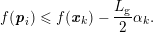 $$\begin{eqnarray}f(\boldsymbol{p}_{i})\leq f(\boldsymbol{x}_{k})-\displaystyle \frac{L_{\text{g}}}{2}\unicode[STIX]{x1D6FC}_{k}.\end{eqnarray}$$
Exploiting this additional knowledge of
 $L_{\text{g}}$
, the WCC result in Konečný and Richtárik (Reference Konečný and Richtárik2014) exhibits a strictly better dependence on
 $L_{\text{g}}$
than does the WCC result in Dodangeh and Vicente (Reference Dodangeh and Vicente2016), with a WCC of type (4.2) in
 $O(n^{2}L_{\text{g}}\unicode[STIX]{x1D716}^{-1})$
. Additionally assuming
 $f$
is
 $c$
-strongly convex, Konečný and Richtárik (Reference Konečný and Richtárik2014) provide a result showing a WCC of type (4.2) in
 $O(\log (\unicode[STIX]{x1D716}^{-1}))$
.
In the non-convex case, Konečný and Richtárik (Reference Konečný and Richtárik2014) recover the same WCC of type (2.2) from Vicente (Reference Vicente2013); see the discussion in Section 2.1. Once again, however, the result by Konečný and Richtárik (Reference Konečný and Richtárik2014) assumes knowledge of
 $L_{\text{g}}$
and again recovers a strictly better dependence on
 $L_{\text{g}}$
by using the test (4.4) in line 4of Algorithm 2.
Recalling the Nesterov random search methods discussed in Section 3.1.2, we remark that Nesterov and Spokoiny (Reference Nesterov and Spokoiny2017) explicitly give results for deterministic, convex
 $f$
. In particular, Nesterov and Spokoiny prove WCCs of a specific type. Because of the randomized nature of Algorithm 6, WCCs are given as expectations of the form
 $$\begin{eqnarray}\mathbb{E}_{\boldsymbol{U}_{k-1}}[f(\hat{\boldsymbol{x}}_{k})]-f(\boldsymbol{x}_{\ast })\leq \unicode[STIX]{x1D716},\end{eqnarray}$$
where
 $\hat{\boldsymbol{x}}_{k}=\text{arg}\,\text{min}_{j\in \{0,1,\ldots ,k-1\}}f(\boldsymbol{x}_{j})$
and where
 $\boldsymbol{U}_{k-1}=\{\boldsymbol{u}_{0},\boldsymbol{u}_{1},\ldots ,\boldsymbol{u}_{k-1}\}$
is the filtration of Gaussian samples. The form of
 $\unicode[STIX]{x1D716}$
-optimality represented by (4.5) can be interpreted as a probabilistic variant of (4.2). The WCC results of Nesterov and Spokoiny show that the worst-case number of
 $f$
evaluations to achieve (4.5) is in
 $O(\unicode[STIX]{x1D716}^{-1})$
when
 $f\in {\mathcal{L}}{\mathcal{C}}^{1}$
. Additionally assuming that
 $f$
is
 $c$
-strongly convex yields an improved result; the WCC of type (4.5) is now in
 $O(\log (\unicode[STIX]{x1D716}^{-1}))$
. Moreover, by mimicking the method of accelerated gradient descent (see e.g. Nesterov Reference Nesterov2004, Chapter 2.2), Nesterov and Spokoiny present a variant of Algorithm 6with a WCC of type (4.5) in
 $O(\unicode[STIX]{x1D716}^{-1/2})$
. When
 $f\in {\mathcal{L}}{\mathcal{C}}^{0}$
, Nesterov and Spokoiny provide a WCC of type (4.5) in
 $O(\unicode[STIX]{x1D716}^{-2})$
, but this result assumes that Algorithm 6uses an oracle with access to exact directional derivatives of
 $f$
. Thus, the method achieves the
 $O(\unicode[STIX]{x1D716}^{-2})$
result when
 $f\in {\mathcal{L}}{\mathcal{C}}^{0}$
is not a derivative-free method.
As remarked in Section 3, these convergence results depend on preselecting a sequence of step sizes
 $\{\unicode[STIX]{x1D6FC}_{k}\}$
for Algorithm 6; in the convex case, the necessary
 $\{\unicode[STIX]{x1D6FC}_{k}\}$
depends not only on the Lipschitz constants but also on a bound
 $R_{\boldsymbol{x}}$
on the distance between the initial point and the global minimizer (i.e.
 $\Vert \boldsymbol{x}_{0}-\boldsymbol{x}_{\ast }\Vert \leq R_{\boldsymbol{x}}$
). The aforementioned WCC results will hold only if one chooses
 $\{\unicode[STIX]{x1D6FC}_{k}\}$
and
 $\unicode[STIX]{x1D707}$
(the difference parameter of the oracle used in Algorithm 6) that scale with
 $L_{\text{g}}$
and
 $R_{\boldsymbol{x}}$
appropriately. When additionally assuming
 $f$
is
 $c$
-strongly convex,
 $\{\unicode[STIX]{x1D6FC}_{k}\}$
and
 $\unicode[STIX]{x1D707}$
also depend on
 $c$
. Stich, Müller and Gärtner (Reference Stich, Müller and Gärtner2013)Footnote
5
extend the framework of Algorithm 6with an approximate line search that avoids the need for predetermined sequences of step sizes.
In general, the existing WCC results for derivative-free methods match the WCC results for their derivative-based counterparts in
 $\unicode[STIX]{x1D716}$
-dependence. The WCC results for derivative-free methods tend to involve an additional factor of
 $n$
when compared with their derivative-based counterparts. This observation mirrors a common intuition in derivative-free optimization: since a number of
 $f$
evaluations in
 $O(n)$
can guarantee a suitable approximation of the gradient, then for any class of gradient-based method for which we replace gradients with approximate gradients or model gradients, one should expect to recover the WCC of that method, but with an extra factor of
 $n$
. WCC results such as those discussed thus far in this survey add credence to this intuition. As we will see in Section 4.2, however, this optimistic trend does not always hold: we will see problem classes for which derivative-free methods are provably worse than their derivative-based counterparts by a factor of
 $\unicode[STIX]{x1D716}^{-1}$
.
Bauschke, Hare and Moursi (Reference Bauschke, Hare and Moursi2014) offer an alternative approach to Algorithm 6for the solution of (DET) when
 $f$
is assumed convex and, additionally, lower-
 ${\mathcal{C}}^{2}$
. (Such an assumption on
 $f$
is obviously stronger than plain convexity but contains, for example, functions that are defined as the pointwise maximum over a collection of convex functions.) Bauschke et al. (Reference Bauschke, Hare and Moursi2014) show that linear interpolation through function values is sufficient for obtaining approximate subgradients of convex, lower-
 ${\mathcal{C}}^{2}$
function; these approximate subgradients are used in lieu of subgradients in a mirror-descent algorithm (see e.g. Srebro, Sridharan and Tewari Reference Srebro, Sridharan, Tewari and Shawe-Taylor2011) similar to Algorithm 7in Section 4.2.2. Bauschke et al. (Reference Bauschke, Hare and Moursi2014) establish convergence of their method in the sense of (4.1), and they demonstrate the performance of their method when applied to pointwise maxima of collections of convex quadratics.
4.2 Methods for convex stochastic optimization
We now turn our attention to the solution of the problem (STOCH) when
 $\tilde{f}(\boldsymbol{x};\boldsymbol{\unicode[STIX]{x1D709}})$
is assumed convex in
 $\boldsymbol{x}$
for each realization
 $\boldsymbol{\unicode[STIX]{x1D709}}$
. Up to this point in the survey, we have typically assumed that (STOCH) is unconstrained, that is,
 $\boldsymbol{\unicode[STIX]{x1D6FA}}=\mathbb{R}^{n}$
. In this section, however, it will become more frequent that
 $\boldsymbol{\unicode[STIX]{x1D6FA}}$
is a compact set.
In the machine learning community, zeroth-order information (i.e. evaluations of
 $\tilde{f}$
only) is frequently referred to as bandit feedback,Footnote
6
due to the concept of multi-armed bandits from reinforcement learning. Multi-armed bandit problems are sequential allocation problems defined by a prescribed set of actions. Robbins (Reference Robbins1952) formulates a multi-armed bandit problem as a gambler’s desire to minimize the total losses accumulated from pulling discrete sequence (of length
 $T$
) of
 $A<\infty$
slot machine arms. The gambler does not have to decide the full length-
 $T$
sequence up front. Rather, at time
 $k\leq T$
, the losses associated with the first
 $k-1$
pulls are known to the gambler when deciding which of the
 $A$
arms to pull next. The gambler’s decision of the
 $k$
th arm to pull is represented by the scalar variable
 $x_{k}\in \boldsymbol{\unicode[STIX]{x1D6FA}}$
. Given additional environmental variables outside the gambler’s control,
 $\boldsymbol{\unicode[STIX]{x1D709}}_{k}\in \boldsymbol{\unicode[STIX]{x1D6EF}}$
, which represents the stochastic nature of the slot machine,Footnote
7
the environment makes a decision
 $\boldsymbol{\unicode[STIX]{x1D709}}$
simultaneously with the gambler’s decision
 $x$
. The gambler’s loss is then
 $\tilde{f}(x;\boldsymbol{\unicode[STIX]{x1D709}})$
.
Within this multi-armed bandit setting, the typical metric of the gambler’s performance is the cumulative regret. Provided that the expectation
 $\mathbb{E}_{\boldsymbol{\unicode[STIX]{x1D709}}}[\tilde{f}(x;\boldsymbol{\unicode[STIX]{x1D709}})]=f(x)$
exists for each
 $x\in \{1,\ldots ,A\}$
, then the gambler’s best long-run strategy in terms of minimizing the expected total losses is to constantly play
 $x_{\ast }\in \text{arg}\,\text{min}_{x\in \{1,\ldots ,A\}}f(x)$
. If, over the course of
 $T$
pulls, the gambler makes a sequence of decisions
 $x_{1},\ldots ,x_{T}$
and the environment makes a sequence of decisions
 $\boldsymbol{\unicode[STIX]{x1D709}}_{1},\ldots ,\boldsymbol{\unicode[STIX]{x1D709}}_{T}$
resulting in a sequence of realized losses
 $\tilde{f}(x_{1};\boldsymbol{\unicode[STIX]{x1D709}}_{1}),\ldots ,\tilde{f}(x_{T};\boldsymbol{\unicode[STIX]{x1D709}}_{T})$
, then the cumulative regret
 $r_{T}$
associated with the gambler’s sequence of decisions is the difference between the cumulative loss incurred by the gambler’s strategy
 $(x_{1},\ldots ,x_{T})$
and the loss incurred by the best possible long-run strategy
 $(x_{\ast },\ldots ,x_{\ast })$
. Analysis of methods for bandit problems in this set-up is generally concerned with expected cumulative regret
 $$\begin{eqnarray}\mathbb{E}_{\boldsymbol{\unicode[STIX]{x1D709}}}[r_{T}(x_{1},\ldots ,x_{T})]=\mathbb{E}_{\boldsymbol{\unicode[STIX]{x1D709}}}\biggl[\mathop{\sum }_{k=1}^{T}\tilde{f}(x_{k};\boldsymbol{\unicode[STIX]{x1D709}}_{k})\biggr]-Tf(x_{\ast }),\end{eqnarray}$$
where the expectation is computed over
 $\boldsymbol{\unicode[STIX]{x1D709}}\in \boldsymbol{\unicode[STIX]{x1D6EF}}$
, since we assume here that the sequence of
 $\boldsymbol{\unicode[STIX]{x1D709}}_{k}$
is independent and identically distributed.
This particular treatment of the bandit problem with a discrete space of actions
 $x\in \{1,\ldots ,A\}$
was the one considered by Robbins (Reference Robbins1952) and has been given extensive treatment (Auer, Cesa-Bianchi, Freund and Schapire Reference Auer, Cesa-Bianchi, Freund and Schapire2003, Lai and Robbins Reference Lai and Robbins1985, Agrawal Reference Agrawal1995, Auer, Cesa-Bianchi and Fischer Reference Auer, Cesa-Bianchi and Fischer2002).
Extending multi-armed bandit methods to infinite-armed bandits makes the connections to derivative-free optimization – particularly derivative-free convex optimization – readily apparent. Auer (Reference Auer2002) extends the multi-armed bandit problem to allow for a compact (as opposed to discrete) set of actions for the gambler
 $\boldsymbol{x}\in \boldsymbol{\unicode[STIX]{x1D6FA}}\subset \mathbb{R}^{n}$
as well as a compact set of vectors for the environment,
 $\boldsymbol{\unicode[STIX]{x1D709}}\in \boldsymbol{\unicode[STIX]{x1D6EF}}\subset \mathbb{R}^{n}$
. The vectors
 $\boldsymbol{\unicode[STIX]{x1D709}}$
in this set-up define linear functions; that is, if the gambler chooses
 $\boldsymbol{x}_{k}$
in their
 $k$
th pull, and the environment chooses
 $\boldsymbol{\unicode[STIX]{x1D709}}_{k}\in \boldsymbol{\unicode[STIX]{x1D6EF}}$
, then the gambler incurs loss
 $\tilde{f}(\boldsymbol{x}_{k};\boldsymbol{\unicode[STIX]{x1D709}}_{k})=\boldsymbol{\unicode[STIX]{x1D709}}_{k}^{\text{T}}\boldsymbol{x}_{k}$
. In this linear regime, expected regret takes a form remarkably similar to (4.6), that is,
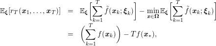 $$\begin{eqnarray}\displaystyle \begin{array}{@{}rcl@{}}\mathbb{E}_{\boldsymbol{\unicode[STIX]{x1D709}}}[r_{T}(\boldsymbol{x}_{1},\ldots ,\boldsymbol{x}_{T})] & = & \displaystyle \mathbb{E}_{\boldsymbol{\unicode[STIX]{x1D709}}}\biggl[\mathop{\sum }_{k=1}^{T}\tilde{f}(\boldsymbol{x}_{k};\boldsymbol{\unicode[STIX]{x1D709}}_{k})\biggr]-\min _{\boldsymbol{x}\in \boldsymbol{\unicode[STIX]{x1D6FA}}}\mathbb{E}_{\boldsymbol{\unicode[STIX]{x1D709}}}\biggl[\mathop{\sum }_{k=1}^{T}\tilde{f}(\boldsymbol{x}_{k};\boldsymbol{\unicode[STIX]{x1D709}}_{k})\biggr]\\ & = & \displaystyle \biggl(\mathop{\sum }_{k=1}^{T}f(\boldsymbol{x}_{k})\biggr)-Tf(\boldsymbol{x}_{\ast }),\end{array} & & \displaystyle\end{eqnarray}$$
with
 $\boldsymbol{x}_{\ast }\in \text{arg}\,\text{min}_{\boldsymbol{x}\in \boldsymbol{\unicode[STIX]{x1D6FA}}}f(\boldsymbol{x})$
. As in (4.6), (4.7) defines the expected regret with respect to the best long-run strategy
 $\boldsymbol{x}\in \boldsymbol{\unicode[STIX]{x1D6FA}}$
that the gambler could have played for the
 $T$
rounds (i.e. the strategy that would minimize the expected cumulative losses).Footnote
8
By using a bandit method known as Thompson sampling, one can show (under appropriate additional assumptions) that if
 $\tilde{f}(\boldsymbol{x};\boldsymbol{\unicode[STIX]{x1D709}})=\boldsymbol{\unicode[STIX]{x1D709}}^{\text{T}}\boldsymbol{x}$
, then (4.7) can be bounded as
 $$\begin{eqnarray}\displaystyle \mathbb{E}_{\boldsymbol{\unicode[STIX]{x1D709}}}[r_{T}(\boldsymbol{x}_{1},\ldots ,\boldsymbol{x}_{T})]\in O(n\sqrt{T\log (T)}) & & \displaystyle \nonumber\end{eqnarray}$$
(Russo and Van Roy Reference Russo and Van Roy2016). Analysis of bounds on (4.7) in the linear case raises an interesting question: to what extent can similar analysis be performed for classes of functions
 $\tilde{f}(\boldsymbol{x};\boldsymbol{\unicode[STIX]{x1D709}})$
that are non-linear in
 $\boldsymbol{x}$
?
In much of the bandit literature, the additional structure defining a class of non-linear functions is convexity; here, by convexity, we mean that
 $\tilde{f}(\boldsymbol{x};\boldsymbol{\unicode[STIX]{x1D709}})$
is convex in
 $\boldsymbol{x}$
for each realization
 $\boldsymbol{\unicode[STIX]{x1D709}}\in \boldsymbol{\unicode[STIX]{x1D6EF}}$
.
Regret bounds on (4.7) automatically imply WCC results for stochastic convex optimization. To see this, define an average point
 $$\begin{eqnarray}\displaystyle \bar{\boldsymbol{x}}_{k}=\displaystyle \frac{1}{k}\mathop{\sum }_{t=1}^{k}\boldsymbol{x}_{t}. & & \displaystyle \nonumber\end{eqnarray}$$
Because of the convexity of
 $f$
,
 $$\begin{eqnarray}f(\bar{\boldsymbol{x}}_{T})-f(\boldsymbol{x}_{\ast })\leq \displaystyle \frac{1}{T}\mathop{\sum }_{k=1}^{T}f(\boldsymbol{x}_{k})-f(\boldsymbol{x}_{\ast })=\displaystyle \frac{\mathbb{E}_{\boldsymbol{\unicode[STIX]{x1D709}}}[r_{T}(\boldsymbol{x}_{1},\ldots ,\boldsymbol{x}_{T})]}{T},\end{eqnarray}$$
where the inequality follows from an application of Jensen’s inequality. We see in (4.8) that, given an upper bound of
 $\bar{r}(T)$
on the expected regret
 $\mathbb{E}_{\boldsymbol{\unicode[STIX]{x1D709}}}[r_{T}]$
, we can automatically derive, provided
 $\bar{r}(T)/T\leq \unicode[STIX]{x1D716}$
, a WCC result for stochastic convex optimization of the form
 $$\begin{eqnarray}\mathbb{E}_{\boldsymbol{\unicode[STIX]{x1D709}}}[\tilde{f}(\bar{\boldsymbol{x}}_{T};\boldsymbol{\unicode[STIX]{x1D709}})-\tilde{f}(\boldsymbol{x}_{\ast };\boldsymbol{\unicode[STIX]{x1D709}})]=f(\bar{\boldsymbol{x}}_{T})-f(\boldsymbol{x}_{\ast })\leq \unicode[STIX]{x1D716}.\end{eqnarray}$$
Equation (4.9) corresponds to a stochastic version of a WCC result of type (4.2) where
 $N_{\unicode[STIX]{x1D716}}=T$
.
The converse implication, however, is not generally true: a small optimization error does not imply a small regret. That is, WCC results of type (4.9) do not generally imply bounds on expected regret (4.7). This is particularly highlighted by Shamir (Reference Shamir, Shalev-Shwartz and Steinwart2013), who considers a class of strongly convex quadratic objectives
 $f$
. For such objectives, Shamir (Reference Shamir, Shalev-Shwartz and Steinwart2013) establishes a strict gap between the upper bound on the optimization error (the left-hand side of (4.9)) and the lower bound on the expected regret (4.7) attainable by any method in the bandit setting. Such a gap, between expected regret and optimization error, has also been proved for bandit methods applied to problems of logistic regression (Hazan, Koren and Levy Reference Hazan, Koren, Levy and Balcan2014).
Results such as those of Shamir (Reference Shamir, Shalev-Shwartz and Steinwart2013), Jamieson, Nowak and Recht (Reference Jamieson, Nowak, Recht and Pereira2012) and Hazan et al. (Reference Hazan, Koren, Levy and Balcan2014) have led researchers to consider methods of derivative-free (stochastic) optimization within the paradigm of convex bandit learning. In this survey, we group these methods into two categories of assumptions on the type of bandit feedback (i.e. the observed realizations of
 $\tilde{f}$
) available to the method: one-point bandit feedback or two-point (multi-point) bandit feedback. Although many of the works we cite have also analysed regret bounds for these methods, we focus on optimization error.
4.2.1 One-point bandit feedback
In one-point bandit feedback, a method is assumed to have access to an oracle
 $\tilde{f}$
that returns unbiased estimates of
 $f$
. In particular, given two points
 $\boldsymbol{x}_{1}$
,
 $\boldsymbol{x}_{2}\in \boldsymbol{\unicode[STIX]{x1D6FA}}$
, two separate calls to the oracle will return
 $\tilde{f}(\boldsymbol{x}_{1};\boldsymbol{\unicode[STIX]{x1D709}}_{1})$
and
 $\tilde{f}(\boldsymbol{x}_{2};\boldsymbol{\unicode[STIX]{x1D709}}_{2})$
; methods do not have control over the selection of the random variables
 $\boldsymbol{\unicode[STIX]{x1D709}}_{1}$
and
 $\boldsymbol{\unicode[STIX]{x1D709}}_{2}$
. Many one-point bandit methods do not fall neatly into the frameworks discussed in this survey (Agarwal et al.
Reference Agarwal, Foster, Hsu, Kakade, Rakhlin and Shawe-Taylor2011, Belloni, Liang, Narayanan and Rakhlin Reference Belloni, Liang, Narayanan and Rakhlin2015, Bubeck, Lee and Eldan Reference Bubeck, Lee and Eldan2017). See Table 4.1 for a summary of best known WCC results of type (4.9) for one-point bandit feedback methods.
One example of a method using one-point bandit feedback, whose development falls naturally into our discussion thus far, is given by Flaxman, Kalai and McMahan (Reference Flaxman, Kalai and McMahan2005); they analyse a method resembling Algorithm 6, but the gradient-free oracle is chosen as
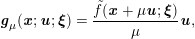 $$\begin{eqnarray}\boldsymbol{g}_{\unicode[STIX]{x1D707}}(\boldsymbol{x};\boldsymbol{u};\boldsymbol{\unicode[STIX]{x1D709}})=\displaystyle \frac{\tilde{f}(\boldsymbol{x}+\unicode[STIX]{x1D707}\boldsymbol{u};\boldsymbol{\unicode[STIX]{x1D709}})}{\unicode[STIX]{x1D707}}\boldsymbol{u},\end{eqnarray}$$
where
 $\boldsymbol{u}$
is drawn uniformly from the unit
 $n$
-dimensional sphere. That is, given a realization
 $\boldsymbol{\unicode[STIX]{x1D709}}\in \boldsymbol{\unicode[STIX]{x1D6EF}}$
, a stochastic gradient estimator based on a stochastic evaluation at the point
 $\boldsymbol{x}+\unicode[STIX]{x1D707}\boldsymbol{u}$
is computed via (4.10). For this method, and for general convex
 $f$
, Flaxman et al. (Reference Flaxman, Kalai and McMahan2005) demonstrate a WCC bound of type (4.9) in
 $O(n^{2}\unicode[STIX]{x1D716}^{-4})$
for general convex
 $f$
. For strongly convex
 $f$
, Flaxman et al. (Reference Flaxman, Kalai and McMahan2005) demonstrate a WCC bound of type (4.9) in
 $O(n^{2}\unicode[STIX]{x1D716}^{-3})$
. Various extensions of these results are given in Saha and Tewari (Reference Saha and Tewari2011), Dekel, Eldan and Koren (Reference Dekel, Eldan, Koren and Cortes2015) and Gasnikov et al. (Reference Gasnikov, Krymova, Lagunovskaya, Usmanova and Fedorenko2017). To the best of our knowledge, the best known upper bound on the WCC for smooth, strongly convex problems is in
 $O(n^{2}\unicode[STIX]{x1D716}^{-2})$
and the best known upper bound on the WCC for smooth, convex problems is in
 $O(n\unicode[STIX]{x1D716}^{-3})$
(Gasnikov et al.
Reference Gasnikov, Krymova, Lagunovskaya, Usmanova and Fedorenko2017).
Best known WCCs for
 $N_{\unicode[STIX]{x1D716}}$
, the number of evaluations required to bound (4.9), for one-point bandit feedback.
 $N_{\unicode[STIX]{x1D716}}$
is given only in terms of
 $n$
and
 $\unicode[STIX]{x1D716}$
. See text for the definition of
 $\unicode[STIX]{x1D6FD}$
-smooth; here
 $\unicode[STIX]{x1D6FD}>2$
. Method types include random search (RS), mirror descent (MD) and ellipsoidal.
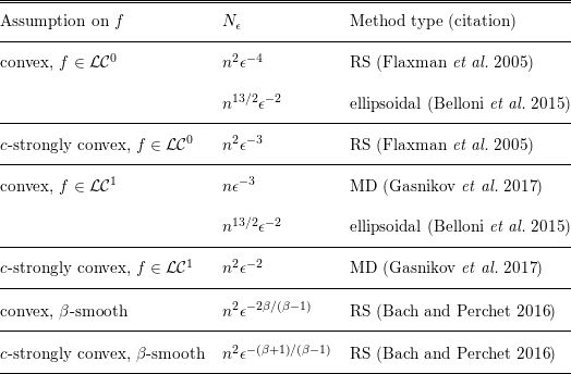
For the solution of (STOCH) when
 $\boldsymbol{\unicode[STIX]{x1D6FA}}=\mathbb{R}^{n}$
, Bach and Perchet (Reference Bach, Perchet and Feldman2016) analyse a method resembling Algorithm 6wherein the gradient-free oracle is chosen as
 $$\begin{eqnarray}\boldsymbol{g}_{\unicode[STIX]{x1D707}}(\boldsymbol{x};\boldsymbol{u};\boldsymbol{\unicode[STIX]{x1D709}}_{+},\boldsymbol{\unicode[STIX]{x1D709}}_{-})=\displaystyle \frac{\tilde{f}(\boldsymbol{x}+\unicode[STIX]{x1D707}\boldsymbol{u};\boldsymbol{\unicode[STIX]{x1D709}}_{+})-\tilde{f}(\boldsymbol{x}-\unicode[STIX]{x1D707}\boldsymbol{u};\boldsymbol{\unicode[STIX]{x1D709}}_{-})}{\unicode[STIX]{x1D707}}\boldsymbol{u},\end{eqnarray}$$
where
 $\boldsymbol{u}$
is again drawn uniformly from the unit
 $n$
-dimensional sphere. We remark that
 $\boldsymbol{\unicode[STIX]{x1D709}}_{+},\boldsymbol{\unicode[STIX]{x1D709}}_{-}\in \boldsymbol{\unicode[STIX]{x1D6EF}}$
in (4.11) are different realizations; this distinction will become particularly relevant in Section 4.2.2. For the solution of (STOCH) when
 $\boldsymbol{\unicode[STIX]{x1D6FA}}\subsetneq \mathbb{R}^{n}$
, Bach and Perchet (Reference Bach, Perchet and Feldman2016) also consider a gradient-free oracle like (4.10). Bach and Perchet (Reference Bach, Perchet and Feldman2016) are particularly interested in how the smoothness of
 $f$
can be exploited to improve complexity bounds in the one-point bandit feedback paradigm; they define a parameter
 $\unicode[STIX]{x1D6FD}$
and say that a function
 $f$
is
 $\unicode[STIX]{x1D6FD}$
-smooth provided
 $f$
is almost everywhere
 $(\unicode[STIX]{x1D6FD}-1)$
-times Lipschitz-continuously differentiable (a strictly weaker condition than assuming
 $f\in {\mathcal{L}}{\mathcal{C}}^{\unicode[STIX]{x1D6FD}-1}$
). When
 $\unicode[STIX]{x1D6FD}=2$
, Bach and Perchet (Reference Bach, Perchet and Feldman2016) recover similar results to those seen in Table 4.1 for when
 $f\in {\mathcal{L}}{\mathcal{C}}^{1}$
. When
 $\unicode[STIX]{x1D6FD}>2$
, however, in both the constrained and unconstrained case, Bach and Perchet (Reference Bach, Perchet and Feldman2016) prove a WCC result of type (4.9) in
 $O(n^{2}\unicode[STIX]{x1D716}^{2\unicode[STIX]{x1D6FD}/(1-\unicode[STIX]{x1D6FD})})$
when
 $f$
is convex and
 $\unicode[STIX]{x1D6FD}$
-smooth. Further assuming that
 $f$
is
 $c$
-strongly convex, Bach and Perchet (Reference Bach, Perchet and Feldman2016) prove a WCC result of type (4.9) in
 $O(n^{2}\unicode[STIX]{x1D716}^{(\unicode[STIX]{x1D6FD}+1)/(1-\unicode[STIX]{x1D6FD})}/c)$
. Notice that asymptotically, as
 $\unicode[STIX]{x1D6FD}\rightarrow \infty$
, this bound is in
 $O(n^{2}\unicode[STIX]{x1D716}^{-1}/c)$
. This asymptotic result is particularly important because it attains the lower bound on optimization error demonstrated by Shamir (Reference Shamir, Shalev-Shwartz and Steinwart2013) for strongly convex
 $\infty$
-smooth (quadratic)
 $f$
.
We also note that Bubeck et al. (Reference Bubeck, Lee and Eldan2017) conjecture that a particular kernel method can achieve a WCC of type (4.9) in
 $O(n^{3}\unicode[STIX]{x1D716}^{-2})$
for general convex functions. In light of well-known results in deterministic convex optimization, the WCCs summarized in Table 4.1 may be surprising. In particular, for any
 $c$
-strongly convex function
 $f\in {\mathcal{L}}{\mathcal{C}}^{1}$
, the best known WCC results are in
 $O(\unicode[STIX]{x1D716}^{-2})$
. We place particular emphasis on this result because it illustrates a gap between derivative-free and derivative-based optimization that is not just a factor of
 $n$
. In this particular one-point bandit feedback setting, there do not seem to exist methods that achieve the optimalFootnote
9
 $O(\unicode[STIX]{x1D716}^{-1})$
convergence rate attainable by gradient-based methods for smooth strongly convex stochastic optimization. Hu, Prashanth, György and Szepesvári (Reference Hu, Prashanth, György and Szepesvári2016) partially address this issue concerning one-point bandit feedback, which they refer to as ‘uncontrolled noise’. These observations motivated the study of two-point (multi-point) bandit feedback, which we will discuss in the next section, Section 4.2.2.
We further remark that every WCC in Table 4.1 has a polynomial dependence on the dimension
 $n$
, raising natural questions about the applicability of these methods in high-dimensional settings. Wang, Du, Balakrishnan and Singh (Reference Wang, Du, Balakrishnan, Singh, Storkey and Perez-Cruz2018) consider a mirror descent method employing a special gradient-free oracle computed via a compressed sensing technique. They prove a WCC of type (4.9) in
 $O(\log (d)^{3/2}n_{z}^{2}\unicode[STIX]{x1D716}^{-3})$
, under additional assumptions on derivative sparsity, most importantly, that for all
 $\boldsymbol{x}\in \boldsymbol{\unicode[STIX]{x1D6FA}}$
,
 $\Vert \unicode[STIX]{x1D6FB}f(\boldsymbol{x})\Vert _{0}\leq n_{z}$
for some
 $n_{z}$
. Thus, provided
 $n_{z}\ll n$
, the polynomial dependence on
 $n$
becomes a logarithmic dependence on
 $n$
, at the expense of a WCC with a strictly worse dependence on
 $\unicode[STIX]{x1D716}$
than
 $\unicode[STIX]{x1D716}^{-2}$
. In Section 5.2, we discuss methods that similarly exploit known sparsity of objective function derivatives.
In an extension of Algorithm 6, Chen (Reference Chen2015, Chapter 3) dynamically updates the difference parameter by exploiting knowledge of the changing variance of
 $\boldsymbol{\unicode[STIX]{x1D709}}$
.
4.2.2 Two-point (multi-point) bandit feedback
We now focus on the stochastic paradigm of two-point (or multi-point) bandit feedback. In this setting of bandit feedback, we do not encounter the same gaps in WCC results between derivative-free and derivative-based optimization that exist for one-point bandit feedback.
The majority of methods analysed in the two-point bandit feedback setting are essentially random-search methods of the form Algorithm 6. The gradient-free oracles from (3.1) in the two-point setting takes one of the two forms
 $$\begin{eqnarray}\begin{array}{@{}l@{}}\boldsymbol{g}_{\unicode[STIX]{x1D707}_{k}}(\boldsymbol{x};\boldsymbol{u};\boldsymbol{\unicode[STIX]{x1D709}})=\unicode[STIX]{x1D6FF}_{\text{f}}(\tilde{f}(\cdot ,\boldsymbol{\unicode[STIX]{x1D709}});\boldsymbol{x};\boldsymbol{u};\unicode[STIX]{x1D707}_{k})\boldsymbol{B}\boldsymbol{u},\quad \text{or}\\ \hat{\boldsymbol{g}}_{\unicode[STIX]{x1D707}_{k}}(\boldsymbol{x};\boldsymbol{u};\boldsymbol{\unicode[STIX]{x1D709}})=\unicode[STIX]{x1D6FF}_{\text{c}}(\tilde{f}(\cdot ,\boldsymbol{\unicode[STIX]{x1D709}});\boldsymbol{x};\boldsymbol{u};\unicode[STIX]{x1D707}_{k})\boldsymbol{B}\boldsymbol{u}.\end{array}\end{eqnarray}$$
The key observation in (4.12) is that
 $\boldsymbol{\unicode[STIX]{x1D709}}$
denotes a single realization used in the computation of both function values in the definitions of the oracles (see (2.28) and (2.29)). This assumption of ‘controllable realizations’ separates two-point bandit feedback from the more pessimistic one-point bandit feedback. This property of being able to recall a single realization
 $\boldsymbol{\unicode[STIX]{x1D709}}$
for two (or more) evaluations of
 $\tilde{f}$
is precisely why this setting of bandit feedback is called ‘two-point’ (or ‘multi-point’). This property will also be exploited in Section 6.1.
The early work of Agarwal, Dekel and Xiao (Reference Agarwal, Dekel, Xiao, Kalai and Mohri2010) directly addresses the discussed gap in WCC results and demonstrates that a random-search method resembling Algorithm 6, but applied in the two-point (or multi-point) setting as opposed to the one-point setting, attains a WCC of type (4.9) in
 $O(\unicode[STIX]{x1D716}^{-1})$
; this is a complexity result matching the optimal rate (in terms of
 $\unicode[STIX]{x1D716}$
-dependence) shown by Agarwal et al. (Reference Agarwal, Wainwright, Bartlett, Ravikumar and Bengio2009). See Table 4.2 for a summary of best known WCC results of type (4.9) for two-point bandit feedback methods.
Nesterov and Spokoiny (Reference Nesterov and Spokoiny2017) provide a WCC result for Algorithm 6using the stochastic gradient-free oracles (4.12), but strictly better WCCs have since been established. We also note that, in contrast with the gradient-free oracles of (3.1) in Section 3.1.2, the difference parameter
 $\unicode[STIX]{x1D707}$
is written as
 $\unicode[STIX]{x1D707}_{k}$
in (4.12), indicating that a selection for
 $\unicode[STIX]{x1D707}_{k}$
must be made in the
 $k$
th iteration. In the works that we discuss here,
 $\unicode[STIX]{x1D707}_{k}$
in (4.12) is either chosen as a constant sufficiently small or else
 $\unicode[STIX]{x1D707}_{k}\rightarrow 0$
at a rate typically of the order of
 $1/k$
. We also remark that many of the results discussed in this section trivially hold for deterministic convex problems, and can be seen as an extension of results concerning methods of the form of Algorithm 6.

Provided
 $f\in {\mathcal{L}}{\mathcal{C}}^{0}$
, the best known WCCs of type (4.9) (with variations in constants) can be found in Duchi, Jordan, Wainwright and Wibisono (Reference Duchi, Jordan, Wainwright and Wibisono2015), Gasnikov et al. (Reference Gasnikov, Krymova, Lagunovskaya, Usmanova and Fedorenko2017) and Shamir (Reference Shamir2017). These works consider variants of mirror-descent methods with approximate gradients given by estimators of the form (4.12); see Algorithm 7for a description of a basic mirror-descent method. Algorithm 7depends on the concept of a Bregman divergence
 $D_{\unicode[STIX]{x1D713}}$
, used in line 6of Algorithm 7to define a proximal-point subproblem. The Bregman divergence is defined by a function
 $\unicode[STIX]{x1D713}~:~\boldsymbol{\unicode[STIX]{x1D6FA}}\rightarrow \mathbb{R}$
, which is assumed to be
 $1$
-strongly convex with respect to the norm
 $\Vert \cdot \Vert _{p}$
. To summarize many findings in this area (Duchi et al.
Reference Duchi, Jordan, Wainwright and Wibisono2015, Gasnikov et al.
Reference Gasnikov, Krymova, Lagunovskaya, Usmanova and Fedorenko2017, Shamir Reference Shamir2017), if
 $\Vert \cdot \Vert _{q}$
is the dual norm to
 $\Vert \cdot \Vert _{p}$
(i.e.
 $p^{-1}+q^{-1}=1$
) where
 $p\in \{1,2\}$
and
 $R_{p}$
denotes the radius of the feasible set in the
 $\Vert \cdot \Vert _{p}$
-norm, then a bound on WCC of type (4.9) in
 $O(n^{2/q}R_{p}^{2}\unicode[STIX]{x1D716}^{-2})$
can be established for a method like Algorithm 7in the two-point feedback setting where
 $f\in {\mathcal{L}}{\mathcal{C}}^{0}$
. These WCCs for methods like Algorithm 7are responsible for the popularity of mirror-descent methods in machine learning. For many machine learning problems, solutions are typically sparse, and so, in some sense,
 $R_{1}\leq R_{2}$
. Thus, using a function
 $\unicode[STIX]{x1D713}$
that is
 $1$
-strongly convex with respect to the
 $\Vert \cdot \Vert _{1}$
-norm (e.g. simply letting
 $\unicode[STIX]{x1D713}=\Vert \cdot \Vert _{1}$
) may be preferable to
 $p=2$
, in both theory and practice.
Duchi et al. (Reference Duchi, Jordan, Wainwright and Wibisono2015) also provide an information-theoretic lower bound on convergence rates for any method in the (non-strongly) convex,
 $f\in {\mathcal{L}}{\mathcal{C}}^{0}$
, two-point feedback setting. This bound matches the best known WCCs up to constants, demonstrating that these results are tight. This lower bound is still of the order of
 $\unicode[STIX]{x1D716}^{-2}$
, matching the result of Agarwal et al. (Reference Agarwal, Wainwright, Bartlett, Ravikumar and Bengio2009) in
 $\unicode[STIX]{x1D716}$
-dependence in the case where
 $f\in {\mathcal{L}}{\mathcal{C}}^{0}$
. It is also remarkable that this result is only a factor of
 $\sqrt{n}$
worse than the bounds provided by Agarwal et al. (Reference Agarwal, Wainwright, Bartlett, Ravikumar and Bengio2009) for the derivative-based case, as opposed to the factor of
 $n$
that one may expect.
Best known WCCs of type (4.9) for two-point bandit feedback.
 $N_{\unicode[STIX]{x1D716}}$
is given only in terms of
 $n$
and
 $\unicode[STIX]{x1D716}$
. See text for the definition of
 $p,q$
.
 $R_{p}$
denotes the size of the feasible set in the
 $\Vert \cdot \Vert _{p}$
-norm. If
 $f$
is
 $c_{p}$
-strongly convex, then
 $f$
is strongly convex with respect to the
 $\Vert \cdot \Vert _{p}$
-norm with constant
 $c_{p}$
.
 $\unicode[STIX]{x1D70E}$
is the standard deviation on the gradient estimator
 $\boldsymbol{g}_{\unicode[STIX]{x1D707}}(\boldsymbol{x};\boldsymbol{u};\boldsymbol{\unicode[STIX]{x1D709}})$
(i.e.
 $\mathbb{E}_{\boldsymbol{\unicode[STIX]{x1D709}}}[\Vert \boldsymbol{g}_{\unicode[STIX]{x1D707}}(\boldsymbol{x};\boldsymbol{u};\boldsymbol{\unicode[STIX]{x1D709}})-\unicode[STIX]{x1D6FB}f(\boldsymbol{x})\Vert ^{2}]\leq \unicode[STIX]{x1D70E}^{2}$
). The Lipschitz constant of the gradient
 $L_{\text{g}}$
is defined by the
 $\Vert \cdot \Vert _{2}$
-norm.
 $\star$
denotes the additional assumption that
 $\mathbb{E}_{\boldsymbol{\unicode[STIX]{x1D709}}}[\Vert \boldsymbol{g}_{\unicode[STIX]{x1D707}}(\boldsymbol{x};\boldsymbol{u};\boldsymbol{\unicode[STIX]{x1D709}})\Vert ]<\infty$
. Method types include random search (RS), mirror descent (MD) and accelerated mirror descent (AMD).
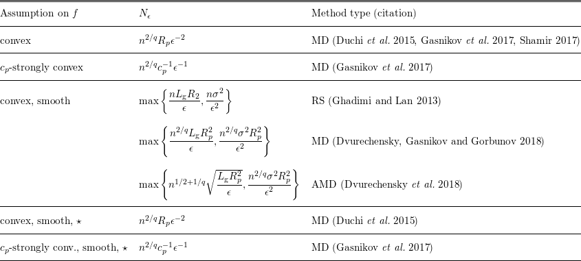
Additionally assuming
 $f(\boldsymbol{x})$
is strongly convex (but still assuming
 $f\in {\mathcal{L}}{\mathcal{C}}^{0}$
), Agarwal et al. (Reference Agarwal, Dekel, Xiao, Kalai and Mohri2010) prove, for a method like Algorithm 6, a WCC in
 $O(n^{2}\unicode[STIX]{x1D716}^{-1})$
. Using a method like Algorithm 7, Gasnikov et al. (Reference Gasnikov, Krymova, Lagunovskaya, Usmanova and Fedorenko2017) improve the dependence on
 $n$
in this WCC to
 $O(n^{2/q}c_{p}^{-1}\unicode[STIX]{x1D716}^{-1})$
, provided
 $f$
is
 $c_{p}$
-strongly convex with respect to
 $\Vert \cdot \Vert _{p}$
.
We now address the case where
 $f$
is convex and
 $f\in {\mathcal{L}}{\mathcal{C}}^{1}$
. Given an assumption that
 $\Vert \boldsymbol{g}_{\unicode[STIX]{x1D707}}(\boldsymbol{x};\boldsymbol{u};\boldsymbol{\unicode[STIX]{x1D709}})\Vert$
is uniformly bounded, Agarwal et al. (Reference Agarwal, Dekel, Xiao, Kalai and Mohri2010) demonstrate a WCC of type (4.9) in
 $O(n^{2}\unicode[STIX]{x1D716}^{-1})$
. Dropping this somewhat restrictive assumption on the gradient-free oracle and assuming instead that the oracle used in a method like Algorithm 6has bounded variance (i.e. the oracle satisfies
 $\mathbb{E}_{\boldsymbol{\unicode[STIX]{x1D709}}}[\Vert \boldsymbol{g}_{\unicode[STIX]{x1D707}}(\boldsymbol{x};\boldsymbol{u};\boldsymbol{\unicode[STIX]{x1D709}})-\unicode[STIX]{x1D6FB}f(\boldsymbol{x})\Vert ^{2}]\leq \unicode[STIX]{x1D70E}^{2}$
), Ghadimi and Lan (Reference Ghadimi and Lan2013) prove a WCC of a type similar to (4.9) (we avoid a discussion of randomized stopping) in
 $O(\max \{nL_{\text{g}}\Vert \boldsymbol{x}_{0}-\boldsymbol{x}_{\ast }\Vert \unicode[STIX]{x1D716}^{-1},n\unicode[STIX]{x1D70E}^{2}L_{g}\Vert \boldsymbol{x}_{0}-\boldsymbol{x}_{\ast }\Vert \unicode[STIX]{x1D716}^{-2}\})$
. We mention that Nesterov and Spokoiny (Reference Nesterov and Spokoiny2017) hinted at a similar WCC result, but with a strictly worse dependence on
 $n$
, and different assumptions on
 $\boldsymbol{\unicode[STIX]{x1D709}}$
.
5 Methods for structured objectives
The methods discussed in Sections 2 and 3 assume relatively little about the structure of the objective function
 $f$
beyond some differentiability required for analysis. Section 4 considered the case where
 $f$
is convex, which resulted, for example, in improved worst-case complexity results. In this section, we consider a variety of assumptions about additional known structure in
 $f$
(including non-linear least squares, sparse, composite and minimax-based functional forms) and methods designed to exploit this additional structure. Although problems in this section could be solved by the general-purpose methods discussed in Sections 2 and 3, practical gains should be expected by exploiting the additional structure.
5.1 Non-linear least squares
A frequently encountered objective in many applications of computational science, engineering and industry is
 $$\begin{eqnarray}f(\boldsymbol{x})=\displaystyle \frac{1}{2}\Vert \boldsymbol{F}(\boldsymbol{x})\Vert _{2}^{2}=\displaystyle \frac{1}{2}\mathop{\sum }_{i=1}^{p}F_{i}(\boldsymbol{x})^{2}.\end{eqnarray}$$
For example, data-fitting problems are commonly cast as (5.1); given data
 $y_{i}$
collected at design sites
 $\unicode[STIX]{x1D703}_{i}$
, one may need to estimate the parameters
 $\boldsymbol{x}$
of a non-linear model or simulation output that best fit the data. In this scenario,
 $F_{i}$
is represented by
 $F_{i}(\boldsymbol{x})=w_{i}(S_{i}(\unicode[STIX]{x1D73D};\boldsymbol{x})-y_{i})$
, which is a weighted residual between the simulation output
 $S_{i}$
and target data
 $y_{i}$
. In this way, objectives of the form (5.1) (and their correlated residual generalizations) encapsulate both the solution of non-linear equations and statistical estimation problems.
The methods of Zhang, Conn and Scheinberg (Reference Zhang, Conn and Scheinberg2010), Zhang and Conn (Reference Zhang and Conn2012) and Wild (Reference Wild and Terlaky2017) use the techniques of Section 2.2 to construct models of the individual
 $F_{i}$
(thereby obtaining a model of the Jacobian
 $\unicode[STIX]{x1D6FB}\boldsymbol{F}$
) in (5.1). These models are then used to generate search directions in a trust-region framework resembling the Levenberg–Marquardt method (Levenberg Reference Levenberg1944, Marquardt Reference Marquardt1963, Moré Reference Moré and Watson1978). The analysis by Zhang et al. (Reference Zhang, Conn and Scheinberg2010) and Zhang and Conn (Reference Zhang and Conn2012) demonstrates – under certain assumptions, such as
 $f(\boldsymbol{x}_{\ast })=0$
at an optimal solution
 $\boldsymbol{x}_{\ast }$
(i.e. that the associated data-fitting problem has zero residual) – that the resulting methods achieve the same local quadratic convergence rate does as the Levenberg–Marquardt method. POUNDERS is a trust-region-based method for minimizing objectives of the form (5.1) that uses a full Newton approach for each residual
 $F_{i}$
(Wild Reference Wild and Terlaky2017, Dener et al.
Reference Dener, Denchfield, Munson, Sarich, Wild, Benson and Curfman McInnes2018). Another model-based method (implemented in DFO-LS (Cartis, Fiala, Marteau and Roberts Reference Cartis, Fiala, Marteau and Roberts2018)) for minimizing functions of the form (5.1) – more closely resembling a Gauss–Newton method – is analysed by Cartis and Roberts (Reference Cartis and Roberts2017). Their method is shown to converge to stationary points of (5.1) even when
 $f(\boldsymbol{x}_{\ast })>0$
, at the expense of slightly weaker theoretical guarantees on the convergence rate.
Kelley (Reference Kelley, Sachs and Tichatschke2003) proposes a hybridization of a Gauss–Newton method with implicit filtering (Algorithm 4from Section 2.3.2) that estimates the Jacobian of
 $\boldsymbol{F}$
by building linear models of each component
 $F_{i}$
using central differences (2.29) with an algorithmically updated difference parameter. This hybrid method is shown to demonstrate superlinear convergence for zero-residual (i.e.
 $f(\boldsymbol{x}_{\ast })=0$
) problems.
Earlier methods also used the vector
 $F$
in order to more efficiently address objectives of the form (5.1). Spendley (Reference Spendley and Fletcher1969) develops a simplex-based algorithm that employs quadratic approximations obtained by interpolating the vector
 $F$
on the current simplex. Peckham (Reference Peckham1970) proposes an iterative process that refines models of each component of
 $F$
using between
 $n+1$
and
 $n+3+n/3$
points. Ralston and Jennrich (Reference Ralston and Jennrich1978) also develop derivative-free Gauss–Newton methods and highlight their performance relative to methods that do not exploit the structure in (5.1). Brown and Dennis, Jr (Reference Brown and Dennis1971) consider a variant of the Levenberg–Marquardt method that approximates gradients using appropriately selected difference parameters.
Li and Fukushima (Reference Li and Fukushima2000) analyse the convergence of a derivative-free line-search method when assuming that the square of the Jacobian (i.e.
 $\unicode[STIX]{x1D6FB}\boldsymbol{F}(\boldsymbol{x})^{\text{T}}\unicode[STIX]{x1D6FB}\boldsymbol{F}(\boldsymbol{x})$
) of (5.1) is positive-definite everywhere. Grippo and Sciandrone (Reference Grippo and Sciandrone2007) and La Cruz, Martínez and Raydan (Reference La Cruz, Martínez and Raydan2006) augment a non-monotone line-search method to incorporate information about
 $F$
in the case where
 $p=n$
in (5.1). Li and Li (Reference Li and Li2011) develop a line-search method that exploits a monotonicity property assumed about
 $\boldsymbol{F}$
. La Cruz (Reference La Cruz2014) and Morini, Porcelli and Toint (Reference Morini, Porcelli and Toint2018) address (5.1) in the case where simple convex constraints are present.
5.2 Sparse objective derivatives
In some applications, it is known that
 $$\begin{eqnarray}\unicode[STIX]{x1D6FB}^{2}f(\boldsymbol{x})_{ij}=\unicode[STIX]{x1D6FB}^{2}f(\boldsymbol{x})_{ji}=0\quad \text{for all}~(i,j)\in S,\end{eqnarray}$$
for all
 $\boldsymbol{x}\in \boldsymbol{\unicode[STIX]{x1D6FA}}$
, where the index set
 $S$
defines the sparsity pattern of the Hessian. Similarly, one can consider partially separable objectives of the form
 $$\begin{eqnarray}f(\boldsymbol{x})=\mathop{\sum }_{i=1}^{p}F_{i}(\boldsymbol{x})=\mathop{\sum }_{i=1}^{p}F_{i}(\{{\boldsymbol{x}_{j}\}}_{j\in S_{i}}),\end{eqnarray}$$
where each
 $F_{i}$
depends only on some subset of indices
 $S_{i}\subset \{1,2,\ldots ,n\}$
. The extreme cases of (5.3) are totally separable functions, where
 $p=n$
and
 $S_{i}=\{i\}$
for
 $i\in \{1,\ldots ,n\}$
. In this special case, (DET) reduces to the minimization of
 $n$
univariate functions.
Given the knowledge encoded in (5.2) and (5.3), derivative-free optimization methods need not consider interactions between certain components of
 $\boldsymbol{x}$
because they are known to be exactly zero. In the context of the model-based methods of Section 2.2, particularly when using quadratic models, using this knowledge amounts to dropping monomials in
 $\boldsymbol{\unicode[STIX]{x1D719}}(\boldsymbol{x})$
in (2.12) corresponding to the non-interacting
 $(i,j)$
pairs from (5.2). Intuitively, such an action reduces the degrees of freedom in (2.14) when building models, necessitating fewer function evaluations in the right-hand side of (2.14).
Colson and Toint (Reference Colson and Toint2005) propose a trust-region method for functions of the form (5.3) that builds and maintains separate fully linear models for the individual
 $F_{i}$
in an effort to use fewer objective function evaluations. Similarly, Colson and Toint (Reference Colson and Toint2001) propose a method for the case when
 $\unicode[STIX]{x1D6FB}^{2}f$
has a band or block structure that exploits knowledge when building models of the objective; the work of Colson and Toint (Reference Colson, Toint, Siddiqi and Kočvara2002) extends this work to general sparse objective Hessians. Bagirov and Ugon (Reference Bagirov and Ugon2006) develop an algorithm that exploits the fact that efficient discrete gradient estimates can be obtained for
 $f$
having the form (5.3).
In the context of pattern-search methods (discussed in Section 2.1.2), Price and Toint (Reference Price and Toint2006) exploit knowledge of
 $f$
having the form (5.3) to choose a particular stencil of search directions when forming a positive spanning set. In particular, the stencil is chosen as
 $\{\boldsymbol{e}_{1},\ldots ,\boldsymbol{e}_{n},\boldsymbol{e}_{n+1},\ldots ,\boldsymbol{e}_{n+p}\}$
, where
 $\{\boldsymbol{e}_{1},\ldots ,\boldsymbol{e}_{n}\}$
are the elementary basis vectors and
 $$\begin{eqnarray}\displaystyle \boldsymbol{e}_{n+i}=\mathop{\sum }_{j\in S_{i}}-\boldsymbol{e}_{j}, & & \displaystyle \nonumber\end{eqnarray}$$
for
 $i\in \{1,\ldots ,p\}$
. Frimannslund and Steihaug (Reference Frimannslund and Steihaug2010) also develop a DDS method for (5.3), with the search directions determined based on a smoothed quadratic formed from previously evaluated points.
Bandeira, Scheinberg and Vicente (Reference Bandeira, Scheinberg and Vicente2012) also assume that
 $\unicode[STIX]{x1D6FB}^{2}f(\boldsymbol{x})$
is sparse but do not assume knowledge of the sparsity structure (i.e.
 $S$
in (5.2) is not known). They develop a quadratic model-based trust-region method where the models are selected by a minimum
 $1$
-norm solution to an underdetermined interpolation system (2.14). Under certain assumptions on
 $f$
, if
 $n_{z}$
is the number of non-zeros in the (unknown) sparsity pattern for
 $\unicode[STIX]{x1D6FB}^{2}f$
, Bandeira et al. (Reference Bandeira, Scheinberg and Vicente2012) prove that
 $\boldsymbol{Y}$
in (2.14) must contain only
 $O((n_{z}+n)\log (n_{z}+n)\log (n))$
(as opposed to
 $O(n^{2})$
) randomly generated points in order to ensure that the constructed interpolation models are fully quadratic models of
 $f$
with high probability. This work motivated the analysis of randomized trust-region methods discussed in Section 3.3 because the random underdetermined interpolation models of Bandeira et al. (Reference Bandeira, Scheinberg and Vicente2012) satisfy the assumptions made in Bandeira et al. (Reference Bandeira, Scheinberg and Vicente2014).
In Section 4.2.1, we noted the work of Wang et al. (Reference Wang, Du, Balakrishnan, Singh, Storkey and Perez-Cruz2018), who used assumptions of gradient and Hessian sparsity (in particular,
 $\Vert \unicode[STIX]{x1D6FB}f(\boldsymbol{x})\Vert _{0}\leq n_{z}$
) to improve the reduce the dependence on
 $n$
in a WCC of type (4.9) from polynomial to logarithmic. Note that, similar to Bandeira et al. (Reference Bandeira, Scheinberg and Vicente2012), this is an assumption on knowing a universal bound (i.e. for all
 $\boldsymbol{x}\in \boldsymbol{\unicode[STIX]{x1D6FA}}$
) on the cardinality
 $\Vert \unicode[STIX]{x1D6FB}f(\boldsymbol{x})\Vert _{0}$
rather than the actual non-zero components. Under a similar sparsity assumption, Balasubramanian and Ghadimi (Reference Balasubramanian, Ghadimi and Bengio2018) consider the two-point bandit feedback setting discussed in Section 4.2.2 and show that a truncatedFootnote
10
version of the method proposed in Ghadimi and Lan (Reference Ghadimi and Lan2013) has a WCC of type (4.9) in
 $O(n_{z}\log (n)^{2}/\unicode[STIX]{x1D716}^{2})$
. Like the result of Wang et al. (Reference Wang, Du, Balakrishnan, Singh, Storkey and Perez-Cruz2018), this WCC result also exhibits a logarithmic dependence on
 $n$
, provided
 $n_{z}\ll n$
. As we will discuss in Section 6.4, Ghadimi and Lan (Reference Ghadimi and Lan2013) analyse a method resembling Algorithm 6to be applied to non-convex
 $f$
in (STOCH). Balasubramanian and Ghadimi (Reference Balasubramanian, Ghadimi and Bengio2018) prove that the unaltered method of Ghadimi and Lan (Reference Ghadimi and Lan2013) applied to problems in this sparse setting achieves a WCC of type
 $$\begin{eqnarray}\mathbb{E}_{}[\Vert \unicode[STIX]{x1D6FB}f(\boldsymbol{x}_{k})\Vert ]\leq \unicode[STIX]{x1D716},\end{eqnarray}$$
in
 $O(n_{z}^{2}\log (n)^{2}\unicode[STIX]{x1D716}^{-4})$
; this WCC result once again eliminates a polynomial dependence on
 $n$
that would otherwise exist in a non-sparse setting. This WCC result, however, maintains the same
 $\unicode[STIX]{x1D716}$
-dependence as the method of Ghadimi and Lan (Reference Ghadimi and Lan2013) in the non-sparse setting; in this sense, the method of Ghadimi and Lan (Reference Ghadimi and Lan2013) is ‘automatically’ tuned for the sparse setting.
5.3 Composite non-smooth optimization
Sometimes, the objective
 $f$
in (DET) is known to be non-smooth. Often, one has knowledge about the form of non-smoothness present in the objective, and we discuss methods that exploit specific forms of non-smoothness in this section. For methods that do not access any structural information when optimizing non-smooth functions
 $f$
, see Sections 2.1.2 and2.3.
We define composite non-smooth functions as those of the form
 $$\begin{eqnarray}f(\boldsymbol{x})=h(\boldsymbol{F}(\boldsymbol{x})),\end{eqnarray}$$
where
 $h:\mathbb{R}^{p}\rightarrow \mathbb{R}$
is a non-smooth function (in contrast to smooth
 $h$
such as the sum of squares in (5.1)), and
 $\boldsymbol{F}~:~\mathbb{R}^{n}\rightarrow \mathbb{R}^{p}$
is continuously differentiable. In some of the works we cite, the definition of a composite non-smooth objective may include an additional smooth function
 $g$
so that the objective function has the form
 $f(\boldsymbol{x})+g(\boldsymbol{x})$
, but we omit a discussion of this for the sake of focusing on the non-smooth aspect in (5.5).
5.3.1 Convex
$h$

When
 $h$
in (5.5) is convex (note that
 $f$
may still be non-convex due to non-convexity in
 $\boldsymbol{F}$
), one thrust of research extends the techniques in derivative-based composite non-smooth optimization; see the works of Yuan (Reference Yuan1985) and Fletcher (Reference Fletcher1987, Chapter 14). For example, Yuan (Reference Yuan1985) use derivatives to construct convex first-order approximations of
 $f$
near
 $\boldsymbol{x}$
,
 $$\begin{eqnarray}\ell (\boldsymbol{x}+\boldsymbol{s})=h(\boldsymbol{F}(\boldsymbol{x})+\unicode[STIX]{x1D6FB}\boldsymbol{F}(\boldsymbol{x})\boldsymbol{s}),\end{eqnarray}$$
where
 $\unicode[STIX]{x1D6FB}\boldsymbol{F}$
denotes the Jacobian of
 $\boldsymbol{F}$
; see Hare (Reference Hare2017) for properties of such approximations in the derivative-free setting. By replacing
 $\unicode[STIX]{x1D6FB}\boldsymbol{F}$
in (5.6) with the matrix
 $\boldsymbol{M}(\boldsymbol{x}_{k})$
containing the gradients of a fully linear approximation to
 $\boldsymbol{F}$
at
 $\boldsymbol{x}_{k}$
, Grapiglia, Yuan and Yuan (Reference Grapiglia, Yuan and Yuan2016) and Garmanjani et al. (Reference Garmanjani, Jùdice and Vicente2016) independently analyse a model-based trust-region method similar to Algorithm 3from Section 2.2.4 that uses the non-smooth trust-region subproblem

Note that only
 $\boldsymbol{F}$
is assumed to be a black-box; these methods exploit the fact that
 $h$
is convex with a known form in order to appropriately solve (5.6). Both Grapiglia et al. (Reference Grapiglia, Yuan and Yuan2016) and Garmanjani et al. (Reference Garmanjani, Jùdice and Vicente2016) use the stationarity measure of Yuan (Reference Yuan1985) in their analysis,
 $$\begin{eqnarray}\unicode[STIX]{x1D6F9}(\boldsymbol{x})=\ell (\boldsymbol{x})-\min _{\Vert \boldsymbol{s}\Vert \leq 1}\ell (\boldsymbol{x}+\boldsymbol{s}),\end{eqnarray}$$
for which it is known that
 $\unicode[STIX]{x1D6F9}(\boldsymbol{x}_{\ast })=0$
if and only if
 $\boldsymbol{x}_{\ast }$
is a critical point of
 $f$
in the sense that
 $\ell (\boldsymbol{x}_{\ast })\leq \ell (\boldsymbol{x}_{\ast }+\boldsymbol{s})$
for all
 $\boldsymbol{s}\in \mathbb{R}^{n}$
. Worst-case complexity results that bound the effort required to attain
 $\Vert \unicode[STIX]{x1D6F9}(\boldsymbol{x}_{k})\Vert \leq \unicode[STIX]{x1D716}$
are included in Table A.1.
Methods using the local approximation (5.6) require convexity of
 $h$
in order for
 $\unicode[STIX]{x1D6F9}$
in (5.8) to be interpreted as a stationarity measure. From a practical perspective, the form of
 $h$
directly affects the difficulty of solving the trust-region subproblem. Grapiglia et al. (Reference Grapiglia, Yuan and Yuan2016) demonstrate this approach on a collection of problems of the form
 $$\begin{eqnarray}f(\boldsymbol{x})=\max _{i=1,\ldots ,p}F_{i}(\boldsymbol{x}),\end{eqnarray}$$
where each
 $F_{i}$
is assumed smooth. Garmanjani et al. (Reference Garmanjani, Jùdice and Vicente2016) test their method on a collection of problems of the form
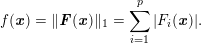 $$\begin{eqnarray}f(\boldsymbol{x})=\Vert \boldsymbol{F}(\boldsymbol{x})\Vert _{1}=\mathop{\sum }_{i=1}^{p}|F_{i}(\boldsymbol{x})|.\end{eqnarray}$$
For objectives of the form (5.9) or (5.10), the associated trust-region subproblems (5.7) can be cast as linear programs when the
 $\infty$
-norm defines the trust region. (An early example of such an approach appears in Madsen (Reference Madsen, Balinski and Wolfe1975), where linear approximations to each
 $F_{i}$
in (5.9) are constructed.) Although more general convex
 $h$
could fit into this framework, one must be wary of the difficulty of the resulting subproblems.
Direct-search methods have also been adapted for composite non-smooth functions of specific forms. In these variants, knowledge of
 $h$
in (5.5) informs the selection of search directions in a manner similar to that described in Section 5.2. Ma and Zhang (Reference Ma and Zhang2009) and Bogani, Gasparo and Papini (Reference Bogani, Gasparo and Papini2009) consider the cases of
 $f$
of the form (5.9) and (5.10), respectively.
Objectives of the form (5.9) are also addressed by Hare, Planiden and Sagastizábal (Reference Hare, Planiden and Sagastizábal2019), who develop an algorithm that decomposes such problems into orthogonal subspaces associated with directions of non-smoothness and directions of smoothness. The resulting derivative-free
 $VU$
-algorithm employs model-based estimates of gradients to form and update this decomposition (Hare Reference Hare2014). Liuzzi, Lucidi and Sciandrone (Reference Liuzzi, Lucidi and Sciandrone2006) address finite minimax problems by converting the original problem into a smooth problem using an exponential penalty function. Their DDS method adjusts the penalty parameter via a rule that depends on the current step size in order to guarantee convergence to a Clarke stationary point.
Approximate gradient-sampling methods are developed and analysed by Hare and Macklem (Reference Hare and Macklem2013) and Hare and Nutini (Reference Hare and Nutini2013) for the finite minimax problem (5.9). These methods effectively exploit the subdifferential structure of
 $h(\boldsymbol{y})=\max _{i=1,\ldots ,p}y_{i}$
and employ derivative-free approximations of each
 $\unicode[STIX]{x1D6FB}F_{i}(\boldsymbol{x})$
. Larson, Menickelly and Wild (Reference Larson, Menickelly and Wild2016) propose a variant of gradient sampling, called manifold sampling, for objectives of the form (5.10). Unlike (approximate) gradient sampling, manifold sampling does not depend on a random sample of points to estimate the
 $\unicode[STIX]{x1D716}$
-subdifferential.
5.3.2 Non-convex
$h$

When
 $h$
is non-convex, minimization of (5.5) is considerably more challenging than when
 $h$
is convex. Few methods exist that exploit the structure of non-convex
 $h$
. One of the many challenges is that the model in (5.6) may no longer be an underestimator of
 $h$
. Khan et al. (Reference Khan, Larson and Wild2018) propose a manifold sampling method for piecewise linear
 $h$
; in contrast to the previously discussed methods, this method does not require that
 $h$
be convex. Other methods applicable for non-convex
 $h$
employ smoothing functions.
As mentioned in Section 2.1.2, the worst-case complexity of DDS methods applied to non-smooth (Lipschitz-continuous) objective functions is difficult to analyse. The reason that DDS methods generate an asymptotically dense set of polling directions is to ensure that no descent directions exist. An exception to this generality, however, is functions for which an appropriate smoothing function exists. Given a locally Lipschitz-continuous
 $f$
, we say that
 $f_{\unicode[STIX]{x1D707}}:\mathbb{R}^{n}\rightarrow \mathbb{R}$
is a smoothing function for
 $f$
provided that for any
 $\unicode[STIX]{x1D707}\in (0,\infty )$
,
 $f_{\unicode[STIX]{x1D707}}$
is continuously differentiable and that
 $$\begin{eqnarray}\displaystyle \lim _{\boldsymbol{z}\rightarrow \boldsymbol{x},\unicode[STIX]{x1D707}\rightarrow 0^{+}}f_{\unicode[STIX]{x1D707}}(\boldsymbol{z})=f(\boldsymbol{x}), & & \displaystyle \nonumber\end{eqnarray}$$
for all
 $\boldsymbol{x}\in \mathbb{R}^{n}$
.
Thus, if a smoothing function
 $f_{\unicode[STIX]{x1D707}}$
exists for
 $f$
, it is natural to iteratively apply a method for smooth unconstrained optimization to obtain approximate solutions
 $\boldsymbol{x}_{k}$
to
 $\min _{\boldsymbol{x}}f_{\unicode[STIX]{x1D707}_{k}}(\boldsymbol{x})$
while decreasing
 $\unicode[STIX]{x1D707}_{k}$
. We roughly prescribe such a smoothing method in Algorithm 8.

Garmanjani and Vicente (Reference Garmanjani and Vicente2012) consider the DDS framework analysed by Vicente (Reference Vicente2013) as the method
 $\mathfrak{M}$
in Algorithm 8.They terminate
 $\mathfrak{M}$
when the step-size parameter
 $\unicode[STIX]{x1D6FC}$
of Algorithm 2is sufficiently small, where the notion of sufficiently small scales with
 $\unicode[STIX]{x1D707}_{k}$
in Algorithm 8.Garmanjani and Vicente (Reference Garmanjani and Vicente2012) prove a first-order stationarity result of the form
 $$\begin{eqnarray}\liminf _{k\rightarrow \infty }\Vert \unicode[STIX]{x1D6FB}f_{\unicode[STIX]{x1D707}_{k}}(\boldsymbol{x}_{k})\Vert =0.\end{eqnarray}$$
Under certain assumptions (for instance, that
 $h$
satisfies some regularity conditions at
 $\boldsymbol{F}(\boldsymbol{x}_{\ast })$
) this first-order stationarity result is equivalent to
 $0\in \unicode[STIX]{x2202}f(\boldsymbol{x}_{\ast })$
; that is,
 $\boldsymbol{x}_{\ast }$
is Clarke stationary.
Garmanjani and Vicente (Reference Garmanjani and Vicente2012) consider the decrease to be sufficient in line 4of Algorithm 1if
 $f(\boldsymbol{p}_{i})<f(\boldsymbol{x})-c_{1}\unicode[STIX]{x1D6FC}^{3/2}$
for some
 $c_{1}>0$
. If, furthermore,
 $\mathfrak{M}$
terminates in each iteration of Algorithm 8when
 $\unicode[STIX]{x1D6FC}<c_{2}\unicode[STIX]{x1D707}_{k}^{2}$
for some
 $c_{2}>0$
, then an upper bound on the number of function evaluations needed to obtain
 $$\begin{eqnarray}\Vert \unicode[STIX]{x1D6FB}f_{\unicode[STIX]{x1D707}_{\ast }}(\boldsymbol{x}_{k})\Vert \leq \unicode[STIX]{x1D716},\end{eqnarray}$$
for
 $\unicode[STIX]{x1D716}\in (0,1)$
and
 $\unicode[STIX]{x1D707}_{\ast }\in O(n^{-1/2}\unicode[STIX]{x1D716})$
, is in
 $O(\unicode[STIX]{x1D716}^{-3})$
; see Table A.1. We note that while the sequence of smoothing parameters
 $\unicode[STIX]{x1D707}_{k}$
induces a type of limiting behaviour of the gradients (as seen in (5.12)) returned by the method
 $\mathfrak{M}$
used in Algorithm 8, this still does not necessarily recover elements of the Clarke subdifferential of
 $f$
. The smoothing functions
 $f_{\unicode[STIX]{x1D707}_{k}}$
must satisfy an additional gradient consistency property in order for Algorithm 8to produce a sequence of points
 $\boldsymbol{x}_{k}$
converging to Clarke stationary points (Rockafellar and Wets Reference Rockafellar and Wets2009, Theorem 9.67).
Garmanjani et al. (Reference Garmanjani, Jùdice and Vicente2016) consider the use of a model-based trust-region method
 $\mathfrak{M}$
in Algorithm 8. The authors demonstrate the first-order convergence result (5.11); they also prove the same WCC as is proved by Garmanjani and Vicente (Reference Garmanjani and Vicente2012).
5.4 Bilevel and general minimax problems
Bilevel optimization addresses problems where a lower-level objective is embedded within an upper-level problem. Bilevel problems take the form
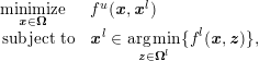
where
 $f^{u}:\boldsymbol{\unicode[STIX]{x1D6FA}}\subseteq \mathbb{R}^{n}\rightarrow \mathbb{R}$
and
 $f^{l}:\boldsymbol{\unicode[STIX]{x1D6FA}}^{l}\subseteq \mathbb{R}^{n^{l}}\rightarrow \mathbb{R}$
. Conn and Vicente (Reference Conn and Vicente2012) propose a model-based trust-region method for solving (5.14) in the absence of derivative information. They show how to obtain approximations of the upper-level objective by solving the lower-level problem to sufficient accuracy. Mersha and Dempe (Reference Mersha and Dempe2011) and Zhang and Lin (Reference Zhang and Lin2014) develop DDS-based algorithms for (5.13) under particular assumptions (e.g. strict convexity of the lower-level problem).
A special case of (5.13) is when
 $f^{l}=-f^{u}$
, which results in the minimax problem (DET), where the objective is given by a maximization:
 $$\begin{eqnarray}f(\boldsymbol{x})=\max _{\boldsymbol{x}^{l}\in \boldsymbol{\unicode[STIX]{x1D6FA}}^{l}}f^{l}(\boldsymbol{x},\boldsymbol{x}^{l}).\end{eqnarray}$$
In contrast to the finite minimax problem (5.9), the objective in (5.14) involves a potentially infinite set
 $\boldsymbol{\unicode[STIX]{x1D6FA}}^{l}$
.
Bertsimas, Nohadani and Teo (Reference Bertsimas, Nohadani and Teo2010) and Bertsimas and Nohadani (Reference Bertsimas and Nohadani2010) consider (5.14) when exact gradients of
 $f^{l}$
may not be available. The authors assume that approximate gradients of
 $f^{l}$
are available and propose methods with convergence analysis restricted to functions
 $f$
in (5.14) that are convex in
 $\boldsymbol{x}$
. Ciccazzo et al. (Reference Ciccazzo, Latorre, Liuzzi, Lucidi and Rinaldi2015) and Latorre, Habal, Graeb and Lucidi (Reference Latorre, Habal, Graeb and Lucidi2019) develop derivative-free methods that employ approximate solutions of the inner problem in (5.14). Menickelly and Wild (Reference Menickelly and Wild2019) also consider (5.14) and develop a derivative-free method of outer approximations for more general
 $f$
. Their analysis shows that the resulting limit points are Clarke stationary for
 $f$
.
6 Methods for stochastic optimization
We now turn our attention to methods for solving the stochastic optimization problem (STOCH). In Section 4.2, we considered the case where
 $f(\boldsymbol{x})=\mathbb{E}_{\boldsymbol{\unicode[STIX]{x1D709}}}[\tilde{f}(\boldsymbol{x};\boldsymbol{\unicode[STIX]{x1D709}})]$
is convex. In this section, we lift the assumption of convexity to consider a more general class of stochastic functions
 $\tilde{f}$
.
In general, the analysis of methods for stochastic optimization requires assumptions on the random variable
 $\boldsymbol{\unicode[STIX]{x1D709}}$
. In this section, we use the convention that
 $\boldsymbol{\unicode[STIX]{x1D709}}\sim \boldsymbol{\unicode[STIX]{x1D6EF}}$
denotes that the random variable
 $\boldsymbol{\unicode[STIX]{x1D709}}$
is from a distribution
 $\boldsymbol{\unicode[STIX]{x1D6EF}}$
and that
 $\boldsymbol{\unicode[STIX]{x1D709}}\in \boldsymbol{\unicode[STIX]{x1D6EF}}$
refers to a random variable in the support of this distribution. Frequently, realizations
 $\boldsymbol{\unicode[STIX]{x1D709}}\sim \boldsymbol{\unicode[STIX]{x1D6EF}}$
are assumed to be independent and identically distributed (i.i.d.). Throughout this section, we assume that
 $\mathbb{E}_{\boldsymbol{\unicode[STIX]{x1D709}}}[\tilde{f}(\boldsymbol{x};\boldsymbol{\unicode[STIX]{x1D709}})]$
exists for each
 $\boldsymbol{x}\in \boldsymbol{\unicode[STIX]{x1D6FA}}$
and
 $f(\boldsymbol{x})=\mathbb{E}_{\boldsymbol{\unicode[STIX]{x1D709}}}[\tilde{f}(\boldsymbol{x};\boldsymbol{\unicode[STIX]{x1D709}})]$
; that is, the objective of (STOCH) is well-defined. Another common assumption in the stochastic optimization literature is that some bound on the variance of
 $\tilde{f}(\boldsymbol{x};\boldsymbol{\unicode[STIX]{x1D709}})$
is assumed, that is,
 $$\begin{eqnarray}\mathbb{E}_{\boldsymbol{\unicode[STIX]{x1D709}}}[(\tilde{f}(\boldsymbol{x};\boldsymbol{\unicode[STIX]{x1D709}})-f(\boldsymbol{x}))^{2}]<\unicode[STIX]{x1D70E}^{2}<\infty \quad \text{for all }\boldsymbol{x}\in \boldsymbol{\unicode[STIX]{x1D6FA}}.\end{eqnarray}$$
If, for a given
 $\boldsymbol{x}$
,
 $\unicode[STIX]{x1D6FB}_{\boldsymbol{x}}\tilde{f}(\boldsymbol{x};\boldsymbol{\unicode[STIX]{x1D709}})$
exists for each
 $\boldsymbol{\unicode[STIX]{x1D709}}\in \boldsymbol{\unicode[STIX]{x1D6EF}}$
, then under certain regularity conditions it follows that
 $\unicode[STIX]{x1D6FB}f(\boldsymbol{x})=\mathbb{E}_{\boldsymbol{\unicode[STIX]{x1D709}}}[\unicode[STIX]{x1D6FB}_{\boldsymbol{x}}\tilde{f}(\boldsymbol{x};\boldsymbol{\unicode[STIX]{x1D709}})]$
; one such regularity condition is that
 $$\begin{eqnarray}\displaystyle \tilde{f}(\cdot ;\boldsymbol{\unicode[STIX]{x1D709}})\text{ is }L_{\tilde{f}(\cdot ;\boldsymbol{\unicode[STIX]{x1D709}})}\text{-Lipschitz-continuous and }\mathbb{E}_{\boldsymbol{\unicode[STIX]{x1D709}}}[L_{\tilde{f}(\cdot ;\boldsymbol{\unicode[STIX]{x1D709}})}]<\infty . & & \displaystyle \nonumber\end{eqnarray}$$
We note that when first-order information is available, the assumption (6.1) is often replaced by an assumption on the variance of the expected gradient norm; see e.g. Bottou, Curtis and Nocedal (Reference Bottou, Curtis and Nocedal2018, Assumption 4.3). In this setting, a key class of methods for (STOCH) are stochastic approximation (SA) methods; see the paper proposing SA methods by Robbins and Monro (Reference Robbins and Monro1951) and a survey of modern SA methods (often also referred to as ‘stochastic gradient’ methods when first-order information is available) by Bottou et al. (Reference Bottou, Curtis and Nocedal2018). Here we focus on situations where no objective derivative information is available; that is, stochastic gradient methods are not directly applicable. That said, some of the work we discuss attempts to approximate stochastic gradients, which are then used in an SA framework. As discussed in Section 1, we will not address global optimization methods, such as Bayesian optimization.Footnote 11
Section 6.1 discusses stochastic approximation methods, and Section 6.2 presents direct-search methods for stochastic optimization. In Section 6.3 we highlight modifications to derivative-free model-based methods to address (STOCH), and in Section 6.4 we discuss bandit methods for (non-convex) stochastic optimization.
6.1 Stochastic and sample-average approximation
One of the first analysed approaches for solving (STOCH) is the method of Kiefer and Wolfowitz (Reference Kiefer and Wolfowitz1952), inspired by the SA method of Robbins and Monro (Reference Robbins and Monro1951). We state the basic Kiefer–Wolfowitz framework in Algorithm 9.Since Kiefer and Wolfowitz (Reference Kiefer and Wolfowitz1952) consider only univariate problems, Algorithm 9is in fact the multivariate extension first of Blum (Reference Blum1954b
). In Algorithm 9,
 $\unicode[STIX]{x1D6FB}f(\boldsymbol{x}_{k})$
is approximated by observing realizations of
 $\tilde{f}$
using central differences. That is,
 $\unicode[STIX]{x1D6FB}f(\boldsymbol{x}_{k})$
is approximated by
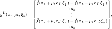 $$\begin{eqnarray}\boldsymbol{g}^{\text{K}}(\boldsymbol{x}_{k};\unicode[STIX]{x1D707}_{k};\boldsymbol{\unicode[STIX]{x1D709}}_{k})=\left[\begin{array}{@{}c@{}}\displaystyle \frac{\tilde{f}(\boldsymbol{x}_{k}+\unicode[STIX]{x1D707}_{k}\boldsymbol{e}_{1};\boldsymbol{\unicode[STIX]{x1D709}}_{1}^{+})-\tilde{f}(\boldsymbol{x}_{k}-\unicode[STIX]{x1D707}_{k}\boldsymbol{e}_{1};\boldsymbol{\unicode[STIX]{x1D709}}_{1}^{-})}{2\unicode[STIX]{x1D707}_{k}}\\ \vdots \\ \displaystyle \frac{\tilde{f}(\boldsymbol{x}_{k}+\unicode[STIX]{x1D707}_{k}\boldsymbol{e}_{n};\boldsymbol{\unicode[STIX]{x1D709}}_{n}^{+})-\tilde{f}(\boldsymbol{x}_{k}-\unicode[STIX]{x1D707}_{k}\boldsymbol{e}_{n};\boldsymbol{\unicode[STIX]{x1D709}}_{n}^{-})}{2\unicode[STIX]{x1D707}_{k}}\end{array}\right]\!,\end{eqnarray}$$
where
 $\unicode[STIX]{x1D707}_{k}>0$
is a difference parameter,
 $\boldsymbol{e}_{i}$
is the
 $i$
th elementary basis vector, and
 $2n$
realizations
 $\boldsymbol{\unicode[STIX]{x1D709}}\sim \boldsymbol{\unicode[STIX]{x1D6EF}}$
are employed. The next point
 $\boldsymbol{x}_{k+1}$
is then set to be
 $\boldsymbol{x}_{k}-\unicode[STIX]{x1D6FC}_{k}\boldsymbol{g}^{\text{K}}(\boldsymbol{x}_{k};\unicode[STIX]{x1D707}_{k};\boldsymbol{\unicode[STIX]{x1D709}}_{k})$
, where
 $\unicode[STIX]{x1D6FC}_{k}>0$
is a step-size parameter. As in Section 3, we note that
 $\boldsymbol{x}_{k+1}$
is a random variable that depends on the filtration generated by the method before
 $\boldsymbol{x}_{k+1}$
is realized; this will be the case throughout this section. In the SA literature, the sequences
 $\{\unicode[STIX]{x1D6FC}_{k}\}$
and
 $\{\unicode[STIX]{x1D707}_{k}\}$
are often referred to as gain sequences.

Because evaluation of the function
 $f$
requires computing an expectation (and in contrast to the primarily monotone algorithms in Section 2), stochastic optimization methods generally do not monotonically decrease
 $f$
. This is exemplified by Algorithm 9, which updates
 $\boldsymbol{x}_{k+1}$
without considering the value of
 $\tilde{f}(\boldsymbol{x}_{k+1};\boldsymbol{\unicode[STIX]{x1D709}})$
for any realization of
 $\boldsymbol{\unicode[STIX]{x1D709}}$
.
Historically, Algorithm 9has been analysed by a community more concerned with stochastic processes than with optimization. Hence, convergence results differ from those commonly found in the optimization literature. For example, many results in the SA literature consider a continuation of the dynamics of Algorithm 9applied to the deterministic
 $f$
as an ordinary differential equation (ODE) in terms of
 $\boldsymbol{x}(t):\mathbb{R}\rightarrow \mathbb{R}^{n}$
. That is, they consider
 $$\begin{eqnarray}\displaystyle \displaystyle \frac{\text{d}\boldsymbol{x}}{\text{d}t}=-\unicode[STIX]{x1D6FB}f(\boldsymbol{x}),\quad \boldsymbol{x}=\boldsymbol{x}(t). & & \displaystyle \nonumber\end{eqnarray}$$
and define the set of fixed points of the ODE,
 $\boldsymbol{S}=\{\boldsymbol{x}~:~\unicode[STIX]{x1D6FB}f(\boldsymbol{x})=0\}.$
Many convergence results then demonstrate that the continuation
 $\boldsymbol{x}(t)$
satisfies
 $\boldsymbol{x}(t)\rightarrow \boldsymbol{S}$
with probability one as the continuous iteration counter
 $t\rightarrow \infty$
; see Kushner and Yin (Reference Kushner and Yin2003) for a complete treatment of such ODE results.
In order to prove that the sequence of points
 $\boldsymbol{x}_{k}$
generated by Algorithm 9converges almost surely (i.e. with probability one), conditions must be placed on the objective function, step sizes and difference parameters. In the SA literature there is no single consistent set of conditions, but there are nearly always conditions on the sequence of step sizes
 $\{\unicode[STIX]{x1D6FC}_{k}\}$
requiring
 $\unicode[STIX]{x1D6FC}_{k}\rightarrow 0$
and
 $\sum _{k}\unicode[STIX]{x1D6FC}_{k}=\infty$
. Intuitively, this divergence condition ensures that any point in the domain
 $\boldsymbol{\unicode[STIX]{x1D6FA}}$
can be reached, independent of the history of iterations. As one example of convergence conditions, Bhatnagar, Prasad and Prashanth (Reference Bhatnagar, Prasad and Prashanth2013) prove almost sure convergence of Algorithm 9under the following assumptions (simplified for presentation).
(1) The sequences of step sizes and difference parameters satisfy
$\unicode[STIX]{x1D6FC}_{k}>0$
,
$\unicode[STIX]{x1D707}_{k}>0$
,
$\unicode[STIX]{x1D6FC}_{k}\rightarrow 0$
,
$\unicode[STIX]{x1D707}_{k}\rightarrow 0$
,
$\sum _{k}\unicode[STIX]{x1D6FC}_{k}=\infty$
and
$\sum _{k}\unicode[STIX]{x1D6FC}_{k}^{2}\unicode[STIX]{x1D707}_{k}^{-2}<\infty$
.(2) The realizations
$\boldsymbol{\unicode[STIX]{x1D709}}\sim \boldsymbol{\unicode[STIX]{x1D6EF}}$
are i.i.d. and the distribution
$\boldsymbol{\unicode[STIX]{x1D6EF}}$
has a finite second moment.(3) The function
$f$
is in
${\mathcal{L}}{\mathcal{C}}^{1}$
.(4)
$\sup _{k}\{\Vert \boldsymbol{x}_{k}\Vert \}<\infty$
with probability one.






Similar assumptions on algorithms of the form Algorithm 9appear throughout the SA literature (Blum Reference Blum1954a
, Derman Reference Derman1956, Sacks Reference Sacks1958, Fabian Reference Fabian1971, Kushner and Huang Reference Kushner and Huang1979, Ruppert Reference Ruppert, Ghosh and Sen1991, Spall Reference Spall2005). Convergence of Algorithm 9under similar assumptions to those above, but with the modification that
 $\unicode[STIX]{x1D707}_{k}$
is fixed in every iteration to a sufficiently small constant (that scales inversely with
 $L_{\text{g}}$
), is additionally demonstrated by Bhatnagar et al. (Reference Bhatnagar, Prasad and Prashanth2013).
In terms of WCCs, the convergence rates that have been historically derived for Algorithm 9are also non-standard for optimization. In particular, results concerning convergence rates are typically shown as a convergence in distribution (Durrett Reference Durrett2010, Chapter 3.2): given a fixed
 $\boldsymbol{x}_{\ast }\in \boldsymbol{S}$
,
 $$\begin{eqnarray}\displaystyle \frac{1}{k^{\unicode[STIX]{x1D6FE}}}(\boldsymbol{x}_{k}-\boldsymbol{x}_{\ast })\rightarrow {\mathcal{N}}(\mathbf{0},\boldsymbol{B}),\end{eqnarray}$$
where
 $\unicode[STIX]{x1D6FE}>0$
and
 $\boldsymbol{B}$
is a covariance matrix, the entries of which depend on algorithmic parameters and
 $\unicode[STIX]{x1D6FB}^{2}f(\boldsymbol{x}_{\ast })$
(provided it exists). With few assumptions on
 $\boldsymbol{\unicode[STIX]{x1D709}}$
, it has been shown that (6.3) holds with
 $\unicode[STIX]{x1D6FE}=1/3$
(Spall Reference Spall1992, L’Ecuyer and Yin Reference L’Ecuyer and Yin1998). Observe that these convergence rates are distinct from WCC results like those in (2.2).
Later, the use of common random numbers (CRNs) was considered. In contrast to (6.2), which employs a realization
 $\boldsymbol{\unicode[STIX]{x1D709}}_{k}=(\boldsymbol{\unicode[STIX]{x1D709}}_{1}^{+},\boldsymbol{\unicode[STIX]{x1D709}}_{1}^{-},\ldots ,\boldsymbol{\unicode[STIX]{x1D709}}_{n}^{+},\boldsymbol{\unicode[STIX]{x1D709}}_{n}^{-})$
, a gradient estimator in the CRN regime uses a single realization
 $\boldsymbol{\unicode[STIX]{x1D709}}_{k}$
and has the form
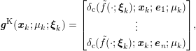 $$\begin{eqnarray}\boldsymbol{g}^{\text{K}}(\boldsymbol{x}_{k};\unicode[STIX]{x1D707}_{k};\boldsymbol{\unicode[STIX]{x1D709}}_{k})=\left[\begin{array}{@{}c@{}}\unicode[STIX]{x1D6FF}_{\text{c}}(\tilde{f}(\cdot ;\boldsymbol{\unicode[STIX]{x1D709}}_{k});\boldsymbol{x}_{k};\boldsymbol{e}_{1};\unicode[STIX]{x1D707}_{k})\\[2.0pt] \vdots \\[2.0pt] \unicode[STIX]{x1D6FF}_{\text{c}}(\tilde{f}(\cdot ;\boldsymbol{\unicode[STIX]{x1D709}}_{k});\boldsymbol{x}_{k};\boldsymbol{e}_{n};\unicode[STIX]{x1D707}_{k})\end{array}\right]\!,\end{eqnarray}$$
where
 $\unicode[STIX]{x1D6FF}_{\text{c}}(\cdot )$
is defined in (2.29)
The difference between (6.2) and (6.4) is analogous to the difference between one-point and two-point bandit feedback in the context of bandit problems (see Section 4.2). In the CRN regime, we can recall a single realization
 $\boldsymbol{\unicode[STIX]{x1D709}}_{k}$
to compute a finite-difference approximation in each coordinate direction. By using (6.4) as the gradient estimator in Algorithm 9, the rate (6.3) holds with
 $\unicode[STIX]{x1D6FE}=1/2$
(L’Ecuyer and Yin Reference L’Ecuyer and Yin1998, Kleinman, Spall and Naiman Reference Kleinman, Spall and Naiman1999). Thus, as in the analysis of bandit methods, the use of CRNs allows for strictly better convergence rate results.
Dai (Reference Dai and Dai2016a
, Reference Dai and Dai2016b
) studies the complexity of Algorithm 9, as well as a method that uses the estimator (6.2) in Algorithm 7, under varying assumptions on
 $\boldsymbol{\unicode[STIX]{x1D6EF}}$
. Dai considers a gradient estimate of the form (6.4) with
 $\unicode[STIX]{x1D6FF}_{\text{f}}(\tilde{f}(\cdot ;\boldsymbol{\unicode[STIX]{x1D709}}_{k});\boldsymbol{x}_{k};\boldsymbol{e}_{i};\unicode[STIX]{x1D707}_{k})$
replacing each central difference; recall the definition of
 $\unicode[STIX]{x1D6FF}_{\text{f}}(\cdot )$
in (2.28). Dai demonstrates that the best rate of the form (6.3) achievable by Algorithm 9with forward differences has
 $\unicode[STIX]{x1D6FE}=1/3$
, even when common random numbers are used. However, a rate of the form (6.3) with
 $\unicode[STIX]{x1D6FE}=1/2$
can be achieved using forward differences in Algorithm 7; Dai (Reference Dai and Dai2016a
, Reference Dai and Dai2016b
) draws parallels between this result and the WCC of Duchi et al. (Reference Duchi, Jordan, Wainwright and Wibisono2015), discussed in Section 4.2.2.
We remark that the gradient estimate (6.2) used in Algorithm 9requires
 $2n$
evaluations of
 $\tilde{f}$
per iteration. Although replacing
 $\unicode[STIX]{x1D6FF}_{\text{c}}(\tilde{f}(\cdot ;\boldsymbol{\unicode[STIX]{x1D709}}_{k});\boldsymbol{x}_{k};\boldsymbol{e}_{i};\unicode[STIX]{x1D707}_{k})$
with
 $\unicode[STIX]{x1D6FF}_{\text{f}}(\tilde{f}(\cdot ;\boldsymbol{\unicode[STIX]{x1D709}}_{k});\boldsymbol{x}_{k};\boldsymbol{e}_{i};\unicode[STIX]{x1D707}_{k})$
could reduce this cost to
 $n+1$
evaluations of
 $\tilde{f}$
per iteration, it is still desirable to reduce this per-iteration cost from
 $O(n)$
to
 $O(1)$
evaluations. The SPSA method of Spall (Reference Spall1992) achieves this goal by using the gradient estimator
 $$\begin{eqnarray}\boldsymbol{g}^{\text{S}}(\boldsymbol{x}_{k};\unicode[STIX]{x1D707}_{k};\boldsymbol{\unicode[STIX]{x1D709}}_{k};\boldsymbol{u}_{k})=\unicode[STIX]{x1D6FF}_{\text{c}}(\tilde{f}(\cdot ,\boldsymbol{\unicode[STIX]{x1D709}}_{k});\boldsymbol{x}_{k};\boldsymbol{u}_{k};\unicode[STIX]{x1D707}_{k})\left[\begin{array}{@{}c@{}}\displaystyle \frac{1}{[\boldsymbol{u}_{k}]_{1}}\\[2.0pt] \vdots \\[2.0pt] \displaystyle \frac{1}{[\boldsymbol{u}_{k}]_{n}}\end{array}\right]\!,\end{eqnarray}$$
where
 $\boldsymbol{u}_{k}\in \mathbb{R}^{n}$
is randomly generated from some distribution in each iteration.
The construction of (6.5) requires evaluations of
 $\tilde{f}(\cdot ;\boldsymbol{\unicode[STIX]{x1D709}}_{k})$
at exactly two points. Algorithm 9is then modified by replacing the gradient estimator
 $\boldsymbol{g}_{k}^{\text{K}}(\boldsymbol{x}_{k};\unicode[STIX]{x1D707}_{k};\boldsymbol{\unicode[STIX]{x1D709}}_{k})$
with
 $\boldsymbol{g}_{k}^{\text{S}}(\boldsymbol{x}_{k};\unicode[STIX]{x1D707}_{k};\boldsymbol{\unicode[STIX]{x1D709}}_{k};\boldsymbol{u}_{k})$
. Informally, the conditions on the distribution governing
 $\boldsymbol{u}_{k}$
originally proposed by Spall (Reference Spall1992) cause each entry of
 $\boldsymbol{u}_{k}$
to be bounded away from 0 with high probability (intuitively, to avoid taking huge steps). A simple example distribution satisfying these properties is to let each entry of
 $\boldsymbol{u}_{k}$
independently follow a Bernoulli distribution with support
 $\{1,-1\}$
, both events occurring with probability
 $1/2$
. Under appropriate assumptions resembling those for Algorithm 9, the sequence
 $\{\boldsymbol{x}_{k}\}$
generated by SPSA can be shown to converge in the same sense as Algorithm 9. Convergence rates of the form (6.3) matching those obtained for Algorithm 9have also been established (Gerencsér Reference Gerencsér1997, Kleinman et al.
Reference Kleinman, Spall and Naiman1999).
The performance of SA methods is highly sensitive to the chosen sequence of step sizes
 $\{\unicode[STIX]{x1D6FC}_{k}\}$
(Hutchison and Spall Reference Hutchison and Spall2013). This mirrors the situation in gradient-based SA methods where the tuning of algorithmic parameters is an active area of research (Diaz, Fokoue-Nkoutche, Nannicini and Samulowitz Reference Diaz, Fokoue-Nkoutche, Nannicini and Samulowitz2017, Ilievski, Akhtar, Feng and Shoemaker Reference Ilievski, Akhtar, Feng and Shoemaker2017, Balaprakash et al.
Reference Balaprakash, Salim, Uram, Vishwanath and Wild2018).
The SA methods above consider only a single evaluation of the stochastic function
 $\tilde{f}$
at any point. Other methods more accurately estimate
 $f(\boldsymbol{x}_{k})$
by querying
 $\tilde{f}(\boldsymbol{x}_{k};\boldsymbol{\unicode[STIX]{x1D709}})$
for multiple, different realizations (‘samples’) of
 $\boldsymbol{\unicode[STIX]{x1D709}}$
. These methods belong to the framework of sample average approximation, wherein the original problem (STOCH) is replaced with a (sequence of) deterministic sample-path problem(s):
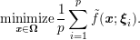
Retrospective approximation methods (Chen and Schmeiser Reference Chen and Schmeiser2001) vary the number of samples,
 $p$
, in a predetermined sequence
 $\{p_{0},p_{1},\ldots \}$
; the accuracy to which each instance of (6.6) subproblem is solved can also vary as a sample average approximation method progresses. Naturally, the performance of such a method depends critically on the sequence of sample sizes and accuracies used at each iteration; Pasupathy (Reference Pasupathy2010) characterizes a class of sequences of predetermined sample sizes and accuracies for which derivative-free retrospective approximation methods can be shown to converge for smooth objectives.
Other approaches dynamically adjust the number of samples
 $p$
from iteration to the next. For example, the method of Pasupathy, Glynn, Ghosh and Hashemi (Reference Pasupathy, Glynn, Ghosh and Hashemi2018) adjusts the number of samples
 $p_{k}$
to balance the contributions from deterministic and stochastic errors in iteration
 $k$
. The stochastic error at
 $\boldsymbol{x}_{k}$
is then
 $$\begin{eqnarray}\displaystyle \biggl|f(\boldsymbol{x}_{k})-\displaystyle \frac{1}{p_{k}}\mathop{\sum }_{i=1}^{p_{k}}\tilde{f}(\boldsymbol{x}_{k};\boldsymbol{\unicode[STIX]{x1D709}}_{k,i})\biggr|. & & \displaystyle \nonumber\end{eqnarray}$$
The deterministic error is the difference between the objective
 $f$
and a specified approximation; for example, the deterministic error at
 $\boldsymbol{x}_{k}-\unicode[STIX]{x1D6FC}_{k}\unicode[STIX]{x1D6FB}f(\boldsymbol{x}_{k})$
using a first-order Taylor approximation is
 $$\begin{eqnarray}\displaystyle |f(\boldsymbol{x}_{k}-\unicode[STIX]{x1D6FC}_{k}\unicode[STIX]{x1D6FB}f(\boldsymbol{x}_{k}))-(f(\boldsymbol{x}_{k})-\unicode[STIX]{x1D6FC}_{k}\Vert \unicode[STIX]{x1D6FB}f(\boldsymbol{x}_{k})\Vert ^{2})|. & & \displaystyle \nonumber\end{eqnarray}$$
Pasupathy et al. (Reference Pasupathy, Glynn, Ghosh and Hashemi2018) establish convergence rates for a variant of Algorithm 9drawing independent samples
 $\{\boldsymbol{\unicode[STIX]{x1D709}}_{k,1},\ldots ,\boldsymbol{\unicode[STIX]{x1D709}}_{k,p_{k}}\}$
in each iteration.
6.2 Direct-search methods for stochastic optimization
Unsurprisingly, researchers have modified methods for deterministic objectives in order to produce methods appropriate for stochastic optimization. For example, in the paper inspiring Nelder and Mead (Reference Nelder and Mead1965), Spendley et al. (Reference Spendley, Hext and Himsworth1962) propose re-evaluating the point corresponding to the best simplex vertex if it hasn’t changed in
 $n+1$
iterations, saying that if the vertex is best ‘only by reason of errors of observation, it is unlikely that the repeat observation will [be the best observed point], and the point will be eliminated in due course’. Barton and Ivey, Jr (Reference Barton and Ivey1996) propose modifications to the Nelder–Mead method in order to avoid premature termination due to repeated shrinking. To alleviate this problem, they suggest reducing the amount the simplex is shrunk, re-evaluating the best point after each shrink operation, and re-evaluating each reflected point before performing a contraction. Chang (Reference Chang2012) proposes a Nelder–Mead variant that samples candidate points and all other points in the simplex an increasing number of times; this method ultimately ensures that stochasticity in the function evaluations will not affect the correct ranking of simplex vertices.
Sriver, Chrissis and Abramson (Reference Sriver, Chrissis and Abramson2009) augment a GPS method with a ranking and selection procedure and dynamically determine the number of samples performed for each polling point. The ranking and selection procedure allows the method to also address cases where
 $\boldsymbol{x}$
contains discrete variables. For the case of additive unbiased, Gaussian noise (i.e.
 $\tilde{f}(\boldsymbol{x};\boldsymbol{\unicode[STIX]{x1D709}})=f(\boldsymbol{x})+\unicode[STIX]{x1D70E}\boldsymbol{\unicode[STIX]{x1D709}}$
with
 $\boldsymbol{\unicode[STIX]{x1D709}}$
from a standard normal distribution and
 $\unicode[STIX]{x1D70E}>0$
finite), they prove that the resulting method converges almost surely to a stationary point of
 $f$
. For problems involving more general distributions, Kim and Zhang (Reference Kim and Zhang2010) consider a DDS method that employs the sample mean
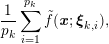 $$\begin{eqnarray}\displaystyle \frac{1}{p_{k}}\mathop{\sum }_{i=1}^{p_{k}}\tilde{f}(\boldsymbol{x};\boldsymbol{\unicode[STIX]{x1D709}}_{k,i}),\end{eqnarray}$$
with a dynamically increasing sample size
 $p_{k}$
. They establish a consistency result and appeal to the convergence properties of DDS methods. Sankaran, Audet and Marsden (Reference Sankaran, Audet and Marsden2010) propose a surrogate-assisted method for stochastic optimization inspired by stochastic collocation techniques (see e.g. Gunzburger, Webster and Zhang Reference Gunzburger, Webster and Zhang2014). Convergence for the method is established by appealing to the GPS and MADS mechanisms underlying the method.
Chen and Kelley (Reference Chen and Kelley2016) consider an implicit-filtering method in which values of
 $f$
are observable only through the sample average (6.7). Chen and Kelley (Reference Chen and Kelley2016) demonstrate that the sequence of points generated by the method converges (i.e.
 $\{\unicode[STIX]{x1D6FB}f(\boldsymbol{x}_{k})\}$
admits a subsequence that converges to zero) with probability one if the sample size
 $p_{k}$
increases to infinity. Algorithmically,
 $p_{k}$
is adjusted to scale with the square of the inverse of the stencil step size (
 $\unicode[STIX]{x1D6E5}_{k}$
in Algorithm 4).
Chen, Kelley, Xu and Zhang (Reference Chen, Kelley, Xu and Zhang2018b
) consider the bound-constrained minimization of a composite non-smooth function of the form (5.5), where
 $h$
is Lipschitz-continuous (but non-smooth) and
 $\boldsymbol{F}$
is continuously differentiable. However, they assume that values of
 $\boldsymbol{F}$
are observable only through sample averages and that a smoothing function
 $h_{\unicode[STIX]{x1D707}}$
of
 $h$
(as discussed in Section 5.3.2) is available. They show that with probability one, the sequence of points from a smoothed implicit-filtering method converges to a first-order stationary point, where the stationarity measure is appropriate for non-smooth optimization.
6.3 Model-based methods for stochastic optimization
Analysis of the model-based trust-region methods in Section 2.2 generally depends on the construction of fully linear models of a deterministic function
 $f$
; see (2.9). In particular, methods of the form of Algorithm 3typically require that a model
 $m_{k}$
satisfy
 $$\begin{eqnarray}\displaystyle |f(\boldsymbol{x}_{k}+\boldsymbol{s})-m_{k}(\boldsymbol{x}_{k}+\boldsymbol{s})|\leq \unicode[STIX]{x1D705}_{\text{ef}}\unicode[STIX]{x1D6E5}_{k}^{2}\quad \text{for all}~\boldsymbol{s}\in {\mathcal{B}}(\mathbf{0};\unicode[STIX]{x1D6E5}_{k}). & & \displaystyle \nonumber\end{eqnarray}$$
A natural model-based trust-region approach to stochastic optimization is to build a model
 $m_{k}$
of the function
 $f$
by fitting the model to observed values of the stochastic function
 $\tilde{f}$
. Intuitively, if such models satisfy (2.9), then an extension of the analysis described in Section 2.2.4 should also apply to the minimization of
 $f$
in (STOCH). The methods described here formalize the approximation properties of such models (which are stochastic because of their dependence on
 $\boldsymbol{\unicode[STIX]{x1D709}}$
) and employ the models in a trust-region framework. For example, by employing an estimator
 $\bar{f}_{p}$
of
 $f$
at each interpolation point
 $\boldsymbol{x}$
used in model construction, we can replace each function value
 $f(\boldsymbol{x})$
with
 $\bar{f}_{p}(\boldsymbol{x})$
in the interpolation system (2.14). One example of such an estimator
 $\bar{f}_{p}$
is the sample average (6.7).
Early work in applying derivative-free trust-region methods for stochastic optimization includes that of Deng and Ferris (Reference Deng and Ferris2006), which modifies the UOBYQA method of Powell (Reference Powell2002). The
 $k$
th iteration of the method of Deng and Ferris (Reference Deng and Ferris2006) uses Bayesian techniques to dynamically update a budget of
 $p_{k}$
new
 $\tilde{f}$
evaluations. This budget is then apportioned among the current set of interpolation points
 $\boldsymbol{y}\in \boldsymbol{Y}$
in order to reduce the variance in each value of
 $\bar{f}_{p_{k}}(\boldsymbol{y})$
, with the authors using the sample mean for the estimator
 $\bar{f}_{p_{k}}$
. Deng and Ferris (Reference Deng and Ferris2009) show that, given assumptions on the sequence of evaluated
 $\boldsymbol{\unicode[STIX]{x1D709}}$
(i.e. the sample path), every limit point
 $\boldsymbol{x}_{\ast }$
produced by this method is stationary with probability 1.
Another method in this vein, STRONG, was proposed by Chang, Hong and Wan (Reference Chang, Hong and Wan2013) and combines response surface methodology (Box and Draper Reference Box and Draper1987) with a trust-region mechanism. In the analysis of STRONG, it is assumed that model gradients
 $\unicode[STIX]{x1D6FB}m_{k}(\boldsymbol{x}_{k})$
almost surely equal the true gradients
 $\unicode[STIX]{x1D6FB}f(\boldsymbol{x}_{k})$
as
 $k\rightarrow \infty$
, which is algorithmically encouraged by monotonically increasing the sample size
 $p_{k}$
in an inner loop. QNSTOP by Castle (Reference Castle2012) presents a similar approach using response surface models in a trust-region framework, but its convergence analysis and assumptions mirror those of stochastic approximation methods.
Both Larson and Billups (Reference Larson and Billups2016) and Chen, Menickelly and Scheinberg (Reference Chen, Menickelly and Scheinberg2018a
) build on the idea of probabilistically fully linear models in (3.5), which essentially says that the condition (2.9) needs to hold on a given iteration only with some probability (Bandeira et al.
Reference Bandeira, Scheinberg and Vicente2014). In contrast to the usage of such models in randomized methods for deterministic objectives (the subject of Section 3.3), in stochastic optimization the filtration in (3.5) also includes the realizations of the stochastic evaluations of
 $\tilde{f}$
. This probabilistic notion of uniform local model quality is powerful. For example, although the connection is not made by Regier, Jordan and McAuliffe (Reference Regier, Jordan, McAuliffe and Guyon2017), this notion of model quality implies probabilistic descent properties such as those required by Regier et al. (Reference Regier, Jordan, McAuliffe and Guyon2017). This implication is an example of a setting in which stochastic gradient estimators can be replaced by gradients of probabilistically fully linear models.
One way to satisfy (3.5) is to build a regression model using randomly sampled points. For example, Menickelly (Reference Menickelly2017, Theorem 4.2.6) shows that evaluating
 $\tilde{f}$
on a sufficiently large set of points uniformly sampled from
 ${\mathcal{B}}(\boldsymbol{x}_{k};\unicode[STIX]{x1D6E5}_{k})$
can be used to construct a probabilistically fully linear regression model.
Larson and Billups (Reference Larson and Billups2016) prove convergence of a probabilistic variant of Algorithm 3in the sense that, for any
 $\unicode[STIX]{x1D716}>0$
,
 $$\begin{eqnarray}\displaystyle \lim _{k\rightarrow \infty }\mathbb{P}[\Vert \unicode[STIX]{x1D6FB}f(\boldsymbol{x}_{k})\Vert >\unicode[STIX]{x1D716}]=0. & & \displaystyle \nonumber\end{eqnarray}$$
Under similar assumptions, Chen et al. (Reference Chen, Menickelly and Scheinberg2018a ) prove almost sure convergence to a stationary point, that is,
 $$\begin{eqnarray}\lim _{k\rightarrow \infty }\Vert \unicode[STIX]{x1D6FB}f(\boldsymbol{x}_{k})\Vert =0\quad \text{with probability one}.\end{eqnarray}$$
Blanchet, Cartis, Menickelly and Scheinberg (Reference Blanchet, Cartis, Menickelly and Scheinberg2019) provide a WCC result for the variant of Algorithm 3presented by Chen et al. (Reference Chen, Menickelly and Scheinberg2018a
). Blanchet et al. (Reference Blanchet, Cartis, Menickelly and Scheinberg2019) extend the analysis of Cartis and Scheinberg (Reference Cartis and Scheinberg2018) to study the stopping time of the stochastic process generated by the method of Chen et al. (Reference Chen, Menickelly and Scheinberg2018a
). In contrast to previous WCC results discussed in this survey, which bound the number of function evaluations
 $N_{\unicode[STIX]{x1D716}}$
needed to attain some form of expected
 $\unicode[STIX]{x1D716}$
-optimality (e.g. (3.2) or (5.4)), Blanchet et al. (Reference Blanchet, Cartis, Menickelly and Scheinberg2019) prove that the expected number of iterations,
 $\mathbb{E}[T_{\unicode[STIX]{x1D716}}]$
, needed to achieve (2.2) is in
 $O(\unicode[STIX]{x1D716}^{-2})$
. Paquette and Scheinberg (Reference Paquette and Scheinberg2018) apply similar analysis to a derivative-free stochastic line-search method, where they demonstrate that for non-convex
 $f$
,
 $\mathbb{E}[T_{\unicode[STIX]{x1D716}}]\in O(\unicode[STIX]{x1D716}^{-2})$
, while for convex and strongly convex
 $f$
,
 $\mathbb{E}[T_{\unicode[STIX]{x1D716}}]\in O(\unicode[STIX]{x1D716}^{-1})$
and
 $\mathbb{E}[T_{\unicode[STIX]{x1D716}}]\in O(\log (\unicode[STIX]{x1D716}^{-1}))$
, respectively. Since the number of function evaluations per iteration of the derivative-free methods of Blanchet et al. (Reference Blanchet, Cartis, Menickelly and Scheinberg2019) and Paquette and Scheinberg (Reference Paquette and Scheinberg2018) is highly variable across iterations, the total work (in terms of function evaluations) is not readily apparent from such WCC results.
Larson and Billups (Reference Larson and Billups2016) and Chen et al. (Reference Chen, Menickelly and Scheinberg2018a
) demonstrate that sampling
 $\tilde{f}$
on
 ${\mathcal{B}}(\boldsymbol{x}_{k};\unicode[STIX]{x1D6E5}_{k})$
of the order of
 $\unicode[STIX]{x1D6E5}_{k}^{-4}$
times will ensure that (2.9) holds (i.e. one can obtain a fully linear model) with high probability. Shashaani, Hunter and Pasupathy (Reference Shashaani, Hunter and Pasupathy2016) and Shashaani, Hashemi and Pasupathy (Reference Shashaani, Hashemi and Pasupathy2018) take a related but distinct approach. As opposed to requiring that models be probabilistically fully linear, their derivative-free trust-region method performs adaptive Monte Carlo sampling both at current points
 $\boldsymbol{x}_{k}$
and interpolation points; the number of samples
 $p_{k}$
is chosen to balance a measure of statistical error with the optimality gap at
 $\boldsymbol{x}_{k}$
. Shashaani et al. (Reference Shashaani, Hashemi and Pasupathy2018) prove that their method achieves almost sure convergence of the form (6.8).
A model-based trust-region method for constrained stochastic optimization, SNOWPAC, is developed by Augustin and Marzouk (Reference Augustin and Marzouk2017). Their method addresses the stochasticity by employing Gaussian process-based models of robustness measures such as expectation and conditional value at risk. The approach used is an extension of the constrained deterministic method NOWPAC of Augustin and Marzouk (Reference Augustin and Marzouk2014), which we discuss in Section 7.
6.4 Bandit feedback methods
While much of the literature on bandit methods for stochastic optimization focuses on convex objectives
 $f$
(as discussed in Section 4.2), here we discuss treatment of non-convex objectives
 $f$
. We recall our notation and discussion from Section 4.2, in particular the notion of regret minimization shown in (4.7).
In the absence of convexity, regret bounds do not translate into bounds on optimization error as easily as in (4.8). Some works address the case where each
 $\tilde{f}(\cdot ;\boldsymbol{\unicode[STIX]{x1D709}}_{k})$
in (4.7) is Lipschitz-continuous and employ a partitioning of the feasible region
 $\boldsymbol{\unicode[STIX]{x1D6FA}}$
(Kleinberg, Slivkins and Upfal Reference Kleinberg, Slivkins and Upfal2008, Bubeck, Stoltz and Yu Reference Bubeck, Stoltz, Yu and Kivinen2011b
, Bubeck, Munos, Stoltz and Szepesvári Reference Bubeck, Munos, Stoltz and Szepesvári2011a
, Valko, Carpentier and Munos Reference Valko, Carpentier and Munos2013, Zhang, Yang, Jin and Zhou Reference Zhang, Yang, Jin and Zhou2015). These methods employ global optimization strategies that we do not discuss further here.
In another line of work, Ghadimi and Lan (Reference Ghadimi and Lan2013) consider the application of an algorithm like Algorithm 6with the choice of gradient estimator
 $\boldsymbol{g}_{\unicode[STIX]{x1D707}}(\boldsymbol{x};\boldsymbol{u};\boldsymbol{\unicode[STIX]{x1D709}})$
from (4.12). Under an assumption of bounded variance of the estimator (i.e.
 $\mathbb{E}_{\boldsymbol{\unicode[STIX]{x1D709}}}[\Vert \boldsymbol{g}_{\unicode[STIX]{x1D707}}(\boldsymbol{x};\boldsymbol{u};\boldsymbol{\unicode[STIX]{x1D709}})-\unicode[STIX]{x1D6FB}f(\boldsymbol{x})\Vert ^{2}]\leq \unicode[STIX]{x1D70E}^{2}$
), Ghadimi and Lan (Reference Ghadimi and Lan2013) prove a WCC result similar to the one they obtained in the convex case; see Section 4.2.2. They show that an upper bound on the (randomized) number of iterations needed to attain
 $$\begin{eqnarray}\mathbb{E}_{}[\Vert \unicode[STIX]{x1D6FB}f(\boldsymbol{x}_{k})\Vert ^{2}]\leq \unicode[STIX]{x1D716}\end{eqnarray}$$
is in
 $O(\max \{nL_{g}R_{\boldsymbol{x}}\unicode[STIX]{x1D716}^{-1},nL_{g}R_{\boldsymbol{x}}\unicode[STIX]{x1D70E}^{2}\unicode[STIX]{x1D716}^{-2}\})$
. Notice that the stationarity condition given in (6.9) involves a square on the gradient norm, making it distinct from a result like (3.2) or (5.4). Thus, assuming
 $\unicode[STIX]{x1D70E}^{2}$
is sufficiently large, the result of Ghadimi and Lan (Reference Ghadimi and Lan2013) translates to a WCC of type (5.4) in
 $O(n^{2}\unicode[STIX]{x1D716}^{-4})$
.
Balasubramanian and Ghadimi (Reference Balasubramanian, Ghadimi and Bengio2018, Reference Balasubramanian and Ghadimi2019) propose a method that uses two-point bandit feedback (i.e. a gradient estimator from (4.12)) within a derivative-free conditional gradient method (Ghadimi Reference Ghadimi2019). The gradient estimator is used to define a linear model, which is minimized over
 $\boldsymbol{\unicode[STIX]{x1D6FA}}$
to produce a trial step. If
 $\boldsymbol{\unicode[STIX]{x1D6FA}}$
is bounded, they show a WCC of type (5.4) that again grows like
 $\unicode[STIX]{x1D716}^{-4}$
.
By replacing gradients with estimators of the form (4.12) in the stochastic variance-reduced gradient framework of machine learning (Reddi et al.
Reference Reddi, Hefny, Sra, Poczos, Smola, Balcan and Weinberger2016), Liu et al. (Reference Liu, Kailkhura, Chen, Ting, Chang, Amini and Bengio2018) prove a WCC of type (6.9) in
 $O(n\unicode[STIX]{x1D716}^{-1}+b^{-1})$
, where
 $b$
is the size of a minibatch drawn with replacement in each iteration. Gu, Huo and Huang (Reference Gu, Huo and Huang2016) prove a similar WCC result in an asynchronous parallel computing environment for a distinct method using minibatches for variance reduction.
7 Methods for constrained optimization
In this section, we discuss derivative-free methods for problems where the feasible region
 $\boldsymbol{\unicode[STIX]{x1D6FA}}$
is a proper subset of
 $\mathbb{R}^{n}$
. In the derivative-free setting, such constrained optimization problems can take many forms since an additional distinction is associated with the derivative-free nature of objective and constraint functions. For example, and in contrast to the preceding sections, a derivative-free constrained optimization problem may involve an objective function
 $f$
for which a gradient is made available to the optimization method. The problem is still derivative-free if there is a constraint function defining the feasible region
 $\boldsymbol{\unicode[STIX]{x1D6FA}}$
for which a (sub)gradient is not available to the optimization method.
As is common in many application domains where derivative-free methods are applied, the feasible region
 $\boldsymbol{\unicode[STIX]{x1D6FA}}$
may also involve discrete choices. In particular, these choices can include categorical variables that are either ordinal (e.g. letter grades in
 $\{$
A, B, C, D, F
 $\}$
) or non-ordinal (e.g. compiler type in
 $\{$
flang, gfortran, ifort
 $\}$
). Although ordinal categorical variables can be mapped to a subset of the reals, the same cannot be done for non-ordinal variables. Therefore, we generalize the formulations of (DET) and (STOCH) to the problem

where
 $\boldsymbol{y}$
represents a vector of non-ordinal variables and
 $\mathbf{N}$
is a finite set of feasible values. Here we assume that discrete-valued ordinal variables are included in
 $\boldsymbol{x}$
. Furthermore, most of the methods we discuss do not explicitly treat non-ordinal variables
 $\boldsymbol{y}$
; hence, except where indicated, we will drop the use of
 $\boldsymbol{y}$
.
Similar to Section 5, here we distinguish methods based on the assumptions made about the problem structure. We organize these assumptions based on the black-box optimization constraint taxonomy of Le Digabel and Wild (Reference Le Digabel and Wild2015), which characterizes the type of constraint functions that occur in a particular specification of a derivative-free optimization problem. When constraints are explicitly stated (i.e. ‘known’ to the method), this taxonomy takes the form of the tree in Figure 7.1.
Tree-based taxonomy of known (i.e. non-hidden) constraints from Le Digabel and Wild (2015).
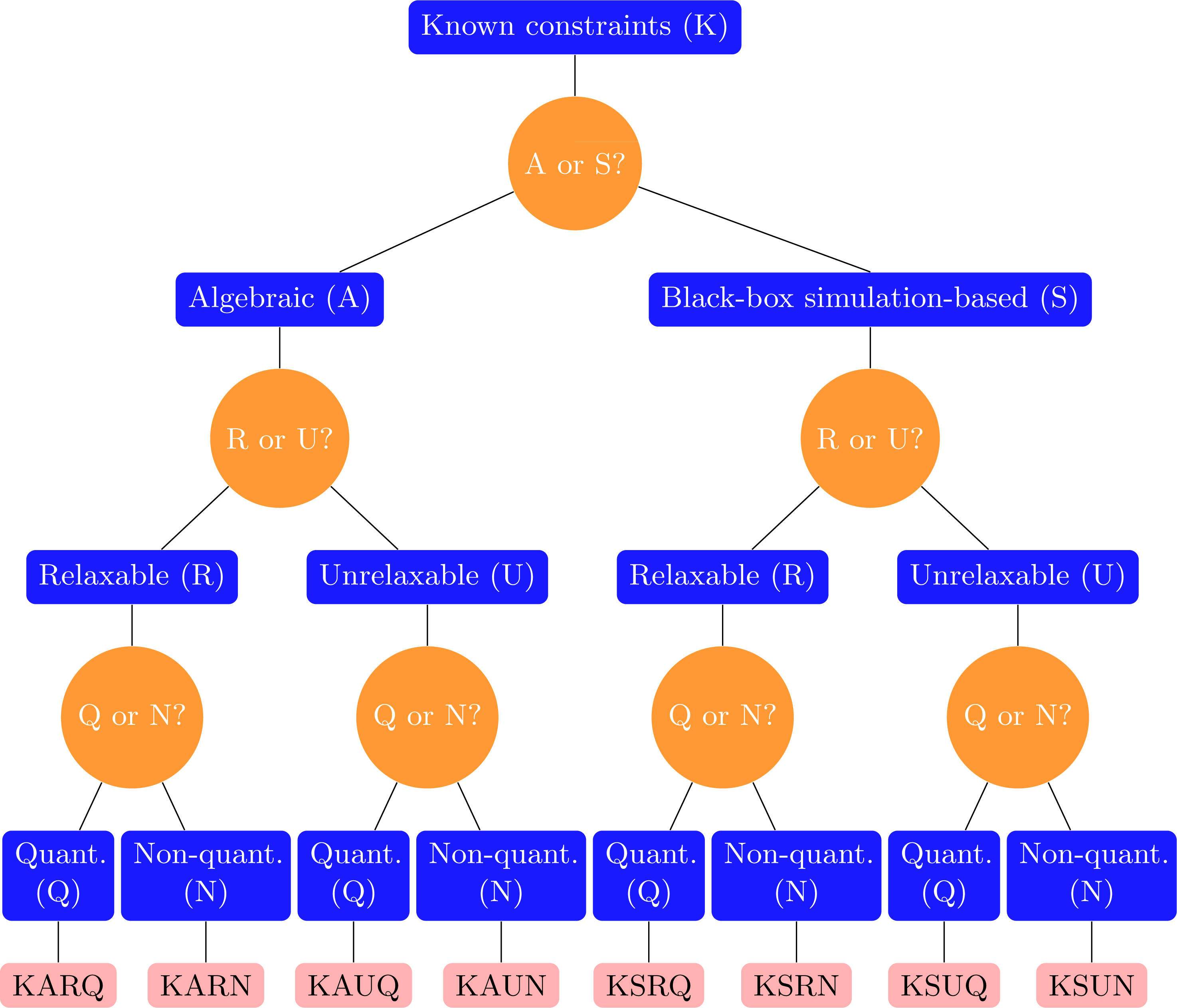
The first distinction in Figure 7.1 is whether a constraint is algebraically available to the optimization method or whether it depends on a black-box simulation. In the context of derivative-free optimization, we will assume that it is these latter constraint functions for which a (sub)gradient is not made available to the optimization method. Algebraic constraints are those for which a functional form or simple projection operator is provided to the optimization method. Section 7.1 discusses methods that exclusively handle algebraic constraints. Examples of such algebraic constraints have been discussed earlier in this paper (e.g. Sections 3.1 and 4), wherein it is assumed that satisfaction of the constraints (e.g. through a simple projection) is trivial relative to evaluation of the objective. This imbalance between the ease of the constraint and objective functions is also the subject of recent WCC analysis (Cartis, Gould and Toint Reference Cartis, Gould and Toint2018).
Section 7.2 discusses methods that target situations where one or more constraints do not have available derivatives.
The next distinction in Figure 7.1 is whether a constraint can be relaxed or whether the constraint must be satisfied in order to obtain meaningful information for the objective
 $f$
and/or other constraint functions. Unrelaxable constraints are a relatively common occurrence in derivative-free optimization. In contrast to classic optimization, constraints are sometimes introduced solely to prevent errors in the evaluation of, for example, a simulation-based objective function. Methods for addressing relaxable algebraic constraints are discussed in Section 7.1.1, and unrelaxable algebraic constraints are the focus of Section 7.1.2.
Hidden constraints are not represented in Figure 7.1. Hidden constraints are constraints that are not explicitly stated in a problem specification. Violating these constraints is detected only when attempting to evaluate the objective or constraint functions; for example, a simulation may fail to return output, thus leaving one of these functions undefined. Some derivative-free methods directly account for the possibility that such failures may be present despite not being explicitly stated. Hidden constraints have been addressed in works including those of Avriel and Wilde (Reference Avriel and Wilde1967), Choi and Kelley (Reference Choi and Kelley2000), Choi et al. (Reference Choi, Eslinger, Kelley, David and Etheridge2000), Carter et al. (Reference Carter, Gablonsky, Patrick, Kelley and Eslinger2001), Conn, Scheinberg and Toint (Reference Conn, Scheinberg and Toint2001), Huyer and Neumaier (Reference Huyer and Neumaier2008), Lee, Gramacy, Linkletter and Gray (Reference Lee, Gramacy, Linkletter and Gray2011), Chen and Kelley (Reference Chen and Kelley2016), Porcelli and Toint (Reference Porcelli and Toint2017) and Müller and Day (Reference Müller and Day2019).
7.1 Algebraic constraints
When all constraints are algebraically available, we can characterize the ordinal feasible region by a collection of inequality constraints:
 $$\begin{eqnarray}\boldsymbol{\unicode[STIX]{x1D6FA}}=\{\boldsymbol{x}\in \mathbb{R}^{n}:c_{i}(\boldsymbol{x})\leq 0,\text{ for all }i\in I\},\end{eqnarray}$$
where each
 $c_{i}:\mathbb{R}^{n}\rightarrow \mathbb{R}\cup \{\infty \}$
and the set
 $I$
is finite for all of the methods discussed. Problems with semi-infinite constraints can be addressed by using structured approaches as in Section 5.4. In this setting, we define the constraint function
 $\boldsymbol{c}~:~\mathbb{R}^{n}\rightarrow (\mathbb{R}\cup \{\infty \})^{|I|}$
, where the
 $i$
th entry of the vector
 $\boldsymbol{c}(\boldsymbol{x})$
is given by
 $c_{i}(\boldsymbol{x})$
. Equality constraints can be represented in (7.1) by including both
 $c_{i}(\boldsymbol{x})$
and
 $-c_{i}(\boldsymbol{x})$
; however, this practice should be avoided since it can hamper both theoretical and empirical performance.
7.1.1 Relaxable algebraic constraints
Relaxable algebraic constraints are the constraints that are typically treated in derivative-based non-linear optimization. We will organize our discussion into three primary types of methods: penalty approaches, filter approaches, and approaches with subproblems that employ models of the constraint functions.
Penalty approaches.
Given constraints defined by (7.1), it is natural in the setting of relaxable constraints to quantify the violation of the
 $i$
th constraint via the value of
 $\max \{0,c_{i}(\boldsymbol{x})\}$
. In fact, given a penalty parameter
 $\unicode[STIX]{x1D70C}>0$
, a common approach in relaxable constrained optimization is to replace the minimization of
 $f(\boldsymbol{x})$
with the minimization of a merit function such as
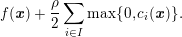 $$\begin{eqnarray}f(\boldsymbol{x})+\displaystyle \frac{\unicode[STIX]{x1D70C}}{2}\displaystyle \mathop{\sum }_{i\in I}\max \{0,c_{i}(\boldsymbol{x})\}.\end{eqnarray}$$
The merit function in (7.2) is typically called an exact penalty function, because for a sufficiently large (but finite) value of
 $\unicode[STIX]{x1D70C}>0$
, every local minimum
 $\boldsymbol{x}_{\ast }$
of (CON) is also a local minimum of the merit function in (7.2). We note that each summand
 $\max \{0,c_{i}(\boldsymbol{x})\}$
is generally non-smooth; the summand is still convex provided
 $c_{i}(\boldsymbol{x})$
is convex. Through the mapping
 $$\begin{eqnarray}\boldsymbol{F}(\boldsymbol{x})=\left[\begin{array}{@{}c@{}}f(\boldsymbol{x})\\ \boldsymbol{ c}(\boldsymbol{x})\end{array}\right]\!,\end{eqnarray}$$
functions of the form (7.2) can be seen as cases of the composite non-smooth function (5.5) and are hence amenable to the methods discussed in Section 5.3. In contrast to this non-smooth approach, a more popular merit function historically has been the quadratic penalty function,
 $$\begin{eqnarray}f(\boldsymbol{x})+\unicode[STIX]{x1D70C}\displaystyle \mathop{\sum }_{i\in I}\max \{0,c_{i}(\boldsymbol{x})\}^{2}.\end{eqnarray}$$
However, the merit function in (7.3) lacks the same exactness guarantees that come with (7.2); even as
 $\unicode[STIX]{x1D70C}$
grows arbitrarily large, local minima of (CON) need not correspond in any way with minima of (7.3).
Another popular means of maintaining the smoothness (and convexity, when applicable) of (7.3) but regaining the exactness of (7.2) is to consider Lagrangian-based merit functions. Associating multipliers
 $\unicode[STIX]{x1D706}_{i}$
with each of the constraints in (7.1), the Lagrangian of (CON) is
 $$\begin{eqnarray}L(\boldsymbol{x};\boldsymbol{\unicode[STIX]{x1D706}})=f(\boldsymbol{x})+\mathop{\sum }_{i\in I}\unicode[STIX]{x1D706}_{i}\,c_{i}(\boldsymbol{x}).\end{eqnarray}$$
Combining (7.4) with (7.3) yields the augmented Lagrangian merit function
 $$\begin{eqnarray}L_{A}(\boldsymbol{x};\boldsymbol{\unicode[STIX]{x1D706}};\unicode[STIX]{x1D70C})=f(\boldsymbol{x})+\mathop{\sum }_{i\in I}\unicode[STIX]{x1D706}_{i}\,c_{i}(\boldsymbol{x})+\displaystyle \frac{\unicode[STIX]{x1D70C}}{2}\mathop{\sum }_{i\in I}\max \{0,c_{i}(\boldsymbol{x})\}^{2}\end{eqnarray}$$
with the desired properties; that is, for non-negative
 $\boldsymbol{\unicode[STIX]{x1D706}}$
and
 $\unicode[STIX]{x1D70C}$
,
 $L_{A}(\boldsymbol{x};\boldsymbol{\unicode[STIX]{x1D706}};\unicode[STIX]{x1D70C})$
is smooth (convex) provided that
 $\boldsymbol{c}$
is.
In all varieties of these methods, which we broadly refer to as penalty approaches, the parameter
 $\unicode[STIX]{x1D70C}$
is dynamically updated between iterations. Methods typically increase
 $\unicode[STIX]{x1D70C}$
in order to promote feasibility; penalty methods tend to approach solutions from outside of
 $\boldsymbol{\unicode[STIX]{x1D6FA}}$
and hence typically assume that the penalized constraints are relaxable. For a review of general penalty approaches, see Fletcher (Reference Fletcher1987, Chapter 12).
Lewis and Torczon (Reference Lewis and Torczon2002) adapt the augmented Lagrangian approach of Conn, Gould and Toint (Reference Conn, Gould and Toint1991) in one of the first proofs that DDS methods can be globally convergent for non-linear optimization. They utilize pattern search (see the discussion in Section 2.1.2) to approximately minimize the augmented Lagrangian function (7.5) in each iteration of their method. That is, each iteration of their method solves a subproblem

Lewis and Torczon (Reference Lewis and Torczon2002) prove global convergence of their method to first-order Karush–Kuhn–Tucker (KKT) points. We note that the algebraic availability of bound constraints is explicitly used in (7.6). Other constraints could be algebraic or simulation-based because the method used to approximately solve (7.6) does not require availability of the derivative
 $\unicode[STIX]{x1D6FB}_{\boldsymbol{x}}L_{A}(\boldsymbol{x};\boldsymbol{\unicode[STIX]{x1D706}};\unicode[STIX]{x1D70C})$
. The approach of Lewis and Torczon (Reference Lewis and Torczon2002) is expanded by Lewis and Torczon (Reference Lewis and Torczon2010), who demonstrate the benefits of treating linear constraints (including bound constraints) outside of the augmented Lagrangian merit function. That is, they consider subproblems of the form

Bueno, Friedlander, Martínez and Sobral (Reference Bueno, Friedlander, Martínez and Sobral2013) propose an inexact restoration method for problems (CON) where
 $\boldsymbol{\unicode[STIX]{x1D6FA}}$
is given by equality constraints. The inexact restoration method alternates between improving feasibility (measured through the constraint violation
 $\Vert \boldsymbol{c}(\boldsymbol{x})\Vert _{2}$
in this equality-constrained case) and then approximately minimizing a
 $\Vert \cdot \Vert _{2}$
-based exact penalty function before dynamically adjusting the penalty parameter
 $\unicode[STIX]{x1D70C}$
. Because of the separation of the feasibility and optimality phases of the inexact restoration method, the feasibility phase requires no evaluations of
 $f$
. This feasibility phase is easier when constraint functions are available algebraically because (sub)derivative-based methods can be employed. Bueno et al. (Reference Bueno, Friedlander, Martínez and Sobral2013) prove global convergence to first-order KKT points of this method under appropriate assumptions.
Amaioua, Audet, Conn and Le Digabel (Reference Amaioua, Audet, Conn and Le Digabel2018) study the performance of a search step in MADS when solving (CON). One of their approaches uses the exact penalty (7.2), a second approach uses the augmented Lagrangian (7.5) and a third combines these two.
Audet, Le Digabel and Peyrega (Reference Audet, Le Digabel and Peyrega2015) show that the convergence properties of MADS extend to problems with linear equality constraints. They explicitly address these algebraic constraints by reformulating the original problem into a new problem without equality constraints (and possibly fewer variables); other constraints are treated as will be discussed in Section 7.2.
Filter approaches.
Whereas a penalty approach combines an objective function
 $f$
and a measure of constraint violation into a single merit function to be minimized approximately, a filter method can be understood as a biobjective method minimizing the objective and the constraint violation simultaneously. For this general discussion, we will refer to the measure of constraint violation as
 $h(\boldsymbol{x})$
. For example, in (7.2),
 $$\begin{eqnarray}\displaystyle h(\boldsymbol{x})=\displaystyle \mathop{\sum }_{i\in I}\max \{0,c_{i}(\boldsymbol{x})\}. & & \displaystyle \nonumber\end{eqnarray}$$
From the perspective of biobjective optimization, a filter can be understood as a subset of non-dominated points in the (
 $f,h$
) space. A two-dimensional point
 $(f(\boldsymbol{x}_{l}),h(\boldsymbol{x}_{l}))$
is non-dominated, in the finite set of points
 $\{\boldsymbol{x}_{j}:j\in J\}$
evaluated by a method, provided there is no
 $j\in J\setminus \{l\}$
with
 $$\begin{eqnarray}\displaystyle f(\boldsymbol{x}_{j})\leq f(\boldsymbol{x}_{l})\quad \text{and}\quad h(\boldsymbol{x}_{j})\leq h(\boldsymbol{x}_{l}). & & \displaystyle \nonumber\end{eqnarray}$$
Unlike biobjective optimization, however, filter methods adaptively vary the subset of non-dominated points considered in order to identify feasible points (i.e. points where
 $h$
vanishes). Different filter methods employ different mechanisms for managing the filter and generating new points.
Brekelmans, Driessen, Hamers and den Hertog (Reference Brekelmans, Driessen, Hamers and den Hertog2005) employ a filter for handling relaxable algebraic constraints. Their model-based method attempts to have model-improving points satisfy the constraints. Ferreira, Karas, Sachine and Sobral (Reference Ferreira, Karas, Sachine and Sobral2017) extend the inexact-restoration method of Bueno et al. (Reference Bueno, Friedlander, Martínez and Sobral2013) by replacing the penalty formulation with a filter mechanism and again prove global convergence to first-order KKT points.
Approaches with subproblems using modelled constraints.
Another means of constraint handling is to construct local models
 $m^{c_{i}}$
of each constraint
 $c_{i}$
in (7.1). Given a local model
 $m^{f}$
of the objective function
 $f$
, such methods generally employ a sequence of subproblems of the form

As an example approach, sequential quadratic programming (SQP) methods are popular derivative-based methods that employ a quadratic model of the objective function and linear models of the constraint functions. Several derivative-free approaches of this form exist, which we detail in this section. We mention that many of these approaches will generally impose an additional trust-region constraint (i.e.
 $\Vert \boldsymbol{s}\Vert \leq \unicode[STIX]{x1D6E5}$
) on (7.8). As in Section 2.2.4, this trust-region constraint often has the additional role of monitoring the quality of the model
 $m^{f}$
. Furthermore, such a trust-region constraint ensures that whenever
 $\boldsymbol{s}=\mathbf{0}$
is feasible for (7.8), the feasible region of (7.8) is compact.
Conn, Scheinberg and Toint (Reference Conn, Scheinberg and Toint1998) consider an adaptation of a model-based trust-region method to constrained problems with differentiable algebraic constraints treated via the trust-region subproblem (7.8). They target problems where they deem the algebraic constraints to be ‘easy’, meaning that the resulting trust-region subproblem is not too difficult to solve. This method is implemented in the solver DFO (Conn et al. Reference Conn, Scheinberg and Toint2001).
The CONDOR method of Vanden Berghen (Reference Vanden Berghen2004) and Vanden Berghen and Bersini (Reference Vanden Berghen and Bersini2005) extends the unconstrained UOBYQA method of Powell (Reference Powell2002) to address algebraic constraints. The trust-region subproblem considered takes the form

where
 $m^{f}$
is a quadratic model and
 $I^{\prime }\subseteq I$
captures the non-linear constraints in (7.1). In solving (7.9), the linear constraints are enforced explicitly and the non-linear constraints are addressed via an SQP approach. As will be discussed in Section 7.1.2, this corresponds to the linear constraints being treated as unrelaxable.
The LINCOA model-based method of Powell (Reference Powell2015) addresses linear inequality constraints. The LINCOA trust-region subproblem, which can be seen as (7.9) with
 $I^{\prime }=\emptyset$
, enforces the linear constraints via an active set approach. The active set decreases the degrees of freedom in the variables by restricting
 $\boldsymbol{x}$
to an affine subspace. Numerically efficient conjugate gradient and Krylov methods are proposed for working in the resulting subspace. Although considerable care is taken to have most points satisfy the linear constraints
 $\boldsymbol{A}\boldsymbol{x}\leq \boldsymbol{b}$
, these constraints are ultimately treated as relaxable, since the method does not enforce these constraints when attempting to improve the quality of the model
 $m^{f}$
.
Conejo et al. (Reference Conejo, Karas, Pedroso, Ribeiro and Sachine2013) propose a trust-region algorithm when
 $\boldsymbol{\unicode[STIX]{x1D6FA}}$
is closed and convex. They assume that it is easy to compute the projection onto
 $\boldsymbol{\unicode[STIX]{x1D6FA}}$
, which facilitates enforcement of the constraints via the trust-region subproblem (7.8). This approach is extended to include more general forms of
 $\boldsymbol{\unicode[STIX]{x1D6FA}}$
by Conejo, Karas and Pedroso (Reference Conejo, Karas and Pedroso2015). As with LINCOA, although subproblem solutions are feasible, the constraints are treated as relaxable since they may be violated in the course of improving the model
 $m^{f}$
.
Martínez and Sobral (Reference Martínez and Sobral2012) propose a feasibility restoration method intended for problems with inequality constraints where the feasible region is ‘thin’: for example, if
 $\boldsymbol{\unicode[STIX]{x1D6FA}}$
is defined by both
 $c_{i}(\boldsymbol{x})\leq 0$
and
 $-c_{i}(\boldsymbol{x})\leq 0$
for some
 $i$
. Each iteration contains two steps: one that seeks to minimize the objective and one that seeks to decrease infeasibility using many evaluation of the constraint functions (without evaluating the objective). Similar to the progressive-barrier method discussed in Section 7.2, the method by Martínez and Sobral (Reference Martínez and Sobral2012) dynamically updates a tolerable level of infeasibility.
7.1.2 Unrelaxable algebraic constraints
We now address the case when all of the constraints are available algebraically but an unrelaxable constraint also exists. In this setting, such unrelaxable constraints are typically necessary to ensure meaningful output of a black-box objective function. Consequently, methods must always maintain feasibility (or at least establish feasibility and then maintain it) with respect to the unrelaxable constraints.
An early example of a method for unrelaxable constraints is the ‘complex’ method of Box (Reference Box1965). This extension of the simplex method of Spendley et al. (Reference Spendley, Hext and Himsworth1962) treats unrelaxable bound constraints by modifying the simplex operations to project into the interior of any potentially violated bound constraint. May (Reference May1974, Reference May1979) extends the unconstrained derivative-free method of Mifflin (Reference Mifflin1975) to address unrelaxable linear constraints. The method of May (Reference May1979) uses finite-difference estimates, but care is taken to ensure that the perturbed points never violate the constraints.
As seen in Section 7.1.1, several approaches treat non-linear algebraic constraints via a merit function and enforce unrelaxable linear constraints via a constrained subproblem. These include the works of Lewis and Torczon (Reference Lewis and Torczon2002) for bound constraints in (7.6), Lewis and Torczon (Reference Lewis and Torczon2010) for inequality constraints in (7.7), and Vanden Berghen (Reference Vanden Berghen2004) for inequality constraints in (7.9). Another merit function relevant for unrelaxable constraints is the extended-value merit function
 $$\begin{eqnarray}h(\boldsymbol{x})=f(\boldsymbol{x})+\infty \,\unicode[STIX]{x1D6FF}_{\boldsymbol{\unicode[STIX]{x1D6FA}}^{C}}(\boldsymbol{x}),\end{eqnarray}$$
where
 $\unicode[STIX]{x1D6FF}_{\boldsymbol{\unicode[STIX]{x1D6FA}}^{C}}$
is the indicator function of
 $\boldsymbol{\unicode[STIX]{x1D6FA}}^{C}$
. Such an extreme-barrier approach (see e.g. the discussion by Lewis and Torczon Reference Lewis and Torczon1999) is particularly relevant for simulation-based constraints. Hence, with the exception of explicit treatment of unrelaxable algebraic constraints, we postpone significant discussion of extreme-barrier methods until Section 7.2.
DDS methods for unrelaxable algebraic constraints.
Within DDS methods, an intuitive approach to handling unrelaxable constraints is to limit poll directions
 $\boldsymbol{D}_{k}$
so that
 $\boldsymbol{x}_{k}+\boldsymbol{d}_{k}$
is feasible with respect to the unrelaxable constraints. Lewis and Torczon (Reference Lewis and Torczon1999) and Lucidi and Sciandrone (Reference Lucidi and Sciandrone2002a
), respectively, develop pattern-search and coordinate-search methods for unrelaxable bound-constrained problems. By modifying the polling directions Lewis and Torczon (Reference Lewis and Torczon2000) show that pattern-search methods are also convergent in the presence of unrelaxable linear constraints. Chandramouli and Narayanan (Reference Chandramouli and Narayanan2019) address unrelaxable bound constraints within a DDS method that employs a model-based method in the search step in addition to a bound-constrained line-search step. Kolda, Lewis and Torczon (Reference Kolda, Lewis and Torczon2006) develop and analyse a new condition, related to the tangent cone of nearby active constraints, on the sets of directions used within a generating set search method when solving linearly constrained problems. The condition ensures that evaluated points are guaranteed to satisfy the linear constraints. Lucidi, Sciandrone and Tseng (Reference Lucidi, Sciandrone and Tseng2002) propose feasible descent methods that sample the objective over a finite set of search directions. Each iteration considers a set of
 $\unicode[STIX]{x1D716}$
-active constraints (i.e. those constraints for which
 $c_{i}(\boldsymbol{x}_{k})\geq -\unicode[STIX]{x1D716}$
) for general algebraic inequality constraints. Poll steps are projected in order to ensure they are feasible with respect to these
 $\unicode[STIX]{x1D716}$
-active constraints. The analysis of Lucidi et al. (Reference Lucidi, Sciandrone and Tseng2002) extends that of Lewis and Torczon (Reference Lewis and Torczon2000) and establishes convergence to a first-order KKT point under standard assumptions.
As introduced in Section 7.1.1, Audet et al. (Reference Audet, Le Digabel and Peyrega2015) reformulate optimization problems with unrelaxable linear equality constraints in the context of MADS.
Gratton, Royer, Vicente and Zhang (Reference Gratton, Royer, Vicente and Zhang2019b ) extend the randomized DDS method of Gratton et al. (Reference Gratton, Royer, Vicente and Zhang2015) to linearly constrained problems; candidate points are accepted only if they are feasible. Gratton et al. (Reference Gratton, Royer, Vicente and Zhang2019b ) establish probabilistic convergence and complexity results using a stationary measure appropriate for linearly constrained problems.
Model-based methods for unrelaxable algebraic constraints.
Model-based methods are more challenging to design in the presence of unrelaxable constraints because enforcing guarantees of model quality such as those in (2.9) can be difficult. For a fixed value of
 $\boldsymbol{\unicode[STIX]{x1D705}}$
in (2.9), it may be impossible to obtain a
 $\boldsymbol{\unicode[STIX]{x1D705}}$
-fully linear model using only feasible points. As an example, consider two linear constraints for which the angle between the constraints is too small to allow for
 $\boldsymbol{\unicode[STIX]{x1D705}}$
-fully linear model construction; avoiding interpolation points drawn from such thin regions motivated development of the wedge-based method of Marazzi and Nocedal (Reference Marazzi and Nocedal2002) from Section 2.2.4.
Powell (Reference Powell2009) proposes BOBYQA, a model-based trust-region method for bound-constrained optimization without derivatives that extends the unconstrained method NEWUOA in Powell (Reference Powell, Di Pillo and Roma2006). BOBYQA ensures that all points at which
 $f$
is evaluated satisfy the bound constraints. Arouxét, Echebest and Pilotta (Reference Arouxét, Echebest and Pilotta2011) modify BOBYQA to use an active-set strategy in solving the bound-constrained trust-region subproblems; an
 $\Vert \cdot \Vert _{\infty }$
-trust region is employed so that these subproblems correspond to minimization of a quadratic over a compact, bound-constrained domain. Wild (Reference Wild2008a
, Section 6.3) develops an RBF-model-based method for unrelaxable bound constraints by enforcing the bounds during both model improvement and
 $\Vert \cdot \Vert _{\infty }$
-trust-region subproblems. Gumma, Hashim and Ali (Reference Gumma, Hashim and Ali2014) extend the NEWUOA method to address linearly constrained problems. The linear constraints are enforced both when solving the trust-region subproblem and when seeking to improve the geometry of the interpolation points. Gratton, Toint and Tröltzsch (Reference Gratton, Toint and Tröltzsch2011) propose a model-based method for unrelaxable bound-constrained optimization, which restricts the construction of fully linear models to subspaces defined by nearly active constraints. Working in such a reduced space means that the machinery for unconstrained models in Section 2.2.4 again applies.
Methods for problems with unrelaxable discrete constraints.
Constraints that certain variables take discrete values are often unrelaxable in derivative-free optimization. For example, a black-box simulation may be unable to assign meaningful output when input variables take non-integer values. That such integer constraints are unrelaxable presents challenges distinct from those typically arising in mixed-integer non-linear optimization (Belotti et al. Reference Belotti, Kirches, Leyffer, Linderoth, Luedtke and Mahajan2013).
Naturally, researchers have modified derivative-free methods for continuous optimization to address integer constraints. Audet and Dennis, Jr (Reference Audet and Dennis2000) and Abramson, Audet, Chrissis and Walston (Reference Abramson, Audet, Chrissis and Walston2009a ), respectively, propose integer-constrained pattern-search and MADS methods to ensure that evaluated points respect integer constraints. Abramson, Audet and Dennis, Jr (Reference Abramson, Audet and Dennis2007) develop a pattern-search method that employs a filter that handles general inequality constraints and ensures that integer-constrained variables are always integer.
Porcelli and Toint (Reference Porcelli and Toint2017) propose the ‘brute-force optimizer’ BFO, a DDS method for mixed-variable problems (including those with ordinal categorical variables) that aligns the poll points to respect the discrete constraints. A recursive call of the method reduces the number of discrete variables by fixing a subset of these variables.
Liuzzi, Lucidi and Rinaldi (Reference Liuzzi, Lucidi and Rinaldi2011) solve mixed-integer bound-constrained problems by using both a local discrete search (to address integer variables) and a line search (for continuous variables). This approach is extended by Liuzzi, Lucidi and Rinaldi (Reference Liuzzi, Lucidi and Rinaldi2015) to also address mixed-integer problems with general constraints using the SQP approach from Liuzzi, Lucidi and Sciandrone (Reference Liuzzi, Lucidi and Sciandrone2010). Liuzzi, Lucidi and Rinaldi (Reference Liuzzi, Lucidi and Rinaldi2018) solve constrained integer optimization problems by performing non-monotone line searches along feasible primitive directions
 $\boldsymbol{D}$
in a neighbourhood of the current point
 $\boldsymbol{x}_{k}$
. Feasible primitive directions are those
 $\boldsymbol{d}\in \mathbb{Z}^{n}\cap \boldsymbol{\unicode[STIX]{x1D6FA}}$
satisfying
 $\text{GCD}\,(\boldsymbol{d}_{1},\ldots ,\boldsymbol{d}_{|\boldsymbol{D}|})=1$
, that is, directions in a bounded neighbourhood that are not integer multiples of one another.
The method by Rashid, Ambani and Cetinkaya (Reference Rashid, Ambani and Cetinkaya2012) for mixed-integer problems builds multiquadric RBF models. Candidate points are produced by using gradient-based mixed-integer optimization techniques; the authors’ relaxation-based approach employs a ‘proxy model’ that coincides with function values from points satisfying the unrelaxable integer constraints. The methods of Müller, Shoemaker and Piché (Reference Müller, Shoemaker and Piché2013a , Reference Müller, Shoemaker and Piché2013b ) and Müller (Reference Müller2016) similarly employ a global RBF model over the integer lattice, with various strategies for generating trial points based on this model. Newby and Ali (Reference Newby and Ali2015) build on BOBYQA to address bound-constrained mixed-integer problems. They outline an approach for building interpolation models of objectives using only points that are feasible. Their trust-region subproblems consist of minimizing a quadratic objective subject to bound and integer constraints.
Many of the discussed methods have been shown to converge to points that are mesh-isolated local solutions; see Newby and Ali (Reference Newby and Ali2015) for discussion of such ‘local minimizers’. When an objective is convex, one can do better. Larson, Leyffer, Palkar and Wild (Reference Larson, Leyffer, Palkar and Wild2019) propose a method for certifying a global minimum of a convex objective
 $f$
subject to unrelaxable integer constraints. They form a piecewise linear underestimator by interpolating
 $f$
through subsets of
 $n+1$
affinely independent points. The resulting underestimator is then used to generate new candidate points until global optimality has been certified.
7.2 Simulation-based constraints
As opposed to the preceding section, methods in this section are not limited to constraints that have closed-form solutions but also address constraints that depend on the output from some calculated function. Many methods address such simulation-based constraints by using approaches similar to those used for algebraic constraints.
Filter approaches.
Filter methods for simulation-based constraints, as with algebraic constraints, seek to simultaneously decrease the objective and constraint violation. For example, Audet and Dennis, Jr (Reference Audet and Dennis2004) develop a pattern-search method for general constrained optimization that accepts steps that improve either the objective or some measure of violation of simulation-based constraints. Their hybrid approach applies an extreme barrier to points that violate linear or bound constraints. Audet (Reference Audet2004) provides examples where the method by Audet and Dennis, Jr (Reference Audet and Dennis2004) does not converge to stationary points.
Pourmohamad (Reference Pourmohamad2016) models objective and constraint functions using Gaussian process models in a filter-based method. Because these models are stochastic, point acceptability is determined by criteria such as probability of filter acceptability or expected area of dominated region (in the filter space).
Echebest, Schuverdt and Vignau (Reference Echebest, Schuverdt and Vignau2015) develop a derivative-free method in the inexact feasibility restoration filter method framework of Gonzaga, Karas and Vanti (Reference Gonzaga, Karas and Vanti2004). Echebest et al. (Reference Echebest, Schuverdt and Vignau2015) employ fully linear models of the objective and constraint functions and show that the resulting limit points are first-order KKT points.
Penalty approaches.
The original MADS method (Audet and Dennis, Jr Reference Audet and Dennis2006) converts constrained problems to unconstrained problems by using the extreme-barrier approach mentioned above; that is, the merit function (7.10) effectively assigns a value of infinity to points that violate any constraint. A similar approach to general constraints is used by the ‘complex’ method of Box (Reference Box1965); the simplex (complex) is updated to maintain the feasibility of the vertices of the simplex. As a consequence of its generality, the extreme-barrier approach is applicable for algebraic constraints, simulation-based constraints and even hidden constraints. Furthermore, because (7.10) is independent of the degree of both constraint satisfaction and constraint violation, the extreme barrier is able to address non-quantifiable constraints.
In contrast, the progressive-barrier method by Audet and Dennis, Jr (Reference Audet and Dennis2009) employs a quadratic constraint penalty similar to (7.3) for relaxable simulation-based constraints
 $\{c_{i}:i\in I_{r}\}$
and an extreme-barrier penalty for unrelaxable simulation-based constraints
 $\{c_{i}:i\in I_{u}\}$
. Their progressive-barrier method maintains a non-increasing threshold value
 $\unicode[STIX]{x1D716}_{k}$
that quantifies the allowable relaxable constraint violation in each iteration. Their approach effectively uses the merit function
 $$\begin{eqnarray}h_{k}(\boldsymbol{x})=\left\{\begin{array}{@{}ll@{}}f(\boldsymbol{x})\quad & \text{if }\boldsymbol{x}\in \boldsymbol{\unicode[STIX]{x1D6FA}}_{u}\text{ and }\mathop{\sum }_{i\in I_{r}}\max \{0,c_{i}(\boldsymbol{x})\}^{2}<\unicode[STIX]{x1D700}_{k},\\ \infty \quad & \text{otherwise},\end{array}\right.\end{eqnarray}$$
where
 $\boldsymbol{\unicode[STIX]{x1D6FA}}_{u}=\{\boldsymbol{x}~:~c_{i}(\boldsymbol{x})\leq 0,\;\forall i\in I_{u}\}$
denotes the feasible domain with respect to the unrelaxable constraints. The progressive-barrier method maintains a set of feasible and infeasible incumbent points and seeks to decrease the threshold
 $\unicode[STIX]{x1D716}_{k}$
to 0 based on the value of (7.11) at infeasible incumbent points. Trial steps are accepted as incumbents based on criteria resembling, but distinct from, those used by filter methods. Convergence to Clarke stationary points is obtained for particular sequences of the incumbent points. The NOMAD (Le Digabel Reference Le Digabel2011) implementation of MADS allows users to choose to address inequality constraints handled via extreme-barrier, progressive-barrier or filter approaches.
Also within the DDS framework, Gratton and Vicente (Reference Gratton and Vicente2014) use an extreme-barrier approach to handle unrelaxable constraints and an exact penalty function to handle the relaxable constraints. That is, step acceptability is based on satisfaction of the unrelaxable constraints as well as sufficient decrease in the merit function (7.2), with the set
 $I$
containing only those constraints that are relaxable. As the algorithm progresses, relaxable constraints are transferred to the set of constraints treated by the extreme barrier; this approach is similar to that underlying the progressive-barrier approach.
Liuzzi and Lucidi (Reference Liuzzi and Lucidi2009) and Liuzzi et al. (Reference Liuzzi, Lucidi and Sciandrone2010) consider line-search methods that apply a penalty to simulation-based constraints; Liuzzi and Lucidi (Reference Liuzzi and Lucidi2009) employ an exact penalty function (a smoothed version of
 $\Vert \cdot \Vert _{\infty }$
), whereas Liuzzi et al. (Reference Liuzzi, Lucidi and Sciandrone2010) employ a sequence of quadratic penalty functions of the form (7.3). Fasano, Liuzzi, Lucidi and Rinaldi (Reference Fasano, Liuzzi, Lucidi and Rinaldi2014) propose a similar line-search approach to address constraint and objective functions that are not differentiable.
Primarily concerned with equality constraints, Sampaio and Toint (Reference Sampaio and Toint2015, Reference Sampaio and Toint2016) propose a derivative-free variant of trust-funnel methods, a class of methods proposed by Gould and Toint (Reference Gould and Toint2010) that avoid the use of both merit functions and filters.
Diniz-Ehrhardt, Martínez and Pedroso (Reference Diniz-Ehrhardt, Martínez and Pedroso2011) propose a method that models objective and constraint functions in an augmented Lagrangian framework. Similarly, Picheny, Gramacy, Wild and Le Digabel (Reference Picheny, Gramacy, Wild, Le Digabel and Lee2016) use an augmented Lagrangian framework, wherein the merit function in (7.5) uses Gaussian process models of the objective and constraint functions in place of the actual objective and constraint functions.
Approaches with subproblems using modelled constraints.
In early work, Glass and Cooper (Reference Glass and Cooper1965) develop a coordinate-search method that also uses linear models of the objective and constraint functions. On each iteration, after the coordinate directions are polled, the models are used in a linear program to generate new points; points are accepted only if they are feasible. Extending this idea, Powell (Reference Powell, Gomez and Hennart1994) develops the constrained optimization by linear approximation (COBYLA) method, which builds linear interpolation models of the objective and constraint functions on a common set of
 $n+1$
affinely independent points. Care is taken to maintain the non-degeneracy of this simplex. The method can handle both inequality and equality constraints, with candidate points obtained from a linearly constrained subproblem and then accepted based on a merit function of the form (7.2).
Bűrmen, Olenšek and Tuma (Reference Bűrmen, Olenšek and Tuma2015) propose a variant of MADS with a specialized model-based search step

where
 $m^{f}$
is a strongly convex quadratic model of
 $f$
and (
 $\boldsymbol{A},\boldsymbol{b}$
) are determined from linear regression models of the constraint functions. Both the search and poll steps are accepted only if they are feasible; this corresponds to the method effectively treating the constraints with an extreme-barrier approach.
Gramacy and Le Digabel (Reference Gramacy and Le Digabel2015) extend the MADS framework by using treed Gaussian processes to model both the objective and simulation-based constraint functions. The resulting models are used both within the search step and to order the poll points (within an opportunistic polling paradigm) using a filter-based approach.
A number of methods work with restrictions of the domain
 $\boldsymbol{\unicode[STIX]{x1D6FA}}$
in order to promote feasibility (typically with respect to the simulation-based constraints) of the generated points. Such strategies are often motivated by a desire to avoid the situation where feasibility is established only asymptotically. An example of such a restricted domain is the set
 $$\begin{eqnarray}\boldsymbol{\unicode[STIX]{x1D6FA}}_{\text{res}}(\boldsymbol{\unicode[STIX]{x1D716}})=\{\boldsymbol{x}\in \mathbb{R}^{n}:c_{i}(\boldsymbol{x})\leq 0\;\forall i\in I_{a},\;m^{c_{i}}(\boldsymbol{x})+\unicode[STIX]{x1D716}_{i}(\boldsymbol{x})\leq 0\;\forall i\in I_{s}\},\end{eqnarray}$$
where algebraic constraints (corresponding to
 $i\in I_{a}$
) are explicitly enforced and a parameter (or function of
 $\boldsymbol{x}$
)
 $\boldsymbol{\unicode[STIX]{x1D716}}$
controls the degree of restriction for the modelled simulation-based constraints (corresponding to
 $i\in I_{s}$
).
The methods of Regis (Reference Regis2013) utilize interpolating radial basis function surrogates of the objective and constraint functions. Acceptance of infeasible points is allowed and is followed by a constraint restoration phase that minimizes a quadratic penalty based on the modelled constraint violation. When the current point is feasible, a subproblem is solved with a feasible set defined by (7.13) in addition to a constraint that lower-bounds the distance between the trial point and the current point. Each parameter
 $\unicode[STIX]{x1D716}_{i}$
is adjusted based on the feasibility of constraint
 $i\in I_{s}$
in recent iterations.
Augustin and Marzouk (Reference Augustin and Marzouk2014) develop a trust-region method employing fully linear models of both constraint and objective functions. They introduce a path augmentation scheme intended to locally convexify the simulation-based constraints. Their trust-region subproblem at the current point
 $\boldsymbol{x}_{k}$
minimizes the model of the objective function subject to a trust-region constraint and the restricted feasible set (7.13), where
 $\unicode[STIX]{x1D716}_{i}(\boldsymbol{x})=\unicode[STIX]{x1D716}_{0}\Vert \boldsymbol{x}-\boldsymbol{x}_{k}\Vert ^{2/(1+p)}$
and where
 $\unicode[STIX]{x1D716}_{0}>0$
and
 $p\in (0,1)$
are fixed constants. Augustin and Marzouk (Reference Augustin and Marzouk2014) establish convergence of their method from feasible starting points; that is, they show a first-order criticality measure asymptotically tends to 0. Augustin and Marzouk (Reference Augustin and Marzouk2014) produce a code, NOWPAC, that employs minimum-Frobenius norm quadratic models of both the objective and constraint functions. This work is extended by Augustin and Marzouk (Reference Augustin and Marzouk2017) to the stochastic optimization problem (STOCH).
Whereas Augustin and Marzouk (Reference Augustin and Marzouk2014) consider a local convexification of inequality constraints through the addition of a convex function to the constraint models, Regis and Wild (Reference Regis and Wild2017) consider a similar model-based approach but define an envelope around models of nearly active constraints. In particular, at the current point
 $\boldsymbol{x}_{k}$
, the restricted feasible set (7.13) uses the parameter
 $$\begin{eqnarray}\displaystyle \unicode[STIX]{x1D716}_{i}(\boldsymbol{x})=\left\{\begin{array}{@{}ll@{}}0\quad & \text{if }c_{i}(\boldsymbol{x}_{k})>-\unicode[STIX]{x1D709}_{i},\\ \unicode[STIX]{x1D709}_{i}\quad & \text{if }c_{i}(\boldsymbol{x}_{k})\leq -\unicode[STIX]{x1D709}_{i},\end{array}\right. & & \displaystyle \nonumber\end{eqnarray}$$
where
 $\{\unicode[STIX]{x1D709}_{i}:i\in I_{s}\}$
is fixed. This form of
 $\boldsymbol{\unicode[STIX]{x1D716}}$
ensures that trust-region subproblems remain non-empty and avoids applying a restriction when the algorithm is sufficiently close to the level set
 $\{\boldsymbol{x}:c_{i}(\boldsymbol{x})=0\}$
.
Tröltzsch (Reference Tröltzsch2016) considers an SQP method in the style of Omojokun (Reference Omojokun1989), which applies a two-step process that first seeks to improve a measure of constraint violation and then solves a subproblem restricted to the null space of modelled constraint gradients. Tröltzsch (Reference Tröltzsch2016) uses linear models of the constraint functions and quadratic models of the objective function, with these models replacing
 $\boldsymbol{c}$
and
 $f$
in the augmented Lagrangian merit function in (7.5). Step acceptance uses a merit function (an exact penalty function).
Müller and Woodbury (Reference Müller and Woodbury2017) develop a method for addressing computationally inexpensive objectives while satisfying computationally expensive constraints. Their two-phase method first seeks feasibility by solving a multi-objective optimization problem (a problem class that is the subject of Section 8.4) in which the constraint violations are minimized simultaneously; the second phase seeks to reduce the objective subject to constraints derived from cubic RBF models of the constraint functions.
Bajaj, Iyer and Hasan (Reference Bajaj, Iyer and Hasan2018) propose a two-phase method. In the feasibility phase, a trust-region method is applied to a quadratic penalty function that employs models of the simulation-based constraints. The trust-region subproblem at iteration
 $k$
takes the form

and thus explicitly enforces the algebraic constraints (
 $i\in I_{a}$
) and penalizes violation of the modelled simulation-based constraints (
 $i\in I_{s}$
). In the optimality phase, a trust-region method is applied to a model of the objective function, and the modelled constraint violation is bounded by that achieved in the feasibility phase; that is, the trust-region subproblem is

where
 $\boldsymbol{x}_{\text{pen}}$
is the point returned from the feasibility phase.
Hare and Lewis (Reference Hare and Lewis2005) present an approach for approximating the normal and tangent cones; their approach is quite general and applies to the case when the domain is defined by non-quantifiable black-box constraints. Davis and Hare (Reference Davis and Hare2013) consider a simplex-gradient-based approach for approximating normal cones when the black-box constraints are quantifiable. Naturally, such approximate cones could be used to determine if a method’s candidate solution approximately satisfies a stationarity condition.
8 Other extensions and practical considerations
We conclude with a cursory look at extensions of the methods presented, especially highlighting active areas of development.
8.1 Methods allowing for concurrent function evaluations
A number of the methods presented in this survey readily allow for the concurrent evaluation of the objective function at multiple points
 $\boldsymbol{x}\in \mathbb{R}^{n}$
. Performing function evaluations concurrently through the use of parallel computing resources should decrease the wall-clock time required by a given method. Depending on the method, there is a natural limit to the amount of concurrency that can be utilized efficiently. Below we summarize such methods and their limits for concurrency.
The simplex methods discussed in Section 2.1 benefit from performing
 $n$
concurrent evaluations of the objective when a shrink operation is performed. Also, the points corresponding to the expansion and reflection operations could be evaluated in parallel. Non-opportunistic directional direct-search methods are especially amenable to parallelization (Dennis, Jr and Torczon Reference Dennis and Torczon1991) because the
 $|\boldsymbol{D}_{k}|$
poll directions can be evaluated concurrently.
Model-based methods from Section 2.2 can use concurrent evaluations during model building when, for example, evaluating up to
 $\text{dim}({\mathcal{P}}^{d,n})$
additional points for use in (2.14). In another example, CONDOR (Vanden Berghen and Bersini Reference Vanden Berghen and Bersini2005, Vanden Berghen Reference Vanden Berghen2004) utilizes concurrent evaluations of the objective to replace points far away from the current trust-region centre by maximizing the associated Lagrange polynomial. The thesis by Olsson (Reference Olsson2014) considers three ways of using concurrent resources within a model-based algorithm: using multiple starting points, evaluating different models in order to better predict a point’s value, and generating multiple points with each model (e.g. solving with the trust-region subproblem with different radii). A similar approach of generating multiple trial points concurrently is employed in the parallel direct-search, trust-region method of Hough and Meza (Reference Hough and Meza2002).
Finite-difference-based approaches (e.g. Section 2.3) allow for
 $n$
concurrent evaluations with forward differences (2.28) or
 $2n$
concurrent evaluations with central differences (2.29). Implicit filtering also performs such a central-difference calculation that can utilize
 $2n$
concurrent evaluations (line 5of Algorithm 4). Line-search methods can evaluate multiple points concurrently during their line-search procedure. The methods of García-Palomares and Rodríguez (Reference García-Palomares and Rodríguez2002) and García-Palomares, García-Urrea and Rodríguez-Hernández (Reference García-Palomares, García-Urrea and Rodríguez-Hernández2013) also consider using parallel resources to concurrently evaluate points in a neighbourhood of interest.
When using a set of independently generated points, pure random search exhibits perfect scaling as the level of available concurrency increases. Otherwise, the randomized methods for deterministic objectives from Section 3 can utilize concurrent evaluations in a manner similar to that of their deterministic counterparts. Nesterov random search can use
 $n$
or
 $2n$
concurrent objective evaluations when computing an approximate gradient in (3.1). Randomized DDS methods can concurrently evaluate
 $|\boldsymbol{D}_{k}|$
poll points, and randomized trust-region methods can concurrently evaluate points needed for building and improving models.
In addition to the above approaches for using parallel resources, methods from Section 5 for structured problems can use concurrent evaluations to calculate parts of the objective. For example, methods for optimizing separable objectives such as (5.1) or (5.3) can evaluate the
 $p$
component functions
 $F_{i}$
concurrently.
The various gradient approximations used by methods in Section 6 are amenable to parallelization in the same manner as previously discussed, but with the additional possibility of also evaluating at multiple
 $\boldsymbol{\unicode[STIX]{x1D709}}$
values. SA methods can use
 $2n$
concurrent evaluations of
 $\tilde{f}$
in calculating (6.2) or (6.4) and SPSA can use two concurrent evaluations when calculating (6.5). Methods employing the sample mean estimator (6.7) can utilize
 $p_{k}$
evaluations concurrently.
8.2 Multistart methods
A natural approach for addressing non-convex objectives for which it is not known whether multiple local minima exist is to start a local optimization method from different points in the domain in the hope of identifying different local minima. Such multistart approaches also allow for the use of methods that are specialized for optimizing problems with known structure.
Multistart methods allow for the use of concurrent objective evaluations if two or more local optimization runs are being performed at the same time. Multistart methods also allow one to utilize additional computational resources; this ability is especially useful when an objective evaluation does not become faster with additional resources or when the local optimization method is inherently sequential.
Boender, Rinnooy Kan, Timmer and Stougie (Reference Boender, Rinnooy Kan, Timmer and Stougie1982) derive confidence intervals on the objective value of a global minimizer when starting a local optimization method at uniformly drawn points. Their analysis gives rise to the multilevel single linkage (MLSL) method (Rinnooy Kan and Timmer Reference Rinnooy Kan and Timmer1987a
, Rinnooy Kan and Timmer Reference Rinnooy Kan and Timmer1987b
). Iteration
 $k$
of the method draws
 $N$
points uniformly over the domain and starts a local optimization method from sampled points that do not have any other point within a specific distance, depending on
 $k$
and
 $N$
, with a smaller objective value. With this rule, and under assumptions on the distance between minimizers in
 $\boldsymbol{\unicode[STIX]{x1D6FA}}$
and properties of the local optimization method used, MLSL is shown to almost surely identify all local minima while starting the local optimization method from only finitely many points. Larson and Wild (Reference Larson and Wild2016, Reference Larson and Wild2018) generalize MLSL by showing similar theoretical results when starting-point selection utilizes points both from the random sampling and from those generated by local optimization runs.
If a meaningful variance exists in the objective evaluation times, batched evaluation of points may result in an inefficient use of computational resources. Such concerns have motivated the development of a number of methods including the HOPSPACK framework (Plantenga Reference Plantenga2009), which supports the sharing of information between different local optimization methods. Shoemaker and Regis (Reference Shoemaker and Regis2003) also use information from multiple optimization methods to determine points at which to evaluate the objective function. Similarly, the SNOBFIT method by Huyer and Neumaier (Reference Huyer and Neumaier2008) uses concurrent objective evaluations while combining local searches in a global framework. The software focuses on robustness in addressing many practical concerns including soft constraints, hidden constraints, and a problem domain that is modified by the user as the method progresses.
Instead of coordinating concurrent instances of a pattern-search method, Audet, Dennis, Jr and Le Digabel (Reference Audet, Dennis and Le Digabel2008a ) propose an implementation of MADS that decomposes the domain into subspaces to be optimized over in parallel. Alarie et al. (Reference Alarie, Amaioua, Audet, Le Digabel and Leclaire2018) study different approaches for selecting subsets of variables to define subproblems in such an approach. Custódio and Madeira (Reference Custódio and Madeira2015) maintain concurrent instances of a pattern-search method, and merge those instances that become sufficiently close. Taddy, Lee, Gray and Griffin (Reference Taddy, Lee, Gray and Griffin2009) use a global treed-Gaussian process to guide a local pattern-search method to encourage the identification of better local minima.
8.3 Other global optimization methods
Guarantees of global optimality for general continuous functions rely on candidate points being generated densely in the domain (Törn and Žilinskas Reference Törn and Žilinskas1989, Theorem 1.3); such candidate points can be generated in either a deterministic or randomized fashion. When
 $f$
is Lipschitz-continuous on
 $\boldsymbol{\unicode[STIX]{x1D6FA}}$
and the Lipschitz constant
 $L_{\text{f}}$
is available to the optimization method, one need not generate points densely in the domain. In particular, if
 $\hat{\boldsymbol{x}}$
is an approximate minimizer of
 $f$
and
 $\boldsymbol{x}$
is a point satisfying
 $f(\boldsymbol{x})>f(\hat{\boldsymbol{x}})$
, no global minimizer can lie in – and therefore no point needs to be sampled from –
 ${\mathcal{B}}(\boldsymbol{x};(f(\boldsymbol{x})-f(\hat{\boldsymbol{x}}))/L_{\text{f}})$
. Naturally, the benefit of exploiting this fact requires accurate knowledge of the Lipschitz constant. One can empirically observe a lower bound on
 $L_{\text{f}}$
, but obtaining useful upper bounds on
 $L_{\text{f}}$
may not be possible. Methods that exploit this Lipschitz knowledge may suffer a considerable performance decrease when overestimating
 $L_{\text{f}}$
(Hansen, Jaumard and Lu Reference Hansen, Jaumard and Lu1991).
Motivated by situations where the Lipschitz constant of
 $f$
is unavailable, Jones, Perttunen and Stuckman (Reference Jones, Perttunen and Stuckman1993) develop the DIRECT (DIviding RECTangles) method. DIRECT partitions a bound-constrained
 $\boldsymbol{\unicode[STIX]{x1D6FA}}$
into
 $2n+1$
hyper-rectangles (hence the method’s name) with an evaluated point at the centre of each. Each hyper-rectangle is scored via a combination of the length of its longest side and the function value at its centre. This scoring favours hyper-rectangles exhibiting both long sides and small function values; the best-scoring hyper-rectangles are further divided. (As such, DIRECT’s performance can be significantly affected by adding a constant value to the objective (Finkel and Kelley Reference Finkel and Kelley2006).) DIRECT generates centres that are dense in
 $\boldsymbol{\unicode[STIX]{x1D6FA}}$
and will therefore identify the global minimizers of
 $f$
over
 $\boldsymbol{\unicode[STIX]{x1D6FA}}$
, even when
 $f$
is non-smooth (Jones et al.
Reference Jones, Perttunen and Stuckman1993, Finkel and Kelley Reference Finkel and Kelley2004, Finkel and Kelley Reference Finkel and Kelley2009). Several versions of DIRECT that perform concurrent function evaluations take significant care to ensure the sequence of points generated is the same as that produced by DIRECT (He, Verstak, Sosonkina and Watson Reference He, Verstak, Sosonkina and Watson2009a
, He, Verstak, Watson and Sosonkina Reference He, Verstak, Watson and Sosonkina2007, He, Verstak, Watson and Sosonkina Reference He, Verstak, Watson and Sosonkina2009b
, He, Watson and Sosonkina Reference He, Watson and Sosonkina2009c
). Similar hyper-rectangle partitioning strategies are used by the methods of Munos (Reference Munos and Shawe-Taylor2011). The multilevel coordinate-search (MCS) method by Huyer and Neumaier (Reference Huyer and Neumaier1999) is inspired by DIRECT in many ways. MCS maintains a partitioning of the domain and subdivides hyper-rectangles based on their size and value. MCS uses the function values at boundary points, rather than the centre points, to determine the value of a hyper-rectangle; such boundary points can be shared by more than one hyper-rectangle. Huyer and Neumaier (Reference Huyer and Neumaier2008) show that a version of MCS needs to consider only finitely many hyper-rectangles before identifying a global minimizer.
Many randomized approaches for generating points densely in a domain
 $\boldsymbol{\unicode[STIX]{x1D6FA}}$
have been developed. These include Bayesian optimization methods and related variants (Mockus Reference Mockus1989, Jones, Schonlau and Welch Reference Jones, Schonlau and Welch1998, Frazier Reference Frazier2018), some of which have established complexity rates (Bull Reference Bull2011). Such randomized samplings of
 $\boldsymbol{\unicode[STIX]{x1D6FA}}$
can be used to produce a global surrogate; similar to other model-based methods, this global model can be minimized to produce points where the objective should be evaluated. Although minimizing such a global surrogate may be difficult, such a subproblem may be easier than the original problem, which typically entails a computationally expensive objective function for which derivatives are unavailable. Vu, D’Ambrosio, Hamadi and Liberti (Reference Vu, D’Ambrosio, Hamadi and Liberti2016) provide a recent survey of such surrogate-based methods for global optimization.
8.4 Methods for multi-objective optimization
Multi-objective optimization problems are typically stated as
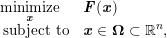
where
 $p>1$
objective functions
 $f_{i}:\mathbb{R}^{n}\rightarrow \mathbb{R}$
for
 $i=1,\ldots ,p$
define the vector-valued mapping
 $\boldsymbol{F}$
via
 $\boldsymbol{F}(\boldsymbol{x})=[f_{1}(\boldsymbol{x}),\ldots ,f_{p}(\boldsymbol{x})]$
. Given potentially conflicting objectives
 $f_{1},\ldots ,f_{p}$
, the problem (MOO) is well-defined only when given an ordering on the vector of objective values
 $\boldsymbol{F}(\boldsymbol{x})$
. Given distinct points
 $\boldsymbol{x}_{1},\boldsymbol{x}_{2}\in \mathbb{R}^{n}$
,
 $\boldsymbol{x}_{1}$
Pareto dominates
 $\boldsymbol{x}_{2}$
provided
 $$\begin{eqnarray}\displaystyle f_{i}(\boldsymbol{x}_{1})\leq f_{i}(\boldsymbol{x}_{2})\quad \text{for all }i=1,\ldots ,p\quad \text{and}\quad f_{j}(\boldsymbol{x}_{1})<f_{j}(\boldsymbol{x}_{2})\quad \text{for some }j. & & \displaystyle \nonumber\end{eqnarray}$$
The set of all feasible points that are not Pareto-dominated by any other feasible point is referred to as the Pareto(-optimal) set of (MOO). An in-depth treatment of such problems is provided by Ehrgott (Reference Ehrgott2005).
Ideally, a method designed for the solution of (MOO) should return an approximation of the Pareto set. If at least one objective
 $f_{1},\ldots ,f_{p}$
is non-convex, however, approximating the Pareto set can be challenging. Consequently, methods for multi-objective optimization typically pursue Pareto stationarity, which is a form of local optimality characterized by a first-order stationarity condition. If
 $\boldsymbol{\unicode[STIX]{x1D6FA}}=\mathbb{R}^{n}$
, a point
 $\boldsymbol{x}_{\ast }$
is a Pareto stationary point of
 $\boldsymbol{F}$
provided that for each
 $\boldsymbol{d}\in \mathbb{R}^{n}$
, there exists
 $j\in \{1,\ldots ,p\}$
such that
 $f_{j}^{\prime }(\boldsymbol{x}_{\ast };\boldsymbol{d})\geq 0$
. This notion of stationarity is an extension of the one given for single-objective optimization in (2.1).
Typical methods for (MOO) return a collection of points that are not known to be Pareto-dominated and thus serve as an approximation to the set of Pareto points. From a theoretical point of view, most methods endeavour only to demonstrate that all accumulation points are Pareto stationary, and rarely prove the existence of more than one such point. From a practical point of view, comparing the approximate Pareto sets returned by a method for multi-objective optimization is not straightforward. For discussions of some comparators used in multi-objective optimization, see Knowles and Corne (Reference Knowles and Corne2002) and Audet et al. (Reference Audet, Bigeon, Cartier, Le Digabel and Salomon2018a ).
Various derivative-free methods discussed in this survey have been extended to address (MOO). The method of Audet, Savard and Zghal (Reference Audet, Savard and Zghal2008b ) solves biobjective optimization problems by iteratively combining the two objectives into a single objective (for instance, by considering a weighted sum of the two objectives); MADS is then applied to this single-objective problem. Audet, Savard and Zghal (Reference Audet, Savard and Zghal2010) extend the method of Audet et al. (Reference Audet, Savard and Zghal2008b ) to multi-objective problems with more than two objectives. Audet et al. (Reference Audet, Savard and Zghal2008b , Reference Audet, Savard and Zghal2010) demonstrate that all refining points of the sequence of candidate points produced by these methods are Pareto stationary.
Custódio, Madeira, Vaz and Vicente (Reference Custódio, Madeira, Vaz and Vicente2011) propose direct-multisearch methods, a multi-objective analogue of direct-search methods. Like direct-search methods, direct-multisearch methods involve both a search step and a poll step. Direct-multisearch methods maintain a list of non-dominated points; at the start of an iteration, one non-dominated point must be selected to serve as the centre for a poll step. Custódio et al. (Reference Custódio, Madeira, Vaz and Vicente2011) demonstrate that at any accumulation point
 $\boldsymbol{x}_{\ast }$
of the maintained sequence of non-dominated points from a direct-multisearch method, it holds that for any direction
 $\boldsymbol{d}$
that appears in a poll step infinitely often,
 $f_{j}^{\prime }(\boldsymbol{x}_{\ast },\boldsymbol{d})\geq 0$
for at least one
 $j$
. In other words, accumulation points of the method are Pareto stationary when restricted to these directions
 $\boldsymbol{d}$
. Custódio and Madeira (Reference Custódio and Madeira2016) incorporate these direct-multisearch methods within a multistart framework in an effort to find multiple Pareto stationary points and thus to better approximate the Pareto set.
For stochastic biobjective problems, Kim and Ryu (Reference Kim and Ryu2011) employ sample average approximation to estimate
 $\boldsymbol{F}(\boldsymbol{x})=\mathbb{E}_{\boldsymbol{\unicode[STIX]{x1D709}}}[\tilde{\boldsymbol{F}}(\boldsymbol{x};\boldsymbol{\unicode[STIX]{x1D709}})]$
and propose a model-based trust-region method. Ryu and Kim (Reference Ryu and Kim2014) adapt the approach of Kim and Ryu (Reference Kim and Ryu2011) to the deterministic biobjective setting. At the start of each iteration, these methods construct fully linear models of both objectives around a (currently) non-dominated point. These methods solve three trust-region subproblems – one for each of the two objectives, and a third that weights the two objectives as in Audet et al. (Reference Audet, Savard and Zghal2008b
) – and accept all non-dominated trial points. If both objectives are in
 ${\mathcal{L}}{\mathcal{C}}^{1}$
, Ryu and Kim (Reference Ryu and Kim2014) prove that one of the three objectives satisfies a lim-inf convergence result of the form (2.5), implying the existence of a Pareto-stationary accumulation point.
Liuzzi, Lucidi and Rinaldi (Reference Liuzzi, Lucidi and Rinaldi2016) propose a method for constrained multi-objective non-smooth optimization that separately handles each objective and constraint via an exact penalty (see (7.2)) in order to determine whether a point is non-dominated. Given the non-sequential nature of how non-dominated points are selected, Liuzzi et al. (Reference Liuzzi, Lucidi and Rinaldi2016) identify and link the subsequences implied by a lim-inf convergence result. They show that limit points of these linked sequences are Pareto stationary provided the search directions used in each linked sequence are asymptotically dense in the unit sphere.
Cocchi, Liuzzi, Papini and Sciandrone (Reference Cocchi, Liuzzi, Papini and Sciandrone2018) extend implicit filtering to the multi-objective case. They approximate each objective gradient separately using implicit-filtering techniques; they combine these approximate gradients in a disciplined way to generate search directions. Cocchi et al. (Reference Cocchi, Liuzzi, Papini and Sciandrone2018) demonstrate that their method generates at least one accumulation point and that every such accumulation point is Pareto stationary.
8.5 Methods for multifidelity optimization
Multifidelity optimization concerns the minimization of a high-fidelity objective function
 $f=f_{0}$
in situations where a lower-fidelity version
 $f_{\unicode[STIX]{x1D716}}$
(for
 $\unicode[STIX]{x1D716}>0$
) also exists. Evaluations of the lower-fidelity function
 $f_{\unicode[STIX]{x1D716}}$
are less computationally expensive than are evaluations of
 $f_{0}$
; hence, a goal in multifidelity optimization is to exploit the existence of the lower-fidelity
 $f_{\unicode[STIX]{x1D716}}$
in order to perform as few evaluations of
 $f_{0}$
as possible. An example of such a setting occurs when there exist multiple grid resolutions defining discretizations for the numerical solution of partial differential equations that defines
 $f_{0}$
and
 $f_{\unicode[STIX]{x1D716}}$
.
Polak and Wetter (Reference Polak and Wetter2006) develop a pattern-search method that exploits the existence of multiple levels of fidelity. The method begins at the coarsest available level and then monotonically refines the level of fidelity (i.e. decreases
 $\unicode[STIX]{x1D716}$
) after a sufficient number of consecutive unsuccessful iterations occur.
A method that both decreases
 $\unicode[STIX]{x1D716}$
and increases
 $\unicode[STIX]{x1D716}$
(akin to the V- and W-cycles of multigrid methods (Xu and Zikatanov Reference Xu and Zikatanov2017)), is the multilevel method of Frandi and Papini (Reference Frandi and Papini2013). The method follows the MG/Opt framework of Nash (Reference Nash2000) and instantiates runs of a coordinate-search method at specified fidelity and solution accuracy levels. Another multigrid-inspired method is developed by Liu, Zeng and Yang (Reference Liu, Zeng and Yang2015), wherein a hierarchy of DIRECT runs are performed at varying fidelity and budget levels.
Model-based methods have also been extended to the multifidelity setting. For example, March and Willcox (Reference March and Willcox2012) employ a fully linear RBF model to interpolate the error between two different fidelity levels. Their method then employs this model within a trust-region framework, but uses
 $f_{0}$
to determine whether to accept a given step.
Another model-based approach for multifidelity optimization is co-kriging; see, for example, Xiong, Qian and Wu (Reference Xiong, Qian and Wu2013) and Le Gratiet and Cannamela (Reference Le Gratiet and Cannamela2015). In such approaches, a statistical surrogate (typically a Gaussian process model) is constructed for each fidelity level with the aim of modelling the relationships among the fidelity levels in areas of the domain relevant to optimization.
Derivative-free methods for multifidelity, multi-objective and concurrent/ parallel optimization remain an especially open avenue of future research.
Acknowledgements
We are grateful to referees and colleagues whose comments greatly improved the manuscript; these include Mark Abramson, Charles Audet, Ana Luísa Custódio, Sébastien Le Digabel, Warren Hare, Paul Hovland, Jorge Moré, Raghu Pasupathy, Margherita Porcelli, Francesco Rinaldi, Clément Royer, Katya Scheinberg, Sara Shashaani, Aekaansh Verma and Zaikun Zhang. We are especially indebted to Gail Pieper and Glennis Starling for their invaluable editing. This material is based upon work supported by the applied mathematics and SciDAC activities of the Office of Advanced Scientific Computing Research, Office of Science, US Department of Energy, under Contract DE-AC02-06CH11357.
Appendix Collection of WCC results
Table A.1 contains select WCC bounds for methods appearing in the literature. Given
 $\unicode[STIX]{x1D716}>0$
, all WCC bounds in this appendix are given in terms of
 $N_{\unicode[STIX]{x1D716}}$
, an upper bound on the number of function evaluations of a method to guarantee that the specified condition is met. We present results in this form because function evaluation complexity of derivative-free methods is often of greater interest than is iteration complexity. We present
 $N_{\unicode[STIX]{x1D716}}$
in terms of four parameters:
∙ the accuracy
$\unicode[STIX]{x1D716}$
;∙ the dimension
$n$
;∙ the Lipschitz constant of the function
$L_{\text{f}}$
, the Lipschitz constant of the function gradient
$L_{\text{g}}$
or the Lipschitz constant of the function Hessian
$L_{\text{H}}$
(provided these constants are well-defined); and∙ a measure of how far the starting point
$\boldsymbol{x}_{0}$
is from a stationary point
$\boldsymbol{x}_{\ast }$
. In this appendix, this measure is either
$f(\boldsymbol{x}_{0})-f(\boldsymbol{x}_{\ast })$
, (8.1)or$$\begin{eqnarray}R_{\text{level}}=\sup _{\boldsymbol{x}\in \mathbb{R}^{n}}\{\Vert \boldsymbol{x}-\boldsymbol{x}_{\ast }\Vert :f(\boldsymbol{x})\leq f(\boldsymbol{x}_{0})\}\end{eqnarray}$$
(8.2)$$\begin{eqnarray}R_{\boldsymbol{x}}\geq \Vert \boldsymbol{x}_{0}-\boldsymbol{x}_{\ast }\Vert .\end{eqnarray}$$




We present additional constants in
 $N_{\unicode[STIX]{x1D716}}$
when particularly informative.
Naturally, each method in Table A.1 has additional algorithmic parameters that influence algorithmic behaviour. We have omitted the dependence of each method’s WCC on the selection of algorithmic parameters to allow for an easier comparison of methods.
We recall that, with the exception of the methods from Nesterov and Spokoiny (Reference Nesterov and Spokoiny2017) and Konečný and Richtárik (Reference Konečný and Richtárik2014), the methods referenced in Table A.1 do not require knowledge of the value of the relevant Lipschitz constants.
Known WCC bounds on the number of function evaluations needed to achieve a given stationarity measure.
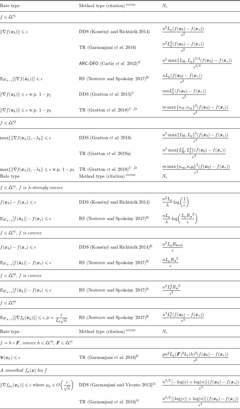
In Table A.1, we employ the constants
 $$\begin{eqnarray}\displaystyle p_{1} & = & \displaystyle \exp \biggl(-\displaystyle \frac{nL_{\text{g}}^{2}}{\unicode[STIX]{x1D716}^{2}}(f(\boldsymbol{x}_{0})-f(\boldsymbol{x}_{\ast }))\biggr),\nonumber\\ \displaystyle p_{2} & = & \displaystyle \exp \biggl(-\displaystyle \frac{\max {\{\unicode[STIX]{x1D705}_{\text{ef}},\unicode[STIX]{x1D705}_{\text{eg}}\}}^{2}}{\unicode[STIX]{x1D716}^{2}}(f(\boldsymbol{x}_{0})-f(\boldsymbol{x}_{\ast }))\biggr),\nonumber\\ \displaystyle p_{3} & = & \displaystyle \exp \biggl(-\displaystyle \frac{\max {\{\unicode[STIX]{x1D705}_{\text{eg}},\unicode[STIX]{x1D705}_{\text{eH}}\}}^{3}}{\unicode[STIX]{x1D716}^{3}}(f(\boldsymbol{x}_{0})-f(\boldsymbol{x}_{\ast }))\biggr).\nonumber\end{eqnarray}$$