1 Introduction
The interaction of a breaking wave with a vertical wall can be dramatic, significantly increasing the water velocity, especially if the interaction occurs during the inception of overturning. Breaking-wave impact creates turbulence and pockets of trapped air, generating a water jet when the steep wave front impacts the wall (Cooker & Peregrine Reference Cooker and Peregrine1995; Peregrine Reference Peregrine2003; Lugni, Brocchini & Faltinsen Reference Lugni, Brocchini and Faltinsen2006; Dias & Ghidaglia Reference Dias and Ghidaglia2018). Impact pressures increase with wave period (Goda Reference Goda1975). If the vertical wall has a finite height, overtopping can occur. Non-breaking waves may lead to a surge overtopping with a fast bore developing from the collapsing surge (Hansom, Barltrop & Hall Reference Hansom, Barltrop and Hall2008). What is less known is the interaction of long waves with a vertical wall. In this paper, we consider runup amplification of long waves at arbitrarily high walls, without the overtopping that may occur with a finite wall (Ryu, Chang & Mercier Reference Ryu, Chang and Mercier2007; Ryu & Chang Reference Ryu and Chang2008).
Runup amplification of shallow-water waves over a flat bathymetry can be significantly larger than that given by linear theory (factor of 5–6 as opposed to 2) due to a combination of reflection, constructive interference, dispersion and other nonlinear effects (Carbone et al. Reference Carbone, Dutykh, Dudley and Dias2013; Viotti, Carbone & Dias Reference Viotti, Carbone and Dias2014a ; Akrish et al. Reference Akrish, Schwartz, Rabinovitch and Agnon2016b ). Head-on solitary wave collisions produce large runup jets (Chambarel, Kharif & Touboul Reference Chambarel, Kharif and Touboul2009; Chen et al. Reference Chen, Kharif, Yang, Hsu, Touboul and Chambarel2015). Long wave packets usually disintegrate into a bore formation with smaller wavelengths (Akrish, Rabinovitch & Agnon Reference Akrish, Rabinovitch and Agnon2016a ; Akrish et al. Reference Akrish, Schwartz, Rabinovitch and Agnon2016b ; Brühl & Oumeraci Reference Brühl and Oumeraci2016; Trillo et al. Reference Trillo, Deng, Biondini, Klein, Clauss, Chabchoub and Onorato2016; Ning, Li & Zhang Reference Ning, Li and Zhang2018). Large runup amplifications are supported by higher frequencies in the spectrum. The resulting nonlinear interactions increase dynamic pressure, but reduce the peak force compared to linear theory. However, that force acts for a longer duration when multiple peaks develop (Brennan, Viotti & Dias Reference Brennan, Viotti and Dias2014; Akrish et al. Reference Akrish, Schwartz, Rabinovitch and Agnon2016b ). Interestingly, a varying bathymetry that becomes shallower closer to the wall further reduces the force during runup, as compared to the flat case, even though the amplification is greater (Brennan et al. Reference Brennan, Clancy, Harrington, Cox and Dias2017).
The influence of bathymetry on wave conditions is evident. In numerical simulations over a flat bathymetry, small-amplitude long waves do not exhibit breaking during runup at a wall. However, once a variable bathymetry is introduced, steep wave fronts develop. Furthermore, strong variations in depth enhance the amplification of waves (Viotti & Dias Reference Viotti and Dias2014; Bolles, Speer & Moore Reference Bolles, Speer and Moore2019). Waves can break, for example through the overturning of the wave crest. The onset of wave breaking is typically characterized by a steep asymmetric wave and the formation of whitewater (due to entrained air from turbulence) at the crest tip that falls down the face of the wave (Banner et al. Reference Banner, Barthelemy, Fedele, Allis, Benetazzo, Dias and Peirson2014; Kurnia & van Groesen Reference Kurnia and van Groesen2017). Wave breaking adds vorticity, turbulence and heat diffusion to the system (Longo et al. Reference Longo, Clavero, Chiapponi and Losada2017).
The physics of a breaking wave leads to several different criteria for determining the onset of wave breaking: geometric (Hwang, Xu & Wu Reference Hwang, Xu and Wu1989; Wu & Nepf Reference Wu and Nepf2002; Perlin, Choi & Tian Reference Perlin, Choi and Tian2013; Grue, Kolaas & Jensen Reference Grue, Kolaas and Jensen2014), kinematic (Hwang et al. Reference Hwang, Xu and Wu1989; Stansell & MacFarlane Reference Stansell and MacFarlane2002; Wu & Nepf Reference Wu and Nepf2002; Perlin et al. Reference Perlin, Choi and Tian2013) and energetic (Perlin et al. Reference Perlin, Choi and Tian2013; Seiffert, Ducrozet & Bonnefoy Reference Seiffert, Ducrozet and Bonnefoy2017; Barthelemy et al. Reference Barthelemy, Banner, Peirson, Fedele, Allis and Dias2018; Seiffert & Ducrozet Reference Seiffert and Ducrozet2018). These criteria are evaluated locally, as the extremal conditions for wave breaking may not be seen in global wave-parameter values. Wind forcing alters these conditions as it enhances wave steepness. However, this is only significant for strong winds acting over long scales (Babanin et al. Reference Babanin, Chalikov, Young and Savelyev2010). Wave breaking depends on the shape and/or motion of the free surface, which is altered by the wind (Hwang et al. Reference Hwang, Xu and Wu1989). Wind may act to delay the onset of breaking by supporting steeper waves (Iafrati, De Vita & Verzicco Reference Iafrati, De Vita and Verzicco2019), yet increase the frequency of breaking waves as the wind velocity increases (Xu, Hwang & Wu Reference Xu, Hwang and Wu1986). Dynamic criteria only change by a few percent as wind forcing and spectral bandwidth change (Saket et al. Reference Saket, Peirson, Banner, Barthelemy and Allis2017, Reference Saket, Peirson, Banner and Allis2018).
In this paper, we analyse the fundamental problem of long wave groups propagating towards vertical walls. We only determine the onset of wave breaking, as the numerical code for the Euler equations used cannot resolve beyond the breaking process. The breaking strength is strongly related to the onset of breaking (Derakhti, Banner & Kirby Reference Derakhti, Banner and Kirby2018). From this we may infer the wave behaviour in the zone where broken waves are present, such as whitecapping and plunging (Phillips Reference Phillips1985; Drazen, Melville & Lenain Reference Drazen, Melville and Lenain2008), without necessarily computing the flow. We consider the runup of a wave packet at a vertical wall over a simplified variable bathymetry, chosen as representative of the Aran Islands, Ireland. We briefly summarize preliminary results, presented at recent conferences, on wave breaking and runup. Furthermore, we consider additional and new measures of wave breaking and breaking strength. For non-breaking waves, nonlinear interactions among waves, vertical wall and bathymetry result in a maximum runup amplification that approaches a factor of 12 – large enough for a 3 m amplitude wave to overtop a 30 m cliff. Finally, we discuss the relevance of our results to the real world.
2 Model
2.1 Set-up
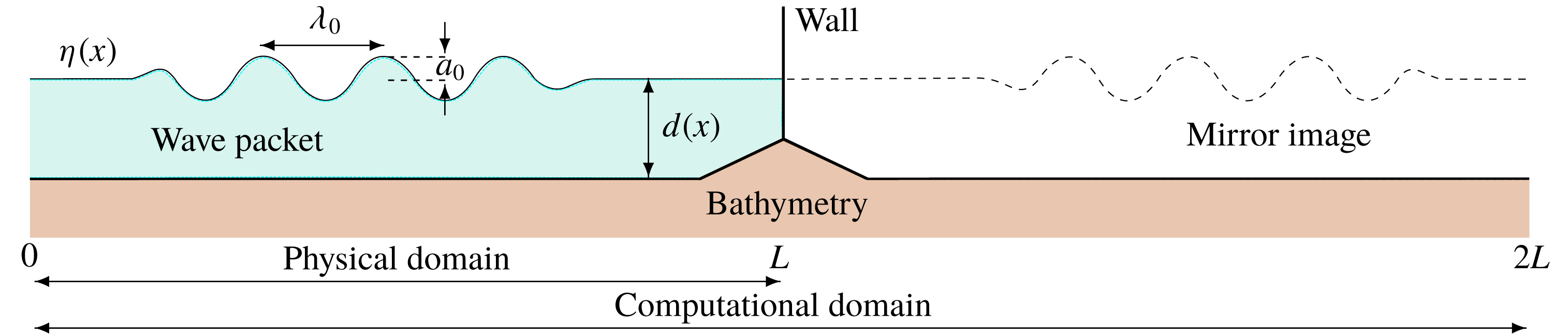
We consider the runup of a packet of long waves approaching a vertical wall over a variable bathymetry, with bathymetry profile given relative to the still-water depth
 $d(x)$
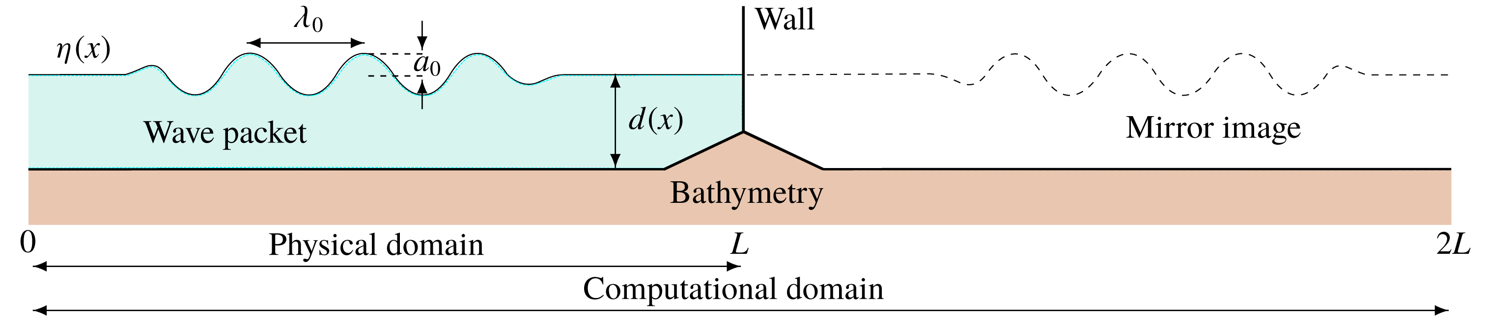
. A sketch of the set-up is shown in figure 1. We describe the wave packet’s motion by the incompressible Euler equations,
 $$\begin{eqnarray}\displaystyle & \unicode[STIX]{x1D6FB}^{2}\unicode[STIX]{x1D6F7}=0,\quad 0<x<2L,\quad -d(x)<y<\unicode[STIX]{x1D702}(x,t), & \displaystyle\end{eqnarray}$$
 $$\begin{eqnarray}\displaystyle & \unicode[STIX]{x1D702}_{t}=-\unicode[STIX]{x1D6F7}_{x}\unicode[STIX]{x1D702}_{x}+\unicode[STIX]{x1D6F7}_{y},\quad 0<x<2L,\quad y=\unicode[STIX]{x1D702}(x,t), & \displaystyle\end{eqnarray}$$
 $$\begin{eqnarray}\displaystyle & \unicode[STIX]{x1D6F7}_{t}=-{\textstyle \frac{1}{2}}(\unicode[STIX]{x1D6F7}_{x}^{2}+\unicode[STIX]{x1D6F7}_{y}^{2})-g\unicode[STIX]{x1D702},\quad 0<x<2L,\quad y=\unicode[STIX]{x1D702}(x,t), & \displaystyle\end{eqnarray}$$
 $$\begin{eqnarray}\displaystyle & \unicode[STIX]{x1D6F7}_{x}d_{x}+\unicode[STIX]{x1D6F7}_{y}=0,\quad 0<x<2L,\quad y=-d(x), & \displaystyle\end{eqnarray}$$
where
 $\unicode[STIX]{x1D702}(x,t)$
is the free surface,
 $\unicode[STIX]{x1D6F7}(x,y,t)$
is the velocity potential and
 $g$
is the acceleration due to gravity (Brennan et al.
Reference Brennan, Clancy, Harrington, Cox and Dias2017). Note that the water depth
 $d(x)>0$
, with
 $y=0$
the still-water level. The constant water depth far upstream where the bathymetry is flat is denoted by
 $h$
. We solve (2.1) with a conformal-mapping spectral method (Choi & Camassa Reference Choi and Camassa1999), using a mirror wave image to impose the wall boundary condition at
 $x=L$
and for periodicity (Viotti et al.
Reference Viotti, Carbone and Dias2014a
). Hence,
 $0<x<L$
is the physical domain and
 $0<x<2L$
is the computational domain, with periodic boundary conditions imposed at
 $x=0,\,2L$
(figure 1). The incoming wave packet experiences runup amplification,
 $R$
, at the vertical wall, given by
 $$\begin{eqnarray}R(t)=\frac{\unicode[STIX]{x1D702}(x=L,t)}{a_{0}},\end{eqnarray}$$
where
 $a_{0}$
is the initial amplitude of the incoming wave packet.
Sketch of model set-up with incoming wave packet
 $\unicode[STIX]{x1D702}(x)$
approaching a vertical wall over a variable bathymetry profile relative to the still-water depth
 $d(x)$
. The bathymetry is horizontal away from the wall, becoming shallower closer to shore. The waves have initial amplitude
 $a_{0}$
and wavelength
 $\unicode[STIX]{x1D706}_{0}$
. There are
 $N_{w}$
waves (crests and troughs) in each wave packet. The numerical method constructs a mirror image to simulate a vertical wall.
The waves we consider can be easily reproduced in laboratory experiments (Brühl & Oumeraci Reference Brühl and Oumeraci2016; Trillo et al.
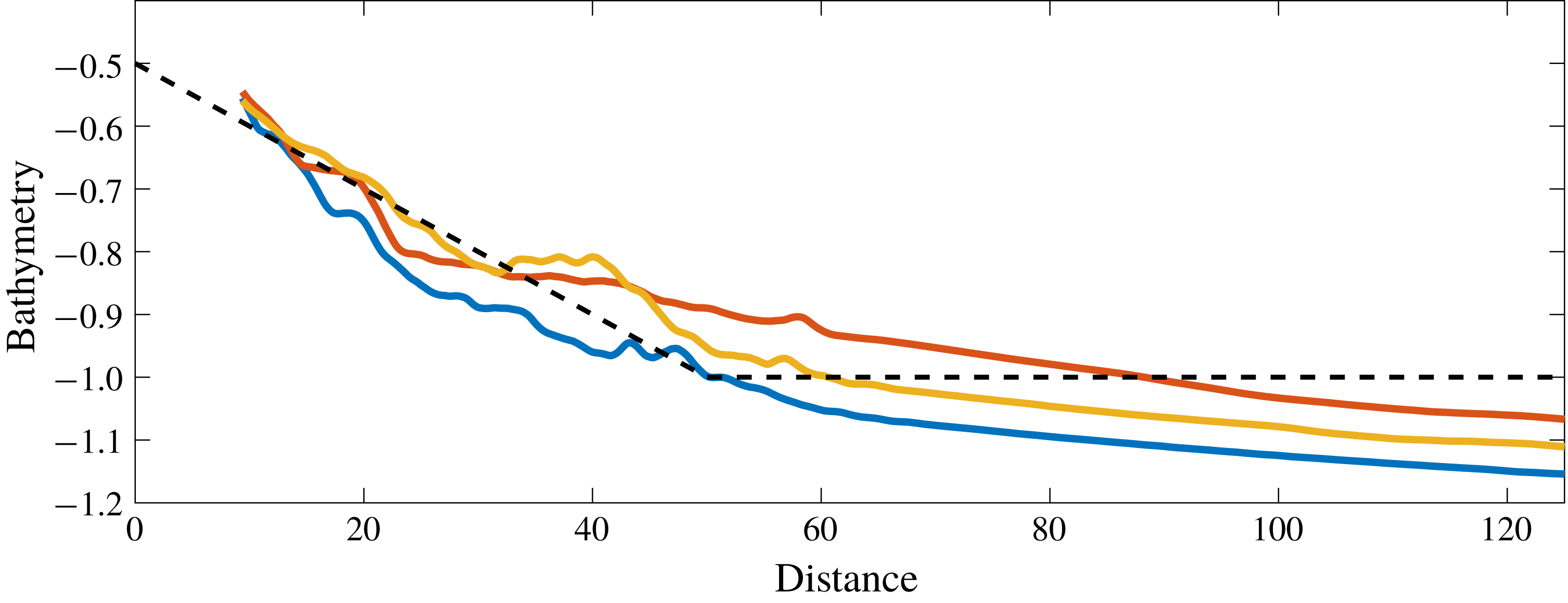
Reference Trillo, Deng, Biondini, Klein, Clauss, Chabchoub and Onorato2016). Their relevance to the real world is discussed in § 5. We use a bathymetry inspired by that of the Aran Islands off the west coast of Ireland. In figure 2 we show three transects (dimensionless, scaled by
 $h=80~\text{m}$
) taken with INSS and INFOMAR data from Geological Survey Ireland (2002--2016). We observe that the slope near the coast is an order of magnitude greater than that farther out. To represent this bathymetry, we approximate these data (dashed line in figure 2) as a piecewise-continuous linear function with a slope of 0.01 for the first 4 km from the coast, followed by a constant value. Considering an effective composite slope for the seabed is typical in the literature (Saville Jr Reference Saville1957; Mayer & Kriebel Reference Mayer and Kriebel1995). As bathymetry data are not available for closer than 750 m from the shoreline, we have extrapolated the bathymetry profile for our simplified approximation in this area. The depth at the cliffs is approximately 40 m and the ocean depth is approximately 80 m. Note that there is a tidal change of 5 m in this area. We address the effect of tidal differences by changing the location of the free surface, but keeping the bathymetry the same. We neglect the presence of any current.
From now on, all lengths are scaled with the constant ocean depth,
 $h=80~\text{m}$
, and time with
 $\unicode[STIX]{x1D70F}=(h/g)^{1/2}\approx 2.859~\text{s}$
. A laboratory replica of this situation at scale
 $1/100$
(water depth of 80 cm) would produce wave parameters (amplitude, period, water depth) quite similar to the values found in Brühl & Oumeraci (Reference Brühl and Oumeraci2016) and in Trillo et al. (Reference Trillo, Deng, Biondini, Klein, Clauss, Chabchoub and Onorato2016).
Three bathymetry transects (solid curves) perpendicularly to the western-side cliffs of Inis Mór. Image created from INSS and INFOMAR data from Geological Survey Ireland (2002--2016). The dashed line represents the idealized piecewise continuous representation of the bathymetry. The data are non-dimensionalized with respect to the typical depth,
 $h=80~\text{m}$
. Hence a 40 m (
 $=|-0.5|\times 80~\text{m}$
) depth at the cliff face and a flat bathymetry from 4 km (
 $=50\times 80~\text{m}$
). For a laboratory experiment at scale
 $1/100$
, the depth would be 40 cm at the wall and the flat bathymetry (80 cm) would start at 40 m from the wall.

We model an initial incoming wave packet, traversing from flat to non-flat bathymetry leading to the vertical wall (figure 1). The wave packet is well defined away from the wall, characterized by the following independent parameters: the number of waves
 $N_{w}$
, the initial amplitude
 $a_{0}$
and the period
 $P_{0}$
. Other parameters (angular frequency
 $\unicode[STIX]{x1D714}_{0}$
, wavenumber
 $k_{0}$
and wavelength
 $\unicode[STIX]{x1D706}_{0}$
) are related via common wave relations such as the dispersion relation. The initialized wave packet,
 $\unicode[STIX]{x1D702}_{0}(x)=\unicode[STIX]{x1D702}(x,t=0)$
and
 $\unicode[STIX]{x1D6F7}_{0}(x)=\unicode[STIX]{x1D6F7}(x,t=0)$
, is a sinusoidal group modulated by a hyperbolic tangent function (Viotti et al.
Reference Viotti, Carbone and Dias2014a
),
 $$\begin{eqnarray}\displaystyle & \unicode[STIX]{x1D702}_{0}(x)=a_{0}\cos [k_{0}(x-x_{0})]M(x)+\text{image}, & \displaystyle\end{eqnarray}$$
 $$\begin{eqnarray}\displaystyle & \unicode[STIX]{x1D6F7}_{0}(x)=a_{0}c(x)\coth [k_{0}d(x)]\sin [k_{0}(x-x_{0})]M(x)+\text{image}, & \displaystyle\end{eqnarray}$$
where
 $M(x)=1/2[\tanh ((x-x_{0})/\unicode[STIX]{x1D6FF})-\tanh ((x-x_{0}-N_{w}\unicode[STIX]{x1D706}_{0})/\unicode[STIX]{x1D6FF})]$
is a modulating function and
 $c(x)=[g\tanh (k_{0}d(x))/k_{0}]^{1/2}$
is a phase velocity. The subscript 0 refers to initial reference values and
 $\unicode[STIX]{x1D6FF}=\unicode[STIX]{x1D706}_{0}/6$
is a fitting factor. The runup of long-period cosine waves in shallow water has been the subject of experiments to understand the complex phenomena of near-shore dispersive breaking of long waves (Brühl & Oumeraci Reference Brühl and Oumeraci2016; Trillo et al.
Reference Trillo, Deng, Biondini, Klein, Clauss, Chabchoub and Onorato2016).
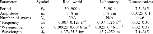
A summary of the wave parameter range is given in table 1. Note that the same symbol is used for dimensional and dimensionless variables. When there is ambiguity below, we specify whether it is the dimensional or the dimensionless value that is used. Since the combined parameter ranges could be reproduced in laboratory experiments, we simulate the full range, finding that large-amplitude long waves break up into wave trains as expected, and that those of the highest amplitudes always exhibit wave breaking. Though largely a theoretical exercise in these cases, we will see that it is the intermediate amplitude ranges of these high-amplitude wave packets that do not exhibit wave breaking and result in the highest runup amplifications. In the open ocean, tsunami waves can have wavelengths of 200 km and amplitude of 1 m in a depth of 4 km (Mader Reference Mader1974; Mei, Stiassnie & Yue Reference Mei, Stiassnie and Yue1989; Craig Reference Craig2006; Madsen, Fuhrman & Schäffer Reference Madsen, Fuhrman and Schäffer2008). We initialize our wave packet with long waves that have already developed to higher amplitudes (table 1) near the coast and propagate towards the coast where disintegration typically occurs (Madsen et al. Reference Madsen, Fuhrman and Schäffer2008). The initial wave packet of a modulated sinusoidal group evolves via a process of (i) steepening, (ii) undular bore formation and (iii) disintegration into solitons (Akrish et al. Reference Akrish, Rabinovitch and Agnon2016a ,Reference Akrish, Schwartz, Rabinovitch and Agnon b ; Brühl & Oumeraci Reference Brühl and Oumeraci2016; Trillo et al. Reference Trillo, Deng, Biondini, Klein, Clauss, Chabchoub and Onorato2016). The runup of such waves on a wall over a flat bathymetry has been characterized in the literature (Viotti et al. Reference Viotti, Carbone and Dias2014a ; Akrish et al. Reference Akrish, Rabinovitch and Agnon2016a ). Wave breaking is typically not observed for small amplitudes. The runup amplifications can be greater than six times the initial amplitude (Viotti et al. Reference Viotti, Carbone and Dias2014a ).
Parameter ranges for initial incoming wave packet. An asterisk signifies that the parameter is not independent but based on standard relations with the other parameters. The laboratory values are based on a
 $1/100$
scale.

2.2 Wave-breaking measures
Breaking waves are measured by a number of criteria, including geometry, kinematics and energy, following the characterizing overturning process. During the onset of wave breaking, the wave form may break down, e.g. whitecapping, spilling, plunging, with local steep crests and reduced phase speed, before overturning fully occurs (Schwendeman & Thomson Reference Schwendeman and Thomson2017). These processes are often reflected in practical criteria values; values that are lower than theoretical values. Furthermore, these are local events that are not always captured by global wave-parameter values. As such, local parameters are considered. In this section we describe some old and new wave-breaking criteria.
2.2.1 Geometric
The shape of the wave is an indicator for wave breaking, with many geometric metrics in use. These include crest front steepness, crest rear steepness, vertical and horizontal asymmetry factors (Wu & Tian Reference Wu and Tian2000; Wu & Nepf Reference Wu and Nepf2002; Perlin et al. Reference Perlin, Choi and Tian2013). Many critical values for each of these metrics have been proposed, beyond which breaking occurs. We consider the following metric for wave steepness:
 $$\begin{eqnarray}S=ka,\end{eqnarray}$$
measured locally at the crest tip. A typical critical value is
 $S_{crit}\approx 0.43$
(Melville Reference Melville1996; Wu & Nepf Reference Wu and Nepf2002; Toffoli et al.
Reference Toffoli, Babanin, Onorato and Waseda2010). The type of breaking wave (spilling, plunging) is related to the magnitude of
 $S$
, with steeper breaking waves more likely to be plunging than spilling (Perlin et al.
Reference Perlin, Choi and Tian2013). However, geometric criteria such as steepness have been criticized in the literature for their inconsistency (Barthelemy et al.
Reference Barthelemy, Banner, Peirson, Fedele, Allis and Dias2018). Non-breaking waves frequently attain steepness values that exceed those for breaking waves.
Ocean waves at finite depth are also measured with another geometric criterion, the ratio of wave height,
 $H_{w}$
, to depth,
 $d$
,
 $$\begin{eqnarray}H=\frac{H_{w}}{d}.\end{eqnarray}$$
Experimentally, the critical value for a horizontal seabed is
 $H_{crit}\approx 0.55$
(Riedel & Byrne Reference Riedel and Byrne1987; Nelson Reference Nelson1994; Grue et al.
Reference Grue, Kolaas and Jensen2014; Grue & Kolaas Reference Grue and Kolaas2017; Saket et al.
Reference Saket, Peirson, Banner and Allis2018). Other studies (Cyril & Galvin Reference Cyril and Galvin1972; Grilli, Svendsen & Subramanya Reference Grilli, Svendsen and Subramanya1997) suggest higher values, particularly for solitary waves; however, including higher-order approximations of the Stokes and cnoidal theories reduces them to at most the experimental critical value (Massel Reference Massel1996).
In the case of a seabed with a horizontal section followed by a slope, larger critical height-to-depth values (2.9) have been shown for random waves (Riedel & Byrne Reference Riedel and Byrne1987) and solitary waves (Munk Reference Munk1949; Grilli et al.
Reference Grilli, Svendsen and Subramanya1997). This depends on wave characteristics such as initial shape, breaking steepness, nonlinearities, bottom friction and the degree of the seabed slope (Munk Reference Munk1949; Goda Reference Goda1975). However, these bathymetry profiles form a beach. Beaches with larger slopes (such as 1 : 8) permit high values of
 $H>1$
(Munk Reference Munk1949; Saville Jr Reference Saville1957; Weggel Reference Weggel1973), whereas lower gradient beaches (such as 1 : 100) retain the condition
 $H<0.55$
(Riedel & Byrne Reference Riedel and Byrne1987). Furthermore, the critical
 $H$
decreases with depth-to-wavelength ratio, so that shorter-period waves have smaller breaking heights. Many empirically derived functional formulae for
 $H$
, incorporating beach slope and wavelength, have been proposed (Goda Reference Goda1975, Reference Goda2010).
In our case waves propagate over a slope of 1 : 100 until they reach a vertical wall (figures 1 and 2). Wave interaction with the wall can occur without wave breaking, resulting in incoming and reflecting wave–wave interactions that significantly amplify subsequent waves. This bathymetry-induced amplification is implicit in the steepness (2.8), but explicit in the wave height-to-depth ratio (2.9).
2.2.2 Kinematic
Physically, wave breaking occurs if the local fluid particle velocity,
 $|\boldsymbol{U}|$
, exceeds the local wave phase velocity,
 $C$
. The kinematic breaking measure is the ratio
 $$\begin{eqnarray}K=\frac{|\boldsymbol{U}|}{C},\end{eqnarray}$$
with theoretical breaking condition
 $K_{crit}\geqslant 1$
. Studies estimate the kinematic criterion (2.10) to be lower than 1 due to the onset of breaking (Wu & Nepf Reference Wu and Nepf2002; Kurnia & van Groesen Reference Kurnia and van Groesen2017; Barthelemy et al.
Reference Barthelemy, Banner, Peirson, Fedele, Allis and Dias2018). For practical reasons, such as the inability to resolve wave evolution after the onset of breaking, the criterion (2.10) may be taken to be as low as
 $K_{crit}\geqslant 0.7$
(Wu & Nepf Reference Wu and Nepf2002; Perlin et al.
Reference Perlin, Choi and Tian2013). The type of breaking wave (spilling, plunging) is related to the magnitude of
 $K$
, with
 $K_{crit}^{plunging}>K_{crit}^{spilling}$
. However, the exact values are not well defined (Perlin et al.
Reference Perlin, Choi and Tian2013). We consider critical values as defined by Wu & Nepf (Reference Wu and Nepf2002) as we compute velocities based on their formulation. They suggest spilling occurs for
 $K>1$
and plunging for
 $K>1.5$
.
The fluid velocity,
 $|\boldsymbol{U}|$
, is derived from the local velocity field,
 $\text{}\text{u}=(u,v)$
,
 $$\begin{eqnarray}|\boldsymbol{U}|=(u^{2}+v^{2})^{1/2}=(\unicode[STIX]{x1D6F7}_{x}^{2}+\unicode[STIX]{x1D6F7}_{y}^{2})^{1/2}.\end{eqnarray}$$
The phase velocity,
 $C$
, is given by the local wave parameters of angular frequency,
 $\unicode[STIX]{x1D714}$
, and wavenumber,
 $k$
,
 $$\begin{eqnarray}C=\frac{\unicode[STIX]{x1D714}}{|k|}=\left(\frac{g\tanh (kd)}{k}\right)^{1/2},\end{eqnarray}$$
via the dispersion relation
 $\unicode[STIX]{x1D714}^{2}=gk\tanh (kd)$
, for depth
 $d$
. For our study,
 $d=d(x)$
is spatially varying (figure 2). The local wavenumber,
 $k$
, takes the form of the gradient of the phase, given by
 $$\begin{eqnarray}k=\frac{\unicode[STIX]{x1D702}\unicode[STIX]{x1D701}_{x}-\unicode[STIX]{x1D702}_{x}\unicode[STIX]{x1D701}}{\unicode[STIX]{x1D702}^{2}+\unicode[STIX]{x1D701}^{2}},\end{eqnarray}$$
where
 $\unicode[STIX]{x1D701}$
is the conjugate to the free surface (Stansell & MacFarlane Reference Stansell and MacFarlane2002; Kurnia & van Groesen Reference Kurnia and van Groesen2014).
An alternative method is to first calculate the local angular frequency
 $\unicode[STIX]{x1D714}$
, with the wavenumber
 $k$
given by the dispersion relation (Stansell & MacFarlane Reference Stansell and MacFarlane2002; Wu & Nepf Reference Wu and Nepf2002; Kurnia & van Groesen Reference Kurnia and van Groesen2014).
2.2.3 Energetic
A new energy breaking criterion has been proposed by Barthelemy et al. (Reference Barthelemy, Banner, Peirson, Fedele, Allis and Dias2018). The criterion is based on the local normalized energy flux for deep and intermediate water depths, evaluated at the crest tip of a wave. The concept is that the wave cannot accommodate a local energy flux beyond that in the corresponding maximum recurrent case. Let
 $p$
denote the pressure relative to the atmospheric pressure. The criterion is a ratio,
 $B$
, between the local energy flux,
 $\text{}\text{F}=\text{}\text{u}(p+y+{\textstyle \frac{1}{2}}||\text{}\text{u}||^{2})$
, and the local energy density,
 $E=y+{\textstyle \frac{1}{2}}||\text{}\text{u}||^{2}$
, given by
 $$\begin{eqnarray}B=\frac{||\text{}\text{F}||}{E|c|},\end{eqnarray}$$
where
 $c=-\unicode[STIX]{x1D702}_{xt}/\unicode[STIX]{x1D702}_{xx}$
is the crest speed (Fedele Reference Fedele2014). The crest speed arises from following the evolution of the crest tip
 $x_{c}(t)$
, formally given by
 $c=\text{d}x_{c}/\text{d}t$
(Stansell & MacFarlane Reference Stansell and MacFarlane2002). It is found that, for a flat bottom with deep to intermediate depth, the criterion for the onset of breaking is
 $0.85<B_{crit}<0.86$
(Barthelemy et al.
Reference Barthelemy, Banner, Peirson, Fedele, Allis and Dias2018). This threshold increases by only a few percent as wind forcing becomes significant, decreases by a few percent as the spectral bandwidth increases and is unaffected by wavelength (Saket et al.
Reference Saket, Peirson, Banner, Barthelemy and Allis2017, Reference Saket, Peirson, Banner and Allis2018). At the free surface,
 $z=\unicode[STIX]{x1D702}$
, where
 $p=0$
, the flux breaking metric (2.14) reduces to
 $B=|\boldsymbol{U}|/|c|$
. This is a similar measure to the kinematic criterion (2.10); however a dynamic leaning cycle during propagation results in a crest slowdown. This slowdown is observed by a probability density function centred at about 80 % of the phase speed (Banner et al.
Reference Banner, Barthelemy, Fedele, Allis, Benetazzo, Dias and Peirson2014; Fedele Reference Fedele2014).
The results in Barthelemy et al. (Reference Barthelemy, Banner, Peirson, Fedele, Allis and Dias2018) are computed for waves that have reached, and are propagating at, their maximum height, so that no vertical component exists. During reflection of the wave at the vertical wall, however,
 $c\rightarrow 0$
as the crest changes direction, while
 $|\boldsymbol{U}|\not \rightarrow 0$
during runup due to the vertical velocity component. Hence,
 $B\rightarrow \infty$
during the period of most interest. For this reason, we do not explicitly calculate
 $B$
. Instead, we use the above observation of its relation to the phase speed (
 $c\approx 0.8C$
) to write
 $$\begin{eqnarray}B\approx \frac{5}{4}\frac{|\boldsymbol{U}|}{C}=\frac{5}{4}K.\end{eqnarray}$$
The range
 $0.85<B_{crit}<0.86$
is close to
 ${\textstyle \frac{5}{4}}K_{crit}\approx 0.875$
.
2.2.4 Breaking strength
After a wave breaks, energy is dissipated (Duncan Reference Duncan1983). This leads to a dimensionless measure of the breaking strength
 $b$
,
 $$\begin{eqnarray}b=\frac{g\tilde{\unicode[STIX]{x1D716}}}{\unicode[STIX]{x1D70F}_{b}l\unicode[STIX]{x1D70C}c_{b}^{5}},\end{eqnarray}$$
given in terms of the total energy dissipation
 $\tilde{\unicode[STIX]{x1D716}}$
, fluid density
 $\unicode[STIX]{x1D70C}$
and characteristic scales of a breaking wave such as active breaking period
 $\unicode[STIX]{x1D70F}_{b}$
, mean length
 $l$
of the breaking crest and phase speed
 $c_{b}$
of the breaking wave (Phillips Reference Phillips1985; Drazen et al.
Reference Drazen, Melville and Lenain2008).
Computing the total energy dissipation
 $\tilde{\unicode[STIX]{x1D716}}$
of an isolated breaking event requires simulating the event beyond the breaking point. However, Derakhti et al. (Reference Derakhti, Banner and Kirby2018) show that the breaking strength is related to the rate of change of the normalized energy flux parameter
 $B$
(2.14),
 $$\begin{eqnarray}b=b\left(\frac{\text{d}B}{\text{d}t}\right).\end{eqnarray}$$
The breaking strength increases with
 $\text{d}B/\text{d}t$
. It is observed numerically that as
 $B$
approaches its critical breaking value, the type of breaking depends on its rate of change. Plunging occurs for larger values of
 $\text{d}B/\text{d}t$
than spilling (Derakhti et al.
Reference Derakhti, Banner and Kirby2018). We will compute
 $\text{d}B/\text{d}t$
during the onset of breaking and use it to characterize the breaking strength of long-wave wave packets.
3 Numerical methodology
We solve the Euler equations (2.1)–(2.4) with initial conditions (2.6) and (2.7) numerically, using a spectral conformal-mapping method. For a dimensionless system, the maximum depth is 1, and we take
 $g=1$
(Viotti, Dutykh & Dias Reference Viotti, Dutykh and Dias2014b
).
The spectral conformal-mapping method maps the problem from the physical domain of a propagating wave over a spatially varying bathymetry to a finite strip (Choi & Camassa Reference Choi and Camassa1999; Viotti et al.
Reference Viotti, Carbone and Dias2014a
,Reference Viotti, Dutykh and Dias
b
). The simulation is run with
 $N=16\,384$
Fourier modes, with half the spectrum dealiased, giving suitable convergence (Brennan et al.
Reference Brennan, Clancy, Harrington, Cox and Dias2017). Runup amplification at a vertical wall over a varying bathymetry compares well with other codes (Benoit et al.
Reference Benoit, Dias, Herterich and Scolan2018). The physical domain (half the computational domain due to the mirror image) is
 $L=50+(2+N_{w})\unicode[STIX]{x1D706}_{0}$
where 50 is the dimensionless length of the sloped region of the bathymetry (figure 2). The wave packet is initiated with its leading edge
 $1.5\unicode[STIX]{x1D706}_{0}$
from the sloped region of the bathymetry (figure 1). The run time varies with each wave packet, allowing enough time for the waves to reach the vertical wall and fully reflect.
The initial wave packet (2.6) is not an exact solution of the problem, leading to a small transient adjustment. Furthermore, this imposed initial condition allows for the development of the undular bore and disintegration into solitons (Akrish et al. Reference Akrish, Rabinovitch and Agnon2016a ,Reference Akrish, Schwartz, Rabinovitch and Agnon b ; Brühl & Oumeraci Reference Brühl and Oumeraci2016; Trillo et al. Reference Trillo, Deng, Biondini, Klein, Clauss, Chabchoub and Onorato2016).
Solving the Euler equations (2.1)–(2.4) yields the time and space evolution of the free surface,
 $\unicode[STIX]{x1D702}(x,t)$
, and the velocity potential,
 $\unicode[STIX]{x1D6F7}(x,y,t)$
. The crests and troughs are easily identified, with the amplitude
 $a$
given by the crest height. The conjugate to the free surface,
 $\unicode[STIX]{x1D701}$
, is calculated via a partial Hilbert transform with respect to
 $x$
,
 $$\begin{eqnarray}\unicode[STIX]{x1D701}(x,t)={\mathcal{H}}[\unicode[STIX]{x1D702}]=\frac{1}{\unicode[STIX]{x03C0}}\,\text{p.v.}\int _{-\infty }^{\infty }\frac{\unicode[STIX]{x1D702}(\unicode[STIX]{x1D712},t)}{x-\unicode[STIX]{x1D712}}\,\text{d}\unicode[STIX]{x1D712},\end{eqnarray}$$
where p.v. indicates the principal value of the integral (Stansell & MacFarlane Reference Stansell and MacFarlane2002). This integral is a convolution of
 $\unicode[STIX]{x1D702}$
and
 $1/\unicode[STIX]{x03C0}\,x$
. As such, the computation may be greatly simplified using the convolution theorem, such that
 $$\begin{eqnarray}{\mathcal{F}}[{\mathcal{H}}[\unicode[STIX]{x1D702}]](\unicode[STIX]{x1D708})=-\text{i}\,\text{sgn}(\unicode[STIX]{x1D708}){\mathcal{F}}[\unicode[STIX]{x1D702}](\unicode[STIX]{x1D708}),\end{eqnarray}$$
since
 ${\mathcal{F}}[1/\unicode[STIX]{x03C0}\,x](\unicode[STIX]{x1D708})=-\text{i}\,\text{sgn}(\unicode[STIX]{x1D708})$
. As a spectral method is used to solve the Euler equations (2.1)–(2.4), the Fourier transform of the free surface is computed, producing the Fourier coefficients in the conformal space. When calculating spatial derivatives, the chain rule and Cauchy–Riemann equations are used to appropriately calculate derivatives in physical space. Note that in the above calculations, the Fourier and Hilbert transforms are computed with respect to their discrete forms at each time step.
The breaking criteria are all computed with regard to local parameter values. We only consider those values at the crest tips. Whereas some studies (Barthelemy et al. Reference Barthelemy, Banner, Peirson, Fedele, Allis and Dias2018) consider only the crest tips at the highest attained elevation, with no vertical velocity component, we follow the crest tips throughout their evolution. This is necessary as the varying bathymetry significantly influences the amplitude throughout its evolution. However, we restrict (filter) consideration of certain crests via two conditions: (i) crests that are at least 10 % larger in amplitude than nearby crests, (ii) crests with amplitudes that are at least 50 % the initial amplitude. The first condition filters the smaller-amplitude crests on a wave train. The second condition filters waves with near-zero surface displacement that result in an artificial blowup of the criteria.
The wave height,
 $H_{w}$
, is calculated at the crest peaks throughout the evolution of the wave packet. We determine
 $H_{w}$
based on the trough in front of each crest. That is, we consider the direction (towards or away from the vertical wall) in which each crest is travelling and use the trough ahead of it. We determine the direction of the wave by the sign of the horizontal velocity component.
The runup amplification is only considered for non-breaking waves. Since we cannot solve for the wave evolution beyond breaking (Viotti et al. Reference Viotti, Carbone and Dias2014a ), we do not know the full extent of runup amplification. This is highlighted by studies suggesting that the runup of breaking waves may contain water jets due to high pressures and trapped air (Peregrine Reference Peregrine2003).
Finally, in the case of breaking waves, we compute the criteria during the onset of breaking at finer (
 $\times 100$
) time intervals than throughout the simulation. This provides a more accurate measure for critical values. The breaking strength parameter (2.17) is computed with a simple finite-difference discretization.
4 Results
4.1 Wave evolution
We solve the Euler equations (2.1)–(2.4) for the free surface
 $\unicode[STIX]{x1D702}$
and velocity potential
 $\unicode[STIX]{x1D6F7}$
, with initial conditions (2.6) and (2.7) taking parameter values in table 1. Typically, the large amplifications of crests occur during wave–wave and wave–wall interactions, with bathymetry playing a significant role. The wave packet breaks up into a wave train near the wall (Herterich & Dias Reference Herterich and Dias2017a
), as expected from long waves propagating towards a shore (Madsen & Fuhrman Reference Madsen and Fuhrman2008; Madsen et al.
Reference Madsen, Fuhrman and Schäffer2008; Brühl & Oumeraci Reference Brühl and Oumeraci2016; Trillo et al.
Reference Trillo, Deng, Biondini, Klein, Clauss, Chabchoub and Onorato2016).
We begin by examining wave breaking during wave evolution. We quantify the process by the various criteria as discussed in § 2.2, and treat breaking and non-breaking waves differently. We determine a measure of the breaking strength (2.17). For non-breaking waves, we measure the runup amplification
 $R$
(2.5), a local measure of wave interaction with a wall and consider extreme waves that reach the wall.
4.2 Wave breaking
4.2.1 Summary of preliminary results
The evolution of wave packets, as described, often results in a breakdown of the numerical solver. We establish that this is a result of the physical phenomenon of wave breaking. As this is not captured in our model, the solver cannot resolve the wave form.
We simulate wave packets with initial conditions from table 1, especially parameter values about where the waves appear to transition from non-breaking to breaking. The waves with greatest steepness
 $S$
(2.8), wave height-to-depth ratio
 $H$
(2.9), kinematic
 $K$
(2.10), and, by inference, energetic
 $B$
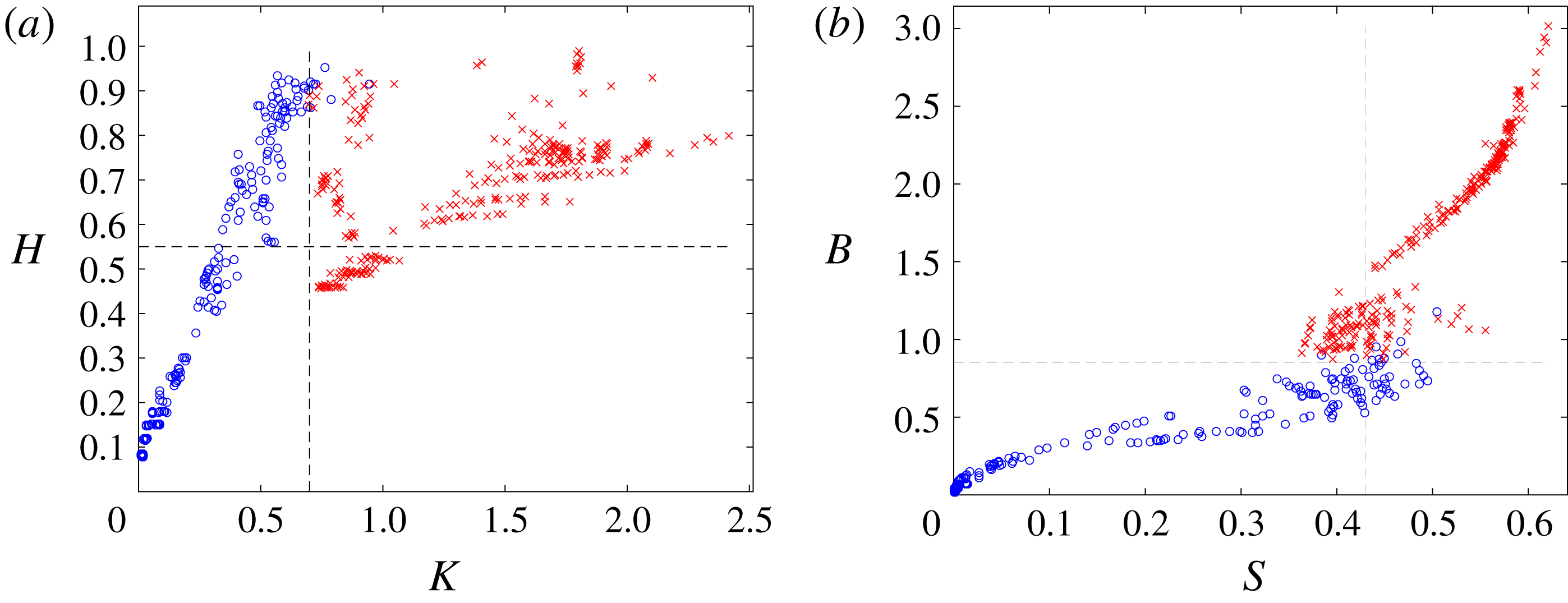
(2.15) measures are determined for each simulation. Comparisons of the different measures are shown in figure 3, with more simulations performed than reported in Herterich & Dias (Reference Herterich and Dias2017a
,Reference Herterich and Dias
b
).
Comparison of steepness
 $S$
(2.8), wave height-to-depth ratio
 $H$
(2.9), kinematic
 $K$
(2.10), and energetic
 $B$
(2.15) wave-breaking measures. We distinguish between non-breaking (○) and breaking (
 $\times$
) waves. Each marker represents a simulation with initial conditions from table 1. (a) Height-to-depth ratio and kinematic. (b) Energetic and steepness. The dashed lines are accepted critical values.

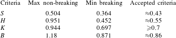
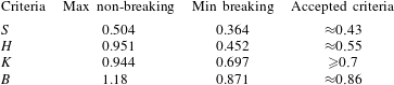
As discussed, there is often inconsistency in both geometric measures; non-breaking waves which exceed typical criteria values, and vice versa, as often reported. The critical ranges are summarized in table 2. There are many non-breaking waves that significantly exceed the critical values. However, in the kinematic case, the maximum (0.951) is still below the theoretical critical value of 1. We will analyse these waves in more detail in the subsequent sections of the paper. However, the lower bounds for breaking by the kinematic and energetic measures are consistent with the literature (Wu & Nepf Reference Wu and Nepf2002; Barthelemy et al. Reference Barthelemy, Banner, Peirson, Fedele, Allis and Dias2018).
There is a clear linear trend in the relationships among geometric (
 $S$
and
 $H$
), kinematic (
 $K$
) and energetic (
 $B$
) measures for non-breaking waves. The kinematic and energetic measures best adhere to the accepted criteria. The dimensionless amplitude
 $a_{0}$
and number of waves
 $N_{w}$
are the biggest factors related to wave breaking, as discussed in Herterich & Dias (Reference Herterich and Dias2017a
). These influence the wave–wave interactions that amplify and steepen waves, similar to the flat case (Carbone et al.
Reference Carbone, Dutykh, Dudley and Dias2013). For example, the amplitude above which breaking usually occurs can be up to 50 % higher for
 $N_{w}=1$
(dimensionless amplitude
 $a_{0}>0.063$
) than
 $N_{w}>1$
(dimensionless amplitude
 $a_{0}>0.043$
).


4.2.2 Breaking strength
The breaking strength is related to the onset of breaking via the energetic measure
 $B$
(2.15), as discussed in § 2.2.4. The breaking strength parameter also takes the form
 $b=b(\text{d}B/\text{d}t)$
(2.17). We observe the quantity
 $\text{d}B/\text{d}t$
to increase with
 $B$
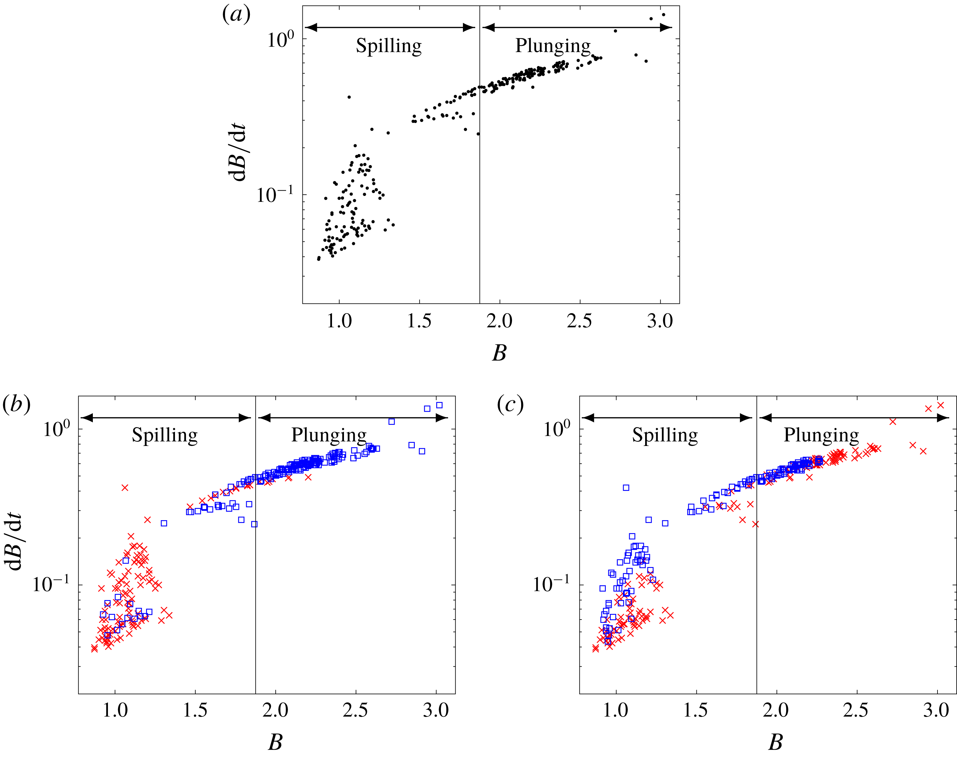
(figure 4). As
 $B$
is a measure of energy flux, we expect more energetic fluxes to have larger breaking strengths. The values of
 $\text{d}B/\text{d}t$
obtained are of similar order of magnitude to the
 $\unicode[STIX]{x1D6E4}\propto \,\text{d}B/\text{d}t$
in figure 5 of Derakhti et al. (Reference Derakhti, Banner and Kirby2018). Note that we neglect the scaling in the proportionality for
 $\unicode[STIX]{x1D6E4}$
as our simulations are already dimensionless.
(a) The rate of change of
 $B$
(2.15) for breaking waves, an indicator of the breaking strength for all waves. In (b,c) we group the results in (a) with respect to initial wave amplitude and period: (b)
 $0.04<a_{0}<0.06$
(
 $\times$
) and
 $0.06<a_{0}<0.1$
(▫); (c)
 $P_{0}<210$
(
 $\times$
) and
 $210<P_{0}<315$
(▫). The ranges for the types of breaking (spilling and plunging) are from Wu & Nepf (Reference Wu and Nepf2002), converted from a condition on
 $K$
to
 $B$
, via (2.15).

Classifying the initial waves that correspond to each simulation in figures 3 and 4 is relatively simple. In general, all measures
 $S$
,
 $H$
,
 $K$
,
 $B$
and
 $\text{d}B/\text{d}t$
increase with initial amplitude
 $a_{0}$
and decrease with period
 $P_{0}$
, as expected. This is in agreement with experiments (Goda Reference Goda1975, Reference Goda2010). The initial wave profile has an effect on the final breaking strength. Waves with greater initial amplitudes are more likely to result in plunging (figure 4
b). However, for wave periods it is less clear (figure 4
c). There are similar numbers of waves that exhibit plunging as well as spilling for all initial wave periods. Note that many long waves break up into wave trains with smaller periods.
4.3 Runup amplification
4.3.1 Summary of preliminary results
Each wave in the wave packet is amplified at the wall. However, we consider a single parameter to represent the runup in each simulation (from table 1), the maximum runup amplification,
 $$\begin{eqnarray}R_{max}=\max (R(t)).\end{eqnarray}$$
In general,
 $R_{max}$
increases with the amplitude of the initial wave packet. As we do not know the subsequent wave evolution for breaking waves, after the onset of breaking, we do not consider these waves here. Typically, waves break for
 $a_{0}>0.04$
(Herterich & Dias Reference Herterich and Dias2017a
). The runup amplification steadies out with respect to
 $N_{w}$
for
 $N_{w}\geqslant 3$
, as for a flat bathymetry (Viotti et al.
Reference Viotti, Carbone and Dias2014a
).
Increasing the bathymetry slope (figure 1) from flat to 1 % almost doubles the runup amplification, with
 $R_{max}>10$
in all cases. Dimensionally, this means that a wave packet of initial amplitude 3 m can overtop a 30 m cliff in ocean-type conditions. In the laboratory, that would correspond to a 3 cm wave overtopping a 30 cm cliff.
4.3.2 Tidal effects
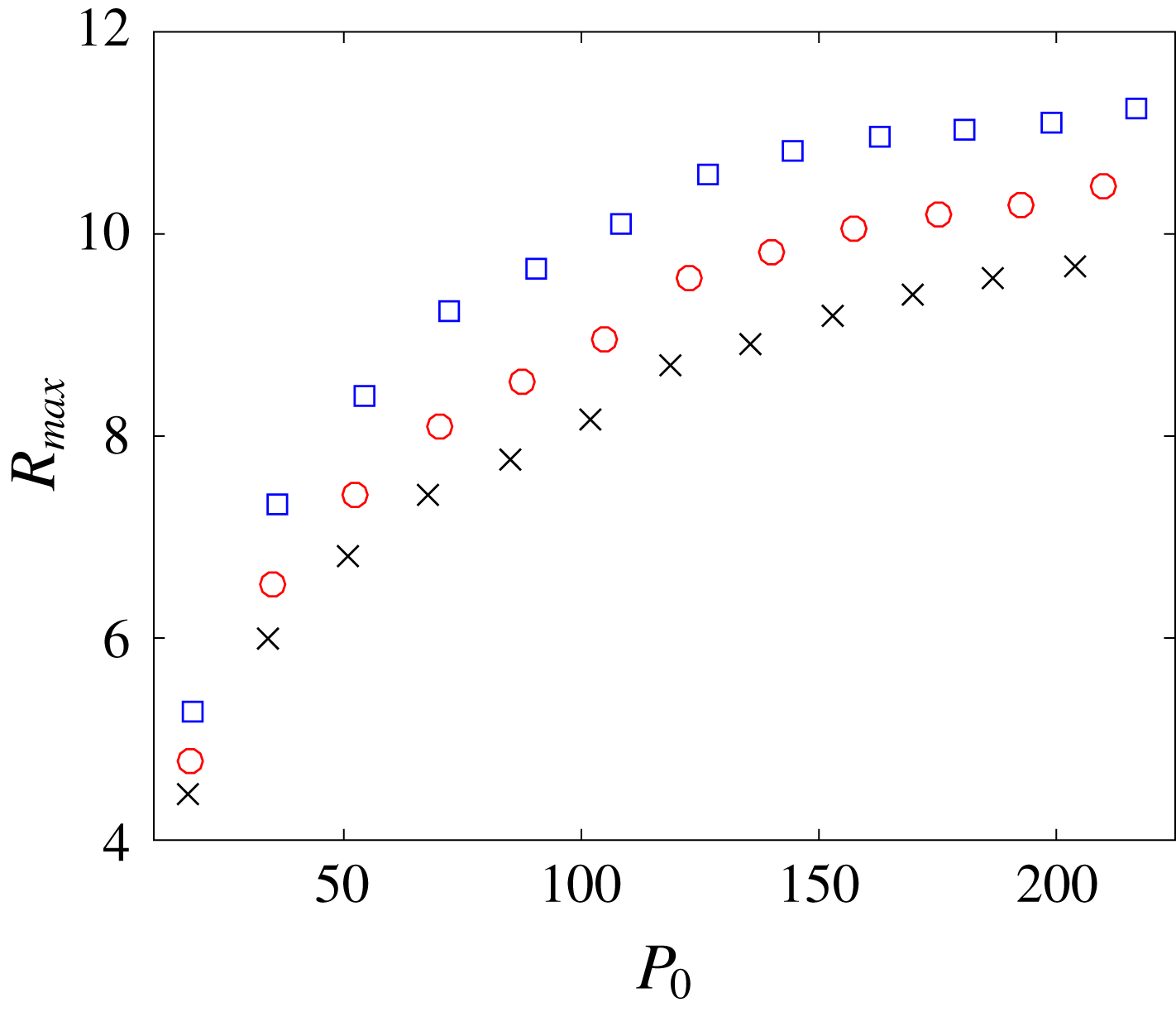
The tide affects the absolute depth over a bathymetry profile. While the bathymetry clearly is important in runup amplification, changes in the tide can increase or decrease its influence. Decreasing the free-surface height by a constant of 5 m increases
 $R_{max}$
by approximately 1 (figure 5). Furthermore, the runup amplification increases with increasing period, from 4 to
 $9+$
, until
 $P_{0}=140$
, when increases are at a slower rate.
Maximum runup amplification
 $R_{max}$
(4.1) against initial wave period
 $P_{0}$
for different tidal levels with the same underlying Aran Islands bathymetry (figure 2). The ocean depth is taken to be
 $h=75~\text{m}$
(▫), 80 m (○) and 85 m (
 $\times$
). All wave packets are initialized dimensionally with respect to the new depths (numbers in table 1 are with respect to
 $h=80~\text{m}$
), and with
 $N_{w}=3$
and
 $a_{0}=0.04$
.

Runup amplification,
 $R(t)$
, as a function of the dimensionless time
 $t$
for three different bathymetries: flat, flat followed by a 1 : 200 slope, flat followed by a 1 : 100 slope. The 1 % slope represents the Aran Islands bathymetry (figure 2). In all simulations
 $P_{0}=140,N_{w}=3,a_{0}=0.04$
.

4.3.3 Extreme waves
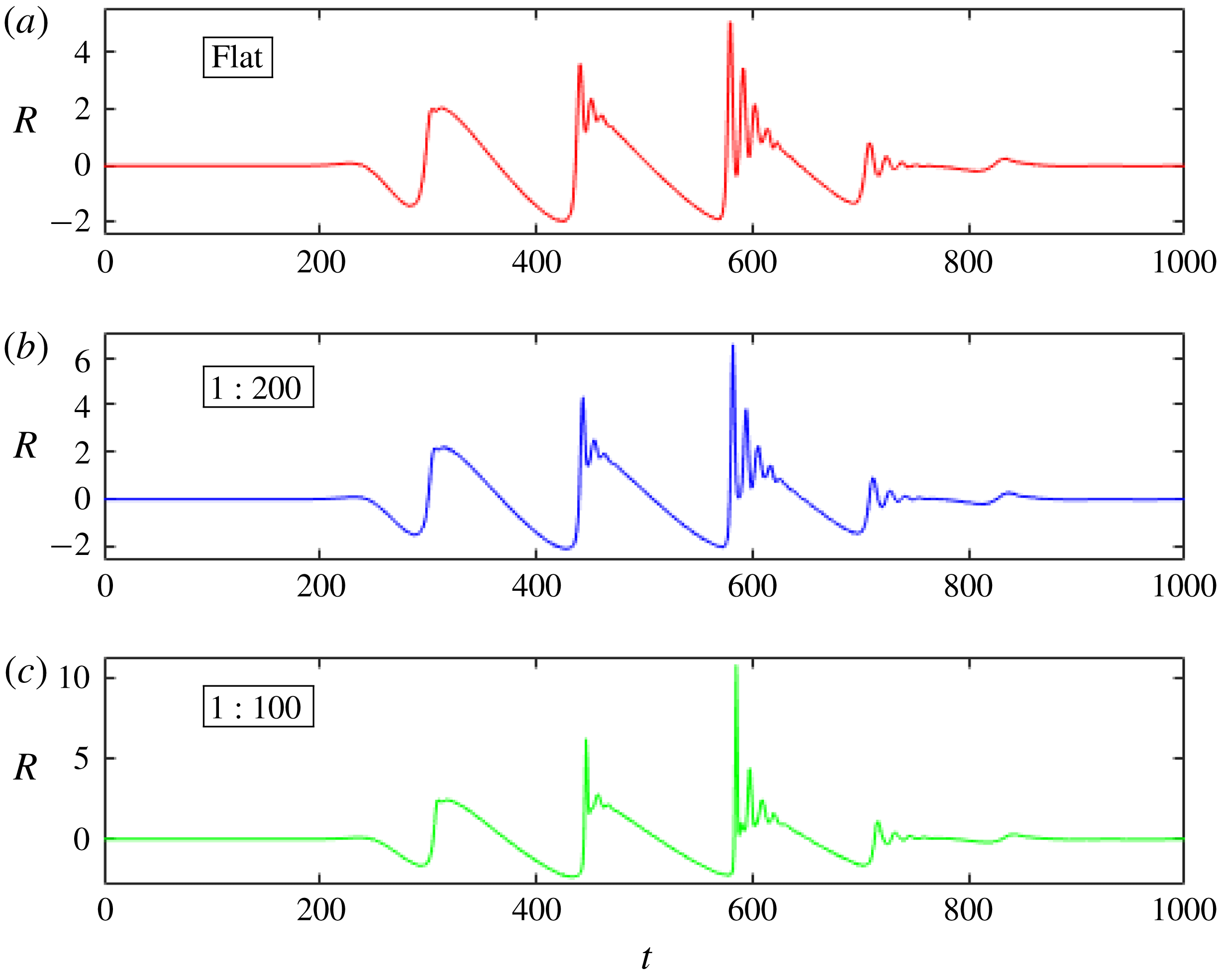
As discussed, the bathymetry plays a crucial role in runup amplification of waves. In figure 6, we show the runup
 $R(t)$
for a wave packet with dimensionless parameters
 $(P_{0},N_{w},a_{0})=(140,3,0.04)$
over three different bathymetries: flat, flat followed by a 1 : 200 (0.5 %) slope, flat followed by a 1 : 100 (1 %) slope. The 1 : 100 slope represents the Aran Islands bathymetry as approximated in figure 2, with full wave simulation in Herterich & Dias (Reference Herterich and Dias2017a
). During each simulation, there are three significant sets of peaks (for the three crests in the initial wave packet). In each set, there is an increasing amount of wave disintegration and amplification, similar to the wave evolution in Akrish et al. (Reference Akrish, Rabinovitch and Agnon2016a
,Reference Akrish, Schwartz, Rabinovitch and Agnon
b
). This is due to nonlinear wave–wave interactions between incoming and reflecting waves. However, allowing for the bathymetry to vary, the runup is significantly amplified from a maximum
 $R\approx 4.7$
in the flat case to
 $R\approx 10.76$
in the Aran Islands bathymetry case. Hence we clearly see an amplification increase from the wave–wave interactions and from the bathymetry slope.
We examine more closely the free surface during wave runup of one of the most amplified waves, with
 $P_{0}=175$
,
 $a_{0}=0.043$
and
 $N_{w}=3$
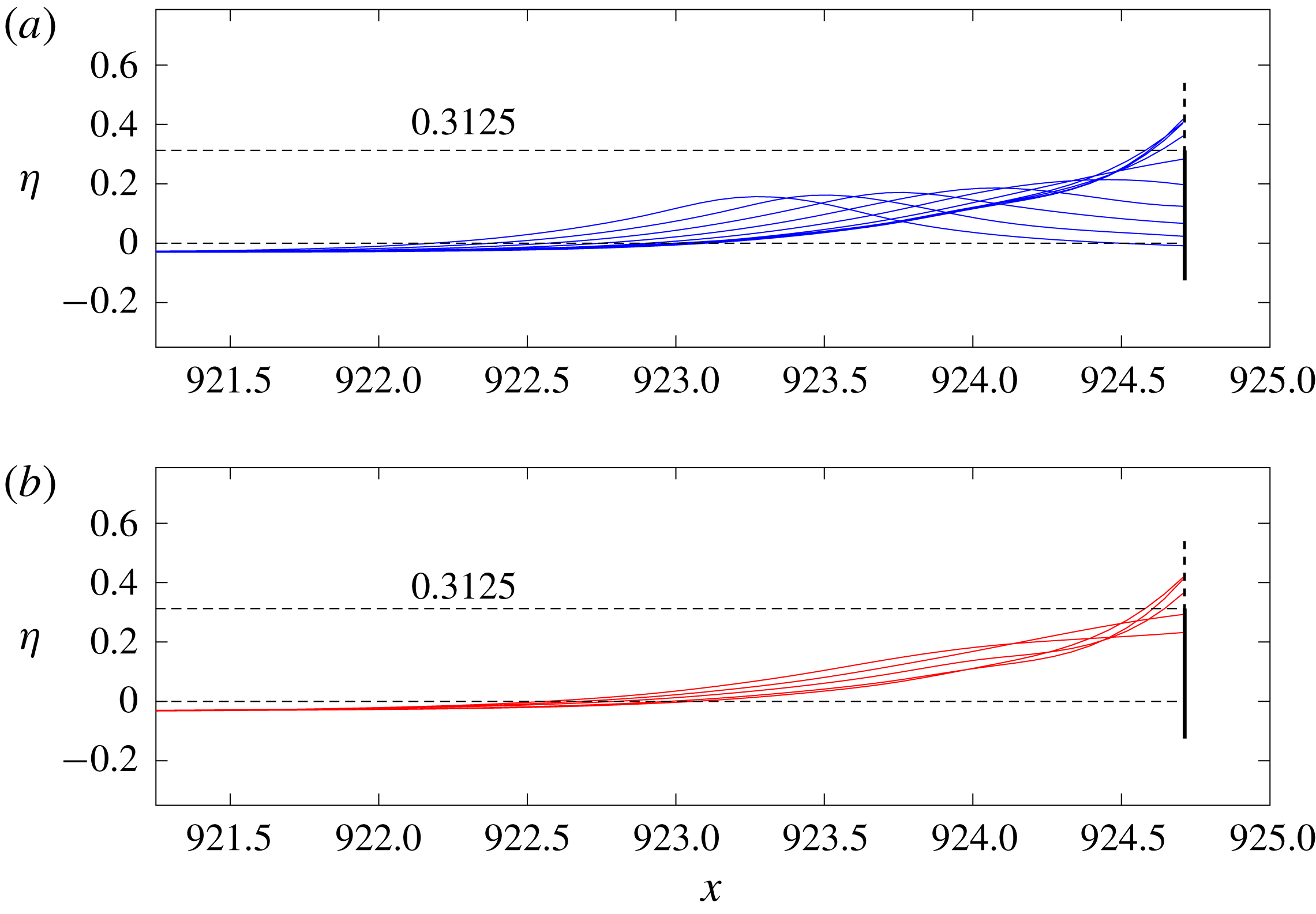
, over the Aran Islands bathymetry. The third wave (with greatest amplification) in the wave packet smoothly runs up and down the cliff face with no sign of a vertical jet (figure 7). The crest, when it is on the cliff face, has a half-wavelength of over 1.25 (dimensionally 100 m). Here,
 $R_{max}\approx 11.8$
. We highlight that a cliff of 25 m (marked by a solid vertical line at wall and a dashed horizontal line) would be overtopped by this wave.
Runup of a wave with initial parameters
 $P_{0}=175$
,
 $N_{w}=3$
,
 $a_{0}=0.043$
. (a) The wave runs up the cliff. (b) The wave is reflected from the cliff. The amplification is
 $R_{max}\approx 11.8$
. The wave smoothly runs up the face of the cliff, to the right. A cliff of (dimensionless height) 0.3125 (marked by a solid vertical line at the wall and a dashed horizontal line, dimensionally 25 m) would be overtopped by the wave.

We consider now the Aran Islands bathymetry (figure 2) to determine extreme waves that may occur in the near shore. We focus on the wave amplification and location when
 $H$
is large, as this is directly related to large wave heights.
In all simulations, the majority of non-breaking waves during evolution respect the generally accepted condition
 $H<0.55$
. However, many exceed this value for small time intervals (figure 3). The maximum value is
 $H\approx 0.951$
. Although not shown, there is a continuous
 $H(t)$
relationship that ascends to and descends from these (non-breaking) maximal values.
Such wave events occur briefly during wave–wall and wave–wave interactions. These waves have the largest non-breaking kinematic (
 $K>0.487$
) and steepness (
 $S>0.323$
) measures. All other non-breaking waves with
 $H<0.55$
have lower kinematic and steepness measures. Hence, these waves are amplified, steep and near breaking.
The scaled free-surface amplification
 $R_{a}=\unicode[STIX]{x1D702}/a_{0}$
at the crests tips of maximum
 $H$
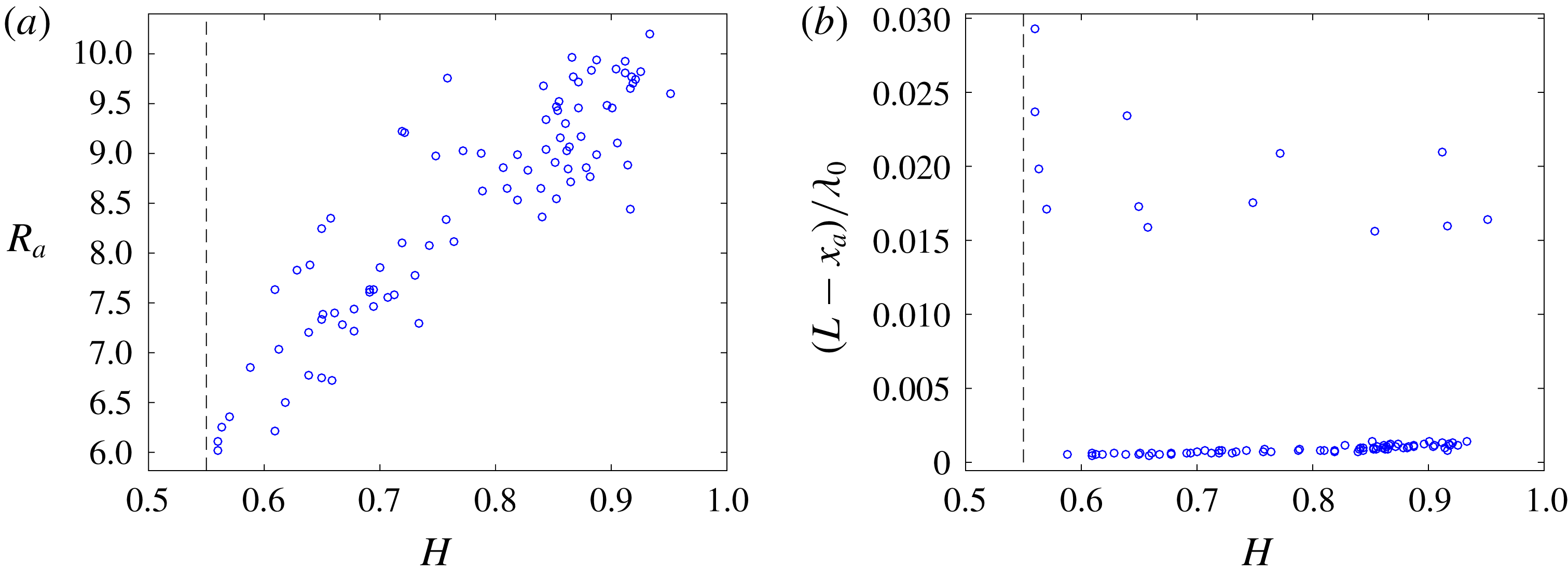
show that all waves are significantly amplified (figure 8
a);
 $R_{a}>10$
in one case and
 $R_{a}>6$
for all. In general,
 $R_{a}$
increases with
 $H$
. The location
 $x_{a}$
of these waves is evaluated as within
 $0.001\unicode[STIX]{x1D706}_{0}$
of the wall for most of the waves (figure 8
b). However, it is actually occurring on the wall face as
 ${\approx}0.001\unicode[STIX]{x1D706}_{0}$
is a small numerical error when mapping between conformal and physical space with computational domain length
 $2L=100+2(2+N_{w})\unicode[STIX]{x1D706}_{0}$
. The instances further from the wall (
 ${>}0.015\unicode[STIX]{x1D706}_{0}$
) are wave–wave interactions between an incoming and reflected waves.
We call these amplified, steep, near-breaking waves at the wall extreme waves.
Amplification and location of non-breaking crests with maximum
 $H_{w}>0.55$
. (a) Free-surface crest amplification
 $R_{a}=\unicode[STIX]{x1D702}/a_{0}$
. (b) Distance from the wall (
 $L-x_{a}$
), scaled with the initial wavelength
 $\unicode[STIX]{x1D706}_{0}$
.

4.4 Other bathymetry profiles
It has been shown how a change in bathymetry slope can affect the runup amplification: the amplification,
 $R_{max}$
, increases with slope (over the same
 $x$
distance). In this section, we consider further the effects of bathymetry.
The different piecewise-linear profiles already mentioned are not constrained by any conservation principle to give a meaningful comparison. Now we consider profiles,
 $d(x)$
, such that the area of the bathymetry is constant,
 $$\begin{eqnarray}A=\int _{0}^{L}d(x)\,\text{d}x=\text{const}.\end{eqnarray}$$
The representation taken is a Gaussian profile,
 $$\begin{eqnarray}d(x)=1-d_{L}\exp \left[-\left(\frac{x-L}{\unicode[STIX]{x1D70E}}\right)^{2}\right],\quad \unicode[STIX]{x1D70E}=\frac{2\,A}{\sqrt{\unicode[STIX]{x03C0}}\,d_{L}},\end{eqnarray}$$
where
 $d_{L}$
is the highest point of the bathymetry (at the wall,
 $x=L$
).
We initialize the wave packet in each simulation by dimensionless parameters
 $(P_{0},N_{w},a_{0})=(140,3,0.04)$
. We vary the bathymetry (4.3) via the Gaussian height (
 $d_{L}$
) and area
 $A$
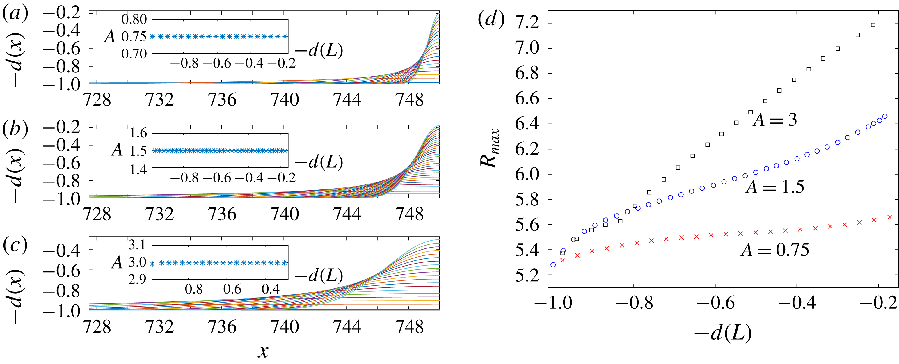
. We compare three examples with
 $A=0.75,1.5,3$
, as in figures 9(a), 9(b), 9(c) respectively. While conserving area (4.2) under the bathymetry, the maximum runup amplification increases as the Gaussian profiles change from short and wide to tall and thin, i.e. as
 $A$
increases or
 $d(L)$
decreases (figure 9
d). This means that steeper bathymetry profiles have a greater amplification effect, as expected. Furthermore, as the area taken up by the bathymetry increases, meaning the waves are affected farther out to sea or with a smaller depth, the amplification increases. Eventually, as the bathymetry steepens or
 $d(L)$
decreases (becomes shallower), wave breaking begins to occur. There is a smaller non-breaking range as
 $A$
increases.
(a–c) Bathymetries based on Gaussian profiles (4.3). In each the area (
 $A=0.75,1.5,3$
respectively) is the same but the shape differs. (d) The maximum runup amplification for each profile. The profiles are indicated by the bathymetry value at the wall,
 $-d(L)$
, for different areas
 $A=0.75$
(
 $\times$
), 1.5 (○) and 3 (▫).

5 Discussion and relevance to the real world
In this paper, we have discussed the appearance of near-shore extreme waves (steep, amplified, near breaking) at a vertical wall. The large amplification factors arise from the many (wave, wall, bathymetry) interactions in the system. It is natural to ask the question: Can these factors be a key element in describing cliff overtopping and boulder transport on platforms (Herterich, Cox & Dias Reference Herterich, Cox and Dias2018)?
The numerical values used in this paper for the incoming long waves could represent tsunamis. They could also represent infragravity waves (IGWs) or storm surges in terms of wave periods. IGWs and long storm surges are highly energetic and can magnify runup amplifications (Montoya & Lynett Reference Montoya and Lynett2018). But the wave amplitudes and the bathymetry used in the present paper are not representative of such waves. So, at this stage, we cannot conclude that the runup amplifications described in the present paper can explain natural phenomena.
Our results can contribute to a better understanding of wave breaking in the real world. Wave breaking presents a challenge to numerical modelling. Usually the wave form cannot be resolved beyond certain limits. Furthermore, we must ensure that the breakdown is not a bug in the code, but is actually a physical process such as whitecapping (breakdown of the free surface) or overturning (multifunction). Our physical assumptions in modelling the Euler equations do not capture complex air–sea interactions. Previously, the occurrence of wave breaking in this code was considered with respect to wave steepness (Viotti et al. Reference Viotti, Dutykh, Dudley and Dias2013, Reference Viotti, Carbone and Dias2014a ). We justify the occurrence of wave breaking in our simulations with reference to well-regarded and well-tested criteria based on geometric, kinematic and energetic principles. Our analysis indicates that the breakdown of simulations concurs with accepted critical values (table 2). Our simulations are performed with a potential flow model. This works very well for the onset of wave breaking (Barthelemy et al. Reference Barthelemy, Banner, Peirson, Fedele, Allis and Dias2018). Beyond breaking, computational fluid dynamics (CFD) simulations are required to resolve the flow (Derakhti et al. Reference Derakhti, Banner and Kirby2018).
As discussed, we cannot simulate wave breaking, but can observe the wave during the onset of breaking. Let us now consider the type of breaking wave that may occur in our study. In our simulations, the breaking measures (figure 3) suggest steep waves with crest tip velocities that exceed the phase velocity. On occasions, waves are considered excessive for only one of the measures. This suggests either plunging or spilling as the typical breaking wave type. Larger steepness, kinematic, energetic and breaking strength measures are associated with plunging (Perlin et al. Reference Perlin, Choi and Tian2013; Derakhti et al. Reference Derakhti, Banner and Kirby2018). The breaking strength of waves is related to the rate of change of normalized energy flux (2.14). Waves initialized with high amplitudes have the greatest breaking strengths (figure 4 b).
The influence of the bathymetry is explored with a few examples. Specifically, a representation of the Aran Islands, Ireland is considered, along with variations thereof. Tidal differences highlight the effect of depth and bathymetry variation. While a varying bathymetry affects runup amplification, it further depends on the absolute depth that governs the system. Low tides, while possessing a lower still-water free-surface elevation, are amplified by a greater amount than high tides, which possess a higher still-water level (figure 5).
Gaussian bathymetries are compared with respect to the area under the curve (figure 9). However, there are many other representative bathymetries not considered here. We can say that steepness, height, total area (displacement) of a bathymetry all contribute to increasing the runup amplification, as well as the absolute depth from the tidal effect. The bathymetry increases the runup not just far beyond linear theory, but also nonlinear results over a flat bottom.
Wave–wave interactions, a result of reflection from the wall, are key in our results and clearly affect the criteria for wave breaking. Waves are amplified by interactions with other waves in the group (figure 6), reducing the initial amplitude range for non-breaking waves (figure 3b in Herterich & Dias (Reference Herterich and Dias2017a )).
6 Conclusions
The runup of long waves at a wall can be significantly amplified by a variable bathymetry, wave–wall interactions and wave–wave interactions (figure 6), under the influence of dispersion and nonlinearity. Wave breaking is a prominent feature with a slope representing the Aran Islands bathymetry (figure 2). In particular, the nonlinear interactions of multiple waves in the wave packet reduce the maximum initial amplitude range before breaking occurs from 0.063 to 0.043 (dimensionally, 5.04 m to 3.44 m).
Wave breaking is verified with respect to several well-established criteria. The geometric (2.8), (2.9), kinematic (2.10) and energetic (2.15) breaking measures are applied to the free-surface crests in the simulations. In general there is a well-defined separation between breaking and non-breaking waves. However, there are some inconsistencies (overlapping) where non-breaking waves take breaking measures that exceed the breaking waves (figure 3). For the parameter regime in table 1, the criteria are summarized in table 2. The minimum breaking criteria obtained (
 $S=0.364$
,
 $H=0.452$
,
 $K=0.697$
and
 $B=0.871$
) are reasonably consistent for the geometric measures, and consistent for the kinematic and energetic measures (Stansell & MacFarlane Reference Stansell and MacFarlane2002; Wu & Nepf Reference Wu and Nepf2002; Perlin et al.
Reference Perlin, Choi and Tian2013; Barthelemy et al.
Reference Barthelemy, Banner, Peirson, Fedele, Allis and Dias2018).
The initial amplitude and period may influence the type of breaking. Shorter-period and higher-amplitude wave packets result in steeper waves, with larger kinematic breaking measures and breaking strengths. These are more likely to be plunging-type breaking waves, with longer periods and smaller amplitudes likely to be spilling-type breaking (Perlin et al. Reference Perlin, Choi and Tian2013; Derakhti et al. Reference Derakhti, Banner and Kirby2018).
For non-breaking waves, the maximum runup amplification increases with many parameters: initial amplitude, number of waves,
 $N_{w}$
, in the wave packet (until
 $N_{w}\geqslant 3$
where it steadies out), tidal level and slope of bathymetry (figure 5). However, the runup increases with dimensionless wave periods until up to 140, from an amplification factor of 4 to
 $9+$
(figure 5). Beyond this period, the runup continues to increase but at a lower rate. The wave smoothly runs up the wall without exhibiting a flip-through like jet (figure 7).
Tidal effects change the depth of the bathymetry by a constant change in free-surface elevation. We investigate 5 m changes in the still-water level. The runup amplification reduces by 1 with each 5 m increment (figure 5). This means that a greater depth reduces the runup amplification. The bathymetric effect is reduced with depth.
The non-breaking waves with excessive geometric and kinematic breaking measures are analysed with respect to extreme wave height-to-depth ratios. It is observed that these waves are steep, near breaking, close to the wall, with an amplification factor of 6–10.76 (figure 8). We refer to these waves as extreme near-shore waves. They smoothly run up a wall to great heights, such that they may overtop with a collapsing surge if the wall is of finite height.
Variations in bathymetry are also explored using Gaussian distributions (4.3), keeping a constant area under the profile. The runup amplification increases as the profile becomes steeper over a shorter range (figure 9). Furthermore, runup amplification increases with the area under the bathymetry curve. This is as one may expect with the bathymetry becoming a more prominent feature of the system.
The extreme amplifications obtained in this paper are for wave periods that are not typical of ocean waves. However, they can be reproduced in laboratory experiments.
Acknowledgements
Preliminary results were given in two conference papers (Herterich & Dias Reference Herterich and Dias2017a ,Reference Herterich and Dias b ) with several results included as appeared, extended or corrected. The authors thank Geological Survey Ireland and the Marine Institute for providing access to the INSS and INFOMAR datasets, and C. Viotti for his original conformal-mapping code for the Euler equations. J.G.H. would like to thank J. Brennan for helpful discussions during the preparation of this manuscript. This study was funded by Science Foundation Ireland (SFI) under the research project ‘Understanding Extreme Nearshore Wave Events through Studies of Coastal Boulder Transport’ (14/US/E3111).