



1. Introduction
Unsteady flows induced by wall-mounted bluff bodies arise in a wide range of engineering and environmental contexts across multiple scales. At larger scales, such flows are encountered in external aerodynamics around buildings (Tominaga Reference Tominaga2015; Gorlé Reference Gorlé2025), as well as in cross-flow over tube bundles in heat exchangers (Mangrulkar et al. Reference Mangrulkar, Dhoble, Chakrabarty and Wankhede2017). At smaller scales, analogous unsteady flow phenomena also arise in microfluidic devices and electronics cooling systems (Rastan et al. Reference Rastan, Sohankar and Alam2017), and in biofluid flows perturbed by arterial surface irregularities (Jia et al. Reference Jia, Punithakumar, Noga and Hemmati2021). The wall-mounted bluff body introduces an abrupt geometric disruption to the incoming flow, causing flow separation and the formation of complex vortical structures with pronounced three-dimensionality. These structures strongly affect the transport of mass, momentum and energy, making such flows important in both fundamental and applied contexts.
For flow around a wall-mounted finite-height prism, the sharp corners promote flow separation, leading to stronger vortical activity and more pronounced unsteadiness, than in the case of a smoothly contoured cylinder (Zhang et al. Reference Zhang, Li, Wang, Qiu, Fu and Liu2024). Since flow unsteadiness is commonly associated with the intensity of velocity fluctuations, its variation is closely related to the development of turbulent motions in the wake Goswami & Hemmati (Reference Goswami and Hemmati2025a
,
Reference Goswami and Hemmatib
). Accordingly, the wake dynamics of this flow configuration have remained a subject of continuing interest (Hussein & Martinuzzi Reference Hussein and Martinuzzi1996; Wang & Zhou Reference Wang and Zhou2009; Saha Reference Saha2013; Sumner et al. Reference Sumner, Rostamy, Bergstrom and Bugg2017; Wang & Lam Reference Wang and Lam2019; Goswami & Hemmati Reference Goswami and Hemmati2020, Reference Goswami and Hemmati2021, Reference Goswami and Hemmati2022, Reference Goswami and Hemmati2023, Reference Goswami and Hemmati2024, Reference Goswami and Hemmati2025a
,
Reference Goswami and Hemmatib
). The wake topology and the associated vortical structures of wall-mounted prisms are known to depend sensitively on both the flow conditions and the body geometry. Previous studies have identified important effects of the Reynolds number (Hwang & Yang Reference Hwang and Yang2004; Zhang et al. Reference Zhang, Cheng, An and Zhao2017), aspect ratio (
 $\textit{AR}$
, height-to-width ratio) (Wang et al. Reference Wang, Zhou, Chan and Lam2006; Wang & Zhou Reference Wang and Zhou2009; Saha Reference Saha2013) and depth ratio (
 $\textit{DR}$
, length-to-width ratio) (Rastan et al. Reference Rastan, Shahbazi, Sohankar, Alam and Zhou2021; Goswami & Hemmati Reference Goswami and Hemmati2022, Reference Goswami and Hemmati2024, Reference Goswami and Hemmati2025a
,
Reference Goswami and Hemmatib
). A key feature of this flow is the interaction between the free-end and wall-body-junction dynamics: the separated shear layer at the free end generates tip vortices and an induced downwash, whereas the wall-body junction gives rise to base vortices accompanied by an upwash motion (Wang et al. Reference Wang, Zhou, Chan and Lam2006; Wang & Zhou Reference Wang and Zhou2009; Sumner et al. Reference Sumner, Rostamy, Bergstrom and Bugg2017; Zhang et al. Reference Zhang, Li, Wang, Qiu, Fu and Liu2024). The wall-body junction also modifies the incoming near-wall flow. As the approaching boundary layer wraps around the prism base, a horseshoe vortex (HsV) system forms upstream of the body (Simpson Reference Simpson2001; Zhang et al. Reference Zhang, Li, Wang, Qiu, Fu and Liu2024).
Previous studies have demonstrated that, for wall-mounted finite prisms, variations in Reynolds number primarily affect the wake dynamics rather than its fundamental topological organisation. The principal coherent structures, including the HsV, the tip and base vortices, and the midspan shedding phenomena, are generally preserved across a wide range of Reynolds numbers (Saha et al. Reference Saha, Muralidhar and Biswas2000; Zhang et al. Reference Zhang, Cheng, An and Zhao2017). By contrast, vortex shedding exhibits a stronger sensitivity to Reynolds number and body geometry, and is progressively weakened and eventually suppressed as either the Reynolds number or the aspect ratio decreases (Saha Reference Saha2013; Zargar et al. Reference Zargar, Tarokh and Hemmati2021b
; Goswami & Hemmati Reference Goswami and Hemmati2022). For sufficiently large aspect ratios, coherent vortical structures are shed from the prism side shear layers and develop into C-type vortices, reverse C-type vortices and hairpin vortices (HV) (Wang & Zhou Reference Wang and Zhou2009; Dousset & Pothérat Reference Dousset and Pothérat2010; Saha Reference Saha2013; Zhang et al. Reference Zhang, Cheng, An and Zhao2017, Reference Zhang, Li, Wang, Qiu, Fu and Liu2024). It is worth noting that, during their initial formation in the near wake, these HV are lifted in the spanwise direction rather than in the vertical direction, thereby clearly distinguishing them from the HV commonly observed in turbulent boundary layers (Pan et al. Reference Pan, Wang, Zhang and Feng2008; Dennis & Nickels Reference Dennis and Nickels2011a
,
Reference Dennis and Nickelsb
; Wang et al. Reference Wang, Gao, Wang, Wang and Pan2019; Li et al. Reference Li, Wang, Qiu, Wu, Zhou, Fu and Liu2022a
, Reference Li, Wang, Qiu, Zhou, Fu and Liu2024b
). Furthermore, in cross-section, the alternating shedding of these structures from the side shear layers gives rise to a Kármán-like vortex-street pattern, accompanied by a pronounced spanwise flapping motion (Zhang et al. Reference Zhang, Li, Wang, Qiu, Fu and Liu2024). However, as the aspect ratio decreases (
 $\textit{AR}$
< 2), the periodic shedding of the side structures is suppressed by the downwash, leading to the disappearance of the Kármán-like vortex street (Sakamoto & Arie Reference Sakamoto and Arie1983). In this regime, the spanwise base and tip vortices become intrinsically connected, forming an arch-shape vortex. As it convects downstream, the arch-shape vortex gradually assumes a hairpin-like form before being transported into the wake. Hwang & Yang (Reference Hwang and Yang2004), Yakhot et al. (Reference Yakhot, Liu and Nikitin2006) and Diaz-Daniel et al. (Reference Diaz-Daniel, Laizet and Vassilicos2017) suggested that the formation of such HV originates from the destabilisation of the shear layer separated from the leading-edge of the prism top surface. Notably, the evolution of an arch-shape vortex into a hairpin vortex is not unique to flow around a wall-mounted prism, but has also been observed in the flow around a wall-mounted hemisphere (Carr & Plesniak Reference Carr and Plesniak2016; Ye et al. Reference Ye, Schrijer and Scarano2016; Tu et al. Reference Tu, Wang, Gao, She, Wang, Wang and Wei2023; Liu et al. Reference Liu, Wang, Zhu and Pan2024, Reference Liu, Zhu and Wang2025).
The depth ratio also exerts a significant influence on the global aerodynamic behaviour of wall-mounted prisms. Mashhadi et al. (Reference Mashhadi, Sohankar and Alam2021) reported that increasing the depth ratio leads to reductions in both the shedding Strouhal number (
 $\textit{St}_0$
) and the drag coefficient. Meanwhile, Kindree et al. (Reference Kindree, Shahroodi and Martinuzzi2018) and Morton et al. (Reference Morton, Martinuzzi, Kindree, Shahroodi and Saeedi2018) showed that the near wake supports instability processes over both low- and high-frequency ranges, with the latter associated with harmonic components of the primary shedding frequency. An important effect of increasing depth ratio is the promotion of shear-layer reattachment on the prism top surface after separation from the leading-edge corners (Joubert et al. Reference Joubert, Harms and Venter2015; Wang & Lam Reference Wang and Lam2019; Rastan et al. Reference Rastan, Shahbazi, Sohankar, Alam and Zhou2021). This behaviour is qualitatively similar to that observed for an infinite-span rectangular cylinder (Cimarelli et al. Reference Cimarelli, Leonforte and Angeli2018; Chiarini et al. Reference Chiarini, Gatti, Cimarelli and Quadrio2022a
,
Reference Chiarini, Quadrio and Auterib
,
Reference Chiarini, Quadrio and Auteric
; Chiarini & Auteri Reference Chiarini and Auteri2023; Cimarelli et al. Reference Cimarelli, Corsini and Stalio2024; Li et al. Reference Li, Wang, Qiu, Zhou, Fu and Liu2024a
,
Reference Li, Wang, Qiu, Zhou, Fu and Liub
). For a wall-mounted finite prism, however, the influence of depth ratio extends further. For prisms with
 $\textit{AR}=7$
, depth ratios from
 $1$
to
 $4$
, and
 $\textit{Re}_b=1.2\times 10^4$
, with
 $\textit{Re}_b$
based on the spanwise width of the prism, Rastan et al. (Reference Rastan, Shahbazi, Sohankar, Alam and Zhou2021) showed that, once the depth ratio exceeds
 $3$
, the separated flow can also reattach to the side surfaces. This behaviour is attributed to the progressive weakening of the downwash with increasing depth ratio, accompanied by an intensification of the upwash, until the downwash disappears completely at
 $\textit{DR}=3$
. The effect of depth ratio differs in low-aspect-ratio prisms. For
 $\textit{AR}=1.2$
, Zargar et al. (Reference Zargar, Tarokh and Hemmati2021b
) showed that, over the low-Reynolds-number range
 $\textit{Re}_h=50 {\sim} 250$
, with
 $\textit{Re}_h$
based on the height of the prism, increasing the depth ratio progressively weakens the upwash while strengthening the downwash. As a result, upwash remains dominant on the symmetry plane, whereas the regions near the prism side and rear faces are characterised by downwash due to the arch-shape vortex. Recently, a further consequence of depth-ratio variation was reported by Goswami & Hemmati (Reference Goswami and Hemmati2022) for wall-mounted prisms with
 $\textit{AR}=1$
. Based on numerical simulations over
 $\textit{DR}=0.016{\sim} 4$
and
 $\textit{Re}_b=50{\sim} 500$
, they showed that depth ratio affects both the onset of wake unsteadiness and the symmetry of the resulting wake. Using the limiting case of a very thin prism (
 $\textit{DR}=0.016$
) to elucidate the roles of free-end effects and side-shear-layer dynamics, they found that the wake first becomes unsteady at
 $\textit{Re}_b=200$
, while a distinct asymmetric mode emerges at
 $\textit{Re}_b=250$
. This asymmetric state is characterised by alternating shear-layer peel-off from either side of the prism, tilted HV and secondary streamwise vortices, and is attributed to out-of-phase shedding of the side shear layers and tip vortices at
 $\textit{St}_{0}/2$
. As the depth ratio increases, the shedding process becomes progressively more symmetric, the wake symmetry is restored, and the corresponding threshold depth ratio increases with Reynolds number. At a fixed large depth ratio, Zargar et al. (Reference Zargar, Tarokh and Hemmati2022b
) examined the wake transition of a wall-mounted prism with
 $\textit{DR}=5$
and
 $\textit{AR}=1.2$
over
 $\textit{Re}_h=250{\sim} 1200$
. They showed that increasing Reynolds number changes the relative importance of upwash and downwash in the mean flow, together with the size, dominant frequency and interactions of the coherent structures. Accordingly, the wake is classified into three regimes: steady for
 $\textit{Re}_h \leqslant 625$
; regular unsteady for
 $625\lt \textit{Re}_h\lt 750$
; irregular unsteady for
 $\textit{Re}_h \geqslant 750$
. Unsteadiness first appears at
 $\textit{Re}_h=625{\sim} 650$
, and a more irregular wake topology emerges by
 $\textit{Re}_h=750$
. The transition is attributed to instabilities of the separated leading-edge shear layers and their interaction with the HsV system.
The reattachment of the leading-edge shear layers promoted by increasing depth ratio enhances the interaction between large- and small-scale motions in the flow. Consequently, the effect of depth ratio on the turbulent characteristics of wall-mounted prism wakes has attracted growing attention in recent years (Goswami & Hemmati Reference Goswami and Hemmati2024, Reference Goswami and Hemmati2025a
,
Reference Goswami and Hemmatib
). After separating from the leading-edges, the shear layers can become unstable and evolve into HV, in a manner similar to that reported for infinite-span rectangular cylinders (Cimarelli et al. Reference Cimarelli, Leonforte and Angeli2018, Reference Cimarelli, Corsini and Stalio2024; Li et al. Reference Li, Wang, Qiu, Zhou, Fu and Liu2024a
,
Reference Li, Wang, Qiu, Zhou, Fu and Liub
, Reference Li, Wang, Qiu, Zhou, Fu and Liu2025a
). In particular, the Kelvin–Helmholtz (KH) instability of the separated shear layer is associated with the periodic shedding of corotating vortical structures, accompanied by low-frequency shear-layer flapping and a periodic expansion and contraction of the primary recirculation region. The resulting spanwise vortex rollers then undergo secondary instabilities, eventually developing into HV. Recent work by Goswami & Hemmati (Reference Goswami and Hemmati2024) showed that, for wall-mounted prisms with small aspect ratios (
 $\textit{AR}=0.2 {\sim} 1.5$
), increasing depth ratio over
 $\textit{DR}=1 {\sim} 4$
at
 $\textit{Re}_b=1000 {\sim} 2500$
promotes the development of KH rollers from the leading-edge shear layers, strengthens the associated high-frequency motions, and enhances their interaction with downstream HV, thereby producing a more complex wake. Their analysis further indicated that the top-surface shear layer is a primary source of pressure fluctuations, while the interaction between KH rollers and coherent wake structures provides an additional contribution. The dominant frequency of the pressure fluctuations was found to coincide with that of the KH rollers, highlighting the key role of KH instability in the downstream wake dynamics. Building on this, Goswami & Hemmati (Reference Goswami and Hemmati2025b
) further showed, over
 $\textit{AR}=0.25 {\sim} 1.5$
,
 $\textit{DR}=1 {\sim} 4$
and
 $\textit{Re}_b=1\times 10^3 {\sim} 5\times 10^3$
, that increasing depth ratio strengthens wake unsteadiness and promotes the transition towards turbulence. Their analysis of the turbulence–mean-shear interaction and turbulence–turbulence interaction terms in the Poisson equation indicated that the former is associated with energy transfer from the mean shear to the unsteady shear-layer motion near the leading-edge, whereas the latter reflects nonlinear coupling between KH rollers and large-scale vortex shedding over the prism surfaces. Further extending this line of work, Goswami & Hemmati (Reference Goswami and Hemmati2025a
) investigated the destabilisation of the leading-edge shear layer and the onset of KH instability at higher Reynolds numbers for
 $\textit{AR}=0.25 {\sim} 1.5$
,
 $\textit{DR}=1 {\sim} 4$
and
 $\textit{Re}_b=2.5\times 10^3 {\sim} 1\times 10^4$
. They found that increasing depth ratio enhances wake unsteadiness and shifts the onset of KH instability upstream, particularly for longer prisms, bringing shear-layer roll-up closer to the leading-edge. More importantly, they identified a feedback mechanism involving the secondary recirculation region, in which vortex interaction, reconnection and upstream energy convection act together to destabilise the leading-edge shear layer. Turbulence kinetic energy analysis indicated that this process is sustained by energy generation in both the primary and secondary recirculations. A related feedback mechanism has also been reported for an infinite-span rectangular cylinder, but there it is associated with the primary recirculation (Li et al. Reference Li, Wang, Qiu, Zhou, Fu and Liu2024b
).
The wake of wall-mounted finite prisms is also sensitive to the incidence angle (
 $\alpha$
). Previous studies showed that increasing
 $\alpha$
can strengthen the near-wake downwash and substantially alter shear-layer reattachment and trailing-edge interaction, thereby modifying the wake structure (Castro & Robins Reference Castro and Robins1977; Norberg Reference Norberg1993; Zargar et al. Reference Zargar, Gungor, Tarokh and Hemmati2021a
). For a large-depth-ratio prism, Zargar et al. (Reference Zargar, Goswami and Hemmati2022a
) considered the limiting case of an extreme incidence angle by examining a wall-mounted rectangular prism with
 $\textit{DR}=4.17$
at
 $\alpha =90^\circ$
and
 $\textit{Re}_h=250$
. They found that the wake topology differs markedly from that at smaller incidence angles, with the mean flow characterised by two downwash-inducing vortices and a persistent base vortex. The unsteady wake is dominated by the periodic shedding of arch-shape structures, whose legs form the base vortices and whose evolution gives rise to secondary structures between successive shedding events. The dominant unsteady frequency was reported as
 $\textit{St}_0=0.087$
, associated with these largest coherent structures. From a geometric viewpoint, the
 $\alpha =90^\circ$
configuration is also interpreted as the
 $\alpha =0^\circ$
case of a prism with an effectively small aspect ratio (
 $\textit{AR}\lt 1$
), highlighting the close connection between incidence-angle and geometry effects in wall-mounted-prism wakes. Despite these advances, several aspects of wall-mounted-prism wakes remain insufficiently understood. In particular, the influence of depth-ratio variation on wake vortex dynamics at an incidence angle of
 $90^\circ$
has received limited attention. Yet this limiting configuration is also relevant, from a geometric perspective, to the
 $\alpha =0^\circ$
case of a prism with sufficiently small aspect ratio. Clarifying how depth-ratio variation affects the wake in this setting is therefore closely connected to understanding the role of aspect-ratio reduction at zero incidence. This issue provides an important motivation for the present study.
In the present work, we investigate the vortex dynamics of flow around a wall-mounted prism at
 $\alpha =0^\circ$
, focusing on configurations with sufficiently small aspect ratios. Attention is focused on the generation and subsequent evolution of vortical structures shed from the prism, together with those developing from the HsV system, and on the associated flow mechanisms from the perspective of turbulent transport. Rather than restricting the analysis to the spanwise centre plane, as is common in the existing literature, we consider the fully three-dimensional (3-D) flow field in order to provide a more complete picture of the wake vortical dynamics. The effects of Reynolds number and spanwise extension on wake development are of particular interest. This study is expected to deepen the physical understanding of vortex dynamics and the role of spanwise extension, thereby providing further insight into the flow physics around wall-mounted bluff bodies, particularly those with sharp edges. The paper is organised as follows: § 2 describes the physical model and numerical methods; § 3 presents and discusses the main findings; § 4 summarises the conclusions.
2. Numerical methodology
2.1. Flow configuration and numerical method
In the present study, 3-D direct numerical simulations (DNS) are carried out to investigate the flow around a wall-mounted prism with varying spanwise extent. A schematic of the configuration is shown in figure 1
 $(a)$
, where
 $l$
,
 $h$
and
 $b$
denote the streamwise, vertical and spanwise dimensions of the prism mounted on the bottom wall of the computational domain, respectively. Since the present study focuses on the effect of spanwise extension on the vortex dynamics, the prism height
 $h$
is adopted as the characteristic length scale. It should be noted that, this choice differs from that in previous studies of depth-ratio effects, such as Goswami & Hemmati (Reference Goswami and Hemmati2022, Reference Goswami and Hemmati2024, Reference Goswami and Hemmati2025a
,
Reference Goswami and Hemmatib
), where the prism spanwise width was used as the characteristic scale. Accordingly, the Reynolds number is defined as
 $\textit{Re}_h={U_{\infty }h}/{\nu }$
, where
 $U_{\infty }$
is the bulk velocity and
 $\nu$
is the kinematic viscosity. Following Saha (Reference Saha2013), Zargar et al. (Reference Zargar, Tarokh and Hemmati2022b
) and Goswami & Hemmati (Reference Goswami and Hemmati2022, Reference Goswami and Hemmati2024, Reference Goswami and Hemmati2025a
,
Reference Goswami and Hemmatib
), the computational domain extends over
 $-10h \leqslant x \leqslant 22h$
in the streamwise direction,
 $0 \leqslant y \leqslant 6h$
in the vertical direction, and
 $0 \leqslant z \leqslant b+14h$
in the spanwise direction. In the present work, the streamwise scale of prism is fixed at
 $l=h$
. Three spanwise extents are considered, namely
 $b/h=1$
,
 $3$
and
 $5$
, corresponding to
 $\textit{AR}=1$
,
 $1/3$
and
 $1/5$
, respectively. For each configuration, simulations are performed at
 $\textit{Re}_h=300$
,
 $500$
and
 $1000$
. The governing equations are the dimensionless continuity and incompressible Navier–Stokes equations, written as
 \begin{equation} \boldsymbol{\nabla }\boldsymbol{\cdot }\boldsymbol{u}=0, \end{equation}
 \begin{equation} \frac {\partial \boldsymbol{u}}{\partial t}+\boldsymbol{u}\boldsymbol{\cdot }\bigtriangledown \boldsymbol{u}=-\boldsymbol{\nabla }\!p+\frac {1}{\textit{Re}_h}\boldsymbol{\nabla} ^{2}\boldsymbol{u}, \end{equation}
where
 $\boldsymbol{u}\equiv (u,v,w)$
denotes the velocity vector,
 $t$
is time and
 $p$
is pressure. Equations (2.1) and (2.2) are solved using the unsteady incompressible Navier–Stokes solver implemented in the open-source code OpenFOAM (Jasak et al. Reference Jasak, Jemcov and Tukovic2007), which has been employed in several previous studies of flow around wall-mounted prisms (Zargar et al. Reference Zargar, Tarokh and Hemmati2022b
; Goswami & Hemmati Reference Goswami and Hemmati2022, Reference Goswami and Hemmati2024; Zhang et al. Reference Zhang, Li, Wang, Qiu, Fu and Liu2024; Goswami & Hemmati Reference Goswami and Hemmati2025a
,
Reference Goswami and Hemmatib
).
 $(a)$
Schematic of the flow configuration around a wall-mounted prism, where
 $l$
,
 $h$
and
 $b$
represent the streamwise, vertical and spanwise dimensions of the prism, respectively.
 $(b,c)$
Partial views of the computational mesh for the case
 $b/h=5$
at
 $\textit{Re}_h=1000$
, shown in the
 $x$
–
 $y$
plane at
 $z/h=0$
in
 $(b)$
and in the
 $x$
–
 $z$
plane at
 $y/h=0.5$
in
 $(c)$
.

A uniform inflow condition is prescribed at the inlet, i.e.
 $u=U_{\infty }$
and
 $v=w=0$
, while a zero-normal-gradient condition,
 $\partial \boldsymbol{u}/\partial n=0$
, is imposed at the outlet. The upper and lateral boundaries of the computational domain are treated as free-slip, whereas no-slip conditions are applied on both the ground and the prism surfaces. For each case, the time step is selected such that the maximum Courant–Friedrichs–Lewy number remains below
 $0.7$
. The non-dimensional time steps adopted for the simulations at
 $\textit{Re}_h=300$
,
 $500$
and
 $1000$
are
 $0.005$
,
 $0.0075$
and
 $0.001$
, respectively. The governing equations are discretised using second-order-accurate schemes in both space and time. At each time step, convergence is assumed when the root-mean-square residual of the momentum equations falls below
 $10^{-6}$
(Zargar et al. Reference Zargar, Tarokh and Hemmati2022b
). Time integration is carried out using a second-order implicit backward scheme. Both the convective and diffusive terms are discretised using second-order central differences, and the resulting equations are solved using the pressure-implicit with splitting of operators algorithm (Goswami & Hemmati Reference Goswami and Hemmati2022, Reference Goswami and Hemmati2024). The mesh for the case
 $b/h=5$
at
 $\textit{Re}_h=1000$
is shown as a representative example in figure 1
 $(b,c)$
. Following Zargar et al. (Reference Zargar, Tarokh and Hemmati2022b
), the incoming boundary-layer properties are evaluated in the presence of the prism at
 $x/h=0$
and
 $z/h=6+b/2$
, as summarised in table 1. The quantities
 $\delta$
,
 $\delta ^*$
and
 $\theta$
denote the boundary-layer thickness, displacement thickness and momentum thickness, respectively, and the momentum-thickness Reynolds number is defined as
 $\textit{Re}_\theta =\textit{Re}_h\theta /h$
. The mesh distribution in the spanwise centre plane (
 $z/h=0$
) is presented in figure 1
 $(b)$
, while figure 1
 $(c)$
shows the mesh in the vertical plane at the prism midheight, i.e.
 $y/h=0.5$
. These views illustrate the local mesh refinement adopted near the prism surfaces, the ground wall and the immediate wake region, where large velocity gradients and strong vortical activity are expected. Such refinement is introduced to ensure adequate resolution of the near-wall flow, the separated shear layers and the subsequent wake evolution.
Incoming boundary-layer properties evaluated at
 $x/h=0$
and
 $z/h=6+b/2$
in the presence of the prism: boundary-layer thickness
 $\delta$
, displacement thickness
 $\delta ^*$
, momentum thickness
 $\theta$
and momentum-thickness Reynolds number
 $\textit{Re}_\theta =\textit{Re}_h\theta /h$
.

Table 1. Long description
A table with four columns and three rows. The columns are labeled Reh, δ/h, δ*/h, θ/h, and Reθ. The rows present values for different Reynolds numbers. Row 1: Reh, 300; δ/h, 0.86; δ*/h, 0.29; θ/h, 0.11; Reθ, 33. Row 2: Reh, 500; δ/h, 0.69; δ*/h, 0.23; θ/h, 0.09; Reθ, 45. Row 3: Reh, 1000; δ/h, 0.51; δ*/h, 0.17; θ/h, 0.07; Reθ, 70.
The simulations are first advanced for 300 non-dimensional time units to allow the flow to reach a statistically stationary state. Three-dimensional instantaneous flow fields are then stored every 0.25 non-dimensional time units, with 1200 snapshots retained for each case. The same sampling interval and number of snapshots are used for the power spectral density (PSD) and dynamic mode decomposition (DMD) analyses. As shown in § 3, several characteristic frequencies, including harmonic and subharmonic components, are identified in the present flows. The maximum and minimum numbers of periods associated with these frequencies are approximately 208 and 32, respectively, indicating that the sampling duration covers a sufficient number of periods. In addition, the frequency separation between the identified multimodal features is at least six times the frequency resolution, which supports reliable modal separation and reduces the possibility of spectral overlap or leakage between neighbouring modes. The mean flow and Reynolds-stress fields are accumulated at every time step after the statistically stationary state has been reached.
2.2. Validation and mesh sensitivity study
To assess the numerical accuracy, a mesh-sensitivity study is performed for the
 $b/h=5$
,
 $\textit{Re}_h=1000$
case. This case is expected to impose the most stringent resolution requirement among the present simulations, since it combines the highest Reynolds number with the largest spanwise extent and exhibits strong 3-D wake development, complex HsV dynamics and energetic separated shear layers. The mesh convergence is first evaluated by examining the mean drag coefficient
 $\overline {C_D}$
and the mean lift coefficient
 $\overline {C_L}$
. Four successively refined meshes are considered, containing
 $1.72\times 10^7$
,
 $2.80\times 10^7$
,
 $3.37\times 10^7$
and
 $3.83\times 10^7$
cells, respectively. The corresponding results are summarised in table 2. The differences in
 $\overline {C_D}$
and
 $\overline {C_L}$
between mesh 3 and mesh 4 are found to be only
 $0.10\,\%$
and
 $0.16\,\%$
, respectively. In addition, the mean velocity components, including the streamwise, vertical and spanwise velocities, together with the Reynolds normal stresses, are compared at several locations in both the
 $z/h=0$
and
 $y/h=0.5$
planes, as shown in figure 2. Excellent agreement is observed between mesh 3 and mesh 4 for both the first- and second-order statistics, further confirming the convergence of the spatial resolution. Therefore, mesh 3 is adopted for the subsequent simulations, as it provides grid-converged predictions of the integral force coefficients and selected first- and second-order statistical profiles. As an additional assessment of the spatial resolution, the ratio between the local mesh size and the Kolmogorov length scale,
 $\varDelta /\eta$
, is also examined (Zargar et al. Reference Zargar, Tarokh and Hemmati2022b
; Goswami & Hemmati Reference Goswami and Hemmati2022; Li et al. Reference Li, Wang, Qiu, Zhou, Fu and Liu2025a
). Here,
 $\varDelta$
is defined as the maximum cell dimension among the three coordinate directions, i.e.
 $\varDelta = \mathrm{max}({\Delta x, \mathrm{\Delta } y, \mathrm{\Delta } z})/h$
, while the Kolmogorov length scale is evaluated from
 $\eta = (\nu ^3/\varepsilon )^{1/4}$
, where
 $\varepsilon$
denotes the local dissipation rate. Previous DNS studies have shown that, in order to resolve the dissipation associated with the smallest turbulent motions, the mesh spacing should remain of the same order as the Kolmogorov scale, namely
 $\varDelta /\eta =O(1)$
(Moser & Moin Reference Moser and Moin1987; Zhou et al. Reference Zhou, Nagata, Sakai, Ito and Hayase2015; Zhou et al. Reference Zhou, Nagata, Sakai and Watanabe2019; Mahmoodi-Jezeh & Wang Reference Mahmoodi-Jezeh and Wang2020). The distribution of
 $\varDelta /\eta$
for the representative
 $b/h=5$
,
 $\textit{Re}_h=1000$
case is shown in figure 3. It is found that
 $\varDelta /\eta$
remains generally below
 $3$
throughout the flow domain, indicating that the mesh resolution is appropriate for resolving the smallest dynamically relevant scales in the present DNS. To further assess the resolution in regions most relevant to the vortex dynamics, representative mesh-resolution measures are extracted from the near-wall region, the separated shear-layer region and the HsV region, as summarised in table 3. Here,
 $\Delta _{\textit{min}}/h$
denotes the first off-wall grid spacing adjacent to the lower wall and prism surface. In all three regions, the maximum value of
 $\varDelta /\eta$
remains below approximately
 $2.3$
. This provides further confidence that the dynamically important near-wall, shear-layer and HsV motions are adequately resolved by the present mesh. The present resolution is comparable to the resolution reported by Zargar et al. (Reference Zargar, Tarokh and Hemmati2022b
), who obtained
 $\varDelta /\eta \lt 4.5$
in their DNS of flow past a streamwise-extending wall-attached prism at
 $\textit{Re}_h=1200$
. The consistency with this closely related flow configuration provides further support for the adequacy of the present mesh resolution.
Mesh sensitivity study for
 $b/h=5$
at
 $\textit{Re}_h=1000$
, based on the mean drag coefficient
 $\overline {C_D}$
and lift coefficient
 $\overline {C_L}$
. Relative errors are evaluated with respect to mesh 4.

Table 2. Long description
A table with four rows and six columns comparing mesh sensitivity study results. Columns are labeled Study, N_total, C_D bar, |ΔC_D| (%), C_L bar, and |ΔC_L| (%). Row 1: Mesh 1, 1.72, 0.996, 1.78, 0.667, 3.57. Row 2: Mesh 2, 2.80, 1.011, 0.30, 0.649, 0.78. Row 3: Mesh 3, 3.37, 1.013, 0.10, 0.645, 0.16. Row 4: Mesh 4, 3.83, 1.014, —, 0.644, —.
Mesh-resolution assessment based on the mean velocity and Reynolds-stress distributions at selected locations for the
 $b/h=5$
,
 $\textit{Re}_h=1000$
case.
 $(a,c)$
Centre plane (
 $z/h=0$
);
 $(b,d)$
prism midheight plane (
 $y/h=0.5$
).
 $(a)$
Vertical distributions of the mean streamwise and vertical velocities,
 $U$
and
 $V$
;
 $(b)$
Spanwise distributions of the mean streamwise and spanwise velocities,
 $U$
and
 $W$
;
 $(c,d)$
Vertical and spanwise distributions of the Reynolds normal stresses, respectively. Here (i)
 $x/h=1$
; (ii)
 $x/h=3$
; (iii)
 $x/h=7$
.

Representative mesh-resolution measures in dynamically important regions for the
 $b/h=5$
,
 $\textit{Re}_h=1000$
case. All lengths are normalised by the prism height
 $h$
.

Table 3. Long description
A table comparing mesh-resolution measures in dynamically important regions for a specific case. The table has four rows and five columns. The columns are labeled Region, Range, (Δxmax, Δymax, Δzmax)/h, Δmin/h, and (Δ/η)max. The rows are labeled Near-wall region, Separated shear layer, and Horseshoe-vortex region. Each row provides specific ranges and values for the respective regions. The Near-wall region has ranges -10 ≤ x/h ≤ 15, 0 ≤ y/h ≤ 0.3, and -6.5 ≤ z/h ≤ 6.5, with values (0.020, 0.077, 0.091), 0.0024, and 2.17. The Separated shear layer has ranges -0.5 ≤ x/h ≤ 3, 1 ≤ y/h ≤ 2, and -3 ≤ z/h ≤ 3, with values (0.027, 0.043, 0.026), 0.0025, and 2.30. The Horseshoe-vortex region has ranges -3 ≤ x/h ≤ -0.5, 0 ≤ y/h ≤ 0.8, and -4.5 ≤ z/h ≤ 4.5, with values (0.041, 0.020, 0.048), 0.0024, and 2.05.
Distribution of the ratio between the local mesh size and the Kolmogorov length scale,
 $\varDelta /\eta$
, for the case
 $b/h=5$
and
 $\textit{Re}_h=1000$
.
 $(a)$
Spanwise centre plane (
 $z/h=0$
);
 $(b)$
vertical plane at midheight of the prism (
 $y/h=0.5$
).

The capability of OpenFOAM in simulating flow around wall-mounted prisms has been demonstrated in previous studies (Zargar et al. Reference Zargar, Tarokh and Hemmati2022b
; Goswami & Hemmati Reference Goswami and Hemmati2022, Reference Goswami and Hemmati2024; Zhang et al. Reference Zhang, Li, Wang, Qiu, Fu and Liu2024; Goswami & Hemmati Reference Goswami and Hemmati2025a
,
Reference Goswami and Hemmatib
). Nevertheless, an additional validation step is introduced for the present numerical set-up, as the wake characteristics of an extending wall-mounted prism remain largely unexplored in the existing literature, particularly at
 $\textit{Re}_b=1000$
. As a validation case, the flow around a wall-mounted prism with
 $\textit{AR}=4$
(
 $h/b=4$
) at
 $\textit{Re}_h=1000$
is considered, and the resulting mean velocity profiles are compared in figure 4 with the DNS data of Zhang et al. (Reference Zhang, Cheng, An and Zhao2017). The comparison includes the three mean velocity components, namely the streamwise, vertical and spanwise velocities, at selected locations, and good agreement is obtained for all components. In addition, the present mean drag coefficient is
 $\overline {C_D}=1.417$
, close to the reference value of
 $1.404$
, while the Strouhal number based on the prism spanwise width is
 $\textit{St}_b=0.107$
, compared with
 $0.106$
in Zhang et al. (Reference Zhang, Cheng, An and Zhao2017). The relative differences in both quantities are less than
 $1\,\%$
, further supporting the accuracy of the present numerical method.
Comparison of mean velocity profiles between the present results and the DNS of Zhang et al. (Reference Zhang, Cheng, An and Zhao2017) for a wall-mounted prism with
 $\textit{AR}=4$
(
 $h/b=4$
) at
 $\textit{Re}_b=1000$
.
 $(a$
–
 $c)$
Mean streamwise velocity profiles at
 $x/b=3$
for
 $(a) \,y/b=1$
,
 $(b)\, y/b=2$
and
 $(c)\, y/b=3$
.
 $(d$
–
 $f)$
Mean velocity profiles at
 $x/b=7$
and
 $y/b=3$
:
 $(d)$
streamwise,
 $(e)$
vertical and
 $(f)$
spanwise components.

3. Results and discussion
3.1. Instantaneous 3-D vortices and mean flow field
This section begins with a visualisation of the instantaneous vortical structures. It then examines the effects of spanwise extension and Reynolds number on the mean-flow statistics, focusing in particular on the mean-flow topology and the characteristic scales of the separation bubbles. These results provide an overall description of vortex generation and evolution, and serve as a basis for the subsequent investigation of wake vortex dynamics in § 3.2. Table 4 presents the main vortical structures discussed in the present study.
3.1.1. Instantaneous 3-D vortices
The instantaneous 3-D vortical structures are identified using the
 $Q$
-criterion with
 $Q=0.1$
. Figure 5
 $(a$
–
 $c)$
present the corresponding instantaneous wake structures at
 $\textit{Re}_h=300$
for the three prisms with different spanwise widths, namely
 $b/h=1$
,
 $3$
and
 $5$
. At this low Reynolds number, the wake retains a relatively regular vortical organisation. In addition, although the flow field is instantaneous, the vortex distribution is nearly symmetric about the centre plane with
 $z/h=0$
, consistent with previous observations for prism wakes at low Reynolds numbers under
 $\textit{DR}$
variation (Goswami & Hemmati Reference Goswami and Hemmati2022). Nonetheless, variations in
 $b/h$
exert a clear influence on the wake organisation. For
 $b/h=1$
, as shown in figure 5
 $(a)$
, separated shear layers form from the prism leading-edge, but no evident shear-layer instability develops and the wake remains nearly steady. Even when a smaller isosurface level,
 $Q=0.025$
, is used, no distinct vortical structures are observed farther downstream. For
 $b/h=3$
, by contrast, the separated shear layer undergoes a clear KH instability, as shown in figure 5
 $(b)$
, leading to the formation of KH vortex. The KH vortex subsequently evolves into arch-shaped vortices (ArcV) in the near wake, which then develop further into primary HV farther downstream. As
 $b/h$
is increased further to
 $5$
, as shown in figure 5
 $(c)$
, the wake becomes noticeably broader owing to the larger spanwise extent of the prism. The overall wake organisation remains broadly similar to that at
 $b/h=3$
. However, ArcV now undergoes a secondary instability and becomes progressively distorted as it evolves downstream. This observation is reminiscent of the rapid onset of spanwise instability in the vortex rollers after their separation from the upper and lower shear layers in the flow around a near-wall circular cylinder with infinite span (Li et al. Reference Li, Wang, Qiu, Wu, Zhou, Fu and Liu2022a
,
Reference Li, Wang, Qiu, Wu, Zhou, Fu and Liub
). It is worth noting that, at
 $\textit{Re}_h=300$
, the present spanwise-extended prism flow already exhibits unsteady vortex shedding. This behaviour contrasts with the streamwise-extended prism with
 $\textit{DR}=5$
studied by Zargar et al. (Reference Zargar, Tarokh and Hemmati2022b
), for which the flow remained steady up to
 $\textit{Re}_h=625$
. This comparison suggests that the spanwise-extended configuration exhibits an earlier transition towards unsteady wake dynamics than the streamwise-extended counterpart under the corresponding conditions. Zargar et al. (Reference Zargar, Tarokh and Hemmati2022b
) also reported a different route to HV formation for a streamwise-extended prism. At
 $\textit{Re}_h=650$
, HVs form over the upper surface and, owing to the large streamwise length of the prism, convect downstream along the surface before separating again from the trailing edge and entering the wake. In contrast, the side-edge shear layers remain stable and do not generate HVs until
 $\textit{Re}_h$
is increased to
 $675$
, when periodic shedding from the side edges is observed. This behaviour differs markedly from the present spanwise-extended prism flow. In the present
 $\textit{Re}_h=300$
cases, HV formation originates from the upper shear layer only, and the HVs develop after the separated flow leaves the prism.
 $(a$
–
 $c)$
Instantaneous 3-D vortical structures at
 $\textit{Re}_h=300$
, visualised by the isosurface
 $Q=0.1$
and coloured by the instantaneous streamwise velocity
 $u/U_{\infty }$
. The grey isosurface in
 $(a)$
corresponds to
 $Q=0.025$
.
 $(d$
–
 $f)$
Close-up views of the HsV system. Panels (a)–(c) show top views of the vortical structures within the regions delineated by the white boxes in
 $(a{-}c)$
, respectively. Panels (d)–(f) show the corresponding cross-sectional views in the plane
 $z/h=0$
. For
 $x/h\lt -0.5$
, the vortices are coloured by spanwise vorticity
 $\omega _z$
(red, positive; blue, negative), whereas for
 $x/h\gt -0.5$
, they are coloured by streamwise vorticity
 $\omega _x$
(orange, positive; purple, negative). The primary and secondary horseshoe vortices are labelled, while higher-order vortices are indicated by magenta arrows. Here
 $(a,d)\, b/h=1$
;
 $(b,e)\, b/h=3$
;
 $(c,f)\, b/h=5$
. Unless otherwise specified, the colour scale for streamwise velocity in the subsequent figures is identical to that adopted here.

In addition, a HsV system is formed around the prism in all three flows, as shown in the close-up top views in figure 5
 $(d$
–
 $f)$
. These panels correspond to the vortical structures within the regions delineated by the white boxes in figure 5
 $(a$
–
 $c)$
, respectively. The primary HsV, characterised by negative spanwise vorticity (
 $\omega _z$
), rolls up immediately upstream the prism. Its formation is primarily associated with the impingement of the incoming boundary layer on the prism and the ensuing separation induced by the adverse pressure gradient, as illustrated in figure 6. The HsV subsequently wraps around the front junction and is reoriented into a streamwise vortex with negative streamwise vorticity (
 $\omega _x$
). As shown in figure 5
 $(d)$
, for
 $b/h=1$
, the HsV further induces a secondary HsV (SHsV) with positive
 $\omega _z$
. After reorientation, the SHsV develops into a streamwise vortex with positive
 $\omega _x$
, forming a counter-rotating vortex pair with the HsV. From the centre-plane view, the SHsV is seen to be much smaller than the HsV and is located upstream of and below it. For
 $b/h=3$
, as shown in figure 5
 $(e)$
, the combined induction of the HsV and SHsV gives rise to a higher-order HsV, which is likewise characterised predominantly by negative
 $\omega _z$
. This higher-order vortex is located upstream of the SHsV and at a higher vertical position. However, its strength weakens substantially during the reorientation process, preventing any further development into a streamwise vortex. Similar features have also been reported in flow around a wall-mounted hemisphere (Liu et al. Reference Liu, Wang, Zhu and Pan2024, Reference Liu, Zhu and Wang2025). When
 $b/h$
is increased to
 $5$
, however, the HsV system becomes simplified again, as shown in figure 5
 $(f)$
. In this case, the SHsV no longer appears immediately in front of the prism, but instead emerges near the reorientation region, where it successfully develops into a streamwise vortex. This behaviour is associated with the different local pressure-gradient distributions upstream of the prism, as shown in figure 6. The SHsV and HsV are located on the upstream and downstream sides of the adverse-pressure-gradient region, respectively. For
 $b/h=5$
, the adverse pressure gradient immediately upstream of the prism (indicated by the arrow) is considerably weaker than those for
 $b/h=1$
and
 $b/h=3$
, as shown in figure 6
 $(a$
–
 $c)$
. Such a weakened adverse pressure gradient suppresses the local separation required for the formation of the SHsV in front of the prism. As the vortex system extends in the spanwise direction, however, the adverse pressure gradient becomes substantially enhanced near the reorientation region, providing favourable conditions for the emergence of the SHsV there. At the present Reynolds number of
 $\textit{Re}_h=300$
, the HsV system stays steady in all three flows, both upstream of the prism and along its sides.
Instantaneous distributions of the streamwise pressure gradient at
 $y/h=0.3$
for
 $\textit{Re}_h=300$
:
 $(a) \,b/h=1$
,
 $(b)\, b/h=3$
and
 $(c)\, b/h=5$
.

When the Reynolds number is increased to
 $\textit{Re}_h=500$
, the wake structures exhibit a more intricate 3-D organisation than those at
 $\textit{Re}_h=300$
, as shown in figure 7. This change is evident not only from the richer vortical structures, but also from the enhanced turbulent fluctuations discussed in § 3.3. For
 $b/h=1$
, in particular, the flow is no longer steady, as illustrated in figure 7
 $(a)$
. The HV evolving from the ArcV subsequently emerge as the dominant wake structures. As shown in figures 7
 $(a)$
and 7
 $(d)$
, the HsV system also becomes richer than that at
 $\textit{Re}_h=300$
, with a higher-order HsV of negative
 $\omega _z$
generated under the combined induction of the HsV and SHsV. However, after reorientation, this higher-order HsV decays rapidly, and only the HsV and SHsV persist as a counter-rotating vortex pair extending downstream. After lifting away from the wall, these two vortices give rise to side HV (SHV). As noted above, such SHV are commonly observed in flows around wall-mounted bluff bodies (Goswami & Hemmati Reference Goswami and Hemmati2022, Reference Goswami and Hemmati2025a
,
Reference Goswami and Hemmatib
; Liu et al. Reference Liu, Wang, Zhu and Pan2024; Zhang et al. Reference Zhang, Li, Wang, Qiu, Fu and Liu2024; Liu et al. Reference Liu, Zhu and Wang2025). For
 $b/h=3$
, as shown in figures 7
 $(b)$
and 7
 $(e)$
, both the HsV and the higher-order HsV rapidly weaken after reorientation, in the sense that their apparent strength and spatial coherence decrease under the same vortex-identification threshold. These structures then disappear shortly downstream of the reorientation region, whereas only the SHsV remains coherent and extends farther downstream in the streamwise direction. The absence of the HsV after reorientation suppresses the formation of SHV. The ArcV also undergoes secondary instability, as in the
 $\textit{Re}_h=300$
,
 $b/h=5$
case. During flow downstream evolution, the SHsV deflects towards the centre plane and eventually disappears after interacting with the HV evolved from the ArcV. For
 $b/h=5$
, as shown in figures 7
 $(c)$
and 7
 $(f)$
, the HsV system on the windward side of the prism no longer contains a higher-order vortex with positive
 $\omega _z$
, and is therefore more similar to that for
 $b/h=1$
than to that for
 $b/h=3$
. However, both the HsV and SHsV are able to extend downstream after reorientation, thereby enabling the formation of SHV. Moreover, at the present spanwise width, the HV evolved from the ArcV undergo a more pronounced upward lift around
 $x/h= 14$
than in the
 $b/h=3$
case. This non-monotonic behaviour can be attributed to the geometry-induced redistribution of the 3-D pressure-gradient field around the prism, which modifies the separation characteristics and the evolution of the HsV system. The corresponding instantaneous pressure-gradient distributions are shown in figure 8. In the reorientation region, the strong adverse pressure gradient for
 $b/h=3$
extends only to
 $x/h\approx -0.47$
(figure 8
 $b$
), close to the streamwise location of the prism leading edge. By contrast, for
 $b/h=1$
and
 $5$
, the adverse-pressure-gradient region extends farther downstream, reaching
 $x/h\approx -0.23$
and
 $0.06$
, respectively. This indicates that the adverse pressure gradient along the prism side persists over a longer streamwise distance in these two cases. Consequently, during the reorientation process, the flow for
 $b/h=1$
and
 $5$
(figures 8
 $a$
and 8
 $c$
) remains subjected to an adverse pressure gradient, which helps sustain flow separation and supports the persistence of the HsV. For
 $b/h=3$
, however, the shorter streamwise extent of the adverse-pressure-gradient region is less effective in maintaining the separated flow, leading to rapid weakening and eventual disappearance of the HsV. Similarly, in the present
 $\textit{Re}_h=500$
case, the HVs still originate from the upper shear layer and form only after the separated flow leaves the prism, consistent with the behaviour observed at
 $\textit{Re}_h=300$
. This indicates that, even at
 $\textit{Re}_h=500$
, the route to HV formation remains fundamentally different from that reported for the streamwise-extended wall-mounted prism by Zargar et al. (Reference Zargar, Tarokh and Hemmati2022b
).
 $(a$
–
 $c)$
Instantaneous 3-D vortical structures at
 $\textit{Re}_h=500$
, visualised by the isosurface
 $Q=0.1$
and coloured by the instantaneous streamwise velocity
 $u/U_{\infty }$
.
 $(d$
–
 $f)$
Close-up views of the HsV system, presented in the same format as in figure 5, including the colouring scheme and vortex annotations. Here (a,d)
 $b/h=1$
; (b,e)
 $b/h=3$
; (c, f)
 $b/h=5$
.

Instantaneous distributions of the streamwise pressure gradient at
 $y/h=0.3$
for
 $\textit{Re}_h=500$
:
 $(a) b/h=1$
,
 $(b) b/h=3$
and
 $(c) b/h=5$
.

When the Reynolds number is further increased to
 $\textit{Re}_h=1000$
, the wake is characterised by more fragmented vortical structures, stronger spanwise undulations and enhanced three-dimensionality, as shown in figure 9. The corresponding increase in turbulent activity is further supported by the statistics presented in § 3.3. For
 $b/h=1$
, as illustrated in figures 9
 $(a)$
and 9
 $(c)$
, the number of higher-order horseshoe vortices upstream of the prism increases substantially. Moreover, SHV form farther upstream than at lower Reynolds numbers. In the present case, SHV already appears upstream of
 $x/h=3$
, whereas at
 $\textit{Re}_h=500$
(figure 7
a) it emerges only downstream of
 $x/h=3$
. Interestingly, a dual-row of SHV is identified farther downstream. For
 $b/h=3$
and
 $5$
, as shown in figure 9(b–f), the two flows exhibit broadly similar behaviour. In both cases, the upstream HsV system becomes unstable, and strong interactions develop among the multiorder horseshoe vortices, giving rise to braid vortices that develop in the streamwise direction. These braid vortices convect across the leading-edge corner of the prism. Their passage introduces local disturbances near the leading-edge shear layer and is accompanied by earlier shear-layer destabilisation and subsequent vortex shedding. Meanwhile, the unstable HsV system generates SHV at an early stage of reorientation, introducing disturbances that propagate downstream along the prism sides and trigger rapid shedding from the side shear layers. As the wake develops, the SHV and HV interact strongly to form a complex turbulent wake, within which the centrally located HV undergo rapid upward lift under the strong background shear. The instability of the HsV system is a notable finding. It was not reported in previous studies of wall-mounted prisms at
 $\textit{Re}_b=1\times 10^3 {\sim} 5\times 10^3$
with smaller spanwise extent, where the influence of
 $\textit{DR}$
was the primary focus (Goswami & Hemmati Reference Goswami and Hemmati2025a
,
Reference Goswami and Hemmatib
). This behaviour is nevertheless reminiscent of the fragmented HsV system reported by Cao & Tamura (Reference Cao and Tamura2020) for flow around a wall-mounted hemisphere at
 $\textit{Re}_D=7\times 10^4 {\sim} 7\times 10^5$
. A notable difference, however, is that no braid vortices were observed to form and pass over the hemisphere in that high-Reynolds-number flow. A possible explanation is that, under such conditions, the thinner incoming boundary layer places the HsV system much lower relative to the hemisphere height.
 $(a$
–
 $c)$
Instantaneous 3-D vortical structures at
 $\textit{Re}_h=1000$
, visualised by the isosurface
 $Q=0.1$
and coloured by the instantaneous streamwise velocity
 $u/U_{\infty }$
.
 $(d$
–
 $f)$
Close-up views of the HsV system, presented in the same format as in figure 5, including the colouring scheme and vortex annotations. Here (a,d)
 $b/h=1$
; (b,e)
 $b/h=3$
; (c, f)
 $b/h=5$
.

3.1.2. Mean flow characteristics
Figure 10 shows the vertical-integrated mean pressure coefficient on the windward face of the prism for
 $\textit{Re}_h=1000$
. For
 $b/h=1$
, a pronounced centreline peak indicates a concentrated stagnation-pressure region near the midspan. However, the short spanwise length allows the end flow and lateral leakage to affect almost the entire span, limiting the development of a spanwise-extended HsV system. For
 $b/h=3$
and
 $5$
, the pressure distribution exhibits a centreline depression with two off-centre maxima, indicating a spanwise redistribution of the upstream pressure buildup. This spanwise-modulated pressure field promotes 3-D flow redistribution and makes the HsV system more susceptible to spanwise deformation. This susceptibility is further related to the incoming boundary-layer state listed in table 1. With increasing
 $\textit{Re}_h$
, the increase in
 $\textit{Re}_\theta$
reflects stronger inertial effects and weaker viscous damping in the incoming boundary layer. Consequently, the separated shear layer induced by the adverse pressure gradient becomes more susceptible to disturbance amplification, consistent with the transition from relatively steady horseshoe vortices at lower
 $\textit{Re}_h$
to unstable, braid-vortex-producing dynamics at
 $\textit{Re}_h=1000$
.
Spanwise distribution of the vertically integrated mean pressure coefficient on the windward face of the prism for
 $\textit{Re}_h=1000$
.

In contrast to near-wall infinitely long rectangular cylinders reported in the literature (Li et al. Reference Li, Wang, Qiu, Zhou, Fu and Liu2025a
,
Reference Li, Wang, Qiu, Zhou, Fu and Liub
), the wake of the present wall-mounted prism exhibits enhanced complexity, arising from spanwise geometric non-uniformity and the resulting 3-D effects. The flow separates at the leading-edge corners and subsequently reattaches downstream, giving rise to a pronounced recirculation over and behind the prism. Figure 11
 $(a)$
quantifies the spanwise variation of the mean downstream recirculation size
 $A/h^2$
, defined as the streamwise extent of the mean reverse-flow region downstream of the prism leading edge. Overall,
 $A/h^2$
decreases with increasing spanwise distance from the centre plane, although a slight local enlargement is observed near the spanwise locations corresponding to the prism side edges. For
 $b/h=1$
,
 $A/h^2$
is generally larger at higher
 $\textit{Re}_h$
, while the three Reynolds number cases exhibit broadly similar spanwise distributions, as shown in figure 11(a i). For
 $b/h=3$
and
 $5$
, however, the opposite Reynolds number dependence is observed in an overall sense:
 $A/h^2$
tends to decrease as
 $\textit{Re}_h$
increases, although local deviations occur near the side-edge regions, as shown in figures 11(a ii) and 11(a iii), respectively.
 $(a)$
Spanwise variation of the mean recirculation size
 $A/h^2$
, defined as the streamwise extent of the mean reverse-flow region downstream of the prism leading edge: (i)
 $b/h=1$
; (ii)
 $b/h=3$
; (iii)
 $b/h=5$
. The insets show enlarged views of the local peaks. The grey dashed lines denote the side-edge positions of the prism.
 $(b,c)$
Mean vertical velocity at
 $z/h=0.3$
, overlaid with contours of negative streamwise velocity to delineate the recirculation: (b)
 $b/h=1$
; (c)
 $b/h=5$
. Here (i)
 $\textit{Re}_h=300$
; (ii)
 $\textit{Re}_h=500$
; (iii)
 $\textit{Re}_h=1000$
. In
 $(b)$
, the arrow marks the strong upwash above the prism; in
 $(c)$
, it marks the transition from the upwash above the prism to the downstream downwash.

The opposite trends of the recirculation size with increasing
 $\textit{Re}_h$
for different
 $b/h$
cases are related to the corresponding changes in the upwash and downwash motions. As reported by Goswami & Hemmati (Reference Goswami and Hemmati2023), these motions play an important role in determining the extent of the recirculation region. Figures 11
 $(b)$
and 11
 $(c)$
show the mean vertical velocity in the
 $z$
–
 $y$
plane for
 $b/h=1$
and
 $5$
, respectively, at different
 $\textit{Re}_h$
, in order to elucidate the corresponding variations in upwash and downwash. Contours of negative mean streamwise velocity are superimposed to delineate the recirculations. Since the behaviour for
 $b/h=3$
is similar to that for
 $b/h=5$
, only the latter is presented here. For
 $b/h=1$
, the flow separating from the leading-edge corners is closely associated with the upwash that originates upstream of the prism and extends over it. As
 $\textit{Re}_h$
increases, the region of strong upwash expands farther downstream. This strengthens the separation at the leading-edge corners and, in turn, enlarges the recirculation over the prism. Although the upwash near
 $x/h= 2$
in the near-wall region becomes stronger from
 $\textit{Re}_h=300$
(figure 11
b i) to
 $\textit{Re}_h=500$
(figure 11
b ii), and locally suppresses the recirculation, the overall recirculation is nevertheless larger at
 $\textit{Re}_h=500$
owing to the much stronger leading-edge separation. At
 $\textit{Re}_h=1000$
(figure 11
b iii), the near-wall upwash region becomes smaller, leading to a further increase in the near-wall recirculation compared with
 $\textit{Re}_h=500$
, while the recirculation over the prism also intensifies. Together, these effects produce the largest recirculation at
 $\textit{Re}_h=1000$
. For
 $b/h=5$
, as shown in figure 11
 $(c)$
, the reduction in recirculation with increasing
 $\textit{Re}_h$
is mainly associated with a decrease in its streamwise extent. This behaviour is primarily attributed to the upstream shift of the transition location from upwash over the prism to downwash as
 $\textit{Re}_h$
increases. As a result, the flow is deflected towards the wall and reattaches earlier, leading to a smaller recirculation. By contrast, for
 $b/h=1$
, the location of this upwash-to-downwash transition varies little with
 $\textit{Re}_h$
, and the streamwise extent of the recirculation therefore remains largely unchanged.
Moreover, the different degrees of collapse in figure 11
 $(a)$
reflect the competition between the geometry-controlled side-edge flow and the Reynolds number dependent midspan wake dynamics. For
 $b/h=1$
, the prism has a very short spanwise length, with the side edge located at
 $z/h=b/(2h)=0.5$
. The end flow, lateral leakage and reoriented HsV therefore influence almost the entire span. As a result, the spanwise distribution of the downstream recirculation is primarily constrained by the short-span geometry, leading to the approximate collapse of the three Reynolds number cases in figure 11(a i). For larger spanwise lengths, the midspan wake becomes more distinct from the side-edge region, while the side-edge flow still affects a substantial portion of the span. The recirculation size is therefore governed by both the Reynolds number dependent wake recovery and the geometry-induced side-edge flow. This combined effect prevents a clear collapse for
 $b/h=3$
, as shown in figure 11(a ii). For
 $b/h=5$
, however, the
 $\textit{Re}_h=300$
and
 $500$
cases still exhibit an approximate collapse, whereas the
 $\textit{Re}_h=1000$
case departs from this trend, as shown in figure 11(a iii). The similarity between the
 $\textit{Re}_h=300$
and
 $500$
cases for
 $b/h=5$
suggests that their downstream recirculation is regulated by a similar wake-evolution process. As will be discussed in § 3.2, these cases share comparable ArcV-to-HV evolution patterns, including the formation of smaller HVs, which tends to fragment the large-scale wake structure and thereby limits the development of an enlarged recirculation region.
Figure 12 presents the 3-D mean recirculation regions for the three
 $b/h$
cases at
 $\textit{Re}_h=500$
, which are chosen as representative examples. At elevations comparable to the prism height, the downstream recirculation extends over a large portion of the prism span. At lower elevations, however, the recirculation isosurface becomes increasingly indented in the spanwise direction, indicating a reduction in the spanwise extent of the reverse-flow region. This 3-D contraction accounts for the overall decrease in
 $A/h^2$
with increasing distance from the centre plane in figure 11
 $(a)$
. The small local peaks near the spanwise locations corresponding to the prism side edges can also be understood from figure 12. Separation from the prism side edges generates local reverse-flow regions along the lateral sides of the prism. These side-edge recirculation regions extend downstream and locally increase the streamwise extent of the mean reverse-flow region, thereby producing the small peaks in the spanwise distribution of
 $A/h^2$
. For
 $b/h=1$
(figure 12
a i), a small isolated recirculation is observed within approximately
 $2.52\lt x/h\lt 4.90$
and
 $0.96\lt z/h\lt 1.23$
, as marked by the magenta arrow. This region is separated from the main recirculation behind the prism and is responsible for the additional local peak at
 $z/h\approx 1.05$
in figure 11(a i). The corresponding
 $z$
–
 $y$
plane shows a distinct pair of mean streamwise vortices above this small recirculation, associated with the reoriented HsV–SHsV pair. The lifting of this counter-rotating vortex pair promotes the formation of the SHV head, beneath which a persistent low-streamwise-velocity region develops. Since the SHV is generated in a quasisteady manner at
 $\textit{Re}_h=500$
, this low-velocity region is maintained in the mean field and gives rise to the isolated recirculation. This Reynolds number dependence is associated with the formation and stability of the SHV. At
 $\textit{Re}_h=300$
, the SHV is not formed, so that the corresponding SHV-induced local recirculation is absent. At
 $\textit{Re}_h=1000$
, the stronger HV–SHV interaction and enhanced 3-D mixing inhibit the persistence of a stable local recirculation. Consequently, no additional local peak is observed at either
 $\textit{Re}_h=300$
or
 $1000$
in figure 11
 $(a)$
. For
 $b/h=5$
(figure 12
a iii), a similar recirculation extension appears within approximately
 $3.66\lt x/h\lt 7.11$
and
 $2.01\lt z/h\lt 3.20$
. Unlike the
 $b/h=1$
case, however, this region remains connected to the main recirculation and is located close to the prism side edge. This is also indicated by the isosurface colour, which denotes the spanwise position: the small recirculation for
 $b/h=5$
has a colour level close to that of the side-edge recirculation, whereas that for
 $b/h=1$
is clearly separated from the side-edge region. Consequently, in the spanwise quantification of the recirculation size, the recirculation extension for
 $b/h=5$
is incorporated into the side-edge recirculation rather than appearing as a separate peak. This accounts for the larger side-edge peak at
 $\textit{Re}_h=500$
compared with those at
 $\textit{Re}_h=300$
and
 $1000$
in figure 11(a iii). By contrast, for
 $b/h=3$
(figure 12
a ii), only a weak outward protrusion of the recirculation is observed over approximately
 $2.60\lt x/h\lt 4.61$
. This protrusion remains attached to the main recirculation and is too weak to produce either an isolated local peak in
 $A/h^2$
, as in the
 $b/h=1$
case, or a pronounced enhancement of the side-edge peak, as in the
 $b/h=5$
case. Therefore, the
 $\textit{Re}_h=500$
,
 $b/h=3$
curve in figure 11(a ii) does not show a comparable local increase in
 $A/h^2$
.
 $(a)$
Three-dimensional spatial distribution of the recirculation at
 $\textit{Re}_h=500$
, represented by the isosurface of zero mean streamwise velocity and coloured by the spanwise coordinate
 $z/h$
. Contours in the
 $x$
–
 $z$
plane denote the mean streamwise velocity. Here (i)
 $b/h=1$
; (ii)
 $b/h=3$
; (iii)
 $b/h=5$
. The yellow curve near the prism indicates the locus of the local maximum streamwise velocity. Green arrows mark high-velocity regions, while black arrow indicates low-velocity region between adjacent high-velocity regions. Magenta arrow marks the recirculation associated with the SHV. In (i), a
 $z$
–
 $y$
plane above this recirculation is shown, where the mean streamwise vortices are coloured by
 $\omega _x$
(orange, positive; purple, negative).
 $(b)$
Mean vertical velocity at
 $x/h=0.5$
, overlaid with vortices coloured by
 $\omega _x$
(orange, positive; purple, negative) at
 $\textit{Re}_h=500$
. Here (i)
 $b/h=1$
; (ii)
 $b/h=3$
; (iii)
 $b/h=5$
.
 $(c)$
Quantities evaluated along the locus of local maximum streamwise velocity indicated by the yellow curve in
 $(a)$
: (i) mean streamwise pressure gradient; (ii) mean spanwise pressure gradient; (iii) mean streamwise velocity.

Figure 12
 $(a)$
also shows the mean streamwise velocity in the
 $x$
–
 $z$
plane. A high-streamwise-velocity region (indicated by green arrows) extending from the prism side leading-edge is evident, corresponding to the acceleration induced by flow separation. This region is flanked by a low-streamwise-velocity zone (black arrows), which is in turn bounded by another high-streamwise-velocity region (green arrows). Such a pattern is particularly pronounced for
 $b/h=5$
(figure 12
a iii). A similar feature has been reported in flow around a wall-mounted hemisphere (Liu et al. Reference Liu, Zhu and Wang2025). This behaviour arises from the exchange between high- and low-velocity fluid driven jointly by the upwash and downwash induced by the counter-rotating streamwise vortex pair, originating from the reoriented HsV and SHsV, and by the legs of the HV developing from the side shear layers (Liu et al. Reference Liu, Zhu and Wang2025). A comparison of the three flows shows that, at
 $\textit{Re}_h=500$
, the high-streamwise-velocity region extending from the prism side leading-edge is smaller for
 $b/h=3$
than for
 $b/h=1$
and
 $5$
. This observation is reminiscent of consistent with the rapid decay of the HsV after reorientation in this region, as shown in figure 7
 $(b)$
. The formation of this high-streamwise-velocity region is governed by the combined effects of side shear-layer separation and the HsV. The HsV is located above the interface between this high-velocity region and the adjacent low-velocity region, such that the HsV, characterised by negative
 $\omega _x$
, transports high-velocity fluid towards the near-wall region through a downwash motion. However, as shown in figure 12(b ii), the weakened HsV for
 $b/h=3$
induces a much weaker downwash than in the
 $b/h=1$
and
 $5$
cases, shown in figures 12(b i) and 12(b iii), respectively. In addition, the pressure gradients are evaluated along the locus of local maximum streamwise velocity within the high-velocity region, indicated by the yellow curve in figure 12
 $(a)$
. The streamwise and spanwise pressure gradients are shown in figures 12(c i) and 12(c ii), respectively. For
 $b/h=3$
, the magnitudes of both local pressure gradients are the smallest among the three cases, indicating that side shear-layer separation is weakest in this configuration. The weaker side shear-layer separation, together with the reduced downwash, leads to a smaller high-streamwise-velocity region extending from the prism side leading-edge for
 $b/h=3$
, as well as the lowest local maximum streamwise velocity, as shown in figure 12(c iii). This may also help explain why the SHsV tends to migrate towards the centre plane in this case, as shown in figure 7(b).
3.2. Vortex-dynamics mechanisms
The evolution of vortex structures is a crucial aspect of vortex dynamics. Accordingly, this section examines the effects of Reynolds number and prism spanwise extent on the instantaneous vortex organisation, with particular emphasis on the flow physics associated with the different characteristic frequencies.
For the case of
 $\textit{Re}_h=300$
and
 $b/h=1$
, the flow remains steady, as shown in figure 5
 $(a)$
, and therefore does not exhibit meaningful vortex dynamical behaviour. For the unsteady cases, flow around wall-mounted prisms is generally characterised by periodic vortex shedding. To characterise the unsteady wake dynamics, velocity fluctuations are monitored at several locations in the 3-D flow field. The probes are preferentially placed in regions traversed by the dominant wake structures, so that the identified frequency components can be associated with specific vortex-dynamical processes (Zargar et al. Reference Zargar, Tarokh and Hemmati2022b
; Tu et al. Reference Tu, Wang, Gao, She, Wang, Wang and Wei2023; Liu et al. Reference Liu, Zhu and Wang2025; Goswami & Hemmati Reference Goswami and Hemmati2025b
). The dependence of the spectral features on probe location has also been examined to ensure that the reported frequencies are not artefacts of a particular sampling point. For brevity, the results discussed below are based on representative probes placed along the trajectories of the dominant vortical structures, following the approach of Zargar et al. (Reference Zargar, Tarokh and Hemmati2022b
). Owing to the strongly 3-D nature of the flow, these probes are distributed in 3-D space for some cases, rather than being confined to the centre plane. This choice also facilitates comparison between the identified spectral signatures and the topological features of the DMD modes. Since the HV represents the dominant coherent structure in the wake, the characteristic frequency associated with the HV is referred to as the dominant frequency in the present study. Here DMD (Schmid Reference Schmid2010) is employed to extract the dominant frequency modes from the flow snapshots, thereby providing a systematic description of the underlying dynamics. Previous studies have also demonstrated the effectiveness of DMD in analysing vortex dynamics (He et al. Reference He, Wang and Pan2013; Pan et al. Reference Pan, Wang, Wang and Sun2017; Li et al. Reference Li, Wang, Qiu, Wu, Zhou, Fu and Liu2022a
, Reference Li, Wang, Qiu, Zhou, Fu and Liu2024b
, Reference Li, Wang, Qiu, Zhou, Fu and Liu2025a
; Goswami & Hemmati Reference Goswami and Hemmati2025a
; Lin et al. Reference Lin, Jia and Zhong2026). In the present study, DMD is performed on 3-D flow fields, with each snapshot comprising all three velocity components. In addition, a full-rank DMD decomposition is adopted in the present analysis. The modes discussed below are selected by jointly considering the dominant frequencies identified from the PSD analysis and the corresponding global modal-energy contributions.
3.2.1. The
 $\textit{Re}_h=300$
cases

The PSDs at different spatial locations for the
 $\textit{Re}_h=300$
,
 $b/h=3$
case are shown in figure 13
 $(a)$
. The locations from
 $M_1$
to
 $M_4$
trace the evolution of the KH vortices from their initial formation to their transformation into HV and subsequent downstream convection. The dominant frequency of the present flow is
 $\textit{St}_0=0.146$
, which characterises both the KH instability of the leading-edge shear layer and the dynamics of the HV. This behaviour differs markedly from that in the flow around a near-wall infinite-span rectangular cylinder, where the KH vortices generated in the leading-edge shear layer undergo merging and subsequently form leading-edge vortices, so that the dominant frequency is distinct from the KH instability frequency and exhibits harmonic relationships (Li et al. Reference Li, Wang, Qiu, Zhou, Fu and Liu2025a
). The topology of the DMD mode at
 $\textit{St}_0$
is shown in figure 13
 $(b)$
. The mode exhibits a regular alternating pattern in the streamwise direction, confirming the periodic nature of the flow. At location
 $M_5$
, a pronounced spectral peak appears at
 $3\textit{St}_0$
. This peak is associated with a previously unreported vortex-evolution process and is therefore fundamentally different from the harmonic frequency content observed in the wake of the infinite-span rectangular cylinder (Zhang et al. Reference Zhang, Kareem, Xu and Jiang2023; Li et al. Reference Li, Wang, Qiu, Zhou, Fu and Liu2024b
, Reference Li, Wang, Qiu, Zhou, Fu and Liu2025a
). The evolution of present prism wake are illustrated in figure 13
 $(d)$
. After the formation of the ArcV, a counter-rotating HV is generated beneath it, as shown in figure 13(d i). The counter-rotating HV has also been observed in the wake of a wall-mounted hemisphere (Liu et al. Reference Liu, Wang, Zhu and Pan2024). However, the two situations differ markedly. In the present flow, the counter-rotating HV remains closely attached to the ArcV, whereas in the hemisphere wake it is located farther from the HV head, despite the two structures having nearly superposed legs. Here, the legs of the counter-rotating HV are induced by the downstream HV legs and extend in the streamwise direction. In addition, secondary vortices (SV) are generated on the inner sides of the HV legs under the induction of the downstream HV legs, with each leg inducing an SV of opposite
 $\omega _x$
. As the wake develops downstream (figure 13
d ii), the counter-rotating HV rapidly splits into two streamwise-elongated vortical structures, while the SV are substantially amplified and develop into pronounced streamwise vortices. At this stage, an accessory vortex forms near the head of the hairpin vortex. The streamwise cross-sectional view (inset) shows that the accessory vortex has the same sign of
 $\omega _x$
as the HV leg to which it is attached. Farther downstream (figure 13
d iii), the accessory vortex becomes further strengthened. The evolution of these vortical structures gives rise to three distinct velocity-fluctuation events within a single shedding period. Figure 13
 $(c)$
shows the time history of the velocity fluctuation at location
 $M_5$
, whose position is indicated by a cyan cube in figure 13(e). The instantaneous flow fields corresponding to three instants within one period are shown in figure 13
 $(e)$
. These three fluctuation events are associated with the downstream convection of the HV (
 $t=t_1$
, figure 13
e i), the accessory vortex (
 $t=t_2$
, figure 13
e ii) and the SV (
 $t=t_3$
, figure 13
e iii), respectively. This explains the appearance of the
 $3\textit{St}_0$
peak in the spectrum at location
 $M_5$
.
Frequency characteristics and vortex-dynamical behaviour for the flow at
 $\textit{Re}_h=300$
and
 $b/h=3$
.
 $(a)$
The PSDs of the streamwise velocity fluctuations at five spatial locations:
 $M_1(2,\,1.5,\,0)$
,
 $M_2(4.5,\,1.8,\,0)$
,
 $M_3(8.5,\,2.15,\,0)$
,
 $M_4(10.5,\,2.8,\,0)$
and
 $M_5(14,\,1.2,\,0.6)$
. Here,
 $\textit{St}_0=0.146$
is the characteristic frequency of the HV.
 $(b)$
Isosurfaces of the real part of the DMD mode for the streamwise component at
 $\textit{St}_0$
, with isovalues of
 $\pm 0.0006$
.
 $(c)$
Time history of the streamwise velocity fluctuation at
 $M_5$
.
 $(d)$
Evolution of the different vortices, identified by the
 $Q$
-criterion with
 $Q=0.1$
and coloured by
 $\omega _x$
. The
 $z$
–
 $y$
plane shows the distribution of vortical structures in a streamwise cross-section extracted from the 3-D vortex field, with positive and negative values indicated by
 $\omega _x$
. Here (i)
 $t=t_0$
; (ii)
 $t=t_0+\Delta t$
; (iii)
 $ t=t_0+2\Delta t$
, where
 $\Delta t=1.75$
.
 $(e)$
Instantaneous 3-D flow fields at the three instants marked in
 $(c)$
: (i)
 $t=t_1$
; (ii)
 $t=t_2$
; (iii)
 $t=t_3$
. The cyan cube indicates the location of
 $M_5$
.

For the
 $\textit{Re}_h=300$
,
 $b/h=5$
case, the frequency characteristics and vortex-dynamical behaviour are shown in figure 14(a i). The dominant frequency measured at location
 $M_1$
is
 $\textit{St}_0=0.202$
, which represents the dominant frequency of this flow. This location lies in the centre plane, and the measured frequency characterises the KH instability of the shear layer, the formation of KH vortices and their subsequent evolution into ArcV. Location
 $M_2$
is positioned off the centre plane, as indicated by the cyan cube in figure 14
 $(c)$
. The signals at
 $M_3$
to
 $M_5$
reflect the periodic fluctuations induced in the centre plane by the downstream evolution of the wake vortices. Notably, the dominant downstream frequency is
 $\textit{St}_0/2$
, rather than
 $\textit{St}_0$
. This behaviour is closely related to the distinct evolution modes of ArcV into HV. Instantaneous flow fields (figure 5
c) show that ArcV can split into two HV that are symmetrically distributed about the centre plane. To further elucidate the mechanism responsible for the
 $\textit{St}_0/2$
component, phase-averaging (Wlezien & Way Reference Wlezien and Way1979; Luo et al. Reference Luo, Fang and Ertas2009; Ostermann et al. Reference Ostermann, Woszidlo, Nayeri and Paschereit2015) is performed using the streamwise velocity fluctuation at
 $M_3$
as the phase reference. The phase-averaged streamwise velocity fluctuation at
 $M_2$
over one shedding period is shown in figure 14(a ii). Two distinct peaks are observed within one period, with corresponding phases denoted by
 $\phi _1$
and
 $\phi _2$
, consistent with the PSDs in figure 14(a i). The phase-averaged flow fields at
 $\phi _1$
and
 $\phi _2$
are shown in figures 14(c i) and 14(c ii), respectively. At phase
 $\phi _1$
, two small-scale HV, resulting from the splitting of ArcV, convect past
 $M_2$
. At phase
 $\phi _2$
, by contrast, the ArcV does not split, and a single large-scale HV passes
 $M_2$
. Thus, two distinct wake modes are present during the downstream evolution of ArcV: one consisting of two symmetric small-scale HV and the other of a single large-scale HV. These modes alternate periodically. Consequently, although a signal with
 $\textit{St}_0$
is detected at
 $M_2$
, it arises from the superposition of these two wake modes. The DMD modal structures at
 $\textit{St}_0$
and
 $\textit{St}_0/2$
are shown in figures 14(b i) and 14(b ii), respectively. Both exhibit clear periodic organisation. The
 $\textit{St}_0$
mode is primarily associated with KH vortex formation, ArcV development and the location of small-scale HV, showing good spatial coherence consistent with the instantaneous, phase-averaged and spectral results. In contrast, the
 $\textit{St}_0/2$
mode is characterised by larger-scale structures and exhibits stronger coherence near the centre plane, in agreement with the local fluctuation features revealed by the PSDs. Reconstruction of the flow field using the
 $\textit{St}_0$
and
 $\textit{St}_0/2$
modes yields the vortical structures shown in figure 14(d i). Two small-scale HV and one large-scale HV alternate in the streamwise direction, further confirming the coexistence and periodic alternation of the two wake modes. The corresponding streamwise velocity fluctuation field is shown in figure 14(d ii). The sweep motions induced by both small- and large-scale HV generate low-speed regions beneath them, while high-speed regions form between the two small-scale HV in the spanwise direction and between the two wake modes in the streamwise direction. Therefore, the
 $\textit{St}_0/2$
signal observed in the centre plane downstream arises from the periodic alternation of the two wake modes and the associated evolution of high- and low-speed structures.
Frequency characteristics and vortex-dynamical behaviour for the flow at
 $\textit{Re}_h=300$
and
 $b/h=5$
. (a i) The PSDs of the streamwise velocity fluctuations at five spatial locations:
 $M_1(2,\,1.6,\,0)$
,
 $M_2(7,\,1.8,\,1.65)$
,
 $M_3(8.8,\,1.8,\,0)$
,
 $M_4(11,\,2.6,\,0)$
and
 $M_5(14,\,2.6,\,0)$
. Here,
 $\textit{St}_0=0.202$
is the characteristic frequency of the HV. (a ii) Phase-averaged streamwise velocity fluctuation at
 $M_3$
as a function of phase. The phases of the two peaks are denoted by
 $\phi _1$
and
 $\phi _2$
.
 $(b)$
Isosurfaces of the real part of the DMD mode for the streamwise component with isovalues of
 $\pm 0.0006$
: (i)
 $\textit{St}_0$
; (ii)
 $\textit{St}_0/2$
.
 $(c)$
Phase-averaged 3-D vortices obtained using the streamwise velocity fluctuation signal at
 $M_2$
as the phase reference: (i)
 $\phi _1$
; (ii)
 $\phi _2$
. The vortices are identified by the
 $Q$
-criterion with
 $Q=0.1$
and coloured by the phase-averaged streamwise velocity. The cyan cube marks the location of
 $M_2$
.
 $(d)$
Flow field reconstructed from the DMD modes at
 $\textit{St}_0$
and
 $\textit{St}_0/2$
: (i) vortical structures identified by the
 $Q$
-criterion with
 $Q=0.1$
and coloured by instantaneous streamwise velocity; (ii) the same vortical structures shown in grey and overlaid with streamwise velocity fluctuations, where red and blue denote positive and negative values, respectively.

3.2.2. The
$\textit{Re}_h=500$
cases

For the
 $\textit{Re}_h=500$
,
 $b/h=1$
case, the frequency characteristics at different spatial locations are shown in figure 15
 $(a)$
. Since SHV are present in this flow (figure 7
a), an additional probe location (
 $M_3$
) is introduced to characterise their frequency. As seen in figure 15
 $(a)$
, the dominant frequency is
 $\textit{St}_0=0.211$
, which characterises the KH instability, the HV dynamics and the SHV. Here, SHV and HV are generated and evolve in near synchrony, exhibiting a one-to-one correspondence. The topology of the DMD mode at
 $\textit{St}_0$
is shown in figure 15
 $(b)$
. A clear periodic organisation is observed both near the centre plane, where HV form and evolve, and in the outer region associated with SHV formation and evolution. This indicates that the
 $\textit{St}_0$
mode simultaneously captures the periodic behaviour of SHV and HV. This behaviour contrasts with the wake of a wall-mounted hemisphere, where HV and SHV are associated with distinct characteristic frequencies and modes (Liu et al. Reference Liu, Zhu and Wang2025). As shown in figure 15(c i), the HV undergo lateral deflection as they convect downstream, resulting in an instantaneous asymmetric wake. Similar vortex-dynamical behaviour has been reported in wall-mounted prisms with varying
 $\textit{DR}$
(Goswami & Hemmati Reference Goswami and Hemmati2022) and in wall-mounted hemisphere flows (Liu et al. Reference Liu, Zhu and Wang2025). A close-up view is presented in figure 15(c ii). Together with streamwise cross-sectional slices and instantaneous vortex structures, it shows that the SHV originate from the reoriented HsV and SHsV. The apparent disconnection between SHV and the HsV/SHsV is partly due to the choice of
 $Q$
-isosurface level, but more importantly reflects the rapid decay of the HsV and SHsV as they extend to approximately
 $x/h= 2.5$
. Consistent with observations in wall-mounted hemisphere wakes (Liu et al. Reference Liu, Zhu and Wang2025), the SHsV rise more rapidly than the HsV during downstream evolution, resulting in the outer leg of the SHV being located higher than the inner leg and producing a slight twisting of the structure. Furthermore, SHV are initiated by the formation of vortex legs, whereas HV develop first through the formation of vortex heads, consistent with the formation mechanisms reported for wall-mounted hemisphere flows (Tu et al. Reference Tu, Wang, Gao, She, Wang, Wang and Wei2023; Liu et al. Reference Liu, Zhu and Wang2025).
Frequency characteristics and vortex-dynamical behaviour for the flow at
 $\textit{Re}_h=500$
and
 $b/h=1$
. (a i) The PSDs of the streamwise velocity fluctuations at five spatial locations:
 $M_1(1,\,1.6,\,0)$
,
 $M_2(3.45,\,1.5,\,0)$
,
 $M_3(3.4,\,0.8,\,1)$
,
 $M_4(6,\,1.7,\,0)$
and
 $M_5(10,\,2,\,0)$
. Here,
 $\textit{St}_0=0.211$
is the characteristic frequency of the HV.
 $(b)$
Isosurfaces of the real part of the DMD mode for the streamwise component at
 $\textit{St}_0$
, with isovalues of
 $\pm 0.0006$
. (c i) Instantaneous 3-D vortices identified by the
 $Q$
-criterion with
 $Q=0.1$
and coloured by the instantaneous streamwise velocity. (c ii) Close-up view of (c i), showing the formation of SHV from the reoriented SHsV. Contours on slices at different streamwise locations denote
 $\omega _x$
.

At
 $\textit{Re}_h=500$
, when the prism spanwise extent increases to
 $b/h=3$
and
 $5$
, the wake exhibits vortex-dynamical behaviour similar to that observed for the
 $\textit{Re}_h=300$
,
 $b/h=5$
case. The characteristic frequency associated with the shear-layer KH instability and the formation of ArcV acts as the dominant frequency, whereas farther downstream the wake is dominated by a subharmonic at half this value. However, as shown in figures 16
 $(a)$
and 16
 $(b)$
, two distinct characteristic frequencies,
 $\textit{St}_{01}$
and
 $\textit{St}_{02}$
, are detected in the region where ArcV form downstream of the destabilised shear layers, for both
 $b/h=3$
and
 $b/h=5$
. For
 $b/h=3$
,
 $\textit{St}_{01}=0.267$
and
 $\textit{St}_{02}=0.287$
, whereas for
 $b/h=5$
,
 $\textit{St}_{01}=0.244$
and
 $\textit{St}_{02}=0.280$
. The DMD modal structures corresponding to
 $\textit{St}_{01}$
and
 $\textit{St}_{02}$
for
 $b/h=3$
are shown in figures 16(c i) and 16(c ii). Both display a clear regular alternating pattern, indicating that they capture periodic vortex shedding. A similar feature is observed for
 $b/h=5$
, as shown in figures 16(d i) and 16(d ii). Compared with the
 $b/h=3$
case, the
 $b/h=5$
flow exhibits an additional regular alternating pattern in the outer region, consistent with the PSDs measured at location
 $M_5$
(figure 16
b). This difference arises from the presence of SHV in the
 $b/h=5$
flow, which are absent for
 $b/h=3$
. The PSD and DMD results further indicate that, for
 $b/h=5$
, the characteristic frequency of the SHV coincides with that of ArcV. In contrast to the single dominant frequency observed for the
 $\textit{Re}_h=300$
,
 $b/h=5$
case, both the
 $b/h=3$
and
 $5$
flows at
 $\textit{Re}_h=500$
exhibit two dominant frequencies, indicating the coexistence of two shedding modes. This behaviour is likely associated with the excitation of additional instabilities and the strengthening of their mutual interactions as the Reynolds number increases. The phase-averaged results for
 $b/h=3$
and
 $5$
are shown in figures 16(c iii) and 16(d iii), respectively. In both cases, the wake exhibits a similar spatial organisation, with a pair of small-scale HV located upstream of a large-scale HV. This closely resembles the wake behaviour in the
 $\textit{Re}_h=300$
,
 $b/h=5$
case, where ArcV evolve either into two spanwise-aligned small-scale HV or into a single large-scale HV, with the two wake modes occurring alternately in a periodic manner. This also explains the appearance of subharmonic peaks at
 $\textit{St}_{01}/2$
and
 $\textit{St}_{02}/2$
in the downstream PSDs (figures 16
a and 16
b), which dominate the far wake. Furthermore, for the
 $\textit{Re}_h=500$
,
 $b/h=5$
case, the phase-averaged result in figure 16(d iii) shows that SHV accompany both the small- and large-scale HV in a one-to-one manner. This further confirms that the formation of SHV is synchronised with the ArcV dynamics.
Frequency characteristics and vortex-dynamical behaviour for the flows at
 $\textit{Re}_h=500$
with
 $b/h=3$
and
 $5$
.
 $(a)$
The PSDs of the streamwise velocity fluctuations at five spatial locations for
 $b/h=3$
:
 $M_1(1.5,\,1.7,\,0)$
,
 $M_2(4,\,1.7,\,0)$
,
 $M_3(6,\,1.9,\,0)$
,
 $M_4(8,\,1.9,\,0)$
and
 $M_5(10,\,1.9,\,0)$
. Here,
 $\textit{St}_{01}=0.267$
and
 $\textit{St}_{02}=0.287$
denote the characteristic frequencies of the HV.
 $(b)$
The PSDs of the streamwise velocity fluctuations at five spatial locations for
 $b/h=5$
:
 $M_1(1.5,\,1.8,\,0)$
,
 $M_2(4,\,1.8,\,0)$
,
 $M_3(6.5,\,2,\,0)$
,
 $M_4(8.5,\,2.2,\,0)$
and
 $M_5(10,\,0.6,\,2.4)$
. Here,
 $\textit{St}_{01}=0.244$
and
 $\textit{St}_{02}=0.280$
denote the characteristic frequencies of the HV.
 $(c,d)$
Isosurfaces of the real part of the DMD mode for the streamwise component, with isovalues
 $\pm 0.0006$
, at (i)
 $\textit{St}_{01}$
and (ii)
 $\textit{St}_{02} $
, together with phase-averaged 3-D vortical structures identified with
 $Q=0.1$
and coloured by the phase-averaged streamwise velocity (iii)
 $(c) b/h=3$
;
 $(d) b/h=5$
.

3.2.3. The
$\textit{Re}_h=1000$
cases

As the Reynolds number increases to
 $\textit{Re}_h=1000$
, the vortex-dynamical behaviour in the vicinity of the prism becomes markedly more complex. For
 $b/h=1$
, the KH instability of the top and side shear layers is characterised using the PSDs at locations
 $M_1$
and
 $M_2$
in figure 17
 $(a)$
. The two shear layers exhibit distinct characteristic frequencies, with
 $\textit{St}_{01}=0.620$
associated with the top shear layer and
 $\textit{St}_{02}=0.696$
with the side shear layer. In addition, owing to the presence of a dual-row of SHV (figure 9
a), the dynamics of the inner and outer SHV are examined at locations
 $M_3$
and
 $M_4$
, respectively. As shown in figure 17
 $(a)$
, both locations are dominated by the frequency
 $\textit{St}_{02}$
, indicating that the SHV dynamics are governed by the same frequency as the KH instability of the side shear layer. The DMD modal structures corresponding to
 $\textit{St}_{01}$
and
 $\textit{St}_{02}$
are shown in figures 17(b i) and 17(b ii), respectively. The
 $\textit{St}_{01}$
mode exhibits a regular arrangement of structures extending from the top surface of the prism, reflecting the periodic vortex formation associated with the top shear layer and consistent with the PSD at
 $M_1$
. In contrast, the
 $\textit{St}_{02}$
mode is characterised by well-organised structures originating from the prism sides, while the coherence of structures developing from the top surface is comparatively weak. Moreover, the
 $\textit{St}_{02}$
mode displays two spanwise outward expansions around
 $x/h= 2$
and
 $x/h= 3$
, corresponding to the formation of the inner and outer SHV, respectively. Thus, the
 $\textit{St}_{02}$
mode captures not only the periodic KH instability of the side shear layer but also the vortex dynamics of both the inner and outer SHV. These results demonstrate that, for the
 $\textit{Re}_h=1000$
,
 $b/h=1$
case, two distinct shedding and wake modes with different characteristic frequencies coexist. This contrasts with the behaviour at lower Reynolds numbers, where the dual wake modes arise from alternative evolution pathways of the same underlying structure, namely the transition from ArcV to HV. In the present case, however, the two modes originate from distinct spatial regions and are associated with different vortex-generation mechanisms, corresponding to instabilities of the top and side shear layers, respectively. A mismatch between the shedding frequency from the top shear layer and that of the SHV has also been reported in the wake of a wall-mounted hemisphere (Liu et al. Reference Liu, Zhu and Wang2025). However, notable differences remain. In the hemisphere wake, the SHV frequency is approximately
 $3/2$
times that of the HV shed from the hemisphere (Liu et al. Reference Liu, Zhu and Wang2025), whereas in the present wall-mounted prism flow, the shedding frequency from the top shear layer and that of the SHV are relatively close and do not exhibit a clear harmonic relationship. Furthermore, the structures shed from the upper and side shear layers resemble those reported for the streamwise-extended prism at the same Reynolds number (Zargar et al. Reference Zargar, Tarokh and Hemmati2022b
). However, in the present flow, these structures are generated only after the separated flow leaves the prism, rather than developing over the prism surface. As shown in figure 17
 $(c)$
, the evolving SHV interacts with the structures from the side shear layer and suppresses their growth. Consequently, the dominant wake structures are mainly formed from the upper shear layer and the reoriented horseshoe vortices, similar to the behaviour observed for the streamwise-extended prism at the same Reynolds number (Zargar et al. Reference Zargar, Tarokh and Hemmati2022b
).
Frequency characteristics and vortex-dynamical behaviour for the flow at
 $\textit{Re}_h=1000$
and
 $b/h=1$
.
 $(a)$
The PSDs of the streamwise velocity fluctuations at five spatial locations:
 $M_1(0.9,\,1.6,\,0)$
,
 $M_2(0.5,\,0.55,\,1)$
,
 $M_3(2,\,0.6,\,1.3)$
,
 $M_4(3.1,\,0.45,\,1.75)$
,
 $M_5(6,\,1.5,\,0)$
and
 $M_6(10,\,1.5,\,0)$
. Here,
 $\textit{St}_{01}=0.620$
and
 $\textit{St}_{02}=0.696$
denote the characteristic frequencies of the HV and SHV, respectively.
 $(b)$
Isosurfaces of the real part of the DMD mode for the streamwise component, with isovalues
 $\pm 0.0006$
: (i)
 $\textit{St}_{01}$
; (ii)
 $\textit{St}_{02}$
.
 $(c)$
Two distinct KH-vortex formation modes, with instantaneous 3-D vortical structures identified by the
 $Q$
-criterion (
 $Q=0.1$
) and coloured by instantaneous streamwise velocity: (i) asynchronous instability of the top and side shear layers; (ii) synchronous instability of the top and side shear layers. The inset shows a close-up view of the dual-row SHV, coloured by instantaneous
 $\omega _x$
.
 $(d\,\mathrm{i})$
Isosurfaces of the real part of the DMD mode for the streamwise component at
 $\textit{St}_{01}/4$
, with isovalues
 $\pm 0.0006$
; (ii)–(iv) instantaneous 3-D flow field evolution viewed from the side, with vortical structures identified by the
 $Q$
-criterion (
 $Q=0.1$
) and coloured by instantaneous streamwise velocity. Here (ii)
 $t=t_0$
; (iii)
 $t=t_0+\Delta t$
; (iv)
 $t=t_0+2\Delta t$
,
 $\Delta t =3.2$
. The cyan cubes indicate the loactions of
 $M_5$
and
 $M_6$
.

Owing to the close proximity of their characteristic frequencies, the KH vortices shed from the top and side shear layers exhibit both asynchronous and synchronous shedding during the flow evolution. As shown in figure 17(c i), the KH vortices shed from the side shear layer appear earlier than those from the top shear layer, resulting in a clear phase offset and hence asynchronous shedding. By contrast, in figure 17(c ii), the KH vortices shed from the two shear layers show little phase offset, indicating synchronous shedding. In both cases, the inner SHV remain synchronised with the KH vortices from the side shear layer and form consistently around
 $x/h= 2$
. Similarly, the outer SHV are also phase-locked to the side-shear-layer KH vortices and form around
 $x/h= 3$
. These instantaneous vortex-dynamical features are fully consistent with the PSD and DMD results. Although the outer SHV are much weaker than the inner SHV, their formation process is similar, with the vortex legs forming prior to the development of the vortex head. The key difference lies in their origin. As shown in figure 17
 $(c)$
, the inner SHV originate from the reoriented and strongly paired HsV and SHsV. By contrast, in the present flow, only the higher-order HsV with positive
 $\omega _x$
persist after reorientation. Under the combined induction of this higher-order vortex and the inner SHV, a weak quasistreamwise vortex forms beneath the inner SHV and pairs with the higher-order HsV. Their subsequent lifting then gives rise to the outer SHV. In addition, a low-frequency component at
 $\textit{St}_{01}/4$
is detected at the downstream locations
 $M_5$
and
 $M_6$
(figure 17
a). The corresponding DMD mode at
 $\textit{St}_{01}/4$
(figure 17
d i) exhibits pronounced large-scale periodic structures. Similar low-frequency behaviour has also been reported in wall-mounted prism flows at higher Reynolds numbers (Goswami & Hemmati Reference Goswami and Hemmati2025a
,
Reference Goswami and Hemmatib
), although the characteristic ratios differ, being
 $1/5$
of the KH frequency for
 $\textit{DR}=1$
and
 $1/7.6$
for
 $\textit{DR}=4$
. The underlying vortex-dynamical mechanism, however, was not clarified in those studies. The present results show that this low-frequency component arises from the periodic formation and downstream convection of large-scale HV packets, as illustrated by the instantaneous evolution in figure 17(d ii–d iv). The time interval between figures 17(d ii) and 17(d iv) approximately corresponds to one period associated with
 $\textit{St}_{01}/4$
. Notably, the large-scale HV packets in these two snapshots occupy similar streamwise locations, indicating that the flow returns to a comparable phase after one period of large-scale-structure formation. Moreover, the spacing between successive vortex packets is consistent with the spatial distribution of large-scale structures of the DMD mode shown in figure 17(d i), confirming that the
 $\textit{St}_{01}/4$
component is associated with the dynamics of these large-scale HV packets. Furthermore, in light of the correspondence between vortex merging and harmonic content reported by Li et al. (Reference Li, Wang, Qiu, Zhou, Fu and Liu2025a
), the present results suggest that each large-scale HV packet is formed through the merging of four HV originating from the top shear layer within one shedding period.
For the
 $\textit{Re}_h=1000$
,
 $b/h=3$
case, the upstream HsV system becomes unstable and gives rise to braid vortices, as shown in figure 9
 $(b)$
. To characterise this behaviour, local velocity fluctuations within the HsV system are analysed, and the corresponding PSDs at locations
 $M_1$
and
 $M_2$
are presented in figure 18
 $(a)$
. Two distinct characteristic frequencies,
 $\textit{St}_{1}=0.108$
and
 $\textit{St}_{2}=0.128$
, are identified. These are close in value and do not exhibit a harmonic relationship. The DMD modal structures corresponding to
 $\textit{St}_{1}$
and
 $\textit{St}_{2}$
are shown in figures 18(b i) and 18(b ii), respectively. Both modes display well-organised horseshoe-shaped structures upstream of the prism, indicating that the periodic fluctuations at
 $\textit{St}_{1}$
and
 $\textit{St}_{2}$
are associated with the dynamics of the entire HsV system rather than localised features. The strong similarity between the two modes further suggests that they correspond to the same underlying periodic motion, with the slight frequency difference arising from complex interactions among the horseshoe vortices that give rise to a dual-mode response. The corresponding vortex-dynamical process is illustrated in figure 18
 $(c)$
. Given the highly dynamic nature of the HsV system, vortices here are denoted according to their spanwise vorticity: NV for negative
 $\omega _z$
and PV for positive
 $\omega _z$
. At
 $t=t_0$
(figure 18
c i), the primary vortex
 $\mathrm{NV}_1$
and the secondary vortex
 $\mathrm{PV}_1$
remain coherent and well-organised, as do the higher-order vortices
 $\mathrm{NV}_2$
,
 $\mathrm{PV}_2$
and
 $\mathrm{NV}_3$
. At
 $t=t_0+\Delta t$
(figure 18
c ii), the system undergoes destabilisation, and vortices of the same sign merge:
 $\mathrm{NV}_1$
with
 $\mathrm{NV}_2$
(magenta arrow), and
 $\mathrm{PV}_1$
with
 $\mathrm{PV}_2$
(green arrow). During this process, the NV structures develop pronounced three-dimensionality and evolve into streamwise-elongated braid vortices by
 $t=t_0+2\Delta t$
(figure 18
c iii). Meanwhile,
 $\mathrm{NV}_3$
intensifies and advects towards the prism, inducing the formation of new higher-order vortices
 $\mathrm{PV}_3$
and
 $\mathrm{NV}_4$
. By
 $t=t_0+3\Delta t$
(figure 18
c iv), the merged structures have largely transformed into braid vortices that convect downstream across the leading-edge corner. Subsequently, these braid vortices split into two parts: the portion above the prism continues to convect downstream, whereas the portion upstream is driven downward by the incoming flow and merges with
 $\mathrm{NV}_3$
(figure 18
c v). Throughout this process, vortices with negative
 $\omega _z$
tend to persist, while those with positive
 $\omega _z$
are progressively fragmented. As the interaction proceeds,
 $\mathrm{NV}_4$
and
 $\mathrm{PV}_3$
are further strengthened and advect towards the prism (figure 18
c vi). At the same time, new higher-order vortices
 $\mathrm{NV}_5$
and
 $\mathrm{PV}_4$
are generated, in a manner analogous to the earlier formation of
 $\mathrm{NV}_4$
and
 $\mathrm{PV}_3$
. At this stage,
 $\mathrm{NV}_3$
becomes the primary HsV, while
 $\mathrm{PV}_3$
assumes the role of the secondary vortex.
Frequency characteristics and vortex-dynamical behaviour for the flow at
 $\textit{Re}_h=1000$
and
 $b/h=3$
.
 $(a)$
The PSDs of the streamwise velocity fluctuations at six spatial locations:
 $M_1(-1.35,\,0.25,\,0)$
,
 $M_2(-0.9,\,0.6,\,0)$
,
 $M_3(-0.2,\,1.1,\,0)$
,
 $M_4(0.55,\,1.9,\,0)$
,
 $M_5(4,\,2,\,0)$
and
 $M_6(8,\,2,\,0)$
. Here,
 $\textit{St}_{1}=0.108$
and
 $\textit{St}_{2}=0.128$
denote the characteristic frequencies associated with the instability and merging of vortices within the upstream HsV system.
 $(b)$
Isosurfaces of the real part of the DMD mode for the streamwise component, with isovalues
 $\pm 0.0006$
: (i)
 $\textit{St}_{1}$
; (ii)
 $\textit{St}_{2}$
.
 $(c)$
Time-resolved evolution of the instability and merging processes within the HsV system, with instantaneous 3-D vortical structures identified by the
 $Q$
-criterion (
 $Q=0.1$
) and coloured by instantaneous
 $\omega _z$
: (i)
 $t=t_0$
; (ii)
 $ t=t_0+\Delta t$
; (iii)
 $t=t_0+2\Delta t$
; (iv)
 $t=t_0+3\Delta t$
; (v)
 $t=t_0+4\Delta t$
; (vi)
 $t=t_0+5\Delta t$
, where
 $\Delta t=3$
. Here NV denotes horseshoe vortices with negative
 $\omega _z$
, and PV denotes those with positive
 $\omega _z$
. The green arrow indicates the merging of PV, while the magenta arrow indicates the merging of NV.

Hence, the periodicity of the present HsV system is reflected in the merging and destabilisation of vortices with the same sign of
 $\omega _z$
, together with the periodic generation of higher-order horseshoe vortices. During these interactions, higher-order vortices advect towards the prism and subsequently evolve into the primary and secondary horseshoe vortices. As the braid vortices convect downstream over the prism, the frequencies
 $\textit{St}_{1}$
and
 $\textit{St}_{2}$
are also detected above the prism and in the near wake close to the trailing-edge, as evidenced by the PSDs at locations
 $M_3$
and
 $M_4$
in figure 18
 $(a)$
. In the present configuration, the leading-edge shear layer also undergoes KH instability, giving rise to small-scale KH vortices. Compared with the
 $\textit{Re}_h=1000$
,
 $b/h=1$
case, these KH vortices form closer to the leading-edge corner, probably due to disturbances introduced by the downstream convection of the braid vortices. Although the KH vortices are generated more rapidly than in the
 $\textit{Re}_h=1000$
,
 $b/h=1$
case, their development is strongly disrupted by the braid vortices, leading to rapid breakdown, as shown in figure 18(c iv–c vi). Consequently, no distinct high-frequency peak associated with KH-vortex formation can be identified in the PSDs. Furthermore, owing to the complex wake organisation and strong interactions among the vortical structures, no clear dominant frequency is observed farther downstream, as indicated by the PSDs at locations
 $M_5$
and
 $M_6$
in figure 18
 $(a)$
.
As shown in figure 9
 $(c)$
, the
 $\textit{Re}_h=1000$
,
 $b/h=5$
flow also exhibits instability of the HsV system, similar to the
 $b/h=3$
case. To characterise this behaviour, the vortex dynamics of the unstable HsV system are examined. Although several peaks appear in the PSDs measured both within the upstream HsV system and above the prism (figure 19
 $a$
), none of them is dominant. The corresponding DMD modal structures are shown in figure 19
 $(b)$
. These modes do not exhibit regularly arranged periodic structures, indicating the absence of coherent periodicity. This suggests that the spectral peaks in figure 19
 $(a)$
correspond to pseudoperiodic behaviour. Thus, unlike the
 $\textit{Re}_h=1000$
,
 $b/h=3$
case, the HsV dynamics for
 $b/h=5$
do not display a clear periodic character. Representative instantaneous HsV structures are shown in figure 19
 $(c)$
. In contrast to the
 $b/h=3$
case, the present flow does not exhibit periodic vortex merging or systematic generation of higher-order horseshoe vortices. Instead, vortex merging occurs only intermittently and remains confined to localised regions, as indicated by the magenta ellipse in figure 19(c ii). The instability manifests mainly as localised and irregular deformations of individual structures, such as
 $\mathrm{NV}_1$
,
 $\mathrm{NV}_2$
and
 $\mathrm{PV}_1$
, with interactions present but not sufficiently coordinated to form organised vortex dynamics. Nevertheless, braid vortices still form and convect downstream over the prism. In addition, no distinct dominant frequency is observed in the downstream wake, as indicated by the PSDs at locations
 $M_3$
,
 $M_4$
and
 $M_5$
in figure 19
 $(a)$
.
Frequency characteristics and vortex-dynamical behaviour for the flow at
 $\textit{Re}_h=1000$
and
 $b/h=5$
.
 $(a)$
The PSDs of the streamwise velocity fluctuations at five spatial locations:
 $M_1(-1.7,\,0.4,\,0)$
,
 $M_2(-0.9,\,0.7,\,0)$
,
 $M_3(0,\,1.4,\,0)$
,
 $M_4(3.5,\,2.3,\,0)$
and
 $M_5(7.5,\,3,\,0)$
.
 $(b)$
Isosurfaces of the real part of the streamwise DMD mode, with isovalues
 $\pm 0.0006$
, corresponding to (i)
 $\textit{St}_{1}$
, (ii)
 $\textit{St}_{2}$
, (iii)
 $\textit{St}_{3}$
and (iv)
 $\textit{St}_{4}$
identified in
 $(a)$
.
 $(c)$
Representative instantaneous structures associated with the instability and merging of vortices within the HsV system, with instantaneous 3-D vortical structures identified by the
 $Q$
-criterion (
 $Q=0.1$
) and coloured by instantaneous
 $\omega _z$
. Here NV denotes horseshoe vortices with negative
 $\omega _z$
, and PV denotes those with positive
 $\omega _z$
. The magenta circle marks the merging of NV.

Oscillatory behaviour of HsV systems, including intermittent and random oscillations, has also been reported at higher Reynolds numbers by Baker (Reference Baker1979). Similarly, Launay et al. (Reference Launay, Mignot, Rivière and Perkins2017), in their study of an emerging long obstacle placed in a boundary layer developing beneath a free surface, identified multiple states of the HsV system, ranging from steady behaviour to complex unsteady dynamics. However, these studies were mainly restricted to the vortex dynamics in the centre-plane cross-section. To the authors’ knowledge, such a detailed characterisation of the fully 3-D vortex dynamics associated with HsV instability has not previously been reported for a finite-span wall-mounted prism at moderate Reynolds numbers. Previous studies have documented HsV instability around hemispherical obstacles (Cao & Tamura Reference Cao and Tamura2020), while the present work reveals how interactions within a multivortex HsV system generate streamwise-elongated braid vortices that subsequently affect the leading-edge shear layer. Similar braid vortices were reported by Tong et al. (Reference Tong, Cheng, An, Griffiths and Ren2025) for high-Reynolds-number flow past a near-wall infinite-span circular cylinder, where they promoted rapid destabilisation of the cylinder shear layers. At
 $\textit{Re}_D=1\times 10^4$
, these braid vortices evolved from periodically generated upstream spanwise vortices, whereas at
 $\textit{Re}_D=2.5\times 10^4$
, they originated from upstream HV. The braid vortices observed here for
 $b/h=3$
and
 $5$
at
 $\textit{Re}_h=1000$
are more analogous to the former case in their upstream origin and downstream convection, but differ in that they arise from interactions and reorganisation within the HsV system rather than from the evolution of a single upstream vortex. Furthermore, the present results primarily establish an upstream-to-downstream interaction. Although the pressure and velocity fields induced by the developed wake may in principle feed back onto the upstream HsV system, no unambiguous evidence of such downstream-to-upstream modulation is obtained from the present analysis. Therefore, the observed HsV–shear-layer interaction is interpreted here primarily as an upstream forcing process rather than as a fully established bidirectional coupling.
Based on the instantaneous vortex dynamics and spectral characteristics discussed above, figure 20 and table 4 provide a compact summary of the vortex hierarchy and the corresponding wake regimes. The schematic model in figure 20 identifies three main vortex-evolution routes. The first is the shear-layer route, in which the separated leading-edge shear layer undergoes KH instability and generates KH vortices that evolve into ArcV and subsequently into HV. Depending on
 $\textit{Re}_h$
and
 $b/h$
, the ArcV-to-HV transition may occur through either a single pathway, where one ArcV develops into one dominant HV, or a dual pathway, where one ArcV splits into two smaller spanwise-aligned HVs. The second route is associated with the upstream HsV system: the HsV–SHsV pair reorients along the prism side and may generate SHV in the side region. Thus, SHV is distinguished from HV by its origin, even when the two structures exhibit synchronised frequency signatures. The third route appears for
 $b/h=3$
and
 $5$
at
 $\textit{Re}_h=1000$
, where HsV instability generates streamwise-elongated braid vortices that interact with the leading-edge shear layer. Table 4 summarises how these routes are organised across the
 $(\textit{Re}_h,b/h)$
parameter space. At
 $\textit{Re}_h=300$
, the wake changes from a steady state for
 $b/h=1$
to single-mode dynamics for
 $b/h=3$
and dual-mode dynamics for
 $b/h=5$
. At
 $\textit{Re}_h=500$
, the wake remains unsteady for all spanwise extents, but SHV formation depends on the persistence of the reoriented HsV–SHsV system. At
 $\textit{Re}_h=1000$
, the
 $b/h=1$
case is characterised by dual-mode dynamics and a dual-row SHV structure, whereas the
 $b/h=3$
and
 $5$
cases exhibit HsV instability and braid-vortex formation. This regime summary provides a concise framework for connecting the observed wake modes with the underlying vortex-evolution routes.
Summary of the dominant wake regimes for the spanwise-extended wall-mounted prism in the
 $(\textit{Re}_h,b/h)$
parameter space.

Table 4 Long description
The table presents the dominant wake regimes for a spanwise-extended wall-mounted prism, organized by Reynolds number (Re_h) and the ratio of spanwise extension to height (b/h). The table has three columns for b/h values of 1, 3, and 5, and three rows for Re_h values of 300, 500, and 1000. Each cell describes the specific wake regime observed at the corresponding Re_h and b/h values. For example, at Re_h = 300 and b/h = 1, the regime is steady with no spanwise structures (SH). At Re_h = 500 and b/h = 3, the regime involves dual-mode dynamics with transitions between different vortex structures. The table provides a detailed mapping of how different combinations of Re_h and b/h influence the wake regimes, highlighting the complexity and variability of vortex dynamics.
Schematic model of the vortex structures around a spanwise-extended wall-mounted prism.

3.3. Turbulence statistics
In this section, the turbulent fluctuations are analysed, with particular focus on the turbulent kinetic energy (TKE) and the Reynolds shear stress
 $-\langle u'v' \rangle$
, as these quantities are intimately linked to the wake dynamics of prisms with varying spanwise extents. Furthermore, the production of the individual components of TKE and the energy transfer among them are examined to elucidate the underlying turbulence mechanisms.
3.3.1. Turbulence intensity
The TKE provides a direct measure of fluctuation intensity, and its spatial distribution is closely linked to the dominant vortex-dynamical processes in the wake (Li et al. Reference Li, Wang, Qiu, Wu, Zhou, Fu and Liu2022b
; Tu et al. Reference Tu, Wang, Gao, She, Wang, Wang and Wei2023; Goswami & Hemmati Reference Goswami and Hemmati2024; Li et al. Reference Li, Wang, Qiu, Zhou, Fu and Liu2024a
; Goswami & Hemmati Reference Goswami and Hemmati2025a
,Reference Goswami and Hemmati
b
; Liu et al. Reference Liu, Zhu and Wang2025; Li et al. Reference Li, Wang, Qiu, Zhou, Fu and Liu2025b
). Figure 21 presents the distributions of TKE and its three components in the centre plane at
 $\textit{Re}_h=1000$
. A contour level of
 $0.04$
is used to delineate regions of elevated intensity. The lower-
 $\textit{Re}_h$
TKE distributions show qualitatively similar trends with respect to the prism spanwise length, although the magnitude and detailed spatial organisation remain Reynolds number dependent. Representative lower-
 $\textit{Re}_h$
results are provided in Appendix A. For brevity, the following discussion mainly considers the
 $\textit{Re}_h=1000$
case, where the turbulent fluctuations are most clearly developed. As shown in figure 21
 $(a)$
, the fluctuation intensity for
 $b/h=3$
(figure 21
a ii) and
 $b/h=5$
(figure 21
a iii) is markedly higher than that for
 $b/h=1$
(figure 21
a i). Moreover, the region of strong fluctuations for
 $b/h=1$
is confined to
 $x/h\lesssim 5$
, whereas it extends to approximately
 $x/h= 7.5$
for
 $b/h=3$
and
 $x/h= 11$
for
 $b/h=5$
. This trend indicates a progressive enhancement of wake turbulence with increasing spanwise extent, attributable to the richer vortex dynamics sustained by the wider prisms. A further distinction lies in the origin of the high-intensity regions. For
 $b/h=1$
, strong fluctuations do not emanate directly from the prism, whereas for
 $b/h=3$
and
 $5$
they extend from above the prism. This difference reflects the stability of the leading-edge shear layer. In the
 $b/h=1$
case, the shear layer remains relatively stable near the leading edge, and fluctuations intensify only after the onset of KH instability. By contrast, for
 $b/h=3$
and
 $5$
, the fluctuation intensity is enhanced immediately downstream of the prism, consistent with the earlier destabilisation of the leading-edge shear layer. Strong fluctuations are also observed within the upstream HsV system for
 $b/h=3$
and
 $5$
. The associated TKE is more pronounced for
 $b/h=3$
than for
 $b/h=5$
, owing to the periodic vortex merging and the formation of higher-order horseshoe vortices in the former case. Overall, although regions of elevated fluctuations can extend down to the wall, the most intense fluctuations are predominantly located above
 $y/h\gt 1$
and are associated with the heads of HV. In contrast, in the wake of a wall-mounted hemisphere, strong fluctuations arise not only from hairpin-vortex heads but also from near-wall small-scale vortical structures (Liu et al. Reference Liu, Zhu and Wang2025). The high TKE associated with hairpin-vortex heads is primarily contributed by the streamwise component
 $\langle u'u' \rangle$
, as shown in figure 21
 $(b)$
, although its contribution diminishes near the wall. In the near-wall region, TKE is mainly sustained by the vertical and spanwise components,
 $\langle v'v' \rangle$
and
 $\langle w'w' \rangle$
(figures 21
 $c$
and 21
 $d$
). Very close to the wall, the contribution is dominated by
 $\langle w'w' \rangle$
, as
 $\langle v'v' \rangle$
is strongly suppressed by the wall constraint. As the spanwise extent increases, the regions of intense fluctuations in all three components expand, leading to an overall increase in TKE. For
 $b/h=3$
, both
 $\langle u'u' \rangle$
and
 $\langle v'v' \rangle$
associated with the unstable HsV system contribute significantly to the TKE. In contrast, for
 $b/h=5$
, the TKE is predominantly governed by
 $\langle u'u' \rangle$
, even though the corresponding high-intensity region remains relatively limited.
Turbulent fluctuation characteristics in the centre plane at
 $\textit{Re}_h=1000$
:
 $(a)$
TKE;
 $(b)$
streamwise component
 $\langle u'u' \rangle$
;
 $(c)$
vertical component
 $\langle v'v' \rangle$
;
 $(d)$
spanwise component
 $\langle w'w' \rangle$
. (i)
 $b/h=1$
; (ii)
 $b/h=3$
; (iii)
 $b/h=5$
. The black contour denotes the level
 $0.04$
.

To further elucidate the onset of KH instability in the leading-edge shear layer and the subsequent formation of HV, the streamwise evolution of the local maximum TKE,
 $\mathrm{TKE}_{\textit{max}}$
, in the centre plane (
 $z/h=0$
) is analysed. The trajectory of
 $\mathrm{TKE}_{\textit{max}}$
closely follows the path of the leading-edge shear layer and the ensuing vortex shedding (Moore et al. Reference Moore, Letchford and Amitay2019; Goswami & Hemmati Reference Goswami and Hemmati2025a
), as shown in figure 22. Since the flow at
 $b/h=1$
and
 $\textit{Re}_h=300$
remains steady, as demonstrated above, the TKE is identically zero for this case. By contrast, for all other cases,
 $\mathrm{TKE}_{\textit{max}}$
generally increases downstream, reaches a saturation level, and subsequently decays. The saturated value increases with
 $\textit{Re}_h$
, while its corresponding streamwise location shifts closer to the prism. With increasing spanwise extent, the saturated
 $\mathrm{TKE}_{\textit{max}}$
also increases, consistent with the trends observed in figure 21. In the downstream decay region, the
 $\mathrm{TKE}_{\textit{max}}$
curves for different Reynolds numbers nearly collapse, indicating a marked similarity, in agreement with previous high-Reynolds-number studies on
 $\textit{DR}$
effects (Goswami & Hemmati Reference Goswami and Hemmati2025a
). In light of prior studies (He et al. Reference He, Wang and Pan2013; Li et al. Reference Li, Wang, Qiu, Wu, Zhou, Fu and Liu2022a
, Reference Li, Wang, Qiu, Zhou, Fu and Liu2024b
) and the instantaneous flow fields, the near-wake growth of
 $\mathrm{TKE}_{\textit{max}}$
can be attributed to the onset of KH instability in the leading-edge shear layer and the progressive formation of HV. It should be noted that, at
 $\textit{Re}_h=300$
, the
 $b/h=3$
and
 $5$
cases exhibit a staged growth of TKE, as shown in figures 22
 $(b)$
and 22
 $(c)$
. The TKE first increases over approximately
 $x/h\lt 4$
, followed by a distinct local plateau and a secondary-growth region over approximately
 $4.5\lt x/h\lt 9$
. The initial growth is associated with the formation of ArcV, whereas the subsequent increase corresponds to the downstream evolution of ArcV into HV. This two-stage behaviour is reminiscent of the disturbance-energy growth associated with the formation and instability of wall-SV in flows around a near-wall circular cylinder (He et al. Reference He, Wang and Pan2013; Li et al. Reference Li, Wang, Qiu, Wu, Zhou, Fu and Liu2022a
). A staged increase in TKE is also observed for the
 $\textit{Re}_h=500$
and
 $1000$
cases. However, at
 $\textit{Re}_h=300$
, the evolution from ArcV to HV is comparatively slow and occurs over a longer streamwise distance, as shown in figures 13 and 14. By contrast, at
 $\textit{Re}_h=500$
and
 $1000$
, the secondary instability of the wake vortices develops more rapidly and over a shorter streamwise distance. Consequently, the TKE increases more continuously in these cases, without the extended plateau and secondary-growth behaviour observed at
 $\textit{Re}_h=300$
.
Streamwise evolution of the local maximum of TKE in the centre plane: (a)
 $b/h=1$
; (b)
 $b/h=3$
; (c)
 $b/h=5$
. The black diamond indicates the global maximum.

Moreover, the approximate collapse of the
 $\mathrm{TKE}_{\textit{max}}$
curves in the downstream region indicates that the postsaturation decay becomes less sensitive to
 $\textit{Re}_h$
for a fixed
 $b/h$
. While the growth and saturation stages depend strongly on Reynolds number through the shear-layer instability and vortex-evolution processes, the downstream region is characterised by the recovery of the mean wake. In this stage, turbulent diffusion and dissipation govern the decay of the local maximum TKE, and the decay rate is mainly constrained by the wake geometry set by
 $b/h$
. This provides a possible explanation for the collapse of the downstream portions of the curves. When
 $\mathrm{TKE}_{\textit{max}}$
reaches its saturation level, fully developed HV (or vortex packets) are established. Accordingly, the turbulent fluctuation characteristics in the
 $z$
–
 $y$
plane at the streamwise location of
 $\mathrm{TKE}_{\textit{max}}$
saturation are examined to clarify the 3-D flow organisation and the contributions of the dominant vortical structures, namely HV and SHV. The results are shown in figure 23, where HV and SHV regions are indicated by black and magenta arrows, respectively. Both HV and SHV generate strong local fluctuations, particularly in the vortex-head regions, consistent with observations in wall-mounted hemisphere flows (Tu et al. Reference Tu, Wang, Gao, She, Wang, Wang and Wei2023). However, the fluctuations associated with HV heads are markedly stronger than those associated with SHV, in line with the higher intensity of HV observed in the instantaneous flow fields. Consistent with figure 21, figure 23 further shows that the elevated TKE associated with vortex heads is predominantly contributed by the streamwise component for both HV and SHV. For the
 $\textit{Re}_h=1000$
,
 $b/h=1$
case, a dual-row SHV structure is present. Accordingly, the turbulent fluctuations, particularly in the streamwise component, exhibit a bifurcated distribution within the SHV region, with a weaker outer branch due to the lower intensity of the outer SHV.
Turbulent fluctuation characteristics in the
 $z$
–
 $y$
plane at the streamwise location of the local maximum TKE for
 $\textit{Re}_h=1000$
:
 $(a)$
TKE;
 $(b)$
streamwise component
 $\langle u'u' \rangle$
;
 $(c)$
vertical component
 $\langle v'v' \rangle$
;
 $(d)$
spanwise component
 $\langle w'w' \rangle$
. Here (i)
 $b/h=1$
; (ii)
 $b/h=3$
; (iii)
 $b/h=5$
. The black arrows indicate the regions of HV, while the magenta arrows indicate the regions of SHV.

Figure 23. Long description
Panel A: Three heat maps showing turbulent kinetic energy (TKE) and its components. Panel A i: TKE distribution with axes labeled y/h and z/h. Panel A ii: Streamwise component distribution with axes labeled y/h and z/h. Panel A iii: Spanwise component distribution with axes labeled y/h and z/h. Panel B: Three heat maps showing vertical component distribution with axes labeled y/h and z/h. Panel C: Three heat maps showing spanwise component distribution with axes labeled y/h and z/h. Panel D: Three heat maps showing streamwise component distribution with axes labeled y/h and z/h. Each heat map includes black and magenta arrows indicating regions of HV and SHV respectively. The color scale ranges from 0 to 0.12, with darker colors indicating higher values.
The Reynolds shear stress
 $-\langle u'v' \rangle$
quantifies the transport of mean momentum by velocity fluctuations (Li et al. Reference Li, Wang, Qiu, Wu, Zhou, Fu and Liu2022b
, Reference Li, Wang, Qiu, Zhou, Fu and Liu2024a
, Reference Li, Wang, Qiu, Zhou, Fu and Liu2025b
; Goswami & Hemmati Reference Goswami and Hemmati2022) and is closely linked to the evolution of vortical structures in the wake. Its distribution in the centre plane at
 $\textit{Re}_h=1000$
is shown in figure 24
 $(a)$
. The spatial pattern closely resembles that of
 $\langle u'u' \rangle$
, with elevated values concentrated in regions of HV formation and evolution, and is predominantly positive. For
 $b/h=3$
and
 $5$
, regions of strong
 $-\langle u'v' \rangle$
originate directly from above the prism, whereas for
 $b/h=1$
they emerge only farther downstream. This difference further reflects the streamwise location of the onset of KH instability in the leading-edge shear layer. In addition, the instability of the HsV system contributes to enhanced
 $-\langle u'v' \rangle$
, particularly in the
 $b/h=3$
case. The
 $z$
–
 $y$
plane distribution of
 $-\langle u'v' \rangle$
is shown in figure 24
 $(b)$
. Appreciable values are also observed in the SHV regions, although they remain weaker than those associated with HV. The streamwise evolution of the local maximum,
 $-\langle u'v' \rangle _{\textit{max}}$
, is shown in figure 24
 $(c)$
. With increasing
 $\textit{Re}_h$
,
 $-\langle u'v' \rangle _{\textit{max}}$
increases and its peak location shifts upstream towards the prism. A similar enhancement is observed with increasing spanwise extent. As noted in Li et al. (Reference Li, Wang, Qiu, Wu, Zhou, Fu and Liu2022b
, Reference Li, Wang, Qiu, Zhou, Fu and Liu2024a
, Reference Li, Wang, Qiu, Zhou, Fu and Liu2025b
), positive
 $-\langle u'v' \rangle$
is closely associated with HV and SHV and is consistent with ejection- and sweep-type momentum transport, involving ejection (
 $u'\lt 0$
,
 $v'\gt 0$
) and sweep (
 $u'\gt 0$
,
 $v'\lt 0$
) motions. Through these motions, low-momentum fluid is transported away from the wall, while high-momentum fluid is transported towards the wall. The larger positive values of
 $-\langle u'v' \rangle$
in the HV-dominated regions indicate stronger wall-normal momentum exchange than in the SHV-dominated regions. With increasing
 $\textit{Re}_h$
and spanwise extent, this exchange becomes more pronounced, consistent with the enhanced vortical activity associated with the HV and SHV.
Reynolds shear-stress characteristics,
 $-\langle u'v' \rangle$
, at
 $\textit{Re}_h=1000$
:
 $(a)$
distribution in the centre plane;
 $(b)$
distribution in the
 $z$
–
 $y$
plane at the streamwise location of the local maximum of TKE;
 $(c)$
streamwise evolution of the local maximum of
 $-\langle u'v' \rangle$
. Here (i)
 $b/h=1$
; (ii)
 $b/h=3$
; (iii)
 $b/h=5$
. The black diamond denotes the global maximum.

3.3.2. Energy production and redistribution
The wake dynamics of wall-mounted bluff bodies are intrinsically linked to the development of turbulent fluctuations. To examine the underlying mechanisms, the budget equations of the Reynolds stresses,
 $\langle u'_i u'_j \rangle$
, are considered, with particular focus on the normal stresses, i.e. TKE. The source terms of the budget comprise production, intercomponent redistribution and dissipation (Chiarini & Quadrio Reference Chiarini and Quadrio2021; Li et al. Reference Li, Wang, Qiu, Zhou, Fu and Liu2024a
). In the present study, attention is restricted to the production (
 $P_{ij}$
) and redistribution (
 $\varPi _{ij}$
) terms, defined as
 \begin{equation} P_{ij} = -\langle u'_i u'_k \rangle \frac {\partial U_j}{\partial x_k} -\langle u'_j u'_k \rangle \frac {\partial U_i}{\partial x_k}, \end{equation}
 \begin{equation} \varPi _{ij} = \left \langle p' \left ( \frac {\partial u'_i}{\partial x_j} + \frac {\partial u'_j}{\partial x_i} \right ) \right \rangle . \end{equation}
The distribution of the total production,
 $P_{11}+P_{22}+P_{33}$
, in the centre plane is shown in figure 25
 $(a)$
. The production is predominantly positive, indicating that energy is extracted from the mean flow to sustain turbulent fluctuations. Pronounced production is observed in the regions of HV formation and evolution, and both the magnitude and spatial extent of these high-production regions increase with increasing spanwise extent. In the near-wake region close to the wall, the production remains positive, although its magnitude is comparatively weak. A comparison between figures 25(a ii) and 25(a iii) further shows that the dynamically unstable HsV system in the
 $b/h=3$
case contributes more strongly to TKE production than in the
 $b/h=5$
case. The streamwise production term (
 $P_{11} = -2\langle u'u' \rangle ({\partial U}/{\partial x}) -2\langle u'v' \rangle ({\partial U}/{\partial y}) -2\langle u'w' \rangle ({\partial U}/{\partial z})$
), associated with
 $\langle u'u' \rangle$
, in the centre plane is shown in figure 25
 $(b)$
. In both the HV regions and the HsV system, positive
 $P_{11}$
is pronounced and closely mirrors the spatial distribution of the total production. This demonstrates that energy extraction from the mean flow is primarily mediated by HV and the dynamically evolving HsV system, with
 $P_{11}$
constituting the dominant contribution to TKE production. Accordingly, the contributions of
 $P_{22}$
and
 $P_{33}$
are comparatively weak and are not shown. In the near-wall region,
 $P_{11}$
exhibits weak negative values. A comparison with the total production (figure 25
a) indicates that the small positive production near the wall arises from the contributions of
 $P_{22}$
and
 $P_{33}$
. The negative
 $P_{11}$
in this region is primarily associated with the term
 $ P_{11,a} = -2\langle u'u' \rangle ({\partial U}/{\partial x})$
. This behaviour is induced by the recirculation downstream of the prism (figure 11). Under the action of downwash, the flow is deflected downstream and subsequently reattaches, during which the mean streamwise velocity
 $U$
undergoes a rapid transition from negative to positive values, resulting in a locally large positive
 $\partial U/\partial x$
. With
 $\langle u'u' \rangle \gt 0$
, this positive
 $\partial U/\partial x$
yields a negative contribution to
 $P_{11,a}$
. Its relatively small magnitude reflects the weak
 $\langle u'u' \rangle$
in this region. The distributions of the total production and the streamwise production
 $P_{11}$
in the
 $z$
–
 $y$
plane are shown in figure 26. It is evident that SHV, similar to HV, also contribute to TKE production, although the dominant contribution to the total production remains the streamwise component.
Distributions of the TKE production terms in the centre plane at
 $\textit{Re}_h=1000$
:
 $(a)$
total production,
 $P_{11}+P_{22}+P_{33}$
;
 $(b)$
streamwise production,
 $P_{11}$
. Here (i)
 $b/h=1$
; (ii)
 $b/h=3$
; (iii)
 $b/h=5$
. Insets show close-up views with rescaled colour bars to highlight local variations.

Distributions of the TKE production terms in the
 $z$
–
 $y$
plane at the streamwise location of the local maximum TKE at
 $\textit{Re}_h=1000$
:
 $(a)$
total production,
 $P_{11}+P_{22}+P_{33}$
;
 $(b)$
streamwise production,
 $P_{11}$
. Here (i)
 $b/h=1$
; (ii)
 $b/h=3$
; (iii)
 $b/h=5$
. Black arrows indicate HV regions, while magenta arrows indicate SHV regions.

The TKE redistribution is quantified by the pressure–strain terms,
 $\varPi _{ij}$
, whose distributions are shown in figure 27. These terms represent the pressure-mediated redistribution of TKE among the three velocity components. A positive
 $\varPi _{ii}$
indicates that the
 $i$
th component receives energy from the other two, whereas a negative
 $\varPi _{ii}$
signifies a transfer of energy from the
 $i$
th component to the others. As shown in figure 27
 $(a)$
,
 $\varPi _{11}$
exhibits pronounced negative values in regions associated with HV and SHV. In contrast,
 $\varPi _{22}$
and
 $\varPi _{33}$
are positive in these regions (figure 27
 $b{,}c$
), indicating that HV and SHV strongly promote redistribution of TKE from the streamwise component to the vertical and spanwise components. This redistribution intensifies with increasing spanwise extent of the prism. For the
 $b/h=3$
and
 $5$
cases,
 $\varPi _{22}$
remains positive above the prism across nearly the entire spanwise extent (figure 27
b ii,b iii), indicating a persistent transfer of energy from
 $\langle u'u' \rangle$
to
 $\langle v'v' \rangle$
. By contrast,
 $\varPi _{33}$
exhibits a more localised behaviour (figure 27
c ii,c iii). In the region above the prism height,
 $\varPi _{33}$
is significantly positive only within approximately
 $\left | z/h \right |\lt 1$
for
 $b/h=3$
and
 $\left | z/h \right |\lt 1.6$
for
 $b/h=5$
. This implies that, within roughly
 $\left | z/h \right | \lt 1/3(b/h)$
, energy from
 $\langle u'u' \rangle$
is redistributed to both
 $\langle v'v' \rangle$
and
 $\langle w'w' \rangle$
, whereas in the outer region
 $1/3(b/h) \lt \left | z/h \right | \lt 1/2(b/h)$
, the redistribution is primarily directed towards
 $\langle v'v' \rangle$
. Furthermore, immediately downstream of the prism, approximately within
 $y/h\lt 1$
and
 $|z/h|\lt 1/2(b/h)$
, weak positive
 $\varPi _{11}$
indicates a redistribution of energy into
 $\langle u'u'\rangle$
, whereas weak negative
 $\varPi _{33}$
indicates a redistribution of energy out of
 $\langle w'w'\rangle$
. In this region,
 $\varPi _{22}$
contains spatially separated positive and negative patches, suggesting a non-uniform redistribution of the vertical component. Considering the accompanying distributions of
 $\varPi _{11}$
and
 $\varPi _{33}$
, the regions with
 $\varPi _{22}\gt 0$
indicate a redistribution primarily from
 $\langle w'w'\rangle$
into
 $\langle v'v'\rangle$
, whereas the regions with
 $\varPi _{22}\lt 0$
indicate a redistribution mainly from
 $\langle v'v'\rangle$
towards
 $\langle u'u'\rangle$
. These complex redistribution processes in the immediate wake are associated with the unsteady vortex shedding, the large-scale HV dynamics and the recirculating flow behind the prism.
Distributions of the TKE redistribution terms in the
 $z$
–
 $y$
plane at the streamwise location of the local maximum TKE at
 $\textit{Re}_h=1000$
:
 $(a)$
streamwise component,
 $\varPi _{11}$
;
 $(b)$
vertical component,
 $\varPi _{22}$
;
 $(c)$
spanwise component,
 $\varPi _{33}$
. Here (i)
 $b/h=1$
; (ii)
 $b/h=3$
; (iii)
 $b/h=5$
. Black arrows indicate HV regions, while magenta arrows indicate SHV regions.

Figure 27. Long description
Panel A: Three heat maps showing the streamwise component of TKE redistribution terms. The x-axis is labeled z/h and the y-axis is labeled y/h. Black arrows indicate HV regions, while magenta arrows indicate SHV regions. Panel B: Three heat maps showing the vertical component of TKE redistribution terms. The x-axis is labeled z/h and the y-axis is labeled y/h. Black arrows indicate HV regions, while magenta arrows indicate SHV regions. Panel C: Three heat maps showing the spanwise component of TKE redistribution terms. The x-axis is labeled z/h and the y-axis is labeled y/h. Black arrows indicate HV regions, while magenta arrows indicate SHV regions.
4. Conclusion
This study presents a systematic DNS investigation of the influence of spanwise extension on the wake structure and vortex dynamics of flow around a wall-mounted prism. The prism height
 $h$
is adopted as the characteristic length scale, with simulations performed at
 $\textit{Re}_h=300$
,
 $500$
and
 $1000$
and spanwise extents
 $b/h=1$
,
 $3$
and
 $5$
. The results show that both
 $\textit{Re}_h$
and
 $b/h$
strongly affect the stability of the HsV system, the transition from shear-layer vortices to wake HV, the formation of SHV and the associated turbulent transport.
A HsV system forms upstream of the prism in all cases. At lower Reynolds numbers, this system remains relatively stable and weakens after reorientation. At
 $\textit{Re}_h=1000$
, however, the HsV system becomes unstable for
 $b/h=3$
and
 $5$
, producing streamwise-elongated braid vortices through multivortex interactions. For
 $b/h=3$
, the instability is characterised by two close but non-harmonically related frequencies, corresponding to coherent system-wide vortex dynamics involving vortex merging, destabilisation and the generation of higher-order horseshoe vortices. By contrast, the
 $b/h=5$
case exhibits pseudoperiodic dynamics dominated by localised and irregular structural deformations rather than coordinated vortex interactions. A HsV instability has been reported in wall-mounted hemisphere flows, but without the formation of braid vortices passing over the body. In near-wall circular-cylinder flows, braid vortices arise from upstream vortical structures convecting over the cylinder and are associated with shear-layer destabilisation. In contrast, the braid vortices in the present spanwise-extended wall-mounted prism flow originate from interactions within the HsV system itself, indicating a distinct vortex-dynamical route.
The wake-vortex evolution is mainly organised through the sequence of KH vortices, ArcV and HV. In most cases, the leading-edge shear layer undergoes KH instability, generating KH vortices that evolve into ArcV and subsequently into HV. The exception is the
 $\textit{Re}_h=300$
,
 $b/h=1$
case, where the separated shear layers remain stable and the wake is essentially steady. For
 $b/h=5$
, the ArcV-to-HV transition exhibits two characteristic pathways: one ArcV may evolve into a single large-scale HV, or split into two smaller spanwise-aligned HVs. The alternation between these two pathways gives rise to a subharmonic response in the downstream wake. At
 $\textit{Re}_h=500$
, similar dual evolution modes are observed for
 $b/h=3$
and
 $5$
, leading to two dominant frequency components rather than a single dominant frequency.
The formation of SHV is controlled by the persistence of the reoriented HsV–SHsV pair. At
 $\textit{Re}_h=500$
, SHV forms for
 $b/h=1$
and
 $5$
, where the reoriented HsV and SHsV persist downstream, but is suppressed for
 $b/h=3$
owing to the rapid decay of the HsV. At
 $\textit{Re}_h=1000$
, SHV forms farther upstream and its interaction with the wake vortices becomes more pronounced. For
 $b/h=1$
, the wake is characterised by a dual-row SHV structure downstream, together with two close characteristic frequencies associated with the top and side shear layers. The mean recirculation also reflects the combined influence of the wake structure and the 3-D mean flow. Overall, the variation of the mean recirculation size is mainly influenced by the upwash- and downwash-induced modification of the wake, while local deviations arise from side-edge separation and local reverse-flow regions.
The turbulence statistics further reveal the role of spanwise extension in enhancing wake fluctuations and turbulent transport. At
 $\textit{Re}_h=1000$
, the TKE for
 $b/h=3$
and
 $5$
is stronger and extends farther downstream than that for
 $b/h=1$
, consistent with the earlier destabilisation of the leading-edge shear layer. The high TKE associated with HV and SHV heads is dominated by the streamwise component
 $\langle u'u'\rangle$
, whereas near the wall the vertical and spanwise components,
 $\langle v'v'\rangle$
and
 $\langle w'w'\rangle$
, become more important. The streamwise evolution of TKE exhibits growth, saturation and decay stages, with the saturation stage corresponding to the formation of developed HV or HV packets. The Reynolds shear stress
 $-\langle u'v'\rangle$
remains predominantly positive in the HV and SHV regions, indicating strong vertical momentum transport associated with ejection and sweep events. The TKE production is concentrated in regions of HV and SHV formation and is dominated by the streamwise component, while the pressure-strain terms redistribute this energy towards the vertical and spanwise components in a manner that depends strongly on
 $b/h$
.
Funding
The authors acknowledge the financial support of the National Natural Science Foundation of China (nos. 12372277,12672287,12422208, 52425102, 12372220 and 12588201); the China Postdoctoral Science Foundation under grant nos. 2024M761953 and 2025T180521; the Postdoctoral Fellowship Programme of CPSF under grant no. GZC20251271.
Declaration of interests
The authors report no conflict of interest.
Appendix A. The TKE distributions at lower
$\textit{Re}_h$

In this appendix, the TKE distributions at the lower Reynolds numbers are provided to clarify the Reynolds number dependence of the results. Figures 28 and 29 show the TKE distributions at
 $\textit{Re}_h=300$
and
 $500$
, respectively. These results indicate that the similarity with the
 $\textit{Re}_h=1000$
case discussed in the main text refers specifically to the effect of increasing prism spanwise length: larger
 $b/h$
leads to stronger wake fluctuations and a broader region of elevated TKE. The TKE level, the streamwise location of the local maximum and the detailed vortex dynamics, however, remain dependent on
 $\textit{Re}_h$
. At
 $\textit{Re}_h=300$
, the flow for
 $b/h=1$
remains steady, and no appreciable TKE is observed. This case is therefore not shown. For
 $b/h=3$
, the wake fluctuations are also weak, and the contour level of
 $0.04$
does not appear in figure 28
 $(a)$
. By contrast, this contour is present for
 $b/h=5$
, indicating that the wake TKE is already enhanced by increasing the prism spanwise length, even at this low Reynolds number. At
 $\textit{Re}_h=500$
, the centre-plane distributions in figure 29
 $(a)$
show a progressive increase in both the intensity and spatial extent of the wake TKE with increasing
 $b/h$
. The corresponding
 $z$
–
 $y$
plane distributions are shown in figure 29
 $(b)$
. Similar to the
 $\textit{Re}_h=1000$
cases, the HV and SHV are associated with local TKE enhancement, with stronger fluctuations near the HV heads. For
 $b/h=3$
, however, the SHV is not formed, and no pronounced high-TKE region associated with the SHV appears along the prism side, as shown in figure 29(b ii).
Distributions of TKE in the centre plane at
 $\textit{Re}_h=300$
:
 $(a) b/h=3$
;
 $(b) b/h=5$
. The black contour denotes the level
 $0.04$
.

Distributions of TKE at
 $\textit{Re}_h=500$
:
 $(a)$
centre plane (
 $z/h=0$
);
 $(b) z$
–
 $y$
plane at the streamwise location of the local maximum TKE. Subpanels (i)–(iii) correspond to
 $b/h=1$
,
 $3$
and
 $5$
, respectively. The black contour denotes the level of
 $0.04$
.


 (a)
 l
 h
 b
 (b,c)
 b/h=5
 Reh=1000
 x
 y
 z/h=0
 (b)
 x
 z
 y/h=0.5
 (c)

 x/h=0
 z/h=6+b/2
 δ
 δ∗
 θ
 Reθ=Rehθ/h
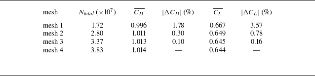
 b/h=5
 Reh=1000
 CD¯
 CL¯
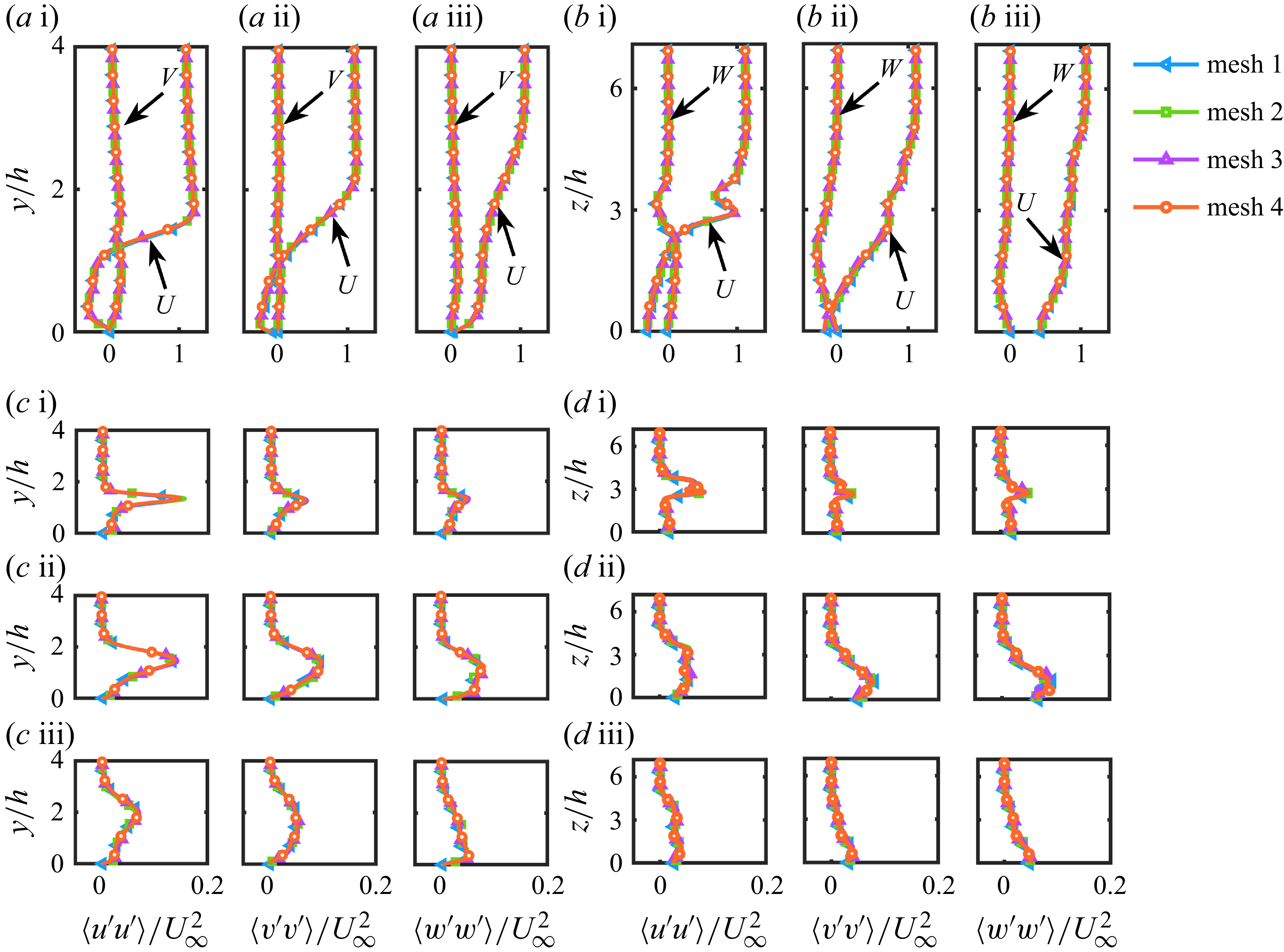
 b/h=5
 Reh=1000
 (a,c)
 z/h=0
 (b,d)
 y/h=0.5
 (a)
 U
 V
 (b)
 U
 W
 (c,d)
 x/h=1
 x/h=3
 x/h=7
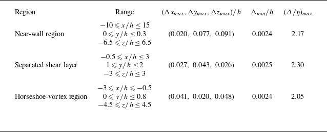
 b/h=5
 Reh=1000
 h

 Δ/η
 b/h=5
 Reh=1000
 (a)
 z/h=0
 (b)
 y/h=0.5

 AR=4
 h/b=4
 Reb=1000
 (a
 c)
 x/b=3
 (a)y/b=1
 (b)y/b=2
 (c)y/b=3
 (d
 f)
 x/b=7
 y/b=3
 (d)
 (e)
 (f)

 (a
 c)
 Reh=300
 Q=0.1
 u/U∞
 (a)
 Q=0.025
 (d
 f)
 (a−c)
 z/h=0
 x/h<−0.5
 ωz
 x/h>−0.5
 ωx
 (a,d)b/h=1
 (b,e)b/h=3
 (c,f)b/h=5

 y/h=0.3
 Reh=300
 (a)b/h=1
 (b)b/h=3
 (c)b/h=5

 (a
 c)
 Reh=500
 Q=0.1
 u/U∞
 (d
 f)
 b/h=1
 b/h=3
 b/h=5

 y/h=0.3
 Reh=500
 (a)b/h=1
 (b)b/h=3
 (c)b/h=5

 (a
 c)
 Reh=1000
 Q=0.1
 u/U∞
 (d
 f)
 b/h=1
 b/h=3
 b/h=5

 Reh=1000

 (a)
 A/h2
 b/h=1
 b/h=3
 b/h=5
 (b,c)
 z/h=0.3
 b/h=1
 b/h=5
 Reh=300
 Reh=500
 Reh=1000
 (b)
 (c)

 (a)
 Reh=500
 z/h
 x
 z
 b/h=1
 b/h=3
 b/h=5
 z
 y
 ωx
 (b)
 x/h=0.5
 ωx
 Reh=500
 b/h=1
 b/h=3
 b/h=5
 (c)
 (a)

 Reh=300
 b/h=3
 (a)
 M1(2,1.5,0)
 M2(4.5,1.8,0)
 M3(8.5,2.15,0)
 M4(10.5,2.8,0)
 M5(14,1.2,0.6)
 St0=0.146
 (b)
 St0
 ±0.0006
 (c)
 M5
 (d)
 Q
 Q=0.1
 ωx
 z
 y
 ωx
 t=t0
 t=t0+Δt
 t=t0+2Δt
 Δt=1.75
 (e)
 (c)
 t=t1
 t=t2
 t=t3
 M5

 Reh=300
 b/h=5
 M1(2,1.6,0)
 M2(7,1.8,1.65)
 M3(8.8,1.8,0)
 M4(11,2.6,0)
 M5(14,2.6,0)
 St0=0.202
 M3
 ϕ1
 ϕ2
 (b)
 ±0.0006
 St0
 St0/2
 (c)
 M2
 ϕ1
 ϕ2
 Q
 Q=0.1
 M2
 (d)
 St0
 St0/2
 Q
 Q=0.1

 Reh=500
 b/h=1
 M1(1,1.6,0)
 M2(3.45,1.5,0)
 M3(3.4,0.8,1)
 M4(6,1.7,0)
 M5(10,2,0)
 St0=0.211
 (b)
 St0
 ±0.0006
 Q
 Q=0.1
 ωx

 Reh=500
 b/h=3
 5
 (a)
 b/h=3
 M1(1.5,1.7,0)
 M2(4,1.7,0)
 M3(6,1.9,0)
 M4(8,1.9,0)
 M5(10,1.9,0)
 St01=0.267
 St02=0.287
 (b)
 b/h=5
 M1(1.5,1.8,0)
 M2(4,1.8,0)
 M3(6.5,2,0)
 M4(8.5,2.2,0)
 M5(10,0.6,2.4)
 St01=0.244
 St02=0.280
 (c,d)
 ±0.0006
 St01
 St02
 Q=0.1
 (c)b/h=3
 (d)b/h=5

 Reh=1000
 b/h=1
 (a)
 M1(0.9,1.6,0)
 M2(0.5,0.55,1)
 M3(2,0.6,1.3)
 M4(3.1,0.45,1.75)
 M5(6,1.5,0)
 M6(10,1.5,0)
 St01=0.620
 St02=0.696
 (b)
 ±0.0006
 St01
 St02
 (c)
 Q
 Q=0.1
 ωx
 (di)
 St01/4
 ±0.0006
 Q
 Q=0.1
 t=t0
 t=t0+Δt
 t=t0+2Δt
 Δt=3.2
 M5
 M6

 Reh=1000
 b/h=3
 (a)
 M1(−1.35,0.25,0)
 M2(−0.9,0.6,0)
 M3(−0.2,1.1,0)
 M4(0.55,1.9,0)
 M5(4,2,0)
 M6(8,2,0)
 St1=0.108
 St2=0.128
 (b)
 ±0.0006
 St1
 St2
 (c)
 Q
 Q=0.1
 ωz
 t=t0
 t=t0+Δt
 t=t0+2Δt
 t=t0+3Δt
 t=t0+4Δt
 t=t0+5Δt
 Δt=3
 ωz
 ωz

 Reh=1000
 b/h=5
 (a)
 M1(−1.7,0.4,0)
 M2(−0.9,0.7,0)
 M3(0,1.4,0)
 M4(3.5,2.3,0)
 M5(7.5,3,0)
 (b)
 ±0.0006
 St1
 St2
 St3
 St4
 (a)
 (c)
 Q
 Q=0.1
 ωz
 ωz
 ωz

 (Reh,b/h)


 Reh=1000
 (a)
 (b)
 ⟨u′u′⟩
 (c)
 ⟨v′v′⟩
 (d)
 ⟨w′w′⟩
 b/h=1
 b/h=3
 b/h=5
 0.04

 b/h=1
 b/h=3
 b/h=5

 z
 y
 Reh=1000
 (a)
 (b)
 ⟨u′u′⟩
 (c)
 ⟨v′v′⟩
 (d)
 ⟨w′w′⟩
 b/h=1
 b/h=3
 b/h=5

 −⟨u′v′⟩
 Reh=1000
 (a)
 (b)
 z
 y
 (c)
 −⟨u′v′⟩
 b/h=1
 b/h=3
 b/h=5

 Reh=1000
 (a)
 P11+P22+P33
 (b)
 P11
 b/h=1
 b/h=3
 b/h=5

 z
 y
 Reh=1000
 (a)
 P11+P22+P33
 (b)
 P11
 b/h=1
 b/h=3
 b/h=5

 z
 y
 Reh=1000
 (a)
 Π11
 (b)
 Π22
 (c)
 Π33
 b/h=1
 b/h=3
 b/h=5

 Reh=300
 (a)b/h=3
 (b)b/h=5
 0.04

 Reh=500
 (a)
 z/h=0
 (b)z
 y
 b/h=1
 3
 5
 0.04


