


1. Introduction
How effective are individual transferable quotas (ITQs)Footnote 1 in promoting sustainable resource use when agents face credit constraints and act as both producers and consumers? While ITQs are well studied – especially in fisheries – most general equilibrium models abstract from the institutional frictions and household-level complexities typical of developing economies. In particular, Jouvet and Rotillon (Reference Jouvet and Rotillon2005) consider representative agents with full market access, which limits the relevance of their framework for settings where agricultural households dominate and credit markets are incomplete.
This article fills that gap by embedding the agricultural household model into an overlapping generations (OLG) framework with renewable resources in order to test whether ITQs achieve intergenerational efficiency under credit constraints and household heterogeneity. It makes three contributions. First, it extends Jouvet and Rotillon (Reference Jouvet and Rotillon2005) by distinguishing wage earners from agricultural households subject to market imperfections. Second, it shows that ITQs alone cannot ensure efficient long-run resource use when credit markets are imperfect. Third, it highlights the need for complementary policies, especially improved financial access, to strengthen ITQ effectiveness in developing economies.
The overuse of renewable resources – fisheries (Worm et al., Reference Worm, Barbier, Beaumont, Duffy, Folke, Halpern, Jackson, Lotze, Micheli and Palumbi2006; Sumaila et al., Reference Sumaila, Cheung, Lam, Pauly and Herrick2011), forests (Crespo Cuaresma et al., Reference Crespo Cuaresma, Danylo, Fritz, McCallum, Obersteiner, See and Walsh2017) and freshwater systems (WWAP/UN-Water, 2018; Mohamed and Al-Mulali, Reference Mohamed and Al-Mulali2020) – threatens sustainable development. As a market-based instrument, ITQs align conservation with efficiency (Anderson, Reference Anderson2008) and often outperform Pigouvian taxes and input rationing, especially under stock uncertainty, selection and intergenerational concerns (Mahé and Ropars, Reference Mahé and Ropars2001; Jouvet and Rotillon, Reference Jouvet and Rotillon2005; Dresdner et al., Reference Dresdner, Campos and Chavez2010). Yet their effectiveness in developing economies remains unclear (Hoshino et al., Reference Hoshino, van Putten, Pascoe and Vieira2020).
Understanding resource management in developing economies requires analyzing agricultural households, which dominate rural employment and operate under pervasive market imperfections, especially credit constraints (De Janvry and Sadoulet, Reference De Janvry, Sadoulet, de Janvry and Kanbur2006; Ali et al., Reference Ali, Deininger and Duponchel2014; Chen et al., Reference Chen, Zeng, Zhang and Kang2020; Peng Yl et al., Reference Peng, Yanjun and Hj2021; Peng et al., Reference Peng, Wang and Zhou2022). The agricultural household model captures their joint production and consumption decisions and the role of frictions and risk in shaping resource allocation across production, consumption and investment (Singh et al., Reference Singh, Squire and Strauss1986a; Benjamin, Reference Benjamin1992; Sadoulet, Reference Sadoulet2000; Ditzler et al., Reference Ditzler, Komarek, Chiang, Alvarez, Chatterjee, Timler, Raneri, Carmona, Kennedy and Groot2019). A growing literature uses this framework to study how credit constraints affect productivity, technology adoption, income diversification and welfare (Malchow-Moeller and Thorsen, Reference Malchow-Moeller and Thorsen2000; Zhao et al., Reference Zhao, Zhang and Barry2014; Moahid and Maharjan, Reference Moahid and Maharjan2020).
Among the many market imperfections facing agricultural households – insecure land rights, information asymmetries and technological barriers – this study focuses on credit constraints because they are pervasive, analytically tractable and policy relevant, and are well documented in rural economies where they affect investment, technology adoption and resilience, e.g., (Ali et al., Reference Ali, Deininger and Duponchel2014; Chen et al., Reference Chen, Zeng, Zhang and Kang2020; Peng et al., Reference Peng, Wang and Zhou2022). Focusing on credit clarifies the mechanisms at play and directly informs complementary policies, such as financial inclusion, that can strengthen ITQs and improve resource management.
The analysis assesses ITQs as an instrument for intertemporal resource regulation – one that aims to preserve stocks, maximize the current generation’s welfare and ensure intergenerational equity – within a sustainable developmentFootnote 2 perspective that integrates the environmental, economic and social dimensions of well-being (Jouvenel Bd, Reference Jouvenel1970; Passet, Reference Passet1979).
This paper adds to the literature on ITQs and the restoration of the social optimum in renewable-resource use (Grafton et al., Reference Grafton, Squires and Fox2000; Mahé and Ropars, Reference Mahé and Ropars2001; Pinkerton and Edwards, Reference Pinkerton and Edwards2009), employing a general equilibrium framework with intergenerational transfers (Jouvet and Rotillon, Reference Jouvet and Rotillon2005). ITQs outperform input rationing (Mahé and Ropars, Reference Mahé and Ropars2001), yet remain insufficient for full sustainability without well-defined property rights (Arnason, Reference Arnason2012); weak regulation risks market power concentration (Anderson, Reference Anderson2008), and persistent equity and distributional challenges also limit their effectiveness (Hoshino et al., Reference Hoshino, van Putten, Pascoe and Vieira2020).
Our approach extends Jouvet and Rotillon (Reference Jouvet and Rotillon2005) by introducing agricultural households – agents who are both producers and consumers (Singh et al., Reference Singh, Squire and Strauss1986a; Benjamin, Reference Benjamin1992; Ditzler et al., Reference Ditzler, Komarek, Chiang, Alvarez, Chatterjee, Timler, Raneri, Carmona, Kennedy and Groot2019) – and incorporating credit constraints. Agricultural household models capture how price changes can generate counterintuitive responses through the profit effect (Chayanov, Reference Chayanov and Irwin1925; Singh et al., Reference Singh, Squire and Strauss1986b), a feature that standard neoclassical models cannot accommodate (Deaton, Reference Deaton1989).
Within this framework, we compare the competitive equilibrium with the social optimum. The results show that transferable quotas alone are insufficient to secure environmental preservation when credit constraints bind, since they prevent the economy from reaching the efficient allocation without welfare costs. Effective policy must therefore include improved access to finance.
The rest of this paper is structured as follows. Section 2 constructs a theoretical framework involving overlapping generations of credit-constrained agricultural households. Section 3 offers an analytical resolution of the model. Section 4 examines the model’s equilibrium. Section 5 concludes and discusses directions for future research.
2. Model architecture
We adopt an OLG model with a renewable natural resource and no demographic growth, similar to Jouvet and Rotillon (Reference Jouvet and Rotillon2005). In each period, a constant population of  $N$ identical individuals is born, forming a cohort. Individuals live for two periods:
 $t$ and
 $t+1$. In the first period, they work, consume and save. In the second period, they are retired and finance consumption through savings accumulated during youth. This perpetual process ensures overlapping generations at any point in time. Time is discrete and infinite.
Individuals born in period  $t$ are simultaneously producers and consumers. Their economic role requires integrated decisions regarding production inputs, consumption and intertemporal investment, taking into account market constraints and risk factors that affect these choices.
In line with Jouvet and Rotillon (Reference Jouvet and Rotillon2005), production relies on a renewable natural resource managed by the government. The government periodically issues a fixed quantity  $\bar{E}$ of transferable exploitation quotas, initially distributed to the young generation. Unlike Jouvet and Rotillon (Reference Jouvet and Rotillon2005), however, we focus on a setting in which agriculture is carried out by agricultural households.
A practical interpretation of this framework is the allocation of water quotas for irrigation in agriculture, a resource that is notably scarce in many developing countries. In this setting, households receive transferable quotas that can be used in production or traded in secondary markets. This mechanism encourages more judicious resource use and provides a concrete way to study the interaction between environmental regulation and household finance.
Several real-world institutional settings help illustrate the mechanisms formalized in this model. Chile’s tradable water-rights system is a relevant institutional analogue, as water allocations are transferable and may be exchanged in secondary markets, although participation and trading conditions may vary across users (Bauer, Reference Bauer2004; Donoso, Reference Donoso2006). In fisheries, South Africa’s ITQ system has been associated with distributional concerns and limited access for small-scale fishers (Isaacs, Reference Isaacs2011), a pattern that is broadly consistent with the leasing-versus-selling margin emphasized in the model. Taken together, these examples suggest that the performance of transferable quota systems may depend on the institutional environment in which they operate, including the extent of access to finance, which the analysis below examines formally.
This study focuses on agricultural households that engage in both production and consumption, as outlined in the seminal works of Singh et al. (Reference Singh, Squire and Strauss1986a) and Benjamin (Reference Benjamin1992). The agricultural household model consists of two modules, namely the production module and the consumption module, which are linked by the individual’s time use constraint. The production module describes how individuals allocate resources and technology to produce agricultural goods, while the consumption module describes how they derive utility from these goods and other market commodities.
2.1. Preferences and technology
All households share identical preferences represented by a twice-differentiable, concave and time-separable intertemporal utility function:
 \begin{equation}
V = U(c_t, \ell_t ; X_t) + \beta U(d_{t+1}, X_{t+1}).
\end{equation}
The functions  $U(\cdot)$ are instantaneous utility functions, continuous and strictly concave, for which, for any argument
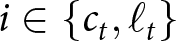 $i \in \{c_t,\ell_t\}$,
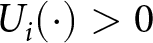 $U_i(\cdot) \gt 0$ and
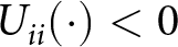 $U_{ii}(\cdot) \lt 0$.
 $c_t$ and
 $\ell_t$ denote consumption and leisure of the individual in the first period of life, when young. The biomass stock present in period
 $t$,
 $X_t$, is a state variable inherited from the previous period. Similarly,
 $X_{t+1}$ represents the biomass stock in the subsequent period
 $t+1$. The utility function’s dependence on
 $X_{t+1}$ reflects the resource’s intrinsic value (Jouvet and Rotillon, Reference Jouvet and Rotillon2005). The variable
 $d_{t+1}$ denotes consumption for the same individual in the second life period, retirement. The parameter
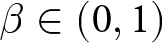 $\beta\in(0,1)$ represents the subjective discount factor of the economic agent, allowing future utility to be expressed in present-value terms. The higher
 $\beta$ is, the more important the future is.
The economy’s production is carried out by agricultural households in a perfectly competitive environment, using capital  $K$, labour
 $L$ and resource quotas
 $E$ to produce a consumption good
 $Y$. The aggregate production function is twice differentiable and exhibits constant returns to scale, and is written as:
 $Y_t = F( K_t, E_t, L_t)$. The hypothesis of constant returns to scale allows the production function to be written in intensive form as:
 \begin{equation}
y_t = f(k_t, e_t).
\end{equation}
This is the output per worker, with 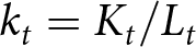 $k_t=K_t/L_t$,
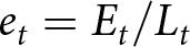 $e_t=E_t/L_t$ and
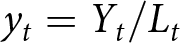 $y_t=Y_t/L_t$. The function
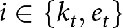
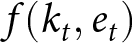 $f(k_t, e_t)$ satisfies the traditional properties (Lau, Reference Lau1976), such as for any argument
 $i \in \{k_t, e_t\}$,
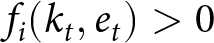 $f_i(k_t, e_t) \gt 0$ and
 $f_{ii}(k_t, e_t) \lt 0$, and for any
 $i \neq j$,
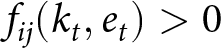 $f_{ij}(k_t, e_t) \gt 0$. Physical capital and the resource input are assumed to depreciate completely in the production process, so
 $\delta=1$.Footnote 3
Unlike Jouvet and Rotillon (Reference Jouvet and Rotillon2005), where each individual supplies one unit of labour inelastically in the first period, this paper adopts the agricultural household assumption of Singh et al. (Reference Singh, Squire and Strauss1986a) and Benjamin (Reference Benjamin1992). Each individual has a fixed time endowment  $T$, allocated between own-farm labour
 $n_t^i$ (in-farm labour), off-farm labour
 $n_t^o$ and leisure
 $\ell_t$, such that:
 \begin{equation}
T = n_t^i + n_t^o + \ell_t.
\end{equation}
This captures the trade-offs individuals face between competing activities. Total farm labour  $n_t$ is the sum of own-farm labour
 $n_t^i$ and hired labour
 $n_t^h$ supplied by wage earners:
 \begin{equation}
n_t= n_t^i + n_t^h.
\end{equation}
This assumption captures the flexibility provided by the labour market. Consequently, the individual can use the market to complement or substitute for their own labour, depending on the wage rate, the opportunity cost of time and marginal productivity. This framework allows agricultural households to adjust labour allocation in response to wages, time costs and marginal productivity.
It is assumed that the total population of the young generation in a period can be aggregated as: 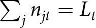 $\sum_j n_{jt} = L_t$, where
 $j$ indexes individuals.
2.2. The renewable natural resource
At each period, the renewable natural resource evolves according to the difference between net recruitment (natural renewal) and previous use:
 \begin{equation}
X_{t+1}=X_t + G(X_t) - E_t.
\end{equation}
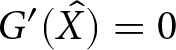
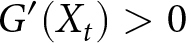
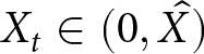
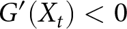
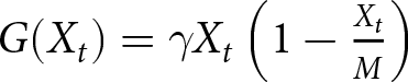
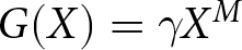
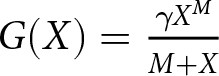
The net recruitment function  $G(X_t)$Footnote 4 satisfies the standard assumptions:
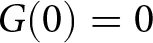 $G(0)=0$, there exists
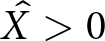 $\hat{X} \gt 0$ and
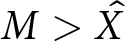 $M \gt \hat{X}$ such that
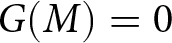 $G(M)=0$ and
 $G'(\hat{X})=0$, and
 $G'(X_t) \gt 0$ for
 $X_t\in(0,\hat{X})$ while
 $G'(X_t) \lt 0$ for
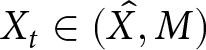 $X_t\in(\hat{X},M)$. Thus,
 $G(\hat{X})$ is the maximum sustainable yield, and
 $M$ is the virgin biomass level when the resource is unexploited. Without human intervention, if
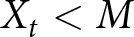 $X_t \lt M$, the stock will grow until it reaches
 $M$, where the net recruitment
 $G(X_t)$ is zero, signifying the natural equilibrium of the population.
2.3. Consumption of the cohort born in t when young
When young, an individual’s income comes from off-farm labour ( $w_t n_t^o$) and farm production (
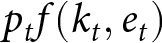 $p_t f(k_t, e_t)$). From this gross income, the individual deducts factor costs:
 $w_t n_t^h = w_t (n_t - n_t^i)$ for hired labour (with
 $w_t$ the wage,
 $n_t$ total farm labour and
 $n_t^i$ own labour),
 $r_t k_t$ for capital (with
 $r_t$ the return on capital) and
 $\phi_t e_t$ for the natural resource (with
 $\phi_t$ its rental rate). The remaining income is allocated to consumption
 $c_t$, physical capital savings
 $s_t$ and exploitation quotas
 $e_t$, purchased on the secondary market at price
 $q_t$. Normalizing the output price to one, the first-period cash-flow constraint is:
 \begin{equation}
c_t + s_t + q_t e_t = f(k_t, e_t) - R_t k_t - \phi_t e_t - w_t n^h_t + w_t n_t^o
\end{equation}
with  $R_t = 1 + r_t$, given the complete depreciation of capital in the production process. Substituting constraints
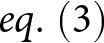 $eq.~(3)$ and
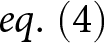 $eq.~(4)$ into
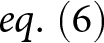 $eq.~(6)$ yields the global income constraint:
 \begin{equation}
c_t + s_t + q_t e_t + w_t \ell_t = f(k_t, e_t) - R_t k_t - \phi_t e_t - w_t n_t + w_t T.
\end{equation}
This equation states that young-age income is allocated to consumption, savings, quota purchases and leisure. Total income includes non-maximized agricultural profits ( $\psi_t = f(\cdot) - R_t k_t - \phi_t e_t - w_t n_t$), and the opportunity cost of time endowment.
The individual’s savings decision ( $s_t$) provides the source of capital for production in the subsequent period,
 $t+1$. The aggregate capital stock
 $K_{t+1}$ available to the next generation of producers is generally determined by the current young generation’s total savings
 $N s_t$ and the undepreciated capital stock from the previous period,
 $K_t$ (i.e., the law of motion for capital):
 $K_{t+1} = N s_t + (1-\delta)K_t$. Given the assumption of complete depreciation of capital in the production process (
 $\delta=1$), the capital accumulation equation simplifies to
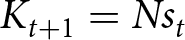 $K_{t+1} = N s_t$ or, in terms per-worker (assuming a constant population
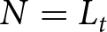 $N=L_t$),
 \begin{equation}
k_{t+1} = s_t.
\end{equation}
This equation establishes the dynamic link between the individual’s current savings decision and the capital stock available to the economy in the following period.
2.4. Credit constraint
Agricultural producers in developing economies frequently face credit constraints when financing production inputs (Guirkinger and Boucher, Reference Guirkinger and Boucher2008; Ali et al., Reference Ali, Deininger and Duponchel2014). This section models how credit market imperfections affect the acquisition of the resource input  $\phi_t e_t$.
The credit constraint applies to the quota rental cost ( $\phi_t e_t$) for three main reasons: analytical tractability, realistic liquidity needs and policy relevance. Analytically, constraining only the regulated input captures how credit friction disrupts the separability between production and consumption. Realistically, resource access often requires a significant upfront payment – a liquidity requirement that is not covered by current income – distinguishing it from inputs like capital (
 $k_t$), which is financed internally via OLG savings (
 $s_t$). Finally, this formulation isolates the core interaction needed to assess whether financial inclusion must complement the ITQ system.
This credit structure adapts the collateral-based constraint literature (Guirkinger and Boucher, Reference Guirkinger and Boucher2008). The individual finances the resource input,  $\phi_t e_t$, by taking out a loan
 $B$, and lenders determine the maximum borrowing capacity from the value of titled land. Following Guirkinger and Boucher (Reference Guirkinger and Boucher2008), we assume a zero interest rate on loans, focusing on collateral constraints rather than interest-rate effects. The expenditures on the natural resource input are limited to the borrowing capacity:
 \begin{equation}
\phi_t e_t \leq B.
\end{equation}
Let  $\tau$ be the land price,
 $v$ the proportion of titled agricultural land, and
 $A_f$ the total landholding. The credit limit
 $B$ of an individual is constrained by the value of titled land:
 \begin{equation}
0 \leq B \leq \tau v A_f.
\end{equation}
2.5. Consumption of the cohort born in t when retired
Each period, the government allocates a quantity of natural resources equivalent to  $\bar{E}_t$ to the retiree generation. This quantity is distributed equally among all individuals, giving
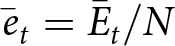 $\bar{e}_t=\bar{E}_t / N$ per individual. Thus, when retired, an individual born in period
 $t$ holds the sum of the government endowment and the quotas purchased on the secondary market:
 \begin{equation}
\tilde{e}_t = e_t + \bar{e}_t.
\end{equation}
This principle allows delayed resource exploitation. Only young individuals can buy permits, but they can sell them only at retirement. Upon retirement, individuals manage their quota holdings. They may sell a fraction 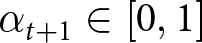 $\alpha_{t+1}\in[0,1]$ to the young generation at price
 $q_{t+1}$, or lease the remaining fraction to active producers at rental rate
 $\phi_{t+1}$. Rental income represents the return on the asset when it is used in production. Due to complete depreciation (
 $\delta=1$), quotas leased for production are extinguished after use. Consequently, the retired consumption (
 $d_{t+1}$) of an agent born in period
 $t$ is:
 \begin{equation}
d_{t+1} = R_{t+1} s_t + [\alpha_{t+1} \phi_{t+1} + (1-\alpha_{t+1}) q_{t+1}]\tilde{e}_t
\end{equation}
with  $R_{t+1}$ the capitalization factor of the invested savings,
 $\alpha_{t+1}$ the allocation parameter between quotas selling and leasing, and
 $[\alpha_{t+1} \phi_{t+1} + (1-\alpha_{t+1}) q_{t+1}]\tilde{e}_t$ the weighted average return on the quota asset. We assume that individuals have neither altruistic motives nor bequest motives. They therefore consume only for themselves at the end of life.
Individuals recognize the externalities that resource utilization in the production process imposes on stock dynamics. Overexploitation can lead to significant environmental degradation – including pollution, biodiversity loss and climate change – which can affect human health, quality of life and local economies. In a non-cooperative setting, each individual takes the actions of others as given. Let  $\bar{\varphi}_{t+1}$ denote aggregate use by all other individuals. The stock dynamics then become:
 \begin{equation}
X_{t+1}=X_t + G(X_t) - \alpha_{t+1} \tilde{e}_t - \bar{\varphi}_{t+1}.
\end{equation}
2.6. Overlapping generations model of agricultural household
Under the conditions described and the assumptions of the model, the problem of the individual consists in maximizing their utility (1) subject to the constraints of the global income of the first period (7), the global income of the second period (12), the dynamics of stock of the natural resource (13) and credit (9), with the condition on the credit limits (10):
 \begin{align*}
\underset{c_t, \ell_t, s_t, d_{t+1}, X_{t+1}, \alpha_{t+1}, k_t, n_t, e_t} {\max} \quad V & = U(c_t, \ell_t; X_t) + \beta U(d_{t+1}, X_{t+1}) \\
\text{s.t} \quad c_t + s_t + q_t e_t + w_t \ell_t & = f(k_t, e_t) - R_t k_t - \phi_t e_t - w_t n_t + w_t T \\
d_{t+1} & = R_{t+1} s_t + [\alpha_{t+1} \phi_{t+1} + (1-\alpha_{t+1}) q_{t+1}]\tilde{e}_t \\
X_{t+1} & = X_t + G(X_t) - \alpha_{t+1} \tilde{e}_t - \bar{\varphi}_{t+1}\\
\phi_t e_t & \leq B\\
\text{with} \quad 0\leq B \leq \tau v A_f \quad & \text{and} \quad c_t, \ell_t, s_t, d_{t+1}, X_{t+1}, \alpha_{t+1}, k_t, n_t, e_t \geq 0.
\end{align*}
3. Programme resolution
The Lagrangian of this agricultural agent’s programme is written as:
 \begin{align*}
\mathcal{L} = & U(f(k_t, e_t) - R_t k_t - \phi_t e_t - w_t n_t + w_t T - s_t - q_t e_t - w_t \ell_t ,\ \ell_t; X_t) \\
& + \beta U(R_{t+1} s_t + [\alpha_{t+1} \phi_{t+1} + (1-\alpha_{t+1}) q_{t+1}]\tilde{e}_t,\ X_t + G(X_t) - \alpha_{t+1} \tilde{e}_t - \bar{\varphi}_{t+1}) \\
& + \lambda_t \left(B -\phi_t e_t \right)
\end{align*}
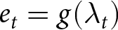
with 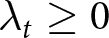 $\lambda_t \geq 0$ the Lagrange multiplier, which is the fictitious price of the credit constraint. The first-order conditions (FOCs) with respect to
 $\ell_t,\ s_t$ and
 $\alpha_{t+1}$ – the variables of the consumption module – characterize the main trade-offs faced by the individual. These conditions correspond to:
(1) The trade-off between consumption and leisure when the individual is young:
(14) \begin{equation}
U_{\ell_t}(c_t, \ell_t; X_t) = w_t U_{c_t}(c_t, \ell_t; X_t).
\end{equation}
This standard tangency condition states that, at the optimum, the marginal rate of substitution between consumption and leisure equals the real wage.
(2) The trade-off between consumption over the life cycle:
(15)\begin{equation}
U_{c_t}(c_t, \ell_t; X_t) = \beta R_{t+1} U_{d_{t+1}}(d_{t+1}, X_{t+1}).
\end{equation}This is the standard Euler equation. It equates the marginal utility cost of saving today with the discounted marginal utility benefit of consuming tomorrow.
(3) The trade-off, when the individual is retired, between selling the quotas to the future generation and using them in the production process:
\begin{equation*}
(\phi_{t+1} - q_{t+1}) \tilde{e}_t \beta U_{d_{t+1}}(d_{t+1}, X_{t+1}) - \tilde{e}_t \beta U_{X_{t+1}}(d_{t+1}, X_{t+1})=0.
\end{equation*}Rearranging this expression yields the quota price:
(16)\begin{equation}
q_{t+1} = \phi_{t+1} - \frac{U_{X_{t+1}}(d_{t+1}, X_{t+1})}{U_{d_{t+1}}(d_{t+1}, X_{t+1})}.
\end{equation}The price differential
$(\phi_{t+1} - q_{t+1})$ reflects the trade-off retirees face between leasing quotas to active producers at rental rate
$\phi_{t+1}$ versus selling them permanently to the young generation at asset price
$q_{t+1}$ for savings. Retirees optimize this allocation while internalizing the environmental externality through the term
$U_{X_{t+1}}(\cdot)/U_{d_{t+1}}(\cdot)$. A positive differential (
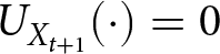
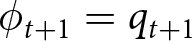
$\phi_{t+1} - q_{t+1} \gt 0$) incentivizes leasing over selling, which maximizes individual returns but exacerbates environmental degradation (Farrell, Reference Farrell2008). By recognizing this negative externality on resource stocks, retirees internalize the environmental cost through the price gap. However, if retirees are indifferent to environmental quality (
$U_{X_{t+1}}(\cdot) = 0$), this internalization disappears and
$\phi_{t+1} = q_{t+1}$.


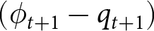




In the production module, the FOCs with respect to  $k_t$,
 $n_t$ and
 $e_t$ are given by:
(1) The marginal product of capital is given by:
(17)implying that the marginal product of capital\begin{equation}
R_t = F_{K_t}(K_t, E_t, L_t) = f_{k_t}(k_t, e_t)
\end{equation}
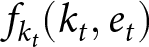
$f_{k_t}(k_t, e_t)$ equals the rental rate of capital
$R_t$, satisfying the standard profit-maximizing condition.(2) The marginal product of labour is found as follows:
(18)\begin{equation}
w_t = F_{L_t}(K_t, E_t, L_t)= f(k_t, e_t) - k_t f_{k_t}(k_t, e_t) - e_t f_{e_t}(k_t, e_t).
\end{equation}The wage
$w_t$ equals output per worker net of capital and resource payments.(3) The price of the resource is implicitly determined by the following expression:
which, after development, using Equations (15) and (16), as well as the property
\begin{align*}
U_{c_t}(\cdot)\left[f_{e_t}(\cdot) - \phi_t - q_t \right] &+ \beta U_{d_{t+1}}(\cdot) \left[ \alpha_{t+1}\phi_{t+1} + (1 - \alpha_{t+1}) q_{t+1} \right] \\
&- \beta \alpha_{t+1} U_{X_{t+1}}(\cdot)- \lambda_t \phi_t =0
\end{align*}
$R_{t+1} = q_{t+1}/q_t$, can be written as:
(19)\begin{equation}
\phi_t = f_{e_t}(\cdot)\left( \frac{U_{c_t}(\cdot)}{U_{c_t}(\cdot)+\lambda_t}\right).
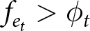
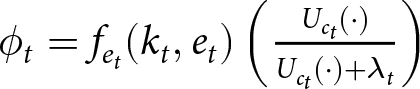
\end{equation}This equation characterizes the producer’s optimal choice under financial distress. When the credit constraint binds, the agent stops extracting at a point where the marginal product of the resource still exceeds its effective price (
$f_{e_t} \gt \phi_t$). The shadow price
$\lambda_t$ therefore represents a ‘liquidity wedge’: the marginal unit of the resource is profitable but financially unattainable.






The Karush–Kuhn–Tucker (KKT) conditions are:
 \begin{equation}
\lambda_t (B - \phi_t e_t) = 0
\end{equation}
 \begin{equation}
B - \phi_t e_t \geq 0
\end{equation}
 \begin{equation}
\lambda_t \geq 0.
\end{equation}
When the credit constraint is not binding (that is,  $B - \phi_t e_t \gt 0$ and therefore
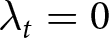 $\lambda_t=0$), condition (19) implies that the effective resource price equals its marginal product:
 \begin{equation}
\phi_t = f_{e_t}(k_t, e_t).
\end{equation}
In this context, the FOCs associated with the production factors indicate that, at the optimum, the individual chooses the optimal quantities of each factor, namely 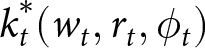 $k^*_t(w_t, r_t, \phi_t)$,
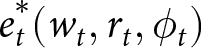 $e^*_t(w_t, r_t, \phi_t)$ and
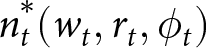 $n^*_t(w_t, r_t, \phi_t)$, so as to equate their marginal product in value to their market price. These results are consistent with the findings of Jouvet and Rotillon (Reference Jouvet and Rotillon2005). Therefore, the solution obtained is consistent with the standard ‘separability result’Footnote 5 (Singh et al., Reference Singh, Squire and Strauss1986a; De Janvry et al., Reference De Janvry, Fafchamps and Sadoulet1991; Benjamin, Reference Benjamin1992; Jacoby, Reference Jacoby1993; Udry, Reference Udry1996; Vakis et al., Reference Vakis, Sadoulet, De Janvry and Cafiero2004; LaFave and Thomas, Reference LaFave and Thomas2016) according to which: a) profit maximization is done independently of individual characteristics or preferences; b) business decisions enter the individual’s consumption-leisure decision only through the budget constraint; c) optimal quantities of production factors are determined only by their prices and production technology, and are not influenced by individual preferences; and d) profit maximization is separable from utility maximization.
In the presence of a binding credit constraint for the individual (i.e.,  $B - \phi_t e_t = 0$ and thus
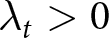 $\lambda_t \gt 0$), the optimality condition with respect to the price of the resource (19) shows that
 $\phi_t \lt f_{e_t}(d_{t+1}, X_{t+1})$, due to the strict positivity of
 $\lambda_t$ and
 $U_{c_t}(\cdot)$. More precisely:
 \begin{equation}
\phi_t = \frac{B}{e_t} = f_{e_t}(\cdot)\left( \frac{U_{c_t}(\cdot)}{U_{c_t}(\cdot)+\lambda_t}\right) \lt f_{e_t}(\cdot).
\end{equation}
Thus, the marginal product of the resource exceeds its market value, and production and consumption are no longer separable. As a result, production is subject to fluctuations in the fictitious price of the credit constraint and changes in individual preferences. Despite the individual’s intention to augment their production and profit by enhancing the quantity of factor  $e_t$, they are constrained by the saturated credit limit they encounter.
Differentiating Equation (24) with respect to the shadow price of credit,  $\lambda_t$, shows that the demand for the resource input falls as the constraint becomes tighter:Footnote 6
 \begin{equation*}
\left\{U_{c_t c_t}(\cdot) \left[ f_{e_t}(\cdot) -\phi_t \right]^2 + U_{c_t}(\cdot) f_{e_t e_t}(\cdot) \right\} \frac{d e_t}{d \lambda_t} = \phi_t.
\end{equation*}
Because 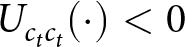 $U_{c_tc_t}(\cdot) \lt 0$ and
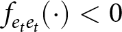 $f_{e_te_t}(\cdot) \lt 0$, it follows that:
 \begin{equation}
\frac{\mathrm{d} e_t}{\mathrm{d} \lambda_t} \lt 0.
\end{equation}
This captures the intuitive mechanism that constrained access to credit forces agricultural producers to reduce their utilization of financed inputs, thereby adjusting their production and consumption decisions in response to financial limitations. In contrast to unconstrained individuals, as referenced in Jouvet and Rotillon (Reference Jouvet and Rotillon2005), credit-constrained individuals are likely to underinvest in productivity-enhancing inputs, with implications for their incomes and livelihoods (Mukasa et al., Reference Mukasa, Simpasa and Salami2017).
4. Equilibrium analysis
This section characterizes the equilibrium behaviour of the OLG economy with agricultural households and a renewable natural resource regulated by ITQs. We first define the competitive equilibrium and derive the associated market-clearing conditions. We then characterize the steady-state equilibrium and its key properties. Building on this structure, we analyse how binding credit constraints distort prices, allocations and resource dynamics. Finally, we examine how financial policies that relax credit constraints affect equilibrium outcomes and compare the decentralized equilibrium with the social optimum.
4.1. Competitive equilibrium
4.1.1. Definition of equilibrium
A competitive equilibrium for this OLG economy of individuals operating as agricultural households with a renewable natural resource regulated by ITQs is a sequence of capital and natural resource stocks for production, consumption of goods in both periods, and leisure, physical capital and quota savings, biomass stock and resource sharing coefficient between production and resale  $\{k_t,$
 $\tilde{E}_{t+1},$
 $c_t,$
 $d_{t+1},$
 $\ell_t,$
 $s_t,$
 $e_t,$
 $X_{t+1},$
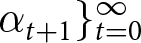 $\alpha_{t+1}\}_{t=0}^\infty$ and the set of prices (quota price, capital return, resource price, wage and credit constraint shadow price)
 $\{q_t,$
 $R_t,$
 $\phi_t,$
 $w_t,$
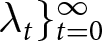 $\lambda_t\}_{t=0}^\infty$ such that, given prices, preferences and technology: a) quantities maximize agents’ utility subject to budget constraints of both periods, biomass dynamics constraint and credit constraint; and b) markets are in equilibrium.
The economy under examination includes five markets, namely the labour market, the natural resource market, the capital market, the goods market and the credit market. The equilibrium of the labour market implies the equality between the number of workers demanded in farms (demand) and the size of the young generation in the period (supply):
 \begin{equation}
\sum n_t = L_t = N.
\end{equation}
Retirees supply the natural resource input to the economy. They lease a quantity  $\tilde{E}_{t+1} = N\alpha_{t+1}(e_t + \bar{e}_t)$ to the active generation for immediate production. The remaining stock
 $Ne_{t+1} = N(1-\alpha_{t+1})(e_t + \bar{e}_t)$ is sold to the young generation to be held as savings for the next period. Thus, the total quantity of natural resource quotas actually used in production during period
 $t+1$ is determined by the difference between the total quantity of quotas held by retirees and the quantity of quotas sold to the younger generation,
 \begin{equation}
\tilde{E}_{t+1} = N(e_t - e_{t+1} + \bar{e}_t).
\end{equation}
Considering the above, the aggregate production function can be rewritten as  $Y_t = F(K_t, N(e_t - e_{t+1} + \bar{e}_t), N)$ or, in intensive form, as:
 \begin{equation}
y_t = f(k_t, (e_t - e_{t+1} + \bar{e}_t)).
\end{equation}
Therefore, the dynamics of the resource stock in (13) become:
 \begin{equation}
X_{t+1}=X_t + G(X_t) - N(e_t - e_{t+1} + \bar{e}_t).
\end{equation}
At the macroeconomic level, the goods market equilibrium implies equality between aggregate supply (economy’s production) and aggregate demand (aggregate consumption and investment demand). Formally,  $Nc_t + Nd_t + Ns_t = F(K_t, E_t, L_t)$, which is expressed in intensive form as:
 \begin{equation}
c_t + d_t + s_t = f(k_t, (e_t - e_{t+1} + \bar{e}_t)).
\end{equation}
The capital market clears when the aggregate demand for capital by active producers in period  $t+1$,
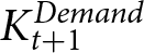 $K_{t+1}^{Demand}$, equals the aggregate supply of capital provided by the savings (
 $N s_t$) of the young cohort from period
 $t$,
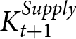 $K_{t+1}^{Supply}$. Given the assumption of complete depreciation of capital (
 $\delta=1$), the market clearing condition is equivalent to the capital accumulation Equation (8) established in Section 2.3.
Equilibrium in the credit market implies that:
 \begin{equation}
\phi_t e_t = B.
\end{equation}
Given all of the above, the equilibrium of this economy is defined by a system of 14 equations in 14 variables ( $k_t$,
 $\tilde{E}_{t+1}$,
 $c_t$,
 $\ell_t$,
 $d_{t+1}$,
 $s_t$,
 $e_t$,
 $X_{t+1}$,
 $\alpha_{t+1}$,
 $q_t$,
 $R_t$,
 $\phi_t$,
 $w_t$ and
 $\lambda_t$):
 \begin{equation}
\tilde{E}_{t+1} = N(e_t - e_{t+1} + \bar{e}_t)
\end{equation}
 \begin{equation}
k_{t+1} = s_t
\end{equation}
 \begin{equation}
R_t = \frac{q_t}{q_{t-1}}
\end{equation}
 \begin{equation}
R_t = f_{k_t} (k_t, (e_t - e_{t+1} + \bar{e}_t))
\end{equation}
 \begin{equation}
\phi_t = f_{e_t}(k_t, (e_t - e_{t+1} + \bar{e}_t)) \left[ \frac{U_{c_t}(c_t, \ell_t; X_t)}{U_{c_t}(c_t, \ell_t; X_t) + \lambda_t} \right]
\end{equation}
 \begin{equation}
w_t = f(\cdot) - k_t f_{k_t}(\cdot) - (e_t - e_{t+1} + \bar{e}_t) f_{e_t}(\cdot)
\end{equation}
 \begin{equation}
U_{\ell_t}(c_t, \ell_t; X_t) = w_t U_{c_t}(c_t, \ell_t; X_t)
\end{equation}
 \begin{equation}
U_{c_t}(c_t, \ell_t; X_t) = \beta R_{t+1} U_{d_{t+1}}(d_{t+1}, X_{t+1})
\end{equation}
 \begin{equation}
q_{t+1} = \phi_{t+1} - \frac{U_{X_{t+1}}(d_{t+1}, X_{t+1})}{U_{d_{t+1}}(d_{t+1}, X_{t+1})}
\end{equation}
 \begin{equation}
X_{t+1} =X_t + G(X_t) - N(e_t - e_{t+1} + \bar{e}_t)
\end{equation}
 \begin{equation}
c_t + d_t = f(k_t, (e_t - e_{t+1} + \bar{e}_t)) - k_{t-1}
\end{equation}
 \begin{equation}
c_t + s_t + q_t e_t + w_t \ell_t = w_t T
\end{equation}
 \begin{equation}
d_{t+1} = R_{t+1} s_t + [\alpha_{t+1} \phi_{t+1} + (1-\alpha_{t+1}) q_{t+1}] (e_t + \bar{e}_t)
\end{equation}
 \begin{equation}
\phi_t (e_t - e_{t+1} + \bar{e}_t) = B
\end{equation}
4.2. Steady state and dynamics of the model
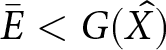
In each period, the government issues a fixed quantity of quotas, 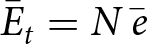 $\bar{E}_t = N\,\bar{e}$, distributed to the young generation at an allocation of
 $\bar{e}$ per individual. This policy is exogenous and designed to ensure the sustainability of the biomass by keeping quota issuance below the natural regeneration rate,
 $\bar{E} \lt G(\hat{X})$. At the steady state, (32) becomes:
 \begin{equation}
\tilde{E}^* = N\,\bar{e} = \bar{E},
\end{equation}
indicating that the entire quota endowment (received from the government) is used for production in the long-run equilibrium.
Equation (34) implies that the gross return on capital at the steady state is:
 \begin{equation}
R^* = 1.
\end{equation}
Equation (35) then simplifies to 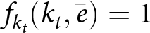 $f_{k_t}(k_t, \bar{e})=1$, which allows capital to be expressed as a function of the individual quota endowment
 $\bar{e}$:
 \begin{equation}
k^* = k\,(\bar{e})
\end{equation}
and therefore determine long-term savings using (33):
 \begin{equation}
s^* = k^*.
\end{equation}
It is possible to determine the long-term values for the resource price for production ( $\phi^*$) by using the equation for the production quotas (46) in (45) as
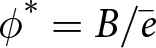 $\phi^* = B/\bar{e}$; this implies:
 \begin{equation}
B = \phi^*\,\bar{e}.
\end{equation}
The long-term wage ( $w^*$) is obtained by using the equations concerning the production quotas (46), the return of capital (47) and capital itself (48) in (37):
 \begin{equation}
w^* = f(k^*, \bar{e}) - k^* - \bar{e} f_{e}(k^*, \bar{e}).
\end{equation}
Knowing (46), it is possible, using Equation (41), to determine the long-term stock level  $X^*$ as a function of individual quota endowment
 $\bar{e}$ as follows:
 \begin{equation}
G(X^*) = N\bar{e}.
\end{equation}
Given 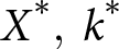 $X^*,\ k^*$ and
 $w^*$, steady-state consumption of goods (
 $c^*$ and
 $d^*$) and leisure (
 $\ell^*$) are determined by solving the system of Equations (38), (39) and (42) as follows:
 \begin{equation}
U_{\ell}(c^*, \ell^*; X^*) = w^* U_{c}(c^*, \ell^*; X^*)
\end{equation}
 \begin{equation}
U_{c}(c^*, \ell^*; X^*) = \beta U_d (d^*, X^*)
\end{equation}
 \begin{equation}
c^* + d^* = f(k^*, \bar{e}) - k^*.
\end{equation}
The expression for the long-term price of the quota in the secondary market is determined as follows, using  $d^*$,
 $X^*$ and
 $\phi^*$ in (40),
 \begin{equation}
q^* = \phi^* - \frac{U_X(d^*, X^*)}{U_d(d^*, X^*)}.
\end{equation}
The long-term quantity of quotas put on the resale market  $e^*$ is found as follows, using (43):
 \begin{equation}
e^* = \frac{1}{q^*} \left[w^*(T - \ell^*) - c^* - k^* \right].
\end{equation}
Consequently, in the steady state, the share of quotas allocated to the production process is implicitly determined by the consumption (44), which describes the consumption of an agent born in period  $t$ when retired:
 \begin{equation}
d^* =k^* + [\alpha (\phi^* - q^*) + q^*](e^* + \bar{e}).
\end{equation}
Finally, the shadow price of the long-term credit constraint,  $\lambda^*$, is derived from Equation (36) and is expressed as
 $\lambda^* = U_c(c^*, \ell^*; X^*) \left(\frac{f_e(k^*,\bar{e})}{\phi^*} - 1\right)$. This relationship can be reformulated to yield:
 \begin{equation}
\phi^* = f_e(k^*,\bar{e}) \left( \frac{U_c(c^*, \ell^*; X^*)}{U_c(c^*, \ell^*; X^*) + \lambda^* } \right).
\end{equation}
All variables have been determined at the long-term equilibrium as a function of individual quota endowment  $\bar{e}$. The existence of a steady state ensures that the economy can achieve the maximum possible utility. In this equilibrium, prices reflect supply and demand perfectly, allowing efficient resource allocation.
It is therefore possible to easily compare results between the separable regime (where the credit constraint is not saturated) and the non-separable regime (where the credit constraint is saturated). This comparison can be made using comparative statics, which allows for an analysis of changes in variables and evaluation of each regime’s ability to restore the social optimum.
4.3. Credit constraints and steady-state dynamics
To characterize the impact of financial frictions, we distinguish between the separable regime ( $S$), where credit constraints are not tight, and the non-separable regime (
 $NS$), where they bind. Variables corresponding to these regimes are denoted with the indices
 $S$ or
 $NS$.
Under binding credit constraints (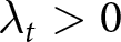 $\lambda_t \gt 0$), individuals demand less of the productive resource (according to Equation (25)), leading to a decrease in its price (
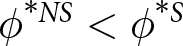 $\phi^{*NS} \lt \phi^{*S}$), as shown in Equation (59). Simultaneously, the increased supply of quotas in the secondary market lowers their price (
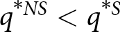 $q^{*NS} \lt q^{*S}$), according to Equation (56). While the absolute reductions in
 $\phi$ and
 $q$ are equal in magnitude, the relative declines differ because
 $q^*$ is initially smaller than
 $\phi^*$. A fixed absolute decrease in
 $q^*$ thus represents a proportionally larger decline compared to
 $\phi^*$, which can be expressed as
 $|\mathrm{d}q^* / q^*| \ \gt \ |\mathrm{d} \phi^* / \phi^*|$.
The decrease in  $q^*$ incentivizes the younger generation to save more in natural resources (
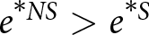 $e^{*NS} \gt e^{*S}$). This is evident from Equation (57), which indicates that a lower
 $q^*$ results in a higher
 $e^*$. However, this effect is counterbalanced for retirees, who are more inclined to lease their quotas to active producers, given that
 $|\mathrm{d}q^* / q^*| \ \gt \ |\mathrm{d} \phi^* / \phi^*|$.
This change has significant implications for retirees, whose consumption depends on both the price of quotas ( $q^*$) and the price of resources used in production (
 $\phi^*$). Substituting (57) into (58) yields a clearer picture of retirees’ consumption
 $d^*$ as a function of
 $q^*$ and
 $\phi^*$:
 \begin{equation}
d^* = k^* + \left[ \alpha^* (\phi^* - q^*) + q^* \right] \left\{\frac{1}{q^*} \left[w^*(T - \ell^*) - c^* - k^* \right] + \bar{e} \right\}.
\end{equation}
The total differential of retirees’ consumption makes it possible to capture the impact of the simultaneous variation of  $q^*$ and
 $\phi^*$ induced by changes in the credit constraint (
 $\lambda^*$). To simplify, let
 $b = w^*(T - \ell^*) - c^* - k^*$, where
 $b \gt 0$ is treated as a constant. Using Equation (56), it follows that
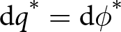 $\mathrm{d}q^* = \mathrm{d}\phi^*$. Consequently, the total differential of
 $d^*$ can be expressed as:
 \begin{equation}
\mathrm{d}d^* = \left[\frac{\alpha^* b}{q^*} \left(1 - \frac{\phi^*}{q^*}\right) + \bar{e}\right] \mathrm{d}q^*.
\end{equation}
Given that 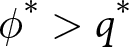 $\phi^* \gt q^*$, it follows that
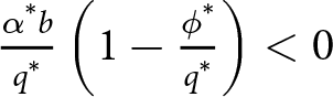 $\frac{\alpha^* b}{q^*} \left(1 - \frac{\phi^*}{q^*}\right) \lt 0$. The sign of
 $\mathrm{d}d^*$ depends on the relative magnitude of the per-capita natural resource endowment,
 $\bar{e}$, and the term
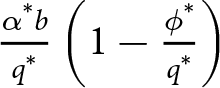
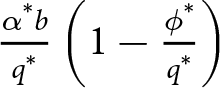 $\frac{\alpha^* b}{q^*} \left(1 - \frac{\phi^*}{q^*}\right)$. If
 $q^*$ is significantly less than
 $\phi^*$, retirees are more likely to lease quotas to active producers, risking overexploitation of the natural resource. Indeed,
 $q^*$ being small, the expression
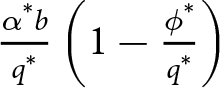 $\frac{\alpha^* b}{q^*} \left(1 - \frac{\phi^*}{q^*}\right)$ will be large enough so that
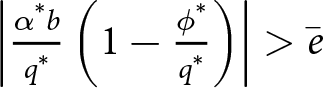 $\left| \frac{\alpha^* b}{q^*} \left(1 - \frac{\phi^*}{q^*}\right) \right| \gt \bar{e}$. In this case,
 $\mathrm{d}d^*$ becomes negative, meaning a reduction in
 $q^*$ and
 $\phi^*$ (driven by an increase in
 $\lambda^*$) increases retirees’ consumption
 $d^*$ while depleting the resource.
In a realistic scenario where  $q^*$ is close to
 $\phi^*$, retirees are less inclined to lease quotas for immediate production, promoting resource sustainability. If
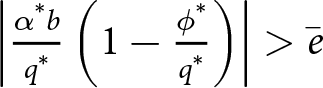 $\left| \frac{\alpha^* b}{q^*} \left(1 - \frac{\phi^*}{q^*}\right) \right| \gt \bar{e}$, reduced
 $q^*$ and
 $\phi^*$ increase
 $d^*$ while preserving the resource. However, in this case, the probability that
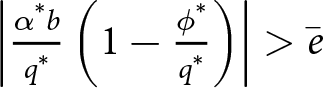 $ \left| \frac{\alpha^* b}{q^*} \left(1 - \frac{\phi^*}{q^*}\right) \right| \gt \bar{e} $ is lower, as the magnitude of the term
 $ \frac{\alpha^* b}{q^*} \left(1 - \frac{\phi^*}{q^*}\right) $ diminishes. Conversely, when
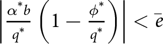 $\left| \frac{\alpha^* b}{q^*} \left(1 - \frac{\phi^*}{q^*}\right) \right| \lt \bar{e}$, reduced
 $q^*$ and
 $\phi^*$ decrease
 $d^*$ but safeguard the resource.
The analysis highlights the dual adverse effects of an increase in the shadow price of the credit constraint ( $\lambda^*$) on individual well-being and environmental sustainability. On the one hand, a rise in
 $\lambda^*$ can lead to a reduction in quota (
 $q^*$) and input (
 $\phi^*$) prices, thereby increasing retirees’ consumption (
 $d^*$) but exacerbating the overexploitation of the renewable resource. On the other hand, under certain conditions, the same reduction in
 $q^*$ and
 $\phi^*$ decreases individual consumption, harming their well-being while still contributing to resource depletion.
The results reveal a suboptimal equilibrium under binding credit constraints (non-separable case), where the individual market for transferable quotas alone is insufficient to ensure environmental preservation without compromising individual well-being.
A comparison can be made between the competitive equilibrium and the centralized economy equilibrium, which represents the social optimum. The equilibrium of the centralized economy corresponds to the point of tangency between the social utility curve and the production possibility curve, that is, an allocation of resources that ensures maximum satisfaction of all economic agents. By comparing this social optimum with the long-term competitive equilibrium, it becomes feasible to assess any divergences between the individual decisions of economic agents and the collective interest.
4.4. Financial policy, credit constraints and equilibrium trade-offs
To analyse the impact of public policy on the constrained steady state, intervention is modelled as an expansion of the effective borrowing limit:
 \begin{equation}
B_{\mathrm{eff}} = B + S_t.
\end{equation}
Here, 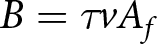 $B = \tau v A_f$ captures the collateral value, reflecting either institutional improvements such as land titling (
 $v$) or exogenous increases in land prices (
 $\tau$), while
 $S_t$ represents direct credit subsidies or guarantees. The policy mechanism operates directly through the shadow price of credit,
 $\lambda_t$, which represents the marginal utility gain from relaxing the constraint established in (45). An increase in
 $B_{\mathrm{eff}}$ necessarily reduces this shadow price,
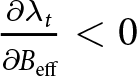 $\frac{\partial \lambda_t}{\partial B_{\mathrm{eff}}} \lt 0$, narrowing the financial wedge observed in the modified no-arbitrage condition (36),
 $\phi_t = f_{e_t}(k_t, e_t) \left( \frac{U_{c_t}(\cdot)}{U_{c_t}(\cdot) + \lambda_t} \right)$.
As  $\lambda_t$ tends to 0, the effective resource price
 $\phi_t$ converges to its marginal product
 $f_{e_t}(\cdot)$, restoring the efficiency conditions of the unconstrained competitive equilibrium. Because the constraint initially induces underutilization of the resource relative to its profitable scale, relaxing it increases the optimal resource input
 $e_t$.
However, this efficiency gain introduces a transitional environmental trade-off. From the resource law of motion in (41), the short-run impact of financial relaxation – whether through direct subsidies ( $S_t$), land titling reforms (
 $v$) or land value appreciation (
 $\tau$) – on the resource stock is negative along the transition. Specifically, for any policy instrument
 $z \in \{S_t, v, \tau\}$, the effect is:
 \begin{equation}
\frac{\partial X_{t+1}}{\partial z} = \underbrace{\frac{\partial X_{t+1}}{\partial e_t}}_{-N} \times \underbrace{\frac{\partial e_t}{\partial z}}_{ \gt 0} \lt 0.
\end{equation}
Relaxing credit constraints improves allocative efficiency, but it also creates a short-run environmental trade-off. Because producers move towards the efficient resource scale, extraction initially rises, and the resource stock falls during the transition.
In the long run, however, a sufficiently robust relaxation of credit frictions allows the steady-state allocation to converge towards the unconstrained competitive equilibrium. Since the constrained steady-state stock  $X^{*NS}$ typically falls below the unconstrained level
 $X^{*S}$ (as established in Sections 4.3 and 4.5), such policies ultimately support a higher sustainable long-run stock, consistent with the social optimum characterized in the absence of financial frictions.
The implementation of  $S_t$ is not costless. Financing these interventions through a lump-sum tax on the young generation reduces disposable income and contemporaneous consumption
 $c_t$, as shown in the budget constraint (43). Thus, the gain in allocative efficiency must be balanced against the welfare loss from financing. Policymakers must therefore weigh the fiscal requirements against the anticipated long-term gains in welfare and the stability of the sustainable resource stock.
4.5. Central planner problem
The central planner seeks to maximize aggregate welfare subject to resource constraints and natural resource sustainability, independent of price considerations. To achieve this, the central planner selects the optimal levels of consumption, capital and environmental quality. Formally, the central planner’s problem is expressed as:
 \begin{align*}
\underset{c, \ell, d, X, k, e}{\max} \quad & W = N \{U(c, \ell; X) + \beta U(d, X)\}\\
\text{s.t} \quad & Nc + Nd + Nk = F(Nk, N\bar{e}, N)\\
& G(X) = N\,\bar{e},
\end{align*}
which can be written, by substituting the constraints into the objective equation, as:
 \begin{equation}
\underset{ k, d, X}{\max} \quad W = N \left\{U \left(\frac{1}{N}F(Nk, G(X), N) - d - k, \ell; X \right) + \beta U(d, X)\right\}.
\end{equation}
The socially optimal capital stock coincides with the steady-state competitive equilibrium (48), as derived from the FOC for  $k$:
 \begin{equation}
F_K(\cdot) = 1.
\end{equation}
Similarly, the intertemporal marginal rate of substitution that ensures the welfare of all coincides with that found in long-term competitive equilibrium in (54). It follows from the FOC with respect to consumption of retirees  $d$:
 \begin{equation}
U_{c}(\cdot) = \beta U_{d}(\cdot).
\end{equation}
This relationship links consumption and savings choices over time.
The optimal level of exploitable resource ( $X^{\#}$) while ensuring biomass sustainability for future generations is derived from the FOC relative to the biomass stock
 $X$:
 \begin{equation}
\frac{U_{X}(\cdot)}{U_{d}(\cdot)} = - F_{E}(\cdot) \frac{G^{'}(X^{\#})}{N}.
\end{equation}
Compared to Equation (52), this condition shows that the social optimum takes into account, in addition to the net recruitment of the stock, the production technology in determining the level of exploitable resource. This optimal level differs from that which prevails in competitive equilibrium, where economic agents do not consider the impact of their consumption on environmental quality.Footnote 7
The optimal level of exploitable resource can be decentralized through a transferable quota policy, where the price  $ q^* $ is derived by combining (56) and (59) with (67):
 \begin{equation}
q^* = F_{E}(\cdot) \left[\frac{U_{c}(\cdot)}{U_{c}(\cdot) + \lambda} + \frac{G^{'}(X^{\#})}{N} \right] = F_E(\cdot) \left(\frac{U_{c}(\cdot)}{U_{c}(\cdot) + \lambda} \right) - \frac{U_X (\cdot)}{U_d (\cdot)}.
\end{equation}
In this framework,  $ F_E (\cdot)$ denotes the marginal productivity of the natural resource in production, reflecting the direct economic value of the resource. The term
 $\frac{G'(X^{\#})}{N}$ adjusts the price of the quota to reflect the externalities of resource exploitation, representing the impact per agent on the total stock of natural resources. By internalizing these externalities, the ITQ policy incentivizes agents to account for the long-term sustainability of the resource, aligning individual behaviour with social objectives, even in non-cooperative settings. Furthermore, the ratio
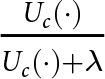 $\frac{U_c(\cdot)}{U_c(\cdot) + \lambda}$ adjusts the quota price to incorporate credit constraints, indicating that agents facing borrowing limitations (
 $\lambda \gt 0$) experience reduced marginal utility from available consumption.
By aligning individual incentives with social objectives, the ITQs market helps achieve an equilibrium where agents’ resource decisions support sustainability. The price mechanism,  $q^*$, integrates the economic value of the resource, the impact of exploitation and the credit constraints of the agents, forming a comprehensive pricing mechanism that internalizes non-cooperative behaviours and supports a socially optimal long-term equilibrium. This policy not only promotes efficient resource allocation based on agents’ preferences and opportunity costs, but also incentivizes conservation and allows agents to benefit from future environmental gains, thereby aligning private and social interests in natural resource use.
In the absence of credit constraints ( $\lambda = 0$), the equilibrium aligns with Jouvet and Rotillon (Reference Jouvet and Rotillon2005), where the quota price fully reflects the marginal productivity of the resource. This leads to a Pareto-optimal allocation, maximizing the economics, environmental and social welfare without the possibility of improving one without harming another. Resource use decisions are aligned with long-term sustainability, incentivizing agents to internalize both economic and environmental values.
However, when  $\lambda \gt 0$, binding credit constraints introduce Pareto inefficiency. The marginal utility of consumption is lower for credit-constrained agents, distorting the quota price and preventing the decentralized equilibrium from achieving social optimality. In this case, economic welfare can be improved without reducing the environmental welfare, demonstrating the inefficiency of the equilibrium with
 $\lambda \gt 0$.
To restore Pareto optimality, public policies aimed at improving access to credit are necessary. By eliminating credit constraints (setting  $ \lambda = 0 $), such policies, such as loan guarantees or subsidies for low-income households, would allow agents to fully exploit the resource in accordance with its marginal productivity and sustainability requirements. This would result in a socially optimal equilibrium where both private and social interests in resource use are aligned, and resource allocation is efficient across all agents.
4.6. Numerical illustration
A calibrated numerical illustration of these analytical results – specializing the model to Cobb–Douglas production, logistic resource growth and logarithmic preferences – is provided in the accompanying online appendix. Consistent with the analysis above, it shows that under a binding credit constraint, the resource price reflects only about half of its marginal product (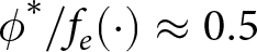 $\phi^*/f_e(\cdot)\approx 0.5$), while the real steady-state allocation (
 $k^*$,
 $y^*$,
 $c^*$,
 $d^*$,
 $X^*$) is pinned down by the government quota and is therefore invariant to the credit regime. A modest expansion of the effective borrowing limit removes the price wedge and restores the efficient ITQ outcome of Jouvet and Rotillon (Reference Jouvet and Rotillon2005). Full functional forms, calibration (Table A1), scenario results (Table A2) and the accompanying figure (Figure A1) are reported in the online appendix.
5. Conclusion
This paper examines the effectiveness of ITQs in supporting sustainable resource management within an OLG economy where agricultural producers face credit constraints. Three main results emerge.
First, absent credit frictions, the ITQ system restores the social optimum by internalizing both the externalities of natural-resource use and those arising from non-cooperative quota markets, extending Jouvet and Rotillon (Reference Jouvet and Rotillon2005) to an economy of agricultural households that are simultaneously producers and consumers. Second, when credit markets are imperfect, ITQs alone are insufficient: the constraint creates a wedge, captured by the shadow price  $\lambda_t$, between the resource price
 $\phi_t$ and its marginal product, disrupting separability and preventing the decentralized equilibrium from achieving social optimality. Third, public policies that improve credit access are therefore necessary complements to ITQ systems; as the online appendix illustrates, a modest intervention that raises the effective borrowing limit to the threshold eliminates the wedge at modest fiscal cost, while the environmental cost of credit relaxation is mainly transitional.
The analysis has several limitations that point towards future work. The model relies on an exogenous collateral constraint and abstracts from financial accelerator effects (Bernanke and Gertler, Reference Bernanke and Gertler1986; Kiyotaki and Moore, Reference Kiyotaki and Moore1997), heterogeneous credit access and endogenous debt dynamics. Embedding the present framework into a dynamic stochastic general equilibrium model would allow the study of aggregate shocks, reform sequencing and formal welfare comparisons across policy regimes. On the empirical side, the separability condition at the core of this analysis can be tested using the methodology of Benjamin (Reference Benjamin1992) and LaFave and Thomas (Reference LaFave and Thomas2016) applied to resource-using households under quota regulation, while quasi-experimental variation in credit access from land titling reforms offers a natural identification strategy. Such extensions would strengthen the bridge between the analytical insights developed here and the quantitative policy evaluation that resource management in developing economies requires.
Supplementary material
The supplementary material for this article can be found at 10.1017/S1355770X26100746.
Acknowledgements
This paper is based on a chapter of my PhD thesis completed at Université de Sherbrooke. I am deeply grateful to my supervisors, Antoine Gervais and Patrick Richard, as well as my committee members, Amanda Guimbeau, Jenny Aker, and Mario Fortin, for their invaluable guidance, comments and support. I also thank Kyle Emerick and Marina N. Mavungu for helpful discussions, and the editor, associate editor, and two anonymous referees for valuable comments and suggestions. I am also grateful to participants at the 2024 Congress of the Cercle des économistes congolais for useful feedback. All remaining errors are my own.
Competing interests
The author declares none.











 Open access

