



1. Introduction
Accurately characterising the statistical scaling and instantaneous structural coherence of turbulent fluctuations remains a central challenge in computational and experimental fluid dynamics, owing to incomplete flow information: numerical models incur intrinsic inaccuracies, while experimental methods are constrained by resolution limits (Duraisamy et al. Reference Duraisamy, Iaccarino and Xiao2019). For example, wall-modelled large-eddy simulations (WMLES) resolve only motions larger than the local grid scale, while approximating near-wall small-scale dynamics with Reynolds-averaged Navier–Stokes (RANS)-like models (Marusic et al. Reference Marusic, Mathis and Hutchins2010; Griffin et al. Reference Griffin, Fu and Moin2021, Reference Griffin, Fu and Moin2023) – this balances computational cost against accuracy. However, these near-wall dynamics – essential to turbulence physics – are often inaccurately represented by WMLES (Ying et al. Reference Ying, Li and Fu2024). Experimentally, while wall-pressure data are readily accessible via advanced optical diagnostics, the essential three-dimensional flow dynamics remain obscured (He et al. Reference He, Li and Liu2025). Previous studies underscore the critical role of wall-pressure gradients in vorticity generation within wall-bounded turbulence (Wang, Wang & Zaki Reference Wang, Wang and Zaki2022a; Xiang et al. Reference Xiang, Eyink and Zaki2025). This raises a key question: through which mechanisms – linear, nonlinear, or a combination thereof – do wall-pressure gradients modulate near-wall vorticity generation? One promising approach is the inverse modulation of vorticity flux through wall-pressure gradients, enabled by data assimilation (DA).
By integrating computational models with sparse experimental data, DA has emerged as a powerful approach for addressing challenges in turbulence state estimation (Duraisamy et al. Reference Duraisamy, Iaccarino and Xiao2019). Previous attempts to estimate the state of wall-bounded turbulence from limited observations can be separated into two general classes: data-driven and physics-driven (Brunton et al. Reference Brunton, Noack and Koumoutsakos2020; Zaki Reference Zaki2025). The former strategy addresses inverse problems by employing machine learning in conjunction with DA to surrogate key elements in prediction such as the forward operator (Fukami et al. Reference Fukami, Fukagata and Taira2019; Karniadakis et al. Reference Karniadakis, Kevrekidis, Lu, Perdikaris, Wang and Yang2021; Cheng et al. Reference Cheng, Liu, Guo and Arcucci2024), the transformation function (Kim et al. Reference Kim, Kim, Won and Lee2021; Wang et al. Reference Wang, Shi, Lei and Fung2022b ) and reduced-order modelling (Guëmes, Discetti & Ianiro, Reference Guëmes, Discetti and Ianiro2019; Zerfas et al. Reference Zerfas, Rebholz, Schneier and Iliescu2019). Although these data-driven strategies are powerful and efficient, they require substantial training data, and face challenges including high-order mode truncation and limited generalisation when applied to unseen flow regimes (He et al. Reference He, Li and Liu2025). By contrast, physics-driven strategies provide superior generalisability, interpretability and adherence to established physical principles (Zaki & Wang Reference Zaki and Wang2021). Crucially, they preserve the capacity to couple multi-scale processes that are essential for complex forecasting (Clark Di Leoni et al. Reference Clark Di Leoni, Mazzino and Biferale2020).
Within physics-driven DA frameworks, two primary mechanisms enable super-resolution reconstruction. The first, often termed ‘pouring time into space or vice versa’, exploits the intrinsic spatiotemporal linkage embedded in governing equations (Scarano & Moore Reference Scarano and Moore2012; Mons et al. Reference Mons, Chassaing, Gomez and Sagaut2016). Implementations include weighted forward–backward time integration (Chandramouli et al. Reference Chandramouli, Memin and Heitz2020; Wang & Zaki Reference Wang and Zaki2021), sliding-window four-dimensional variational (4DVar) DA (Li, He & Liu Reference Li, He and Liu2023b
), and weak-constraint 4DVar achieving temporal resolution beyond 20 times the Nyquist limit (He et al. Reference He, Zeng, Wang and Wen2024). The second mechanism relies on turbulence scale modulation, where small-scale structures are synchronised using the evolution of the Navier–Stokes equations (NSEs) based on large-scale flow fields (Ganapathisubramani et al. Reference Ganapathisubramani, Hutchins, Monty, Chung and Marusic2012; Fiscaletti et al. Reference Fiscaletti, Ganapathisubramani and Elsinga2015). Studies in homogeneous turbulence have shown that observing the velocity field at scales
 $k\eta \lt 0.2$
(where
 $k$
is the wavenumber, and
 $\eta$
is the Kolmogorov length scale) ensures full synchronisation – a process where a chaotic system adjusts its dynamics to match a reference state (Yoshida et al. Reference Yoshida, Yamaguchi and Kaneda2005; Lalescu et al. Reference Lalescu, Meneveau and Eyink2013; Clark Di Leoni et al. Reference Clark Di Leoni, Mazzino and Biferale2020; Vela-Martín Reference Vela-Martín2021). However, Wang & Zaki (Reference Wang and Zaki2021, Reference Wang and Zaki2022), who conduct the first synchronisation for wall-bounded turbulence in physical space, propose that the Taylor microscale would be more appropriate to quantify the threshold. Although synchronisation thresholds offer theoretical guidance for velocity-based DA, their applicability to wall-bounded turbulence is limited by the need for highly resolved velocity data and the central role of near-wall vorticity flux generation.
Wall-pressure measurements, intimately linked to the wall-normal vorticity flux governing near-wall dynamics, offer a compelling alternative observable. Physics-driven methods – including Kalman filters (Hœpffner et al. Reference Hœpffner, Chevalier, Bewley and Henningson2005; Chevalier et al. Reference Chevalier, Hæpffner, Bewley and Henningson2006), linear stochastic estimation (Suzuki & Hasegawa Reference Suzuki and Hasegawa2017; Encinar & Jiménez Reference Encinar and Jiménez2019) and 4DVar (Bewley & Protas Reference Bewley and Protas2004; Wang & Zaki Reference Wang and Zaki2021) – can achieve good accuracy in the regions less than 20 wall units. However, reconstruction accuracy deteriorates rapidly beyond the buffer layer due to inherent challenges: global sensitivity demands prohibitively long observation times, while adjoint-based formulations suffer from ill-conditioned Hessians and Lyapunov divergence, restricting assimilation windows (Wang et al. Reference Wang, Wang and Zaki2022a). Computational costs further compound these issues, as full-domain adjoint integrations over large time horizons remain intractable (Gronskis, Heitz & Mémin Reference Gronskis, Heitz and Mémin2013; Zaki & Wang Reference Zaki and Wang2021). While cost-reduction strategies such as coarse meshes or weak constraints have been attempted, they risk cross-talk errors and reconstruction failure (He et al. Reference He, Zeng, Wang and Wen2024). Conversely, sequential approaches optimised for short integration horizons are inherently local, confining corrections to regions adjacent to wall observations (He et al. Reference He, Liu and Gan2020). Pressure-based methods exploit pressure–velocity coupling to propagate corrections through the pressure Poisson equation. However, the interaction between localised pressure forcing and autonomous turbulence regeneration remains poorly understood, particularly regarding the influence of sensor coverage. Addressing this gap is key to developing reconstruction frameworks that combine accuracy, computational efficiency and physical insight into turbulence self-sustenance.
Focusing on the dynamic modulation of vorticity flux by wall-pressure footprints, this study introduces a continuous DA framework for flow reconstruction from wall-pressure observations. Unlike conventional 4DVar methods, the algorithm partitions the adjoint system into localised subdomains and time segments, allowing efficient gradient computations within observation neighbourhoods. Crucially, we avoid global backward integration by embedding an adjoint-derived source term directly into the pressure Poisson equation. This leverages the intrinsic pressure–velocity coupling to propagate wall-driven corrections across the flow, thereby enabling localised pressure data to modulate momentum transfer and vorticity generation – key processes for reconstructing turbulence physics. The framework is evaluated across two benchmarks. First, laminar vortex shedding past a square cylinder, where reference data from a dense mesh compare coarse-mesh simulations with and without DA, assesses the dynamic response of vortex shedding establishment and accuracy of shedding frequency prediction. Second, three-dimensional turbulent flow over an NACA0012 aerofoil at a
 $12^{\circ }$
angle of attack uses synthetic pressure-sensitive paint data derived from high-fidelity large-eddy simulations (LES). The benchmark demonstrates that wall-pressure observations are sufficient to reconstruct essential statistical features, including Reynolds stresses and spectral signatures. Systematic variation of sensor coverage further reveals how the spatial localisation of pressure data influences the fidelity of vorticity flux modulation, offering new insight into the causal link between near-wall pressure gradients, momentum redistribution, and the self-sustaining dynamics of wall turbulence.
2. Methods
This section details the methodology for reconstructing unsteady turbulent flow fields from wall-pressure data. Subsection 2.1 introduces the traditional sequential adjoint-based assimilation framework applied to the momentum equations (He et al. Reference He, Liu and Gan2020). Subsection 2.2 presents the sequential adjoint-based modulation approach formulated within the pressure equation. To address numerical instabilities inherent in such reconstructions, § 2.3 describes the Tikhonov–Sobolev regularised multi-scale spectral stabilisation technique within the DA procedure. Subsection 2.4 specifies the iterative framework for both approaches.
Starting from wall-pressure observations only, we seek to evaluate an estimate of the true flow state. Traditional efforts focus on the interpretability of wall pressures using adjoint-variational DA (i.e. 4DVar): the estimation problem is cast as a constrained optimisation task, where the goal is to identify the initial condition whose nonlinear NSEs most accurately reproduce all available observations. The adjoint-based DA formulation is derived from the time-dependent NSEs:
 \begin{align}\mathcal{R}(\boldsymbol{q})=\left\{\begin{array}{c} \partial _{i}u_{i}\\[6pt] \partial _{t}u_{i}+u_{\kern-1pt j}\partial _{\kern-1pt j}u_{i}+\dfrac{1}{\rho }\partial _{i}p-\nu \partial _{\kern-1pt j}\partial _{\kern-1pt j}u_{i} \end{array}\right\}=\mathbf{0},\quad u_{i}| _{t=0}=u_{i,0}.\end{align}
Here,
 $\boldsymbol{q}$
is the state vector composed of the velocity
 $u_{i}$
and pressure
 $p$
,
 $\nu$
is kinematic viscosity, and
 $u_{i,0}$
is the initial state, the target of reconstruction. Discrepancies between model predictions and the available observations define the cost function to be minimised.
Conventional unsteady adjoint-based methods require forward integration of the primary equations and backward integration of the adjoint system over time. The outcome of the forward-adjoint loop is the gradient of the cost function, which is then used in a gradient-based optimisation process. However, this procedure requires multiple forward and backward cycles, resulting in excessive memory usage, as the primary state at each time step is needed for the backward evolution (Li et al. Reference Li, Zhang, Dong and Abdullah2020). Moreover, the cost function landscape can be highly non-convex, with numerous local minima, which limits the applicability of this method in synchronising the estimated state with the true trajectory – especially at high Reynolds numbers (Wang & Zaki Reference Wang and Zaki2021; Zaki & Wang Reference Zaki and Wang2021). To alleviate the computational and memory demands, we reformulate the assimilation strategy to operate within a reduced temporal window spanning a single time step in which observations are available, rather than across extended durations. This localised-in-time approach gives rise to two assimilation formulations: momentum-adjoint forcing (MAF), which introduces pressure-correcting forces into the momentum equation, and pressure-adjoint source (PAS), which propagates pressure adjustments via a scalar source in the Poisson equation.
2.1. Sequential adjoint-based assimilation in the momentum equation
The MAF strategy introduces a spatially varying feedback forcing term
 $F_{i}$
into the momentum equations to constrain the resolved flow dynamics. In the present implementation, the governing equations are solved within an LES framework, such that the state variables represent filtered quantities, and the effects of unresolved scales are modelled through a subgrid-scale (SGS) closure. The resulting formulation reads
 \begin{align}\mathcal{R}(\boldsymbol{q})=\left\{\begin{array}{c} \partial _{i}\tilde{u}_{i}\\[6pt] \partial _{t}\tilde{u}_{i}+\tilde{u}_{\kern-1pt j}\partial _{\kern-1pt j}\tilde{u}_{i}+\dfrac{1}{\rho }\partial _{i}\tilde{p}-\partial _{\kern-1pt j}\left[\big(\nu +\nu _{\textit{sgs}}\big)\partial _{\kern-1pt j}\tilde{u}_{i}\right]-F_{i} \end{array}\right\}=\mathbf{0}.\end{align}
Here, tildes denote filtered variables, and
 $\nu _{\textit{sgs}}$
is the SGS eddy viscosity computed using the dynamic model proposed by Germano et al. (Reference Germano, Piomelli, Moin and Cabot1991) and later modified by Lilly (Reference Lilly1992). The dynamic SGS model provides a physically motivated implicit filtering and dissipation at unresolved scales by selectively damping high-wavenumber disturbances through an eddy-viscosity mechanism. This implicit regularisation stabilises the forward and adjoint dynamics on coarse meshes by preventing unphysical energy accumulation at the grid scale, as will be demonstrated in § 2.3. We emphasise that this filtering arises from the chosen LES formulation and is not an intrinsic requirement of the MAF concept, which is defined solely by the introduction of the feedback forcing term
 $F_{i}$
. Similar scale-selective regularisation could, in principle, be achieved through alternative filtering strategies, such as scale-restricted assimilation of direct numerical simulations (DNS) data. The force term
 $F_{i}$
serves as a modulation that assimilates observations into the numerical model. This formulation shares conceptual similarities with nudging techniques (Zauner et al. Reference Zauner, Mons, Marquet and Leclaire2022), where a feedback term is added to steer the solution towards observations. However, the present method avoids the challenges associated with selecting a nudging coefficient by automatically determining the optimal correction through an adjoint loop. The DA procedure involves finding the optimal forcing term
 $F_{i}$
by minimising the cost function
 $\mathcal{J}$
, which quantifies the discrepancy between the predicted and observed states:
 \begin{gather}\mathcal{J}=\frac{\xi _{u}}{2}\int _{\mathcal{T}}\|\mathbb{H}(\boldsymbol{q})-\boldsymbol{Y}\|^{2}\,\textrm{d}\mathcal{T}\,\delta t+\frac{\zeta }{2}\int _{\mathcal{M}}\|\boldsymbol{\nabla }\boldsymbol{F}\|^{2}\,\textrm{d}\mathcal{M}\,\delta t, \nonumber \\[5pt]\text{s.t.}\quad\mathcal{R}\left(\tilde{u}_{i},\tilde{p},F_{i}\right)=0. \end{gather}
Here,
 $\mathbb{H}$
denotes the observation operator (e.g. extracting wall pressure on the observation boundary
 $\mathcal{T}$
), and
 $\boldsymbol{Y}$
represents the corresponding pressure observations. The domain
 $\mathcal{M}$
denotes the full computational region over which the forcing
 $\boldsymbol{F}$
is defined. The symbol
 $\delta t$
refers to the local time step, which is determined based on the Courant number. The dimension converter
 $\xi _{u}$
is introduced to ensure dimensional consistency between the misfit and regularisation terms, and is set to unity throughout this study. The second term in (2.3) is the Tikhonov–Sobolev regularisation term, weighted by
 $\zeta$
, which penalises spatial gradients of the source term, and enforces smoothness of the inferred forcing. Physically,
 $\zeta$
controls the smallest flow structures at which the assimilation can act: larger values of
 $\zeta$
strongly suppress high-wavenumber, rapidly varying corrections, whereas smaller values permit finer-scale forcing variations. In this sense,
 $\zeta$
defines an effective assimilation filter scale by penalising short-wavelength corrections. As shown in § 2.3, an appropriate choice of
 $\zeta$
leads to a well-conditioned Hessian and enables stable multi-scale flow reconstruction. The value of
 $\zeta$
is guided by the flow’s advection–diffusion balance (2.25), ensuring that the regularisation damps dynamically insignificant small scales without degrading physically meaningful structures.
By introducing the Lagrange multipliers, we can obtain the following relaxation optimisation problem:
 \begin{align}\mathcal{L}\left(\boldsymbol{q},\tilde{u}_{i}^{*},\tilde{p}^{*},F_{i}\right)=\mathcal{J}+\int _{\mathcal{M}}\left\langle \left(\tilde{u}_{i}^{*},\tilde{p}^{*}\right),\mathcal{R}\left(\tilde{u}_{i},\tilde{p},F_{i}\right)\right\rangle \textrm{d}\mathcal{M}\,\delta t,\end{align}
where the inner product
 $\langle {\cdot },{\cdot }\rangle$
is defined over the entire domain. The Lagrangian multipliers
 $\tilde{u}_{i}^{*}$
and
 $\tilde{p}^{*}$
are the adjoint variables corresponding to (2.2), referred to as the adjoint velocity and adjoint pressure, respectively. The optimal distribution of
 $F_{i}$
is determined by evaluating the sensitivity of the Lagrange operator
 $\mathcal{L}$
with respect to
 $F_{i}$
, while ensuring that the variations with respect to other variables vanish:
 \begin{align}\delta \mathcal{L}\equiv \delta _{{\tilde{u}_{i}}}\mathcal{L}+\delta _{\tilde{p}}\mathcal{L}+\delta _{{F_{i}}}\mathcal{L}, \delta _{{\tilde{u}_{i}}}\mathcal{L}+\delta _{\tilde{p}}\mathcal{L}=0.\end{align}
This yields the adjoint equations
 \begin{align}-\partial _{t}{\tilde{u}_{i}}^{*}+\tilde{u}_{\kern-1pt j}^{*}\partial _{i}\tilde{u}_{\kern-1pt j}-\tilde{u}_{\kern-1pt j}\partial _{\kern-1pt j}{\tilde{u}_{i}}^{*}+\frac{1}{\rho }\partial _{i}\tilde{p}^{*}-\big(\nu +\nu _{\textit{sgs}}\big)\boldsymbol{\nabla} ^{2}\tilde{u}_{i}^{*}=0,\quad \partial _{i}{\tilde{u}_{i}}^{*}=0,\end{align}
with terminal condition at
 $t=t_{0}$
:
 \begin{align}\tilde{u}_{i}^{*}(x_{i},t_{0})=0.\end{align}
Boundary conditions are enforced to cancel boundary integrals. For inflow and wall boundaries,
 \begin{align}\tilde{u}_{\tau }^{*}=0,\quad \tilde{u}_{n}^{*}=-\frac{\partial \mathcal{J}}{\partial p},\quad n_{i}\partial _{i}\tilde{p}^{*}=0,\end{align}
where
 $n_{i}$
is the unit normal vector to the surface, and the subscripts
 $n$
and
 $\tau$
denote the normal and tangential components, respectively. For the outflow boundary, where the Neumann condition is used for the primary variables, the adjoint boundary conditions are given by
 \begin{gather}\tilde{u}_{n}\cdot\tilde{u}_{\tau }^{*}+\big(\nu +\nu _{\textit{sgs}}\big)\left(n_{i}\partial _{i}\tilde{u}_{\tau }\right)=0, \nonumber\\[4pt] u_{n}\cdot\tilde{u}_{n}^{*}+\big(\nu +\nu _{\textit{sgs}}\big)\left(n_{i}\partial _{i}\tilde{u}_{n}\right)-\tilde{p}^{*}=0. \end{gather}
The tangential component of the adjoint velocity is highly sensitive to the primary velocity, which induces serious instability in the adjoint equation. Fortunately, the contribution of the outflow boundary to the adjoint flow field is rather small (Li et al. Reference Li, He and Liu2023b
). Therefore, the zero-tangential component of the adjoint velocity is applied to the outflow boundary, which significantly improves the numerical stability without deteriorating the results. When the state and adjoint equations are satisfied, the sensitivity of
 $\mathcal{L}$
to
 $F_{i}$
is
 \begin{align}\frac{\text{d}\mathcal{J}}{\text{d}F_{i}}=\frac{\partial \mathcal{L}}{\partial F_{i}}=-\tilde{u}_{i}^{*}-\zeta \partial _{\kern-1pt j}\left(\partial _{\kern-1pt j}F_{i}\right)\!.\end{align}
The Sobolev gradient regularisation acts as a Laplacian filter to smooth sharp fluctuations in
 $F_{i}$
. Full derivations are detailed in Li et al. (Reference Li, He, Peng and Liu2025). The regularisation hyperparameter
 $\zeta$
is tuned via the procedure described in § 2.3.
As is standard in variational DA formulations (Wang et al. Reference Wang, Wang and Zaki2019; Brenner et al. Reference Brenner, Piroozmand and Jenny2022; Plogmann et al. Reference Plogmann, Brenner and Jenny2024; Li et al. Reference Li, He, Peng and Liu2025), the forcing term
 $F_{i}$
is constrained to be divergence-free to ensure well-posedness of the inverse problem. This constraint is enforced at each optimisation step via a Helmholtz decomposition:
 \begin{align}F_{i}=-\left(\partial \varphi /\partial x_{i}+\varepsilon _{\textit{ijk}}\partial \psi _{k}/\partial x_{\kern-1pt j}\right)\!,\end{align}
where
 $\phi$
and
 $\psi _{k}$
are scalar and vector potentials. The strictly solenoidal choice corresponds to retaining only the curl term
 $-\varepsilon _{\textit{ijk}}\partial \psi _{k}/\partial x_{\kern-1pt j}$
. The pressure field, determined from the continuity constraint, naturally adjusts to enforce mass conservation, and the implementation confirms that the solenoidal forcing contributes zero to the pressure Poisson source term.
2.2. Sequential adjoint-based modulation in the pressure equation
A key limitation of the sequential approach is its locality: without backward integration over time, corrections affect only regions near the observations. This becomes especially problematic with wall-pressure-only data. To mitigate this locality while retaining a sequential formulation, we introduce the control through the projection step of a pressure-based fractional-step solver, exploiting the elliptic pressure–velocity coupling that instantaneously redistributes information throughout the domain.
Within a pressure implicit with splitting of operators type fractional-step scheme, we first advance a predicted velocity using the baseline filtered momentum equation, i.e. we do not inject any explicit forcing in the momentum predictor:
 \begin{align}\partial _{t}\tilde{u}_{i}+\tilde{u}_{\kern-1pt j}\partial _{\kern-1pt j}\tilde{u}_{i}=-\frac{1}{\rho }\partial _{i}\tilde{p}+\partial _{\kern-1pt j}\left[\big(\nu +\nu _{\textit{sgs}}\big)\partial _{\kern-1pt j}\tilde{u}_{i}\right]\!.\end{align}
Here,
 $\tilde{p}$
denotes the currently available pressure estimate. The predicted velocity is then projected onto the divergence-free subspace by solving a Poisson equation for the pressure update required to enforce incompressibility. In the proposed PAS formulation, this Poisson problem is augmented by a scalar control
 $\mathcal{S}$
:
 \begin{align}\partial _{i}\partial _{i}\tilde{p}=\partial _{i}\left[-\rho\partial _{t}\tilde{u}_{i}-\rho \tilde{u}_{\kern-1pt j}\partial _{\kern-1pt j}\tilde{u}_{i}+\rho\partial _{\kern-1pt j}\left[\big(\nu +\nu _{\textit{sgs}}\big)\partial _{\kern-1pt j}\tilde{u}_{i}\right]\right]+\mathcal{S}.\end{align}
Equation (2.13) should therefore be interpreted as the projection Poisson solve that completes the fractional-step update: the baseline term corresponds to the usual divergence of the predicted momentum flux, while
 $\mathcal{S}$
introduces an additional, spatially distributed correction only through the projection.
Two remarks are important for interpretation. First, the pressure variable in (2.12)–(2.13) denotes the same physical pressure; any distinction in the implementation reflects the predictor versus projection stage of the fractional-step update. Second, augmenting the Poisson equation by
 $\mathcal{S}$
is not a gauge change: it is equivalent to introducing a conservative (irrotational) acceleration in the projection update, which modifies the divergence-free velocity through pressure–velocity coupling; the equivalence is derived in Appendix A.
Physically, PAS leverages the fact that the Poisson operator is elliptic: a localised wall-pressure misfit induces a non-local pressure redistribution, and thus a non-local velocity correction through projection. This provides a principled mechanism to propagate wall information into the interior without introducing a free body force in the predictor, while retaining the sequential optimisation structure.
By introducing the Lagrange multiplier
 $\vartheta$
, the revised cost function and the relaxation optimisation problem become
 \begin{align}\mathcal{J}=\frac{\xi _{p}}{2}\int _{\mathcal{T}}\|\mathbb{H}(\boldsymbol{q})-\boldsymbol{Y}\|^{2}\,\textrm{d}\mathcal{T}\,\delta t+\frac{\zeta _{p}}{2}\int _{\mathcal{M}}\|\boldsymbol{\nabla }\mathcal{S}\|^{2}\,\textrm{d}\mathcal{M}\,\delta t, \\[-28pt] \nonumber \end{align}
 \begin{align} & \mathcal{L}\left(\boldsymbol{q},\vartheta ,\mathcal{S}\right) \nonumber \\ & =\mathcal{J}+\int _{\mathcal{M}}\left\langle \vartheta ,\partial _{i}\partial _{i}p-\partial _{i}\left[-\rho\partial _{t}\tilde{u}_{i}-\rho \tilde{u}_{\kern-1pt j}\partial _{\kern-1pt j}\tilde{u}_{i}+\rho\partial _{\kern-1pt j}\left[\big(\nu +\nu _{\textit{sgs}}\big)\partial _{\kern-1pt j}\tilde{u}_{i}\right]\right]-\mathcal{S}\right\rangle \textrm{d}\mathcal{M}\,\delta t. \\[0pt] \nonumber \end{align}
Here,
 $\xi _{p}$
is a weighting coefficient with value unity. The Lagrange multiplier
 $\vartheta$
serves as the adjoint variable associated with the pressure equation, and is referred to as the Poisson-based adjoint pressure. The optimal distribution of
 $\mathcal{S}$
is determined by evaluating the sensitivity of the Lagrange operator
 $\mathcal{L}$
with respect to
 $\mathcal{S}$
, while setting the total variations of
 $\mathcal{L}$
with respect to other state variables to zero:
 \begin{align}\delta \mathcal{L}\equiv \delta _{\tilde{p}}\mathcal{L}+\delta _{\mathcal{S}}\mathcal{L},\quad \delta _{\tilde{p}}\mathcal{L}=0.\end{align}
Using integration by parts, the variation involving the pressure field becomes
 \begin{align}\int _{\mathcal{M}}\vartheta \cdot \partial _{i}\partial _{i}{\delta }p{\textrm d}\mathcal{M}\delta t & = \int _{\mathcal{T}}\vartheta \cdot \left({n_{i}}\partial _{i}\delta p\right)\textrm{d}\mathcal{T}\,\delta t-\int _{\mathcal{T}}\delta p \cdot\left(n_{i}\partial _{i}\vartheta \right)\textrm{d}\mathcal{T}\,\delta t \nonumber \\ & \quad +\int _{\mathcal{M}}\delta p \cdot \partial _{i}\partial _{i}\vartheta\, \textrm{d}\mathcal{M}\,\delta t.\end{align}
This leads to the adjoint equation for
 $\vartheta$
:
 \begin{align}\partial _{i}\partial _{i}\vartheta =0.\end{align}
To eliminate boundary integrals, adjoint boundary conditions are derived. At inflow boundaries, where primary variables are prescribed, the adjoint pressure is set to zero:
 \begin{align}\vartheta =0.\end{align}
At the outflow and wall boundaries, where Neumann conditions are applied to the primary variables, the adjoint boundary condition becomes
 \begin{align}n_{i}\partial _{i}\vartheta =-\frac{\partial \mathcal{J}}{\partial p}.\end{align}
Once the state and adjoint equations are satisfied, the sensitivity of the Lagrangian with respect to
 $\mathcal{S}$
becomes independent of the change in the adjoint variables and can be computed as
 \begin{align}\frac{\text{d}\mathcal{J}}{\text{d}\mathcal{S}}=\frac{\partial \mathcal{L}}{\partial \mathcal{S}}=-\vartheta -\zeta \partial _{\kern-1pt j}(\partial _{\kern-1pt j}\mathcal{S}).\end{align}
2.3. Tikhonov–Sobolev regularised multi-scale spectral stabilisation
To analyse perturbation propagation and the associated regulation behaviour, we adopt the MAF formulation; the PAS formulation exhibits analogous dynamics and leads to the same conclusions. The governing equations are deliberately linearised about a spatially uniform base flow, rendering the linear operator translation-invariant, and eliminating mean shear effects such as critical-layer branches. The purpose of this spectral model is not to recover the full spectrum associated with a sheared base flow – such features can be obtained through a full adjoint-based analysis (Wang et al. Reference Wang, Wang and Zaki2022a ) – but to construct a physically motivated and computationally efficient regularisation strategy that addresses the intrinsic ill-posedness of the inverse problem within the present DA framework. This simplification yields an analytically tractable spectral model that exposes the mechanisms responsible for ill-conditioning and directly informs the design of a scale-selective Tikhonov–Sobolev regularisation.
Provided that the tangent linear operator
 $L=\partial \mathcal{R}/\partial \boldsymbol{q}$
is continuously differentiable and invertible at a reference solution
 $(\boldsymbol{q}_{0},F_{i,0})$
, the implicit function theorem guarantees a unique local mapping
 $\boldsymbol{q}(F_{i})$
. For an infinitesimal perturbation
 $\delta F_{i}$
, the resulting state perturbation
 $\delta \boldsymbol{q}$
satisfies
 $\delta \boldsymbol{q}=-L^{-1}\,\left.\partial \mathcal{R}/\partial F_{i}\right| _{({\boldsymbol{q}_{{0}}},{F_{i,0}})}\delta F_{i}$
. For incompressible NSEs, the forcing
 $F_{i}$
acts as an additive source in the momentum equation. As a result, the operator
 $\partial R/\partial F_{i}$
reduces to the negative identity operator, thereby simplifying the expression to
 \begin{align}\delta \boldsymbol{q}=L^{-1}\,\delta F_{i}.\end{align}
The Hessian operator
 $\mathcal{H}$
, quantifying the curvature of the unregularised cost function
 $\mathcal{J}$
, is
 \begin{align}\delta ^{2}\mathcal{J}=\left\langle \delta F_{i},\mathcal{H}\,\delta F_{i}\right\rangle ,\quad \mathcal{H}=(L^{-1})^{*}L^{-1},\end{align}
where
 $(L^{-1})^{*}$
is the adjoint inverse operator (see Appendix B for full derivation).
Using Plancherel’s theorem, the action of
 $L$
on a Fourier mode
 ${\textrm e}^{{\textrm i}\boldsymbol{kx}}$
is multiplicative:
 \begin{align}L{\textrm e}^{{\textrm i}\boldsymbol{k}x}=\hat{L}\left(\boldsymbol{k}\right){\textrm e}^{{\textrm i}\boldsymbol{kx}},\quad \hat{L}\left(\boldsymbol{k}\right)={\textrm i}\left(\omega +\tilde{\boldsymbol{u}}\boldsymbol{\cdot }\boldsymbol{k}\right)+\big(\nu +\nu _{\textit{sgs}}\big)\|\boldsymbol{k}\|^{2},\end{align}
accounting for advection (base flow convection) and diffusion (molecular and SGS). The Hessian spectrum for wavenumber
 $\boldsymbol{k}$
is
 \begin{align}\lambda \left(\boldsymbol{k}\right)=\xi _{u}\left| \hat{L}\left(\boldsymbol{k}\right)\right| ^{-2}={\xi _{u}}\left[\underset{\textit{advection}}{\underbrace{\left(\omega +\tilde{\boldsymbol{u}}\boldsymbol{\cdot }\boldsymbol{k}\right)^{2}}}+\underset{\textit{diffusion}}{\underbrace{\big(\nu +\nu _{\textit{sgs}}\big)^{2}\|\boldsymbol{k}\|^{4}}}\right]^{-1}.\end{align}
This spectrum exhibits two critical defects. As
 $\|\boldsymbol{k}\|\rightarrow \infty$
,
 $\lambda (\boldsymbol{k})\sim (\nu +\nu _{\textit{sgs}})^{-1}\|\boldsymbol{k}\|^{-4}\rightarrow 0$
, causing an unbounded condition number. The second critical issue arises from a sharp transition in the eigenvalue spectrum at intermediate wavenumbers. This spectral transition induces two problems: (i) sharp eigenvalue gradients amplify sensitivity to forcing perturbation, causing erratic convergence in medium-scale dynamics; (ii) energy accumulates at
 $k_{c}$
, generating unphysical vorticity concentrations in assimilated fields (He et al. Reference He, Liu and Gan2020; Li et al. Reference Li, He and Liu2023b
).
Tikhonov–Sobolev regularisation modifies the Hessian operator according to
 \begin{align}\mathcal{H}_{\textit{reg}}=\mathcal{H}+\zeta (-{\nabla} ^{2}),\end{align}
which yields the regularised eigenvalues
 $\lambda _{\textit{reg}}(\boldsymbol{k})=\lambda (\boldsymbol{k})+\zeta\,\|\boldsymbol{k}\|^{2}$
. This modification introduces a scale-selective response. At low wavenumbers, where advection dominates,
 $\lambda _{\textit{reg}}(\boldsymbol{k})\sim \|\boldsymbol{k}\|^{-2}$
, and the effect of regularisation is negligible. At high wavenumbers, where diffusion prevails, the spectrum behaves as
 $\lambda _{\textit{reg}}(\boldsymbol{k})\sim \zeta\,\|\boldsymbol{k}\|^{2}$
, converting the rapidly decaying eigenvalues into a controlled quadratic growth. This bounded high-wavenumber behaviour prevents energy accumulation and ensures numerical stability. In the intermediate regime, the regularised spectrum attains a minimum at a critical wavenumber
 $\boldsymbol{k}_{c}$
. By the arithmetic–geometric mean inequality,
 \begin{align}\min \big(\lambda (\boldsymbol{k})+\zeta \boldsymbol{k}^{2}\big)\geq 2\sqrt{\lambda \left(\boldsymbol{k}_{c}\right)\boldsymbol{\cdot }\zeta \boldsymbol{k}_{c}^{2}},\end{align}
with equality when
 $\lambda (\boldsymbol{k}_{c})=\zeta\,\|\boldsymbol{k}_{c}\|^{2}$
. This condition provides a natural guideline for selecting the regularisation parameter
 $\zeta$
, yielding
 \begin{align}\zeta \,\|\boldsymbol{k}_{c}\|^{2}=\xi _{u}\left[\left(\omega +\tilde{\boldsymbol{u}}\boldsymbol{\cdot }\boldsymbol{k}_{c}\right)^{2}+\big(\nu +\nu _{\textit{sgs}}\big)^{2}\,\|\boldsymbol{k}_{c}\|^{4}\right]^{-1}.\end{align}
Invoking Taylor’s frozen turbulence hypothesis
 $\omega =-\tilde{\boldsymbol{u}}\boldsymbol{\cdot }\boldsymbol{k}_{c}$
(Taylor Reference Taylor1938), the advective contribution vanishes, leading to
 \begin{align}\zeta \big(\nu +\nu _{\textit{sgs}}\big)^{2}\|\boldsymbol{k}_{c}\|^{6}=\xi _{u}.\end{align}
An analogous spectral analysis applies to the PAS strategy. There, the state variable
 $\boldsymbol{q}$
is constrained by the pressure Poisson equation with source term
 $\mathcal{S}$
. Linearisation yields
 $\delta \boldsymbol{q}=\mathcal{G}^{-1}\,\delta \mathcal{S}$
, with spectral symbol
 $\hat{\mathcal{G}}(\boldsymbol{k})=\hat{L}(\boldsymbol{k})\,\|\boldsymbol{k}\|^{2}$
. The corresponding Hessian eigenvalues satisfy
 $\lambda (\boldsymbol{k})=\xi _{p}\,| \hat{\mathcal{G}}(\boldsymbol{k})| ^{-2}$
, leading to the regularisation guideline
 \begin{align}\zeta _{p}\big(\nu +\nu _{\textit{sgs}}\big)^{2}\|\boldsymbol{k}_{c}\|^{10}=\xi _{p}.\end{align}
This relation highlights that the inclusion of an SGS viscosity within the DA framework provides an inherent regularising effect, coupling the regularisation strength directly to the dissipative scale of the flow.
2.4. Iterative framework
The iterative optimisation procedures for both momentum correction
 $F_{i}$
and pressure correction
 $\mathcal{S}$
follow a consistent mathematical framework. The correction term
 $\mathcal{C}$
(where
 $\mathcal{C}=F_{i}$
for momentum-based modulation, or
 $\mathcal{C}=\mathcal{S}$
for pressure-based modulation) is updated iteratively through
 \begin{align}\mathcal{C}^{l+1}=\mathcal{C}^{l}+\alpha g_{l},\end{align}
where
 $l$
denotes the iteration index,
 $\alpha$
is the step size determined by the optimisation strategy, and
 $g_{l}$
represents the search direction. Two gradient-based strategies are employed to compute
 $g_{l}$
. The steepest descent utilises the negative sensitivity gradient scaled by an adaptive step size:
 \begin{align}g_{l}=-\partial \mathcal{L}/\partial \mathcal{C},\quad \alpha =\frac{\lambda }{\max (\partial \mathcal{L}/\partial \mathcal{C})},\end{align}
where
 $\lambda$
is a scaling factor derived from the first primary-adjoint iteration (He et al. Reference He, Liu and Gan2020). The nonlinear conjugate gradient accelerates convergence by incorporating historical gradient information via the Fletcher–Reeves formula:
 \begin{align}g_{l}=-\left(\partial \mathcal{L}/\partial \mathcal{C}\right)_{l}+\beta _{l} g_{l-1},\quad \beta _{l}=\frac{\|\!\left(\partial \mathcal{L}/\partial \mathcal{C}\right)_{l}\!\|^{2}}{\|\!\left(\partial \mathcal{L}/\partial \mathcal{C}\right)_{l-1}\!\|^{2}},\end{align}
with
 $\alpha$
optimised using Brent’s line search algorithm.
The iterative framework for sequential flow field reconstruction operates as follows. At each time step, the system checks for available observations. If none are available, then it advances to the next time step. If observations are available, then the adjoint equations are solved to evaluate the sensitivity of the Lagrangian function. This sensitivity information is then employed to update the force correction. Each iteration involves solving the primary and adjoint equations once, followed by an update to the correction force. The adjoint equations are derived by linearising the NSEs, yielding a linear system that is computationally less demanding than solving the primary nonlinear equations.
Compared to the momentum-equation-based approach, the pressure equation modulation offers significant advantages by embedding the adjoint-derived correction within the pressure equation. This leverages the inherent global propagation characteristics of the elliptic Poisson equation. In contrast, localised momentum corrections primarily influence velocity fields near observation points. The pressure-based adjustments implicitly redistribute information across the entire computational domain through the velocity–pressure coupling inherent in the incompressible NSEs. This broader influence helps to mitigate issues such as local minima when assimilating only wall-pressure observations. The pressure-based method also simplifies the adjoint formulation. By eliminating the need to solve momentum-like adjoint equations, it avoids the numerical instabilities associated with the convective terms present in momentum-based adjoint formulations. The resulting Poisson-based adjoint equation is more stable and computationally efficient. Solving a scalar Poisson equation for the correction is more efficient than applying a vector-valued momentum forcing. Furthermore, the absence of time derivatives in the adjoint pressure equation removes the requirement for backward time integration, significantly reducing memory overhead. These features make the pressure-based method ideal for wall-bounded flows, where pressure measurements encode critical global dynamics, achieving a broader spatial influence for corrections while maintaining robustness.
3. An oscillator flow over a square-section cylinder
Flow past a square cylinder is a canonical self-excited oscillator. For Reynolds numbers exceeding 50, the flow becomes unsteady, exhibiting a periodic limit cycle dominated by a fundamental vortex-shedding frequency and its harmonics. We first detail the configuration and numerical set-up. Then, by comparing coarse-mesh simulations – with and without DA – against reference data from a fine mesh, we assess the dynamic response during vortex-shedding establishment and the accuracy of shedding frequency prediction.
3.1. Configuration and numerical set-up
Figure 1 depicts the computational domain. The inflow boundary, located 10 diameters upstream of the cylinder centre, prescribes a uniform velocity profile aligned with the square’s lateral sides at Reynolds number
 $Re=LU_{0}/\upsilon =100$
. Symmetry conditions are imposed on the lateral boundaries, positioned 7.5 diameters from the cylinder centre, while the outflow boundary is placed 30 diameters downstream. Table 1 summarises the physical and numerical parameters. The reference flow was obtained via DNS on a uniform fine mesh using a second-order semi-implicit temporal scheme. Periodic vortex shedding commenced at 90 s during the 400 s simulation. Pressure measurements for DA were acquired from probes located at the
 $1/4$
and
 $3/4$
circumferential positions between 300 s and 400 s to exclude initial transients. A coarse mesh was then constructed, yielding force coefficients with approximately 50 % error compared to the DNS. Three 100 s simulations were performed on this coarse mesh: (i) a standard unsteady laminar simulation; (ii) a DA simulation using the MAF strategy; and (iii) a DA simulation using the PAS strategy.
Computational set-up and DA performance: (a) domain with pressure probes (grey indicates DA, blue indicates validation). Cost function convergence for (b) steepest descent and (c) conjugate gradient methods. (d) Normalised convergence history: MAF versus PAS strategies.

Figure 1. Long description
The figure contains multiple panels depicting different aspects of a computational setup and data assimilation performance. Panel A shows a sketch of the domain with pressure probes, where grey indicates data assimilation (DA) and blue indicates validation. The domain dimensions are labeled with L, 3L, 10L, 15L, and 40L. Panel B is a line graph showing the cost function convergence using the steepest descent method. The x-axis represents the iteration on a logarithmic scale from 10^0 to 10^4, and the y-axis represents the residual on a logarithmic scale from 10^-2 to 10^0. The graph shows a decreasing trend in residual with increasing iterations. Panel C is another line graph showing the cost function convergence using the conjugate gradient method. The x-axis represents the iteration from 0 to 10, and the y-axis represents the residual on a logarithmic scale from 10^-2 to 10^0. This graph also shows a decreasing trend in residual with increasing iterations. Panel D is a line graph comparing the normalized convergence history of two strategies, MAF and PAS. The x-axis represents t+ from 0 to 100, and the y-axis represents the residual on a logarithmic scale from 10^-6 to 10^0. The MAF strategy is represented by a red line, and the PAS strategy is represented by a blue line. The PAS strategy shows a more significant decrease in residual over time compared to the MAF strategy.
Numerical set-up for the simulations.

Table 1. Long description
A table summarizing physical and numerical parameters for simulations. The table has two columns: Model and Square cylinder. The Model column includes Diameter in meters, Reynolds number, Number of cells in reference mesh, Time step for reference mesh, Number of cells in coarse mesh, Time step for coarse mesh, and Observation sparsity. The Square cylinder column lists the corresponding values: 0.01 meters for Diameter, 100 for Reynolds number, 400000 cells for Number of cells in reference mesh, 0.01 for Time step for reference mesh, 23000 cells for Number of cells in coarse mesh, 0.1 for Time step for coarse mesh, and 1 for Observation sparsity.
Figures 1(b) and 1(c) illustrate the convergence trajectory during a single assimilation window for the MAF strategy (PAS exhibits similar behaviour). Both methods achieve comparable final residuals; however, the nonlinear conjugate gradient method demonstrates superior convergence rate and stability, while steepest descent exhibits slower asymptotic decay – consistent with theoretical expectations for first-order methods in non-convex optimisation. Figure 1(d) compares the normalised convergence histories for MAF and PAS. In the first cycle, significant deviation from the reference flow prevented the residual from reaching the specified convergence criterion, even with an increased iteration. In subsequent cycles, however, the residual decreased markedly at the cycle onset. This improvement stems from initialising the flow with the final state from the preceding cycle, and employing adjusted pressure observations. Crucially, the strategies diverged in their final residual levels: PAS achieved a lower residual after the third cycle, indicating minimal ongoing flow field impact on the assimilation, and suggesting system stabilisation. In contrast, the MAF strategy maintained a residual level nearly three times higher than PAS throughout the cycles.
3.2. Results and discussion
Figure 2 illustrates the temporal evolution of wake vorticity behind the square cylinder for the four simulations, using dimensionless time
 $t^{+}$
. Notably, the standard coarse simulation exhibits no vortex shedding, with a symmetric elongation of the wake throughout the simulation period. In contrast, both DA simulations develop wake asymmetry – a precursor to vortex shedding – by
 $t^{+}=10$
. By the end of the depicted period, vortex shedding is fully established in both DA cases, while the standard coarse simulation persists with symmetric wake elongation. It can further be noted from figure 2 that while DA cases employing the MAF strategy transition to vortex shedding, their recirculation zones remain elongated throughout the depicted period, resembling the standard coarse simulation. This elongation persists until
 $t^{+}\approx 40$
, after which the wake contracts, approaching the length more closely resembling that of the reference simulation. This delayed contraction can be interpreted in terms of the same dynamical mechanisms that operate in a Reynolds-number–driven bifurcation. The uncorrected coarse-grid solution behaves like an over-damped, steady attractor (analogous to the low-
 $Re$
steady state), whereas the MAF corrections provide a continuous, localised source of the modal content associated with vortex shedding. Because the injected disturbances must be amplified and convect downstream before they can reorganise the entire wake, the flow requires a finite time to leave the steady attractor and approach the shedding limit cycle; this explains why the wake remains elongated up to
 $t^{+}\approx 40$
before contracting toward the reference solution. Viewed in phase-space terms, the MAF-driven trajectory does not instantaneously reach the target attractor, but evolves along a low-dimensional path that closely follows the dominant manifold connecting the steady and periodic states (Noack et al. Reference Noack, Afanasiev, Morzyński, Tadmor and Thiele2003).
Evolution of wake vorticity comparing the reference solution (Reference), standard coarse-grid simulation (Standard), and two DA strategies (MAF and PAS) at sequential time snapshots.

Further analysis of the cylinder side pressure signals reveals key differences. The PAS strategy partially mitigates a mean pressure offset evident in the MAF case. While neither DA simulation perfectly captures the oscillation amplitude, the PAS simulation accurately reconstructs the oscillation frequency. Fourier analysis of wake pressure data (figure 3) identifies a dominant peak at 0.15 Hz in the reference simulations, corresponding to Strouhal number
 $\sim0.15$
, consistent with that of Okajima (Reference Okajima1982) for a square cylinder at
 $Re=100$
. The coarse simulation without DA exhibits only a weak spectral peak near 0.14 Hz. Although the MAF strategy produces a peak at the correct frequency (0.15 Hz), its spectral energy level remains similar to the coarse simulation, indicating insufficient assimilation influence to overcome the coarse grid’s inherent limitations. In contrast, the PAS strategy yields a frequency spectrum nearly identical to the reference simulation.
Time histories of pressure, streamwise velocity and their frequency spectra at probe points P1 and P2.

According to Menter & Egorov (Reference Menter and Egorov2010), the fundamental reason why standard coarse grid simulations fail to resolve the excitation and amplification of the instability lies in the inherent deficiencies caused by grid coarsening, which lead to excessive dissipation of the von Kármán vortices. In the assimilation process, the correction term forces the flow towards the observations, sustaining vortex-shedding instabilities by transferring energy from the model to the resolved flow. Figure 4 illustrates the temporal evolution of the correction fields for different strategies. A key distinction is the broader spatial influence of the PAS correction field compared to MAF. This is particularly marked in the initial phase, where PAS corrections operate globally across the domain, while MAF corrections remain strictly local. This behaviour originates in the mathematical foundation of PAS: the strategy leverages the intrinsic global propagation property of the elliptic adjoint equation. Adjustments to pressure implicitly facilitate information redistribution throughout the computational domain, mediated by the constitutive coupling between velocity and pressure in the incompressible NSEs. Consequently, the flow undergoes rapid transition from its initial steady state to the vortex-shedding state. In contrast, localised momentum corrections predominantly alter near-wall velocities while exerting minimal influence on flow regime transitions in wall-distal regions. This spatial limitation is directly evidenced in figure 3, where oscillations show delayed onset due to insufficient excitation. Another key observation in figure 4 is the attenuation of correction intensity as the predicted flow converges towards observations. This attenuation profile serves as a diagnostic for model capability: When the numerical model inherently reconstructs the flow field, corrections peak during initial assimilation – primarily resolving discrepancies with observations – and decay rapidly thereafter. Conversely, excessive dissipation from inadequate grid resolution limits predictive accuracy; here, corrections persist at significant magnitudes, providing sustained compensation for model-induced errors.
Time evolution of correction fields for square cylinder flow: (a)
 $\partial _{i}F_{i}$
for MAF; (b)
 $\mathcal{S}$
for PAS.

4. An amplifier flow over an aerofoil
This section addresses the more challenging case of a ‘noise-amplifier’ aerofoil flow, characterised by broadband response behaviour. Owing to the global correction properties of the PAS strategy, this reconstruction approach is employed exclusively here. The configuration is first outlined, followed by an evaluation of the reconstruction procedure.
4.1. Computational set-up
4.1.1. Generation of high-fidelity database
The high-fidelity reference database was obtained through wall-resolved LES of flow over an NACA0012 aerofoil at
 $Re=3.6\times 10^{5}$
and
 $12^{\circ}$
angle of attack. The wall-adapting local eddy-viscosity SGS model was employed, with validation against time-resolved particle image velocimetry measurements (Li et al. Reference Li, He, Ge and Liu2023a
). This enabled a fully quantitative benchmark for evaluating the DA’s reconstruction capabilities, with access to the true data at every point and resolved scale.
The computational domain employs a structured C-type grid as shown in figure 5. Periodic and freestream boundary conditions are imposed at the spanwise and outer boundaries, respectively. The domain dimensions – wake length 5
 $c$
, outer radius
 $7.3c$
, and spanwise extent
 $0.3c$
– follow the validated configuration from Ribeiro & Wolf (Reference Ribeiro and Wolf2017) for
 $Re=4.1\times 10^{5}$
. The spanwise extent was chosen to ensure that two-point correlations of velocity fluctuations decayed to zero, following Jones et al. (Reference Jones, Sandberg and Sandham2008). The LES grid spacings follow the air flow criteria of Tamaki & Kawai (Reference Tamaki and Kawai2023):
 $\Delta \xi ^{+}=\Delta \xi\, u_{\tau }/{}\nu \lt 25$
(chordwise),
 $\Delta \eta ^{+}\approx 1$
(wall-normal, at wall), and
 $\Delta z^{+}\lt 13$
(spanwise), ensuring adequate resolution of near-wall streaks. The mesh also includes at least five grid points within the region
 $\eta ^{+}\lt 10$
. The time step
 $\Delta {t}_{\textit{LES}}^{+}=\Delta t_{\textit{LES}}\,U_{0}/c=2.2\times 10^{-5}$
maintained a maximum Courant–Friedrichs–Lewy (CFL) number less than 0.5. All simulations employed an in-house code (He et al. Reference He, Liu and Yavuzkurt2018) on a grid of
 $\sim45.7$
million points.
Computational set-up. (a) Geometry schematic and cross-sectional view of the locally refined grid. (b) Instantaneous vortical structures (
 $Q=10^{4}$
) coloured by wall-normal distance. For clarity, grid lines are shown at reduced sampling rates (1 : 5 in
 $\xi$
, 1 : 4 in
 $\eta$
).

Figure 6(a) shows chordwise and wall-normal grid spacings along the upper surface in viscous wall units. A sharp reduction in chordwise spacing occurs near the leading edge at
 $x/c=0.06$
, upstream of the laminar–turbulent transition (
 $x/c\approx 0.08$
). The criterion
 $\Delta \xi ^{+}\lt 25$
is satisfied in both transitional and turbulent regions. The wall-normal spacing satisfies
 $\Delta \eta ^{+}\approx 1$
across the entire upper surface. Figure 6(b) shows spanwise correlation coefficients at
 $x/c=0.4$
and
 $0.8$
, evaluated at the height of maximum turbulent kinetic energy (TKE). The correlation coefficient converges to zero at these locations, confirming that the
 $0.3c$
spanwise extent is sufficient to avoid spurious correlations. Velocity and Reynolds normal stress profiles are further examined at a mild pressure gradient location (
 $x/c=0.42$
) over the upper surface, where the turbulent boundary layer is fully developed and attached (figures 6
c,d). Comparison with DNS data for a flat-plate turbulent boundary layer at a matched friction Reynolds number (
 $Re_{\tau }=252$
; Schlatter & Örlü Reference Schlatter and Örlü2010) shows close alignment in both mean velocity and Reynolds normal stresses. These results suggest that the grid resolution is sufficient to resolve the energetic vortices in the boundary layer, as also depicted in figure 5(b), where the instantaneous vortical structures illustrate the transition and growth of the turbulent boundary layer along the upper surface.
Computation grid statistics. (a) Grid spacings along the aerofoil upper surface in the viscous wall units. (b) Spanwise correlation
 $R_{u'u'}$
. (c) Mean chordwise velocity. (d) Reynolds normal stress in viscous wall units at
 $x/c=0.42$
. Circles denote flat-plate DNS at
 $Re_{\tau }=252$
.

4.1.2. The DA set-up
Conventional state estimation typically relies on DNS with matching grids and discretisation to eliminate numerical uncertainties (Zaki Reference Zaki2025). In contrast, our DA framework adopts a deliberately coarser mesh within the same domain (table 2), which is insufficient for standalone LES, and introduces discrepancies between the reference and assimilation models. Thus the DA process is more inclined towards a weak-constraint approach (Li et al. Reference Li, He and Liu2023b ) to account for computational uncertainties, such as subgrid model errors and discretisation errors, making it more applicable to realistic flow conditions. Rather than correcting the model itself, we focus on mitigating its adverse effects on resolved flow structures (e.g. excessive dissipation), ensuring accurate state estimation at the resolved scales.
Mesh set-up for the simulations.

Table 2. Long description
A table comparing simulation parameters and control volumes. The table has four rows and six columns. The columns are labeled Simulation, Resolution, max(Δξ+), Δξ+, max(Δη+), and Control volume (106). The rows are labeled LES, CLES, and DA-CLES. Row 1: Simulation, LES; Resolution, Fine; max(Δξ+), 20; Δξ+, 12; max(Δη+), 1; Control volume (106), 45.7. Row 2: Simulation, CLES; Resolution, Coarse; max(Δξ+), 60; Δξ+, 60; max(Δη+), 5; Control volume (106), 1.7. Row 3: Simulation, DA-CLES; Resolution, Coarse; max(Δξ+), 60; Δξ+, 60; max(Δη+), 5; Control volume (106), 1.7.
Table 3 details the DA configurations examined in this study. All cases share boundary conditions identical to those of the reference simulation, with adjoint conditions defined in § 2.2. Second-order discretisation is applied consistently to the primary-adjoint system. The DA time step is set to
 $\Delta {t}_{c}^{+}=\Delta t_{c}\,U_{0}/c=2.2\times 10^{-4}$
, ensuring a maximum CFL number less than 0.5. Synthetic observations are generated from the high-fidelity database. The primary velocity field is initialised from coarse-grid free evolution. Observations are assimilated every 25 steps.
DA cases set-up.

Table 3. Long description
The table presents various data assimilation (DA) configurations examined in a study. It consists of five rows and five columns. The columns are labeled Sections, Simulation, Mesh, Observation (x/c times z/c), and Temporal sparsity (Δt0+). The rows detail different DA cases with specific configurations. Row 1: Sections 4.2-4.3, Simulation L00, Mesh not specified, Observation [0, 1] times [-0.15, 0.15], Temporal sparsity 0.0055. Row 2: Sections 4.2-4.3, Simulation Nudging, Mesh not specified, Observation [0, 1] times [-0.15, 0.15], Temporal sparsity 0.0055. Row 3: Sections 4.2-4.3, Simulation LSE, Mesh not specified, Observation [0, 1] times [-0.15, 0.15], Temporal sparsity 0.0055. Row 4: Sections 4.2-4.3, Simulation CLES, Mesh Coarse, Observation not specified, Temporal sparsity infinity. Row 5: Sections 4.4, Simulation L30-L70, Mesh not specified, Observation [0.3, 1] times [-0.15, 0.15], Temporal sparsity 0.0055. The table compares different simulations, mesh types, observation ranges, and temporal sparsity values used in the study.
* Initialisation is acquired from coarse-grid-based free evolution.
For benchmarking, steady RANS simulations with the shear stress transport (SST) model and pure LES without DA (denoted as ‘CLES’) are performed using the same mesh. Note that resolving instability wave activation (e.g. Tollmien–Schlichting waves) and turbulence boundary-layer growth in the CLES case would require higher mesh resolution than used here (Mao et al. Reference Mao, Zaki, Sherwin and Blackburn2017). Nevertheless, it provides a relevant baseline for comparison. To assess the effectiveness of the present DA framework, we also reconstruct the velocity field from wall-pressure measurements using two established methods. The first method is a continuous-based ‘nudging’ approach (Clark Di Leoni et al. Reference Clark Di Leoni, Mazzino and Biferale2020; Zauner et al. Reference Zauner, Mons, Marquet and Leclaire2022), which incorporates a feedback gain in the pressure Poisson equation. The same observations are embedded in this method, and simulations are conducted with the same computational set-up, described by the equation
 \begin{align}\partial _{i}\partial _{i}\tilde{p}=\partial _{i}\left[-\rho\partial _{t}\tilde{u}_{i}-\rho \tilde{u}_{\kern-1pt j}\partial _{\kern-1pt j}\tilde{u}_{i}+\rho\partial _{\kern-1pt j}\left[\big(\nu +\nu _{\textit{sgs}}\big)\partial _{\kern-1pt j}\tilde{u}_{i}\right]\right]+K\left(\boldsymbol{Y}-\mathbb{H}(\boldsymbol{q})\right).\end{align}
The non-dimensional feedback gain
 $K$
is set to
 $4\times 10^{6}$
, the largest value that can be used without causing divergence for this mesh and implementation. The second method uses linear stochastic estimation (LSE) with a proper orthogonal decomposition (POD)-based variant (Discetti et al. Reference Discetti, Raiola and Ianiro2018; Encinar & Jiménez Reference Encinar and Jiménez2019). A detailed description of this method and its verification on the training set is provided in Appendix E. In all DA cases, the assimilation window spans
 $\Delta T^{+}=\Delta T\,U_{0}/c=8.25$
, during which 7500 instantaneous fields are stored. The analysis is based on the last 5000 snapshots. Additionally, by systematically varying sensor coverage, we examine how spatial localisation of pressure data governs the fidelity of vorticity flux modulation.
4.1.3. On the physical interpretation of the correction and regularisation
A central challenge in DA for turbulent flows is the selection of the regularisation coefficient
 $\zeta$
, which simultaneously influences the optimisation conditioning, the physical accuracy of the reconstructed flow, and the suppression of measurement noise through its modulation of small-scale fluctuations (see Appendix D for details). To appreciate the physical significance of
 $\zeta$
, it is instructive to consider the multi-scale nature of turbulence. In a turbulent flow, energy is injected at large, energy-containing scales, and transferred through the inertial range to progressively smaller scales until it is dissipated. In LES, the computational grid can only resolve scales larger than the filter width
 $\varDelta$
, so that motions at scales smaller than
 $\varDelta$
– the SGS motions – are unresolved. These unresolved motions represent physically meaningful turbulent fluctuations that participate in the energy cascade and contribute to the Reynolds stress tensor through the SGS stress. In the present DA framework, the regularisation coefficient
 $\zeta$
controls the effective scale separation between the resolved, assimilated turbulent motions and those that are filtered out.
The connection between the regularisation weight and turbulence scales can be interpreted through the Hessian eigenstructure. The linearised NSEs operator (2.24) embeds two fundamental turbulence time scales at each wavenumber
 $\boldsymbol{k}$
: a convective time scale
 $\tau _{conv}(\boldsymbol{k})$
, governing the advection of turbulent structures by the mean flow, and a diffusive time scale
 $\tau _{\textit{diff}}(\boldsymbol{k})$
, governing their dissipation by the effective viscosity. The Hessian eigenvalue at wavenumber
 $\boldsymbol{k}$
is determined by the competition between these two time scales (2.25): at low wavenumbers, where
 $\tau _{\textit{con}v}\lt \tau _{\textit{diff}}$
, advection dominates and the eigenvalues remain comparatively large, so the inverse problem is better conditioned; at high wavenumbers, where
 $\tau _{\textit{con}v}\gt \tau _{\textit{diff}}$
, diffusion becomes increasingly important and the eigenvalues decay, rendering the inverse problem increasingly ill-conditioned. The regularisation balance (2.28) connects
 $\zeta$
to these turbulence time scales: under Taylor’s frozen turbulence hypothesis, the balance reduces to
 $\zeta\,\|\boldsymbol{k}_{c}\|^{2}=\xi _{u}\,{\tau }_{\textit{diff}}^{2}(\boldsymbol{k}_{c})$
, suggesting that the regularisation coefficient may be related to the diffusive lifetime of turbulent structures at the cut-off wavenumber
 $\boldsymbol{k}_{c}$
. The cut-off may therefore be interpreted as lying near the wavenumber at which the Hessian changes from being predominantly advection-dominated to increasingly diffusion-dominated. In other words,
 $\zeta $
is not an arbitrary numerical parameter; it encodes the time scale information of the turbulent dissipation process at the assimilation cut-off.
Although this analysis yields a theoretical relationship between
 $\zeta$
and
 $\boldsymbol{k}_{c}$
based on Hessian conditioning arguments (2.30), the resulting estimate should be viewed as a guideline for establishing an initial value rather than a definitive prescription. The optimal regularisation weight depends critically on problem-specific factors including the resolution of the observational data, the spatial discretisation of the control variable, and the particular flow physics being assimilated. The difficulty lies in the dual role of regularisation: it (i) stabilises the ill-conditioned inverse problem by improving the Hessian conditioning, and (ii) imposes an implicit spectral filter that determines the assimilated turbulent scales. Consequently, even with theoretical guidance from (2.30), an a posteriori verification procedure is essential to ensure that the chosen
 $\zeta$
yields both numerical stability and physical accuracy.
To investigate this trade-off, we examine the DA performance across nine regularisation weights spanning the range
 $[10^{-15}, 10^{-9}]$
, corresponding to wavenumbers
 $kc$
in the range
 $[10^1, 10^3]$
. This sweep enables evaluation of convergence characteristics, spectral fidelity and spatial reconstruction quality as functions of the regularisation strength. Figure 7(a) presents the convergence histories for three regularisation coefficients:
 $\zeta _{{k_{1}}}=10^{-15}$
,
 $\zeta _{{k_{2}}}=7\times 10^{-12}$
and
 $\zeta _{{k_{3}}}=5\times 10^{-11}$
, corresponding to
 $k_{1}c = 200$
,
 $k_{2}c = 85$
and
 $k_{3}c = 65$
at the first assimilation cycle, respectively. The monotonic acceleration of convergence with increasing
 $\zeta$
is apparent: the largest regularisation weight (
 $\zeta _{{k_{3}}}$
) yields the steepest residual reduction, dropping below 10−2 within five iterations, while smaller weights require more iterations to reach comparable residual levels. This aligns with theoretical expectations: Tikhonov–Sobolev regularisation modifies the eigenvalue distribution by adding a term proportional to
 $\zeta\,\|k\|^{2}$
to each eigenvalue, lifting the smallest eigenvalues and thereby reducing the condition number of the Hessian matrix. In the high-wavenumber regime, the regularised eigenvalues scale as
 $\lambda _{\textit{reg}}(k)\sim \zeta\,\|k\|^{2}$
, flattening spectral decay and preventing round-off errors in modes associated with small eigenvalues. Larger
 $\zeta$
values improve the Hessian conditioning by bounding the smallest eigenvalue from below, which translates directly to faster convergence rates in the gradient-based optimisation algorithm.
Effect of regularisation scale on convergence and spectral fidelity: (a) convergence history of the residual; (b) minimum residual attained as a function of
 $\zeta$
; (c) angular-averaged PSD of the pressure field at
 $y^{+}=5$
; and (d) corresponding PSD of the converged scalar source
 $\mathcal{S}$
at
 $y^{+}=5$
.

However, fast convergence alone does not guarantee optimal solutions. Figure 7(b) reveals a non-monotonic relationship between regularisation strength and the minimum attainable residual. As
 $\zeta$
increases from
 $10^{-15}$
to approximately
 $10^{-11}$
, the residual decreases, stabilising the inversion against numerical noise. However, beyond this point, further increases in
 $\zeta$
lead to a rise in the residual, indicating that excessive regularisation over-penalises the control variable and degrades the fit to the data. Theoretically, the unconstrained least squares solution should yield the smallest possible residual; any regularisation necessarily increases this residual by constraining the solution space. The observed non-monotonic behaviour – where moderate regularisation actually reduces the residual compared to the near-unconstrained case – demonstrates that numerical conditioning concerns can dominate theoretical optimality in practical implementations. This finding underscores the importance of regularisation not merely as a mathematical convenience but as a numerically essential component that enables stable convergence to physically meaningful solutions.
The spectral analysis in figures 7(c) and 7(d) offers critical insight into how regularisation affects the multi-scale structure of the solution. Figure 7(c) displays the angular-averaged power spectral density (PSD) of the pressure fluctuations at
 $y^{+}=5$
, comparing the LES reference with the DA reconstructions obtained using the three representative regularisation weights. For
 $\zeta _{k_1}$
, the spectrum matches the LES reference at low and medium wavenumbers, but deviates at high wavenumbers, indicating that insufficient regularisation fails to suppress spurious energy accumulation in the poorly constrained high-wavenumber range. This energy pile-up is a direct consequence of the ill-posed inverse problem: insufficient regularisation permits amplification of components associated with small singular values, or equivalently weakly observable directions of the Hessian, which manifests as oscillatory artefacts rather than physically meaningful small-scale content (Benning & Burger Reference Benning and Burger2018). In turbulence estimation from limited observations, only flow events that materially influence the measurements can be robustly recovered, whereas scales that are weakly linked to the observations remain ambiguous (Zaki Reference Zaki2025). Because the high-wavenumber modes correspond precisely to the diffusion-dominated regime of the Hessian where eigenvalues are small, these modes are the least constrained by the observational data. In the absence of sufficient regularisation, the optimiser exploits these under-determined degrees of freedom to reduce the cost functional, populating them with energy that minimises the residual in a least squares sense, but bears no physical relation to the actual dissipation range motions. The excess high-wavenumber energy is therefore best understood as a numerical artefact of the ill-conditioned inversion – an amplification of weakly constrained small-scale components – rather than a genuine recovery of fine-scale turbulence. As the regularisation increases to
 $\zeta _{{k_{2}}}$
, the spectrum aligns closely with the LES reference across all resolved wavenumbers, demonstrating optimal regularisation that balances data fidelity and model constraints. However, further increasing
 $\zeta$
to
 $\zeta _{{k_{3}}}$
causes the spectrum to deviate, with enhanced low-wavenumber energy and a steep drop-off at high wavenumbers. This behaviour can be interpreted as an implicit spatial filtering operation: strong regularisation effectively imposes a wavenumber cut-off beyond which fluctuations are heavily damped, analogous to truncating the turbulent energy cascade at an artificially low scale.
Figure 7(d) further elucidates this scale-dependent filtering by examining the spectrum of the scalar source field at the same wall-normal location. Insufficient regularisation (
 $\zeta _{{k_{1}}}$
) results in an unphysical accumulation of high-wavenumber energy, manifested as elevated spectral levels at
 $kc\gt 50$
. This behaviour reflects spectral contamination induced by the ill-conditioned inverse problem: weakly constrained small-scale degrees of freedom absorb residual misfit and produce a spurious pile-up of energy at high wavenumbers, resulting in a non-physical spectrum (Benning & Burger Reference Benning and Burger2018). Moderate regularisation (
 $\zeta _{{k_{2}}}$
) suppresses this spurious high-wavenumber energy while preserving the physically meaningful intermediate-scale content. Excessive regularisation (
 $\zeta _{{k_{3}}}$
) over-filters the solution, removing not only spurious noise, but also physically relevant intermediate-scale structures. From a dimensional standpoint, the Tikhonov–Sobolev regularisation adds a term proportional to
 $\zeta\, \| k\| ^{2}$
to each eigenvalue of the Hessian, defining a cut-off wavenumber
 $k_{c}$
and a corresponding assimilation length scale
 $\ell_{c}=2\pi /\| k_{c}\|$
. Corrections at wavelengths shorter than
 $\mathcal{O}(\ell_{c})$
are strongly penalised, so that
 $\ell_{c}$
may be interpreted as the smallest turbulent scale that the assimilation retains. Rather than a mere numerical smoother, the coefficient
 $\zeta$
therefore acts as a scale-selection parameter. The corresponding cut-off length scale is governed by two factors: the representational capacity of the LES, and the informational content of the wall-pressure observations (Kim Reference Kim1989). The cut-off may therefore be interpreted as marking the spectral boundary beyond which model fidelity and observational information become insufficient to distinguish physically meaningful corrections from spurious ones, and its proximity to the grid spacing
 $\varDelta$
reflects the convergence of these two limits near the upper end of the resolved range.
Spatial fields in figure 8 confirm these findings. With insufficient regularisation, the scalar source field shows streak-like patterns contaminated by fine-scale, noise-like oscillations. These spurious features manifest as irregular, high-frequency spatial variations superimposed on the physically meaningful large-scale structures, and bear no resemblance to the organised near-wall turbulence structures (streaks, quasi-streamwise vortices) expected from the physics of wall-bounded turbulence. The corresponding pressure field similarly exhibits unphysical fine-scale fluctuations that are inconsistent with the known spatial coherence of pressure in turbulent boundary layers. At the opposite extreme, overly strong regularisation produces an excessively smooth scalar source field that lacks the fine-scale detail present in the reference. Near-wall streaks appear diffuse and blurred, with significantly reduced spatial gradients, indicating that the regularisation has removed the dynamically important small-scale vortical motions that sustain the near-wall turbulence cycle through the self-sustaining process of streak instability and vortex regeneration (Jiménez Reference Jiménez2018). This over-smoothing directly impacts the reconstructed pressure field, removing small-scale coherent structures characteristic of wall turbulence.
Effect of regularisation scale: (a) scalar source
 $\mathcal{S}$
distribution; (b) pressure field distribution at
 $y^{+}=5$
.

This analysis of convergence behaviour, spectral content and spatial structure reveals that Tikhonov–Sobolev regularisation functions as a scale-aware control mechanism rooted in turbulence physics. The regularisation coefficient
 $\zeta$
sets an effective cut-off wavenumber
 $k_{c}$
(equivalently, a length scale
 $\ell_{c}=2\pi /k_{c}$
), which governs the balance between numerical stability and physical fidelity. This scale-selective filtering has important implications for practical DA in turbulent flows, and the choice of
 $\zeta$
should therefore be calibrated for each problem so that the assimilated field retains the essential multi-scale structure of the turbulence while avoiding spurious small-scale corrections.
4.2. Algorithm performance: statistics of the benchmark case
Figures 9, 10, 11 and 12 provide a spatially resolved assessment of reconstruction quality by showing instantaneous fluctuation fields together with the corresponding pointwise absolute error maps. Specifically, for each quantity
 $q$
(pressure fluctuation
 $p\textrm{'}$
or spanwise velocity fluctuation
 $w\textrm{'}$
), we report the instantaneous error field
 \begin{align}\epsilon (\boldsymbol{x},t)=\left| q(\boldsymbol{x},t)-q_{\textit{ref}}(\boldsymbol{x},t)\right| ,\end{align}
where
 $q_{\textit{ref}}$
is the reference LES field at the same instant. Snapshots are shown at three representative phases: initialisation (
 $t^{+}=0$
), transition (
 $t^{+}=1.35$
), and the statistically stationary state (
 $t^{+}=2.7$
). The
 $x{-}y$
plane at
 $z/c=0$
, and the near-wall
 $x{-}z$
plane at
 $y^{+}=5$
, are used to highlight, respectively, the separation/reattachment dynamics and the near-wall multi-scale content.
Instantaneous pressure fluctuations and error distributions in the
 $x{-}y$
plane at
 $z/c=0$
.

Instantaneous pressure fluctuations and error distributions in the
 $x{-}z$
plane at
 $y^{+}=5$
.

Instantaneous spanwise velocity fluctuations and error distributions in the
 $x{-}y$
plane at
 $z/c=0$
.

Instantaneous spanwise velocity fluctuations and error distributions in the
 $x{-}z$
plane at
 $y^{+}=5$
.

For pressure fluctuations, the reference case exhibits fine-scale pressure activity associated with an attached, transitional shear layer, whereas the coarse-grid baseline develops an open separation downstream of the leading edge. The separated shear layer in CLES is dominated by large coherent structures that do not break down, consistent with the fact that the present under-resolved mesh suppresses instability-wave growth and therefore delays laminar-to-turbulent transition under an adverse pressure gradient. This failure manifests directly in the pressure-fluctuation topology and in the large errors concentrated along the separated shear layer and the near-wake region. In the DA results, wall-pressure observations are incorporated every 25 LES time steps; between updates, the flow evolves under the incompressible NSEs. Both PAS and nudging imprint an immediate near-wall pressure response already at
 $t^{+}=0$
, indicating that assimilation is active from the start. By
 $t^{+}=1.35$
, both strategies markedly suppress the spurious leading-edge separation seen in CLES, and promote reattachment. The apparent delay between the onset of assimilation and the macroscopic reattachment is therefore not indicative of ‘inactive’ DA; rather, it reflects hysteresis associated with the upstream flow history and the finite convection time of the pre-existing separated structures.
Crucially, the two strategies diverge in the fidelity of the fluctuation field after the transient. The PAS yields a pressure-fluctuation pattern that rapidly approaches the reference across most of the domain, with error maps showing a pronounced reduction by
 $t^{+}=2.7$
, including in the near-wall
 $y^{+}=5$
plane. In contrast, while nudging can reduce the wall-pressure misfit, its localised feedback forcing produces steep local pressure gradients and an over-energised fluctuation response; as time advances, this manifests as visibly amplified and distorted
 $p\textrm{'}$
structures, and a persistently larger
 $\epsilon$
away from the wall, especially once the solution enters the statistically stationary regime. The LSE results are not reported for pressure here, since LSE/extended POD (EPOD) provides a direct estimate of velocity from wall pressure; the corresponding pressure field could be obtained by post-processing via a Poisson solve, but this is beyond the present scope.
Reconstructing
 $w\textrm{'}$
is more stringent than matching wall pressure because
 $w\textrm{'}$
is not directly observed and must be recovered through pressure–velocity coupling and the subsequent nonlinear evolution. The CLES snapshots again show separated-shear-layer dynamics with large-scale, weakly broken-down structures and correspondingly large velocity errors. Both PAS and nudging recover the emergence of near-wall multi-scale motions during the transition (
 $t^{+}=1.35$
), consistent with the rapid correction of leading-edge separation observed in the pressure fields. However, the error maps clarify that ‘multi-scale activity’ alone is not sufficient: nudging tends to generate overly intense fluctuations, leaving a larger wall-normal penetration error and a poorer match to the reference fluctuation organisation at
 $t^{+}=2.7$
. The PAS, by contrast, provides a more spatially coherent correction – consistent with the elliptic, domain-wide propagation of the pressure adjustment – and therefore yields smaller
 $\epsilon$
in both planes once the flow reaches statistical stationarity. The LSE/EPOD provides a complementary, purely statistical baseline for
 $w\textrm{'}$
: it can reproduce the wall-attached, strongly wall-correlated components reasonably well, yielding small near-wall errors. However, accuracy degrades with increasing wall distance and at small scales, because detached motions leave only weak pressure footprints, and the truncated POD basis suppresses weakly correlated, low-energy fluctuations.
Figure 13(a) shows the time evolution of the normalised observation residual, which quantifies the misfit between the predicted wall pressure and the assimilated wall-pressure measurements. Three distinct behaviours are observed. In the uncontrolled coarse-grid LES, the residual departs rapidly from the reference despite identical initialisation. This behaviour reflects the fact that on the present under-resolved mesh, a free Navier–Stokes evolution does not remain on the reference attractor: following an initial transient divergence, nonlinear dynamics dominates, and the estimation error saturates at a finite level. Introducing a proportional feedback term through the nudging formulation stabilises the computation and reduces the wall-pressure misfit. A gain sweep indicates that the feedback gain is strongly constrained by numerical stability on this mesh; we therefore report results at the largest stable value
 $4\times 10^{6}$
. With this choice, the residual decreases by approximately two decades, then reaches a plateau at
 $\mathcal{O}(10^{-2})$
. This plateau demonstrates convergence of the wall-pressure constraint, but also indicates an irreducible mismatch associated with coarse-grid modelling/discretisation errors and the inherently local nature of the nudging correction. In contrast, the proposed PAS strategy yields a markedly faster and stronger reduction of the residual: the misfit decreases quasi-exponentially by approximately three orders of magnitude over
 $t^{+}\lt 2.4$
, then levels off at a lower plateau. This rapid decay indicates that the adjoint-based pressure modulation efficiently removes the transient induced by the separated initial condition, and steers the solution towards the statistically stationary state.
(a) Normalised residual trajectory. (b–d) Spanwise vorticity evolution at
 $y^{+}=5$
: (b) Reference, (c) CLES, (d) PAS. Dashed lines indicate mean convection ridges.

The spatiotemporal map confirms this transition, with the shear flow’s downstream motion manifesting as inclined contour patterns. Figures 13(b) and 13(c) illustrate distinct flow behaviours: the reference case exhibits small-scale, positively inclined propagation typical of an attached boundary layer, while the CLES show large-scale, negatively inclined propagation indicative of separation. In contrast, the DA reconstruction displays an immediate transition from the separated state to a statistical steady state, reproducing the spectral complexity of the reference. Notably, an inclined dashed line in figure 13(d) marks a time lag of
 $t^{+}=2.4$
at
 $x/c=1$
that separates the large-scale separation from subsequent small-scale propagation. Previous work (Li et al. Reference Li, He, Ge and Liu2023a
) reported that vortical structures in the separated shear layer convect at
 $0.41U_{0}$
, corresponding to a convection time of 2.4 time units – matching the observed time lag. This agreement confirms that pressure modulation initiates immediately upon observation assimilation. Such instantaneous action stems from a direct viscous force linkage: unlike flow reconstruction achieving rigorous synchronisation from forward–backward sensitivity propagation (Wang & Zaki Reference Wang and Zaki2021; Wang et al. Reference Wang, Wang and Zaki2022a
), the present DA strategy serves as a physics-informed modulator, enabling simultaneous recovery of tangential pressure gradients along the aerofoil wall. To establish a more fundamental physical basis for the proposed PAS strategy, it is instructive to examine the process from the perspective of vorticity dynamics. The generation of vorticity at a solid boundary in an incompressible flow is governed by the wall-normal vorticity flux
 $J_{n}$
, which can be expressed as (Lighthill Reference Lighthill1963)
 \begin{align}J_{n}=-\hat{\boldsymbol{\tau }}\boldsymbol{\cdot }\frac{\text{d}\boldsymbol{V}_{\!w\textit{all}}}{\text{d}t}-\frac{1}{\rho }\left(\frac{\partial p}{\partial \tau }\right)_{w\textit{all}},\end{align}
where
 $\hat{\boldsymbol{\tau }}$
denotes the unit vector tangent to the wall. Equation (4.3) shows that the wall-normal vorticity flux consists of two distinct contributions: (i) the tangential acceleration of the wall,
 $\text{d}\boldsymbol{V}_{\!w\textit{all}}/\text{d}t$
, which represents the kinematic ‘rubbing’ of a moving boundary on the fluid; and (ii) the wall-tangential pressure gradient,
 $(\partial p/\partial \tau )_{w\textit{all}}$
, which is the sole mechanism for vorticity generation at a stationary wall. For the present study concerning stationary aerofoils, the wall velocity vanishes (
 $\boldsymbol{V}_{\!w\textit{all}}=\mathbf{0}$
), and (4.3) reduces to
 \begin{align}J_{n}=-\frac{1}{\rho }\left(\frac{\partial p}{\partial \tau }\right)_{w\textit{all}}.\end{align}
This simplified expression highlights a key physical insight: the wall-tangential pressure gradient is the unique source term responsible for the generation and flux of vorticity from a stationary boundary (Appendix C). The PAS framework acts directly on this fundamental mechanism. By introducing an adjoint-derived scalar source term into the pressure Poisson equation, the method modifies the near-wall pressure field, and in turn directly regulates the wall-normal vorticity flux. From this perspective, PAS does not merely correct a scalar pressure field; it intervenes at the physical origin of vorticity production. This interpretation explains how wall-pressure ‘footprints’ – the sole observational input in the present formulation – can exert a disproportionate influence on the regeneration of turbulence throughout the flow domain. While the current work focuses on stationary walls, the general form of (4.3) naturally provides a pathway for extending the methodology to flows involving moving or compliant boundaries.
Figure 14 further substantiates the above observations using spatiotemporal correlation between the reference solution and the reconstructed fields for pressure and spanwise-velocity fluctuations. For each fluctuation quantity
 $q\in \{p',w'\}$
, we compute a normalised similarity coefficient
 \begin{align}\mathcal{C}_{xz,q}\left(t^{+},y^{+}\right)=\left\langle q\left(t^{+},y^{+}\right),q_{o}\left(t^{+},y^{+}\right)\right\rangle _{\mathcal{S}}/\left\langle q_{o}\left(t^{+},y^{+}\right),q_{o}\left(t^{+},y^{+}\right)\right\rangle _{\mathcal{S}},\end{align}
where
 $q$
is the DA field,
 $q_{o}$
is the reference, and
 $\langle {\cdot },{\cdot }\rangle _{\mathcal{S}}$
denotes the inner product over the spatial region
 $\mathcal{S}$
(
 $0\leq x/c\leq 1$
,
 $| z/c| \leq 0.15$
). Figures 14(c) and 14(f) report the corresponding time-averaged profiles
 $\overline{\mathcal{C}_{q}}(y^{+})$
, evaluated over the statistically steady interval
 $2.5\lt t^{+}\lt 8.2$
. The pressure correlations highlight the fundamental difference between the two pressure-constrained strategies. The PAS reconstruction exhibits an immediate, domain-wide imprint in
 $\mathcal{C}_{p\textrm{'}}$
, consistent with the elliptic propagation of pressure adjustments. During the transient (
 $t^{+}\lt 2.4$
), the correlation is strongest in the inner layer (
 $y^{+}\approx 10$
), reflecting the fact that the flow is still dominated by the pre-existing, large-scale separated-shear-layer structure; once this erroneous large-scale organisation is suppressed, the correlated region extends to a broader wall-normal extent (
 $y^{+}\approx 40$
), indicating that the PAS correction penetrates beyond the viscous sublayer through non-local pressure–velocity coupling. By contrast, the nudging strategy displays a qualitatively similar transient/steady progression, but a much sharper wall-normal decay in
 $\mathcal{C}_{p\textrm{'}}$
: the feedback term acts locally, so correlation remains concentrated near the wall, and deteriorates rapidly with increasing
 $y^{+}$
. The spanwise-velocity correlations show the same overall spatial organisation, but attain substantially lower peak values (typically
 $\mathcal{C}_{w\textrm{'}}\sim 0.4$
). This reduction is expected because the present objective is not to synchronise the full instantaneous three-dimensional turbulent state from wall pressure alone; rather, it is to correct the resolved dynamics sufficiently to recover accurate statistics and coherent structures at the resolved scales. Consistent with wall-based observability arguments, the reconstruction is most effective in the near-wall region where wall-attached motions leave strong pressure footprints, whereas farther from the wall, the recovery of smaller eddies (scales
 $\lt \mathcal{O}(y)$
) is limited because detached motions imprint only weakly on wall pressure (Encinar & Jiménez Reference Encinar and Jiménez2019; Wang et al. Reference Wang, Wang and Zaki2022a
). Nevertheless, both PAS and nudging retain aspects of the large-scale organisation: the reconstructed
 $w\textrm{'}$
remains arranged in streak-like patterns above the inner layer, in agreement with the instantaneous fields in figures 11 and 12. Importantly, the mean profiles
 $\overline{\mathcal{C}_{q}}(y^{+})$
(figures 14
c,f) confirm that PAS maintains higher correlation over a thicker wall-normal region than nudging once statistical stationarity is reached. For reference, figure 14(f) also includes an EPOD/LSE baseline for
 $w\textrm{'}$
, evaluated both in-sample on the training segment used to identify the estimator (LSE-train) and out-of-sample on a temporally separated dataset (LSE-test). The marked degradation from LSE-train to LSE-test is expected because LSE/EPOD assumes a time-invariant linear wall-to-flow relationship; in the present flow, this relationship varies with the evolving mean state and the intermittency of wall footprints, and finite-sample covariance estimation together with POD truncation further limits out-of-sample transferability.
Spatiotemporal correlations for (a,b) pressure and (d,e) spanwise velocity fluctuations between the reference and two strategies. (c,f) The time-averaged correlation profiles over the statistically steady period
 $2.5\lt t^{+}\lt 8.2$
.

Figure 14. Long description
The image contains six panels of heatmaps and line graphs. Panel A and B show heatmaps of spatiotemporal correlations for pressure fluctuations using PAS and Nudging strategies, respectively. The y-axis is labeled y+ and ranges from 10^0 to 10^2, while the x-axis is labeled t+ and ranges from 0 to 5. Panel D and E display heatmaps of spatiotemporal correlations for spanwise velocity fluctuations using PAS and Nudging strategies, respectively, with the same axes labels and ranges. Panel C and F present line graphs of time-averaged correlation profiles over the statistically steady period for pressure and spanwise velocity fluctuations, respectively. The y-axis is labeled y+ and ranges from 10^0 to 10^2, while the x-axis is labeled with the correlation values ranging from 0 to 1. Different lines represent PAS, Nudging, LSE-train, and LSE-test strategies. The heatmaps show varying levels of correlation, with higher correlations indicated by warmer colors and lower correlations by cooler colors. The line graphs show how the correlation profiles differ among the strategies.
Figure 15 compares mean streamwise velocity and resolved TKE across strategies. With observational constraints, the DA scheme reproduces both quantities in close agreement with the reference, demonstrating statistical validity. By contrast, CLES and SST predict excessive separation and a large recirculation bubble in the wake. As indicated in figures 11 and 12, the CLES solution exhibits a large-scale flapping motion in the separation region, producing intense fluctuations that appear as elevated TKE. This discrepancy stems from insufficient mesh resolution, which prevents vortex breakdown to smaller scales, and promotes coherent vortex shedding. Nudging provides only a partial correction: while it improves the near-wall mean profile relative to CLES, it retains a noticeable outer-layer velocity deficit and elevated TKE, consistent with its predominantly local forcing and limited wall-normal penetration on the present coarse grid. Instead, the DA procedure dynamically modulates individual flow snapshots by introducing a scalar source into the pressure equation, thereby enabling targeted energy transfer to resolved modes, and controlled initiation and growth of instabilities. Nevertheless, a slight decay in the second-order statistics remains due to the wavenumber cut-off imposed by the coarse-grid resolution.
Profiles of (a) mean streamwise velocity, and (b) resolved TKE.

Figure 16 further illustrates the distributions of mean wall pressure and pressure fluctuations. Mean pressure coefficients from instantaneous DA fields agree closely with the reference, whereas CLES and SST substantially under-predict near the leading edge due to excessive separation. For wall-pressure fluctuations, both the DA and reference exhibit a rapid increase in the fluctuation coefficient
 $C_{p'}$
beginning near the leading edge and persisting beyond the mean saturation point during late transition; the peak attains approximately 20 % of the freestream dynamic pressure at
 $x/c=0.08$
, marking the onset of transition. This is consistent with previous experimental observation (Kurelek et al. Reference Kurelek, Kotsonis and Yarusevych2018). In contrast, CLES exhibits separation without reattachment, and shows a markedly reduced fluctuation amplitude with no distinct peak.
Comparison of the (a) mean pressure and (b) RMS wall-pressure fluctuation distributions along the chordwise direction.

4.3. Algorithm performance: pressure modulation
The previous subsection demonstrated a statistical reconstruction of the flow field from pressure modulation, highlighting the role of shear-layer instability excitation in flow evolution. This motivates two questions. First, do the observed improvements reflect Navier–Stokes-consistent dynamics, or are they primarily a consequence of the assimilation operator? Second, in a genuinely assimilation-driven transition, which spectral signatures in wall-pressure fluctuations mark the excitation of critical shear-layer modes, and through what vortex-mediated pathways do these fluctuations reorganise the flow? To address these questions, this subsection examines the transition physics during DA. We begin with a time–frequency analysis of the DA fields to present an overall picture of the frequency distribution and to highlight shear-layer-dominated features. Subsequently, we analyse the pressure-modulated flow fields to correlate evolving flow structures with changes in scalar source and its fluctuation magnitude. Finally, spatial modes analysis of scalar sources, pressure and velocity fields elucidates how targeted pressure perturbations govern vorticity transport via phase-locked resonant forcing.
To depict the velocity spectral response to pressure modulation, figure 17 presents continuous wavelet transform (CWT) time–frequency diagrams of wall-normal velocity fluctuations at three critical locations: the leading edge, separation region and separated shear layer. The CWT provides a localised time–frequency representation of a signal. For a time series
 $f(t)$
, it is defined as
 \begin{align}\mathcal{K}_{f}\left(a,b\right)=\frac{1}{\sqrt{a}}{\int }_{-\infty }^{+\infty }f(t)\,\psi ^{*}\left(\frac{t-b}{a}\right)\text{d}t,\end{align}
where
 $\mathcal{K}_{f}(a,b)$
are the wavelet coefficients,
 $a\gt0$
is the scale parameter (related to frequency), and
 $b$
is the translation parameter. The function
 $\psi (t)$
is the mother wavelet, and
 $\psi ^{*}$
denotes its complex conjugate. In this analysis, the signal
 $f(t)$
is the scalar source time history at a fixed streamwise location. The Morlet wavelet is employed as the mother wavelet
 $\psi (t)$
for its balanced resolution in time and frequency (Akamine et al. Reference Akamine, Tsutsumi, Okamoto, Teramoto and Nonaka2022). The CWT reveals distinct spatiotemporal dynamics in each region. At the leading edge (
 $x/c=0.1$
,
 $y^{+}=5$
), both DA and reference cases exhibit intense high-frequency activity when observations are incorporated, confirming that pressure modulation immediately excites transition onset. In the downstream separation region (
 $x/c=0.8$
,
 $y^{+}=20$
), pressure modulation induces a hysteretic response characterised by a phase delay of 1.5 time units before the solution asymptotically converges to the reference state. Two mechanisms explain this behaviour. First, as shown in figure 17(b), pressure fluctuations and the streamwise pressure gradient decay substantially. According to the Lighthill relation (4.3), this induces a sharp decay in scalar source energy, a trend corroborated by figure 18. Consequently, pre-existing large-scale structures continue to dominate the separation region. Nevertheless, near-wall flows continue receiving energy injections from residual scalar sources despite weakening pressure modulation. Figures 11(c) and 12(c) show the break-up of these large scales into finer structures, suggesting the onset of an energy cascade. Second, instantaneous observations can fail to capture the dynamics that form large-scale structures because those structures evolve on much longer time scales and are therefore less sensitive to transient features. Sustained pressure modulation over time can amplify such structures through the inherent flow dynamics. This is supported by the signature of large-scale structures in figure 14, as well as by previous findings on wall-pressure-driven state estimation using 4DVar methods (Wang et al. Reference Wang, Wang and Zaki2022a
). In the separated shear layer (
 $x/c=0.8$
,
 $y^{+}=90$
; figure 17), the DA spectrum exhibits a banded structure similar to CLES for
 $t^{+}\lt 2.3$
. Convection analysis reveals scale-dependent kinematics: high-frequency perturbations propagate at
 $0.7U_{0}$
, while low-frequency structures undergo slower advection by mean convection – manifesting hysteresis that aligns with scale-separated convection theory (Pickering et al. Reference Pickering, Rigas, Nogueira, Cavalieri, Schmidt and Colonius2020). Subsequent evolution yields asymptotic convergence towards the reference statistics. Another noteworthy observation is that despite the separated shear being located far from the wall at
 $x/c=0.8$
, small-scale, orderly wrinkle-like structures emerge during the transition period (not shown here for brevity). This suggests the global propagation property of the elliptic adjoint equation, and thus the scalar correction. Crucially, the DA framework captures these multi-scale phenomena with fidelity comparable to the reference.
The CWT of wall-normal velocity fluctuation at three wall-normal positions.

Scalar source dynamics: (a) spatiotemporal evolution at
 $z/c=0,\ y^{+}=5$
; (b) RMS at
 $y^{+}=5$
; (c) CWT of scalar source at selected chordwise location.

We now examine the pressure-modulated flow to link the underlying physics with variations in the scalar source and its fluctuation amplitude. Figure 18 shows the spatiotemporal evolution of scalar source dynamics at
 $y^{+}=5$
. In figure 18(a), the downstream modulation appears as an inclined contour pattern, which indicates unsteady excitation concentrated around a dominant frequency. Near the leading edge, three-dimensional modulations from the Lighthill relation directly initialise the roll-up of low-speed parcels (see figures 11 and 12). This roll-up introduces spanwise and wall-normal inflection points, which in turn activate Kelvin–Helmholtz (KH) instabilities. The onset of KH instability exhibits two distinct regimes: for
 $x/c\lt 0.08$
, the flow is characterised by low convection speed associated with linear lift-up (Brandt Reference Brandt2014), whereas beyond
 $x/c\approx 0.08$
, the flow becomes KH-unstable, resulting in an increased convection speed. This behaviour mirrors the transition growth documented by Mao et al. (Reference Mao, Zaki, Sherwin and Blackburn2017). As the rollers approach saturation (coincident with the development of three-dimensional instabilities), the shear layer develops quasi-periodic vortex shedding that enhances mixing between inner and outer regions. Saturation of vortex shedding leads to amplified pressure fluctuations, with scalar and wall-pressure fluctuations peaking at
 $x/c=0.08$
. After transition, streamwise streaks emerge. Unlike classical KH transition where streaks form via secondary instabilities in braid regions (Ho & Huerre Reference Ho and Huerre1984), here the streaks primarily originate from the sustained action of local strain and linear lift-up initiated by Lighthill-driven modulation. Further downstream, two nearly ‘white’ bands appear for
 $x/c\gt 0.4$
, indicating local minima in the scalar modulation, flanked upstream and downstream by two distinct peak regions. This is also observed in the root mean square (RMS) value of scalar modulation. We attribute this bimodal RMS signature to the emergence of subharmonic resonance in the shear layer. Vortex merging is triggered by the nonlinear evolution of KH subharmonic modes, with its dynamic manifestations realised via Orr-type energy redistribution mechanisms (Jiménez Reference Jiménez2018; Li et al. Reference Li, He, Ge and Liu2023a
). In the coarse-grid LES, the inhibited nonlinear cascade fails to redistribute energy from the KH mode to the Orr mode, resulting in pronounced large-scale oscillations and a single broad peak. In contrast, scalar modulation selectively damps these large-scale instabilities and restores a more realistic cascade: energy is transferred from the primary band into the subharmonic band, yielding the upstream and downstream peaks and the intervening trough. Figure 18(c) presents the CWT of scalar source fluctuations at three chordwise locations
 $x/c=0.8, 0.6, 0.1$
at
 $y^{+}=5$
. Relative to figure 17, the scalar modulation and spanwise velocity fluctuations exhibit an approximately linear relationship, characterised by a similar frequency band and comparable energy intensity.
This relation is further elucidated by spectral POD (SPOD), which provides a frequency-based decomposition that identifies spatial structures and their dynamic behaviour. For a detailed derivation and discussion of its mathematical properties, refer to Towne et al. (Reference Towne, Schmidt and Colonius2018) and Schmidt & Colonius (Reference Schmidt and Colonius2020). For the analysis, 5000 snapshots are used per case, with each segment containing 512 successive instantaneous scalar fields for discrete Fourier transform (DFT) computation, overlapping by 384. This yields 36 segments over which SPOD is performed. The choice of these parameters influences the energy distribution, but the dynamics of the leading energetic modes and the main conclusions remain consistent. Figure 19 shows the energy spectra and SPOD modes at two representative frequencies for the scalar source, pressure and wall-normal velocity. The blue shaded area highlights the separation between the first and second modes. A large separation indicates that the leading mode dominates the flow, exhibiting low-rank behaviour (Schmidt et al. Reference Schmidt, Towne, Rigas, Colonius and Brès2018). Two frequencies are selected based on low-rank behaviour observed in DA results, corresponding to two distinct flow structures: the KH type and the Orr-type wavepacket (Tissot et al. Reference Tissot, Zhang, Lajús, Cavalieri and Jordan2017). At
 $St=20$
, the most energetic mode forms a compact wavepacket in the initial shear-layer region of the aerofoil, resembling the KH shear-layer instability. As the flow propagates downstream, the dominant mode transitions from KH to the Orr-type wavepacket at
 $St=7$
(Kurelek et al. Reference Kurelek, Kotsonis and Yarusevych2018). The Orr-type mode contains two wavepackets: one in the initial shear layer, similar to the KH wavepackets, and another downstream in the developing region. This can also be distinguished by their phase speed in figure 18(a). The KH-type convect with phase velocity
 $0.8U_{0}$
, while Orr-type waves convect at a lower speed in accordance with the recovery velocity rate.
The SPOD of PAS flow structures: (a) scalar source, (b) pressure, and (c) wall-normal velocity. (a) normalised energy spectra. (b,c) spatial contours of modes 1 and 2 at
 $St=7$
and
 $20$
.

To elucidate how scalar modulation feeds back into the pressure and velocity fields, we revisit the filtered pressure Poisson equation (2.13) and transform it into spectral space. Noting that
 $\mathcal{F}\{\partial _{i}\partial _{i}p\}=-| k| ^{2}\,P(k)$
and that the nonlinear inertial term becomes a convolution, we obtain
 \begin{align}-\left| k\right| ^{2}P\left(k\right)=\rho k_{i}\int {k}_{\kern-1pt j}'\,U_{\kern-1pt j}\left(k'\right)U_{i}\left(k-k'\right)\text{d}k'+\mathcal{S}\left(k\right),\end{align}
so that the pressure spectrum follows:
 \begin{align}P\left(k\right)=-\frac{1}{\left| k\right| ^{2}}\left(\rho k_{i}\int U_{i}\left(k-k'\right)U_{\kern-1pt j}\left(k'\right)\,{k}_{\kern-1pt j}'\,\text{d}k'\right)-\frac{\mathcal{S}\left(k\right)}{\left| k\right| ^{2}}.\end{align}
From this form, we see two routes by which the scalar-source spectrum
 $\mathcal{S}(k)$
influences
 $P(k)$
: linear modulation via
 $-\mathcal{S}(k)/| k| ^{2}$
, and nonlinear coupling through the convolution integral, the latter enabling cross-scale energy transfer analogous to a turbulence cascade seeded by
 $\mathcal{S}(k)$
. Phase analysis in figures 19(a) and 19(b) demonstrates a consistent
 $180^{\circ}$
phase difference between pressure and scalar modes for both first- and second-order modes, confirming linear dominance in low-order pressure modulation. As for the Orr-type wavepacket, no clear phase relationship exists between the scalar source and pressure, nor is there a distinct spatial distribution. This suggests that nonlinear coupling may play a significant role alongside linear effects in pressure modulation for the Orr-type wavepacket. From the perspective of local stability theory, this distinction mirrors the difference between modal (KH-type) and non-modal (Orr-type) mechanisms, as discussed by Marquet et al. (Reference Marquet, Lombardi, Chomaz, Sipp and Jacquin2009), Jordan & Colonius (Reference Jordan and Colonius2013) and Tissot et al. (Reference Tissot, Zhang, Lajús, Cavalieri and Jordan2017). Supporting evidence arises from the pressure/velocity mode at
 $St=7$
, which displays a double-wavepacket structure comprising an upstream KH-type wavepacket and a downstream component that Schmidt et al. (Reference Schmidt, Towne, Rigas, Colonius and Brès2018) attribute to non-modal Orr-type growth. Finally, the pressure gradient enters the momentum equation:
 \begin{align}\partial _{t}\tilde{u}_{i}\sim -\frac{1}{\rho }\partial _{i}\tilde{p}\quad\Rightarrow\quad\frac{\text{d}U_{i}\left(k\right)}{\text{d}t}\sim -\frac{ik}{\rho }P\left(k\right).\end{align}
The source term
 $\mathcal{S}(k)$
governs the evolutionary trajectory of the velocity spectrum through temporal integration, while the instantaneous velocity spectrum
 $U_{i}(k)$
reflects the cumulative effect of past source-term excitations and nonlinear feedback.
Within the DA framework, we assess spectral and structural fidelity using SPOD: agreement requires recovery of both the frequency-wise energy distribution and the spatial organisation of the leading modes. Figures 20 and 21 show that CLES exhibit the largest discrepancy: beyond
 $St\gt 4$
, their spectra collapse relative to the reference, consistent with insufficient shear-layer amplification on the coarse grid. This broadband energy shortfall is mirrored by the mode-level diagnostics, where the dominant structures lose coherence and no longer represent the reference instability topology, indicating a dynamical under-resolution rather than a simple amplitude bias. The PAS, by contrast, yields the smallest spectral error over the dynamically relevant band. The SPOD spectra recover both the low-
 $St$
content and the shear-layer-dominated range, including the KH peak for
 $St\approx 20$
, and the associated leading modes retain the correct spatial coherence and localisation at the key frequencies. This consistency across energy and mode structure indicates recovery of the correct low-rank statistical dynamics, not merely a tuned power spectrum. Figure 22 further substantiates this by showing high spatial correlation between PAS and LES SPOD modes at the energetic peaks; reduced correlation at the very lowest frequencies is consistent with finite-window effects, since the longest time scales approach or exceed the SPOD segment length, and DFT-based segmentation can decorrelate extremely low-
 $St$
structures.
Normalised SPOD energy spectra of pressure and wall-normal velocity.

Spatial contours of first modes and corresponding errors of wall-normal velocity for
 $St=7$
and
 $20$
across different methods.

Spatial correlation of SPOD modes: (a) pressure at
 $z/c=0$
; (b) wall-normal velocity at
 $z/c=0$
.

Nudging produces a qualitatively different error signature. Although its spectra show an overall decay reminiscent of LES, the dominant frequency content is shifted: peak energy for
 $St\approx 16$
rather than the reference
 $St\approx 20$
, and a narrowband spike appears near
 $St\approx 180$
. The latter is consistent with periodic observation injection (
 $\Delta {t}_{0}^{+}=0.0055$
), i.e. an assimilation-imposed time scale that contaminates both pressure and wall-normal velocity despite Poisson filtering. The SPOD mode errors corroborate this interpretation: near-wall features may appear plausible, but the leading coherent structures at the physically relevant instability frequencies are not recovered with the correct phase-locked organisation. For LSE/EPOD, the dominant error is concentrated in the high-frequency tail. While the reconstruction reproduces the leading energetic content and yields SPOD modes close to the reference, the spectrum decays too rapidly at large
 $St$
, reflecting the low-rank truncation intrinsic to POD-based estimators, and the weakening of wall–outer correlations at small scales. Consequently, LSE delivers a strong statistical recovery of the dominant dynamics but under-represents high-
 $St$
fluctuations.
To summarise these trends, we introduce two aggregate measures computed from figures 20 and 21: (i) a spectral energy recovery ratio, defined as the fraction of the reference SPOD energy recovered by the reconstruction when integrating the PSD over the dynamically relevant band; and (ii) a dominant-mode similarity, defined from the spatial inner product of the leading SPOD modes at the representative instability frequencies (here
 $St=7$
and
 $St=20$
), averaged over the transitional and statistically stationary windows. With these metrics, PAS recovers
 $\approx 99\,\%$
of the reference spectral energy and achieves
 $\approx 90 \, \textrm{% }$
dominant-mode similarity; EPOD/LSE attains
 $\approx 80 \, \textrm{% }$
energy recovery and
 $\approx 60 \, \textrm{% }$
mode similarity; and nudging shows degraded spectral/mode agreement due to peak shifting and update-frequency contamination.
4.4. Localised pressure inputs on vorticity flux modulation
Spectral resolvent analysis has established that the Orr mechanism – a fundamental process of non-modal linear transient growth – is ubiquitously present across the aerofoil (Mao et al. Reference Mao, Zaki, Sherwin and Blackburn2017). This mechanism, especially in its role in turbulence and the self-sustaining cycle, forms the theoretical basis for spatially localised pressure modulation. The double wavepacket in figure 19 further substantiates this behaviour. This raises two key questions for our DA framework. (i) Can spatially localised pressure modulation, using only a subset of wall-pressure sensors, still recover the correct flow statistics? (ii) If so, through which physical pathways do these localised pressure inputs reshape the fluid dynamics? In this subsection, we address these questions by varying the wall-pressure sensor coverage and assessing the resulting accuracy of statistical correction. By comparing the reconstructed spectrum redistribution and coherent structure regeneration across each sensor layout, we aim to identify the spatial footprint required to capture the pressure modulation that underpins the self-sustaining cycle of wall turbulence.
Figure 23 compares the spectral response to localised wall-pressure inputs across the different leeward sensor coverage configurations. The labels LNN denote the streamwise extent of wall-pressure sensing on the leeward surface, where NN is a two-digit number specifying the starting chordwise location: sensors are placed over
 $x/c\in [\text{NN}/100,1]$
. Thus L00 corresponds to full leeward coverage
 $(0 \leq x/c \leq 1)$
, whereas L50 restricts sensors to the downstream half
 $(0.5 \leq x/c \leq 1)$
. The CWT frequency–time diagrams report the response of wall-normal velocity fluctuations at three representative locations. At the leading edge (
 $x/c=0.1$
,
 $y^{+}=5$
), L00 shows an immediate onset of high-frequency, KH-type activity. In contrast, L50 exhibits an orderly transition absent in L00: characterised by an initial stage dominated by low-frequency energy (
 $St\approx 7$
,
 $t^{+}\lt 0.3$
), followed by a transition through intermediate frequencies (
 $St\approx 20$
and 10), and finally in turbulent broadband structures that later (
 $t^{+}\gt 4$
) asymptotically approach L00 statistics. This difference suggests that whereas local modulation in L00 directly excites transition, the L50 response reveals the global, acoustic-like propagation properties associated with the elliptic adjoint field. In the separation region (
 $x/c=0.8$
,
 $y^{+}=20$
), the modulation follows a similar transition pathway to L00 but with an approximate two-time-unit phase lag, indicating hysteresis coupled to upstream flow history. In the far separated shear layer (
 $x/c=0.8$
,
 $y^{+}=90$
), L50 remains at low-frequency dominance until
 $t^{+}\lt 4$
, again reflecting delayed receptivity due to the slower leading-edge transition. Eventually, the flow develops and converges towards the reference state. Overall, L50 reproduces the multi-scale dynamics seen in L00, and demonstrates comparable fidelity in representing the underlying flow physics.
The CWT of wall-normal velocity fluctuations at three wall-normal positions. Left- and right-hand columns correspond to cases L00 and L50, respectively.

Figure 24 shows the evolution of the near-wall streamwise velocity (
 $y^{+}=5$
) following pressure-modulation onset at
 $t^{+}=0.3$
,
 $0.65$
and
 $2.1$
. In L00, the flow responds immediately: perturbations amplify rapidly and by
 $t^{+}=0.65$
exhibit clear spanwise-periodic signatures consistent with streamwise streaks. By contrast, the leading-edge response in L50 follows a more orderly, classical transition route (Zaki et al. Reference Zaki, Wissink, Rodi and Durbin2010). There, two-dimensional Tollmien–Schlichting (TS) waves first grow linearly – a process described by the Orr–Sommerfeld equation – once the boundary-layer profile becomes sufficiently inflectional under the imposed adverse pressure gradient. When the primary TS amplitude reaches a threshold (
 $u'/U_{0}\approx 0.1$
), secondary instabilities emerge, leading to three-dimensional breakdown. This breakdown is marked by sinuous deformations of the TS wavefront (depicted as blue/red interlaced stripes in figure 24
b) and the breaking of spanwise symmetry. Subsequent vortex stretching by mean shear amplifies streamwise vorticity, saturating into spatially localised turbulent structures (figure 24
b). This deterministic cascade – where viscous instability transitions to nonlinear TS self-interaction and ultimately vortex dynamics – completes the laminar-to-turbulent transition.
Evolution of the streamwise velocity near the wall (
 $y^{+}=5$
) following pressure-modulation onset at wall units:
 $t^{+}=0.3$
,
 $0.65$
,
 $2.1$
. Data from (a) case L00, (b) case L50.

The emergence of this orderly TS–streamwise-vortex pathway in L50 suggests that the rear-edge pressure modulation excites specific instability modes of the upstream boundary layer, rather than generating broadband disturbances. To identify the perturbations preferentially amplified under such modulation, and quantify their growth, we employ resolvent analysis – a global input–output framework introduced by McKeon & Sharma (Reference McKeon and Sharma2010). Theoretical foundations and numerical implementation details are provided in Appendix F; here, we summarise the key elements. By sweeping through the frequency–spanwise wavenumber
 $(St{-}k_{z}c)$
parameter space, we compute the resolvent operator’s leading singular value and associated forcing/response modes via singular value decomposition following Martini & Schmidt (Reference Martini and Schmidt2024). This sweep produces a Bode-like gain map that identifies parameter combinations for which small perturbations are strongly amplified by the linear dynamics (Yeh & Taira Reference Yeh and Taira2019). When the resolvent gain is large, modest modulation projects onto the operator’s dominant singular mode, and produces a response shaped by that mode; if the response grows sufficiently, then nonlinear interactions alter the mean flow, which is precisely the intended outcome of pressure modulation. Following Kurelek et al. (Reference Kurelek, Kotsonis and Yarusevych2018), our parametric study spans
 $k_{z}c\in [0,40\pi ]$
with
 $\Delta (k_{z}c)=\pi$
, and
 $St=\omega c/2\pi U_{0}\in [0,50]$
with
 $\Delta St=1$
. Figure 25 shows the gain distribution for the CLES base flow, along with the streamwise components of the optimal forcing and response at
 $St=20$
,
 $k_{z}c=5\pi$
. The peak gain at this combination indicates resonant amplification: the resolvent’s leading singular response matches the CWT observations at the leading edge, and its spatial structure peaks near the displacement thickness (dashed lines in figures 25
b,c), consistent with energy extraction from the shear layer’s inflectional profile. This confirms that pressure modulation at rear edge selectively targets the optimal forcing mode of the global eigenmode. The perturbation then propagates upstream via the adjoint pressure field, and amplifies linearly at the leading edge – precisely where the inflectional profile enables rapid growth. Upon exceeding the amplitude threshold, this deterministic pathway catalyses streamwise-vortex formation that triggers intended mean-flow alteration.
(a) Gain distribution (
 $\log _{10}(\sigma )$
) in frequency–wavenumber space for the CLES base flow. Streamwise component of (b) the optimal forcing
 $f$
and (c) the response mode
 $r$
at
 $St=20$
and
 $k_{z}c=5\pi$
(peak in (a)). The black dashed line marks the displacement thickness of the separated boundary layer.

Building on the resolvent result, we now examine how trailing-edge modulation projects to the leading edge and redistributes energy across frequencies. Figure 26 shows the magnitude of the initial pressure response at
 $x/c = 0.1$
,
 $y^{+}=5$
, computed via CWT immediately following modulation onset. The analysis spans three Strouhal numbers (
 $St=7, 10, 20$
) and varying wall-pressure sensor coverages (L30–L70). Two features emerge from the data. First, the response amplitude is strongly frequency-dependent: the low-frequency band contains approximately two orders of magnitude more energy than the high-frequency band across all sensor coverages. Second, spatial sensitivity is frequency-dependent – the low-frequency resonance shows minimal decay as sensor coverage shifts downstream, whereas high-frequency energy decays rapidly when coverage moves away from the leading edge. Both observations align with the dispersive behaviour of the bounded-domain Green’s function (Hejlesen et al. Reference Hejlesen, Winckelmans and Walther2019): trailing-edge modulation excites long- and short-wave modes, but transmission efficiency differs. High-frequency short waves are strongly attenuated by viscous and geometric dissipation, and therefore have limited propagation distance; low-frequency long waves couple to resonant, low-dissipation pathways and thus reach the leading edge more efficiently. The bias of the trailing-edge forcing towards low frequencies further amplifies this effect. It is important to note that this modulation effect depends crucially on spatiotemporal coherence: reference wall-pressure fluctuations carry phase information associated with quasi-ordered boundary-layer vortex structures, and obey the nonlinear phase relationships imposed by the NSEs, enabling phase-locking and ordered spectral transfer.
The CWT magnitude of the initial pressure response at
 $x/c=0.1$
,
 $y^{+}=5$
following pressure-modulation onset, evaluated at
 $St=7$
,
 $10$
and
 $20$
, with wall-pressure sensor coverage ranging from L30 to L70.

Figure 27 presents the temporal evolution of the CWT magnitude of the pressure response at
 $x/c=0.1$
,
 $y^{+}=5$
following the pressure modulation onset. Immediately after onset, the low-frequency band experiences a rapid energy decay, whereas high-frequency TS waves undergo strong amplification. This dual process arises as Reynolds stress induced by Orr-type perturbations (
 $\partial \langle -u'v'\rangle/\partial y$
) tilts the mean shear profile, lowering the threshold for linear TS amplification (Pier Reference Pier2002). Crucially, pre-existing TS waves – intrinsic to the inflectional base flow – are selectively enhanced via this modified shear, producing immediate high-frequency growth that facilitates secondary instabilities (figure 24
b). Åkervik et al. (Reference Åkervik, Ehrenstein, Gallaire and Henningson2008) describe a similar low-frequency Orr-type receptivity, which operates through catalytic modulation of the boundary-layer profile – accelerating TS growth while dissipating its own structure through vortex stretching and viscous decay. Notably, although the pressure resonance level varies across different sensor coverages, the saturated TS energy in the leading edge is essentially invariant across configurations. This observation aligns with Mao et al. (Reference Mao, Zaki, Sherwin and Blackburn2017), who report that critical TS amplitudes trigger secondary instability, leading to the formation of three-dimensional vortex structures. This, in turn, results in a burst in the high-frequency turbulence energy spectrum (also shown in figure 24). A further observation is the asymptotic recovery of the low-frequency features. After the initial phase (
 $t^{+}\gt 1$
), these features gradually amplify and return to the reference baseline state (figure 27
a). This recovered state agrees with the SPOD results in figure 19, which identifies the Orr mechanism as a fundamental mode with ubiquitous presence across the aerofoil surface. This is consistent with the results of Pickering et al. (Reference Pickering, Rigas, Nogueira, Cavalieri, Schmidt and Colonius2020).
The CWT magnitude of the pressure response at
 $x/c=0.1$
,
 $y^{+}=5$
for
 $St=7$
,
 $10$
and
 $20$
, with wall-pressure sensor coverage ranging from L30 to L70.

Figure 28 compares the premultiplied spectra of streamwise velocity fluctuations induced by localised pressure modulation on the windward (
 $x/c\lt 0.5$
) and leeward (
 $x/c\gt 0.5$
) sides, evaluated at
 $y^{+}\approx 10$
, where velocity fluctuations reach their maximum. All spectra are normalised by the maximum energy in L00 for consistency. The energy of streamwise-elongated structures (
 $\lambda _{x}\gt \lambda _{z}$
, figure 28
a) is nearly fully recovered by the DA model, whereas ‘fat’ motions (
 $\lambda _{x}\lt \lambda _{z}$
, figure 28
a) are less accurately captured, particularly when sensors are positioned farther from the leading edge (case L70). This indicates a scale separation in DA flow modulation: streamwise-elongated structures can maintain their features even with sensors positioned further downstream, whereas spanwise-dominated motions are more directly driven by local transient vortices. Similar reconstruction behaviour has been reported by Ying et al. (Reference Ying, Liang, Li and Fu2023). Nevertheless, it is clear that the DA model successfully captures the majority of the energetic motions within the buffer layer. This indicates that the DA model can still recover accurate flow statistics using only a subset of wall-pressure sensors.
Premultiplied energy spectra of streamwise velocity fluctuations at
 $y^{+}\approx 10$
for L00, L30 and L70, normalised by
 $P_{\textit{LES},\textit{max}}$
.

5. Conclusions
We present a continuous data assimilation (DA) framework that reconstructs flow fields from wall-pressure observations by embedding an adjoint-derived scalar source directly into the pressure Poisson equation. This approach leverages the elliptic coupling between pressure and velocity to propagate wall-driven corrections throughout the domain, avoiding the computationally expensive global backward integration of conventional four-dimensional variational DA, while retaining precise, phase-aware control over vorticity production and modal energetics. The framework is validated on two canonical problems. For laminar shedding past a square cylinder, both DA strategies accelerate convergence from initial conditions to the periodic shedding state on a coarse mesh; the pressure-adjoint source (PAS) strategy yields superior local field accuracy and spectral reconstruction compared to the momentum-adjoint forcing strategy. For three-dimensional turbulent flow over an NACA0012 aerofoil at 12°, using synthetic data from high-fidelity LES as reference, PAS rapidly compensates for unresolved transition physics in the coarse simulation: it eliminates premature separation, restores attachment, and recovers key flow metrics to near-LES fidelity. Spectral proper orthogonal decomposition and wavelet analyses demonstrate that DA reproduces both the spectral energy distribution and the spatial coherence of dominant coherent structures across the critical bands; remaining discrepancies are confined to extremely high frequencies associated with unresolved small scales.
Analysis of the adjoint-informed corrections reveals two complementary coupling mechanisms through which wall-pressure modulation steers near-wall dynamics. The first is an oscillator-like route: phase-locked tangential pressure gradients couple to normal vorticity gradients through viscous forcing, immediately modulating near-wall vorticity generation. Spectral analysis reveals that the adjoint-informed scalar correction follows a dual pathway: a dominant low-order linear modulation term, and a nonlinear convolution mechanism that redistributes energy across scales, facilitating Orr-type transient growth, subharmonic resonance and vortex merging. These processes restore cascade pathways suppressed by coarse grids, and explain the bimodal RMS signature in the scalar correction. The second is an amplifier-like route: spatially localised trailing-edge inputs project selectively onto upstream receptivity modes. The elliptic pressure field acts as a scale-dependent carrier that enables efficient upstream propagation of low-frequency, long-wave components. These components tilt and amplify disturbances via Orr-type mechanisms, optimally projecting energy onto Tollmien–Schlichting (TS) instabilities, and triggering deterministic transition cascades. Resolvent analysis confirms that trailing-edge inputs preferentially excite the base flow’s dominant singular modes, and that resonant parameter combinations align with observed TS wavepackets concentrated near the displacement-thickness region.
A systematic sensor coverage study demonstrates scale-dependent sensitivity in reconstruction. Streamwise-elongated structures remain robust under reduced sensor coverage because they are supported by long-range, low-dissipation pathways and therefore project strongly onto the global adjoint field. Conversely, spanwise-dominated motions – which owe much of their energy to local transient vortices – require nearer-field sensing for accurate recovery. When sensors are restricted downstream, the DA reconstruction follows an orderly TS to secondary instability to streamwise streaks route rather than producing arbitrary broadband excitation, and it converges towards full-coverage statistics after transient growth and nonlinear saturation. This shows that phase-coherent low-frequency content in wall-pressure signals contains sufficient information to reconstruct essential upstream instability dynamics even with reduced sensor arrays. In summary, the pressure-embedded continuous DA framework delivers an efficient and physically transparent method to reconstruct complex transitional and turbulent flows from wall measurements. It achieves accurate statistical and structural recovery by steering vorticity transport and modal energy through phase-coherent resonant forcing and nonlinear feedback. The results further clarify the interplay among sensor placement, linear receptivity mechanisms, and nonlinear mean-flow modulation, while quantifying the spatial footprint required for effective reconstruction. These findings illuminate the physical pathways through which pressure modulation acts and point toward practical strategies for wall-bounded flow reconstructions.
Acknowledgements
The authors gratefully acknowledge the financial support received for this study.
Funding
This work was supported by the National Natural Science Foundation of China (Grant Nos. 1252100105 and 12402337), the China Postdoctoral Science Foundation (Grant No. 2024M761967), and the Global Scholar Project of the National Research Foundation of Korea (Grant No. RS-2026-25607329).
Declaration of interests
The authors report no conflict of interest.
Appendix A. Equivalence of Poisson-source control and conservative forcing in a projection method
This appendix clarifies that adding a source
 $\mathcal{S}$
to the projection step constitutes a physical modification of the velocity field, not a gauge transformation.
Consider the standard projection decomposition. Let
 ${\tilde{u}}_{i}^{*}$
be the predicted velocity obtained from the momentum predictor. The standard divergence-free velocity
 ${\tilde{u}}_{i}^{\textit{std}}$
is obtained by solving:
 \begin{align}\partial _{i}\partial _{i}\pi _{\textit{std}}=\frac{\rho }{\Delta t}\partial _{i}\tilde{u}_{i}^{*}.\end{align}
The corresponding standard velocity update is
 \begin{align}{\tilde{u}}_{i}^{\textit{std}}=\tilde{u}_{i}^{*}-\frac{\Delta t}{\rho }\partial _{i}\pi _{\textit{std}}.\end{align}
In PAS, the Poisson equation is modified by
 $\mathcal{S}$
:
 \begin{align}\partial _{i}\partial _{i}\pi _{\textit{PAS}}=\frac{\rho }{\Delta t}\partial _{i}\tilde{u}_{i}^{*}+\mathcal{S}.\end{align}
Let
 $\varphi$
be the potential such that
 $\partial _{i}\partial _{i}\varphi =\mathcal{S}$
. We can decompose the PAS pressure as
 $\pi _{\textit{PAS}}=\pi _{\textit{std}}+\varphi$
. The velocity update in PAS then becomes
 \begin{align}{\tilde{u}}_{i}^{PAS}=\tilde{u}_{i}^{*}-\frac{\Delta t}{\rho }\partial _{i}\left(\pi _{\textit{std}}+\varphi \right)=\underset{\text{baseline projection}}{\underbrace{\left({\tilde{u}_{i}}^{*}-\frac{\Delta t}{\rho }\partial _{i}\pi _{\textit{std}}\right)}}-\frac{\Delta t}{\rho }\partial _{i}\varphi .\end{align}
Thus the final velocity is
 \begin{align}{\tilde{u}}_{i}^{PAS}={\tilde{u}}_{i}^{\textit{std}}-\frac{\Delta t}{\rho }\partial _{i}\varphi .\end{align}
Equation (A5) demonstrates that PAS is equivalent to taking the standard divergence-free solution and adding an explicit irrotational velocity correction
 $-({\Delta t}/{\rho })\,\partial _{i}\varphi$
. Since
 $\varphi$
is determined by the optimised control
 $\mathcal{S}$
, this term modifies the velocity field to match observations.
Appendix B. Formal derivation of the Hessian operator
The Hessian operator
 $\mathcal{H}$
is defined by the second-order variation of the cost functional
 $\mathcal{J}$
with respect to forcing perturbations
 $\delta F_{i}$
:
 \begin{align}\delta ^{2}\mathcal{J}=\left\langle \delta F_{i},\mathcal{H}\,\delta F_{i}\right\rangle ,\end{align}
where
 $\langle {\cdot },{\cdot }\rangle$
denotes the
 $L^{2}$
inner product. The Hessian
 $\mathcal{H}$
quantifies the second variation
 $\delta ^{2}\mathcal{J}/\delta \boldsymbol{q}^{2}$
due to
 $\delta F_{i}$
:
 \begin{align}\delta ^{2}\mathcal{J}=\left\langle \delta \boldsymbol{q},{{\nabla} }_{\boldsymbol{q}}^{2}\mathcal{J}\,\delta \boldsymbol{q}\right\rangle =\left\langle \big(L^{-1}\,\delta F_{i}\big),{{\nabla} }_{\boldsymbol{q}}^{2}\mathcal{J}\big(L^{-1}\,\delta F_{i}\big)\right\rangle .\end{align}
Applying adjoint duality gives
 \begin{align}\delta ^{2}\mathcal{J}=\left\langle \delta F_{i},{(L^{-1})^{*}\,{\nabla} }_{\boldsymbol{q}}^{2}\mathcal{J}\,L^{-1}\,\delta F_{i}\right\rangle.\end{align}
For the unregularised least squares cost function defined in (2.3), under the Gauss–Newton approximation, the Hessian with respect to
 $\boldsymbol{q}$
is
 \begin{align}{{\nabla} }_{\boldsymbol{q}}^{2}\mathcal{J}=\xi _{u}I.\end{align}
Comparing with (B1), the Hessian is
 \begin{align}\mathcal{H}=\xi _{u} (L^{-1})^{*}L^{-1}\end{align}
Appendix C. Regulation of boundary-layer vorticity flux
Equation (4.3) shows that for a stationary boundary, the wall-tangential pressure gradient is the sole physical mechanism responsible for vorticity generation at the wall. This result can be derived directly from the near-wall momentum balance and the definition of vorticity, as shown below. Consider the streamwise (
 $x_{1}$
-direction) momentum equation for incompressible flow:
 \begin{align}\partial _{t}u_{1}+u_{\kern-1pt j}\partial _{\kern-1pt j}u_{1}=-\frac{1}{\rho }\partial _{1}p+\partial _{\kern-1pt j}\left(\nu \partial _{\kern-1pt j}u_{1}\right)\!.\end{align}
At the wall, the no-slip condition (
 $u_{i}=0$
) implies that the wall-normal gradient dominates the viscous term. Thus
 $\partial ^{2}u_{1}/\partial ^{2}x_{2}$
is the leading-order contribution, and other viscous terms are negligible. The spanwise vorticity component is defined as
 $\omega _{3}=\partial _{1}u_{2}-\partial _{2}u_{1}$
. Applying the no-slip and no-penetration conditions at the wall (
 $\partial _{1}u_{2}=0, u_{2}=0$
) yields
 \begin{align}\left.\omega _{3}\right| _{{x_{2}}=0}=-\partial _{2}u_{1}.\end{align}
The wall-normal gradient of spanwise vorticity is therefore
 \begin{align}{\partial _{2}}\left.\omega _{3}\right| _{{x_{2}}=0}=-\partial ^{2}u_{1}/\partial ^{2}x_{2}.\end{align}
Substituting this into the simplified streamwise momentum equation at the wall yields
 \begin{align}0=-\frac{1}{\rho }\partial _{1}p-\nu \partial _{2}\omega _{3},\end{align}
which rearranges to the Lighthill relationship
 \begin{align}-\partial _{1}p=\rho \nu \partial _{2}\omega _{3}.\end{align}
Analogous expressions hold for the spanwise direction:
 \begin{align}-\partial _{3}p=\rho \nu \partial _{2}\omega _{1}\quad\text{and}\quad\partial _{2}p=0.\end{align}
Equations (C5) and (C6) demonstrate that the wall-tangential pressure gradients are exactly balanced by the viscous flux of tangential vorticity components into the flow. In other words, the pressure-gradient term in the Lighthill relation is directly equivalent to the normal diffusive flux of vorticity at the wall. Enforcing consistency of the wall pressure between coarse and fine grids therefore implicitly enforces consistency of the wall-normal vorticity flux via the Lighthill mechanism. This restores the correct viscous stress balance and the physical rate of vorticity diffusion from the boundary. As a result, key vortical dynamics – such as leading-edge vortex roll-up and subsequent reattachment – are accurately recovered. The observed transition from separated to reattached flow under pressure-consistent grids is a direct manifestation of this vorticity-flux regulation mechanism.
Appendix D. Effects of measurement noise
Experimental measurements inevitably contain errors that may violate the governing equations, introduce statistical bias, and degrade the accuracy of spatial derivative evaluations. To assess the robustness of the PAS algorithm to measurement noise, synthetic Gaussian noise is superposed onto the clean wall-pressure signal extracted from the reference LES. The noisy pressure measurement is constructed as
 \begin{align}p_{m}=p_{\textit{LES}}+\sigma \cdot \mathcal{N}\left(0,1\right)\times\left| p_{\textit{LES}}\right| ,\end{align}
where
 $\sigma$
denotes the noise amplitude relative to the local pressure fluctuation. Three noise levels were considered,
 $\sigma =0$
, 0.05 and 0.1, while all other DA parameters were kept identical to the noise-free benchmark case.
The convergence behaviour of the cost function under noisy conditions closely mirrors that of the noise-free case, with comparable decay rates observed for all noise levels. In all cases, the cost function is reduced to below 5 % of the freestream dynamic pressure, and the RMS error of the reconstructed state exhibits a decay rate nearly identical to that of the benchmark. Consequently, only the results at
 $t^{+}=8$
are examined. Figure 29 compares the observed, reconstructed and error fields for the three noise levels. As shown in figure 29(a), increasing noise progressively contaminates the wall-pressure signal; for
 $\sigma =0.1$
, the noise nearly overwhelms the coherent pressure structures. Nevertheless, the DA-reconstructed pressure fields in figure 29(b) remain in close agreement with the reference LES for all
 $\sigma$
. The corresponding error distributions in figure 29(c) confirm that the reconstruction error remains modest even at the highest noise level. It is worth noting that due to the presence of the mean pressure component, the instantaneous noise amplitude can locally exceed the freestream dynamic pressure, implying that the reconstructed pressure accuracy surpasses that of the raw observations. This highlights a clear noise-reduction capability of the DA framework.
Wall pressure at
 $t^{+} =8$
under varying observation noise levels
 $\sigma$
: (a) observed pressure fields, (b) reconstructed fields via DA, and (c) corresponding error distributions.

The influence of observational noise on the scale-by-scale reconstruction is further examined in figure 30 via angular-averaged energy spectra. The noisy observations deviate markedly from the clean LES spectrum, particularly at high wavenumbers where the signal-to-noise ratio deteriorates. In contrast, the DA reconstruction does not simply track the noisy input, but exhibits pronounced denoising and corrective behaviour. Notably, the PAS approach successfully recovers the high-wavenumber content (
 $kc\gt 10$
) even under strong noise contamination, although a modest under-estimation is observed at
 $y^{+}=10$
. Overall, these results demonstrate that the PAS framework is highly robust to observational noise, maintaining both rapid convergence and accurate multi-scale reconstruction across a broad range of noise magnitudes.
Comparison of angular-averaged energy spectra at
 $t^{+} =8$
: reference LES (circles), PAS (solid lines), and the noisy observations (dashed lines), at (a) the wall and (b)
 $y^{+}=10$
.

Appendix E. The LSE reconstruction from wall pressure
To provide a transparent baseline for evaluating the present DA framework, we reconstruct the velocity field from wall-pressure measurements using LSE and its POD-based variant, often termed extended POD (EPOD). The LSE is a classical correlation-based estimator of coherent turbulent motions, and EPOD has been widely used to relate synchronised wall signals (e.g. wall pressure) to flow fields (Moin Reference Moin1988; Discetti et al. Reference Discetti, Raiola and Ianiro2018; Encinar & Jiménez Reference Encinar and Jiménez2019). In the EPOD viewpoint, the reconstruction reduces to classical LSE when all pressure POD modes are retained; modal truncation then provides a practical way to suppress weakly correlated content.
The dataset consists of synchronised snapshots of the three-component velocity field and wall pressure sampled at the temporal resolution reported in table 3. The flow state is defined over
 $(x,y,z)\in [0,1]\times [0,0.4]\times [-0.15,0.15]$
, while the observation is the wall pressure over
 $(x,z)\in [0,1]\times [-0.15,0.15]$
. Following standard multi-time-delay EPOD practice, we use a 5.7-turnover-time training segment, temporally separated from the validation dataset discussed in § 4.1.2. All diagnostics in figure 31 are computed exclusively on this training segment; out-of-sample validation is reported in the main text for comparison. Let
 $\boldsymbol{u}(\boldsymbol{x},t)$
denote the instantaneous velocity field, and
 $p_{w}(\boldsymbol{s},t)$
the wall pressure. After mean removal, we compute separate POD bases and truncated expansions for the flow and wall pressure:
The LSE reconstruction from wall pressure. (a) Correlation coefficient
 $R^{2}$
and accumulated POD energy for spanwise velocity fluctuation (
 $w\textrm{'}$
) and wall pressure (
 $p_{w}$
). (b) Leading three-time coefficients: LES (black) versus LSE (red). Spanwise velocity
 $w\textrm{'}/U_{0}$
at (c)
 $y^{+}=5$
and (d)
 $z/c=0$
: LES, LSE and error.

 \begin{align}\boldsymbol{u}'\approx \sum\nolimits_{i=1}^{r}a_{i}(t)\,\phi _{i}(\boldsymbol{x}),\quad {p}_{w}'\approx\sum\nolimits_{j=1}^{m}b_{\kern-1pt j}(t)\,\psi _{\kern-1pt j}(\boldsymbol{s}),\quad\hat{\boldsymbol{u}}=\overline{\boldsymbol{u}}+\sum\nolimits_{i=1}^{r}\hat{a}_{i}(t)\,\phi _{i}(\boldsymbol{x}).\end{align}
Here,
 $\phi _{i}$
and
 $\psi _{\kern-1pt j}$
are the velocity and pressure POD modes, and
 $a_{i}(t)$
,
 $b_{\kern-1pt j}(t)$
are the corresponding temporal coefficients. The EPOD/LSE step consists of inferring the velocity coefficients
 $\hat{\boldsymbol{a}}(t)=[{\hat{a}_{1}},\ldots,{\hat{a}_{r}}(t)]^{\textrm T}$
from the pressure coefficients
 $\hat{\boldsymbol{b}}(t)=[{\hat{b}_{1}},\ldots,{\hat{b}_{m}}(t)]^{\textrm T}$
through the least squares optimal linear map
 \begin{align}\hat{\boldsymbol{a}}\left(t\right)=\boldsymbol{C}_{ab}{\boldsymbol{C}}_{bb}^{-1}\,\boldsymbol{b}\left(t\right),\quad\boldsymbol{C}_{ab}=\left\langle \boldsymbol{a}\boldsymbol{b}^{\textrm T}\right\rangle ,\quad\boldsymbol{C}_{bb}=\left\langle \boldsymbol{b}\boldsymbol{b}^{\textrm T}\right\rangle ,\end{align}
where
 $\langle {\cdot }\rangle$
denotes averaging over training samples. Substituting
 $\hat{\boldsymbol{a}}(t)$
into (E1) yields the reconstructed field
 $\hat{\boldsymbol{u}}$
.
A known limitation of wall-based linear estimation is that high-order flow content is only weakly constrained by fixed wall measurements: as the mode index increases, pressure–velocity correlations decay, and the map (E2) becomes increasingly sensitive to finite-sample noise, which manifests as spurious high-frequency fluctuations in
 $\hat{a}_{i}(t)$
. We therefore combine energy-based truncation with correlation screening. For the flow field, we retain
 $r=100$
velocity modes, which capture 88 % of the velocity POD energy (figure 31
a). Because POD optimality in an
 $L_{2}$
sense does not imply predictability from wall pressure, we additionally quantify the coefficient-level observability using the squared correlation
 \begin{align}{R}_{i}^{2}=\frac{\left\langle \hat{a}_{i}(t)\,a_{i}(t)\right\rangle ^{\mathbf{2}}}{\left\langle {\hat{a}}_{i}^{2}(t)\right\rangle \left\langle {a}_{i}^{2}(t)\right\rangle },\end{align}
again evaluated over the training record. Figure 31(a) shows that
 ${R}_{i}^{2}$
decays rapidly with increasing mode index; at
 $r=100$
,
 ${R}_{i}^{2}\approx 0.08$
, indicating that those higher-order coefficients are poorly observable from wall pressure despite their non-negligible energy contribution. The velocity POD energy saturates slowly, confirming the intrinsically high-rank nature of the three-dimensional flow, whereas the wall-pressure energy saturates rapidly, indicating that wall pressure compactly encodes the dominant large-scale dynamics. The concurrent decay of
 ${R}_{i}^{2}$
demonstrates that beyond the energetic low-order subspace, the wall-pressure measurements do not robustly constrain the coefficient dynamics; under fixed sampling, the estimated high-order coefficients become dominated by weak correlation and sampling-induced fluctuations. The temporal verification in figure 31(b) (training record) compares reference coefficients
 $a_{i}(t)$
with their LSE/EPOD estimates
 $\hat{a}_{i}(t)$
. The leading coefficients are reconstructed satisfactorily, indicating that the dominant coherent dynamics is recoverable from wall pressure. At the same time, the estimated signals show intermittent spurious high-frequency content, consistent with residual leakage from weakly correlated modes and finite-sample effects in the cross-covariance. Spatial comparison in figures 31(c) and 31(d) further supports this picture: near the wall (e.g.
 $y^{+}=5$
), the streak-like pattern is reproduced with good qualitative fidelity, while the error increases with wall-normal distance, reflecting the reduced observability of outer-region motions from wall-pressure data alone – an inherent limitation of wall-based linear estimators.
Appendix F. Resolvent analysis for the leading-edge flow
For the resolvent analysis, we need the base flow
 $\overline{q}$
about which to linearise the NSEs. By decomposing the state variable
 $q$
into the base state and a perturbation
 $q'$
, we arrive at the linearised NSEs in discrete form:
 \begin{align}\partial _{t}q'=\mathcal{A}q'+f,\end{align}
in which the linear operator
 $\mathcal{A}$
is dependent on the base state
 $\overline{q}$
, and the vector
 $f$
contains all remaining nonlinearities in
 $q'$
, i.e. the fluctuations of the generalised Reynolds stresses, as well as any external forcing at the boundaries of a finite-domain flow problem. We consider here the case where the flow is homogeneous in the
 $z$
-direction, and likewise for the other base-flow quantities. Using the ansatz
 $q'=\hat{q}\,{\textrm e}^{{\textrm i}{k_{z}}z-{\textrm i}\omega t}$
leads to the frequency-domain system
 \begin{align}\hat{q}=\left(-{\textrm i}\omega I-\mathcal{A}\right)^{-1}\hat{f}=\mathcal{R}\hat{f},\end{align}
where
 $\mathcal{R}$
is the resolvent operator, and the linear stability problem is solved independently for each wavenumber
 $k_{z}$
. Resolvent analysis performs a singular value decomposition of the discrete resolvent operator to determine the forcing modes, response modes and associated amplification (gain).
The discretisation for (F2) is performed on the computational mesh shown in figure 32. This two-dimensional domain has extent
 $x/c\in [-0.2,0.4]$
,
 $y/c\in [-0.2,0.2]$
, and is composed of approximately 0.1 million grid points. The restriction of the resolvent domain is physically justified by the intrinsic scale separation between convective and absolute instability mechanisms. Global resolvent analysis inevitably captures absolute instabilities dominated by downstream separated shear layers, as demonstrated by the wavemaker mechanism described in Yeh & Taira (Reference Yeh and Taira2019). Conversely, confinement to the leading-edge region selectively filters these globally unstable modes while resolving convective instabilities inherent to pre-separation dynamics. The treatment of inflow/outflow boundaries is more subtle. Sponge zones and mesh stretching are used near the inflow/outflow boundaries to dampen forcing/response modes near them, thus avoiding wave reflection (Colonius Reference Colonius2004). Dirichlet boundary conditions are applied at the aerofoil surface for the velocity fields, and periodic conditions are imposed at the spanwise boundaries. In the current study, the size of
 $\mathcal{A}$
is approximately 0.6 million × 0.6 million. The eigenvalues and the resolvent norm are computed with a Krylov space of 128 vectors and residual tolerance
 $10^{-10}$
.
The CLES-derived base flow for resolvent-based analysis of shear layer instabilities. For clarity, computational grid lines are displayed at every fifth node.

To verify that the resolvent analysis is independent of the mesh resolution and domain size, we perform a grid-convergence study. Table 4 summarises the effect of varying the domain extents and grid density for the aerofoil at 12° angle of attack. Six mesh configurations (M-I to M-VI) are tested, adjusting the streamwise and vertical domain limits as well as the near-wall and far-field grid resolutions. For each case, we compute the leading and second singular values (
 $\sigma _{1}$
and
 $\sigma _{2}$
) of the resolvent operator (F2) at spanwise wavenumber
 $k_{z}c=0$
and Strouhal number
 $St=20$
– the frequency at which the resolvent gain is maximised. The singular values exhibit clear convergence with mesh refinement and domain enlargement. On the coarsest mesh (M-I), the leading gain is
 $\sigma _{1}\approx 1.48\times 10^{5}$
, which decreases substantially when the domain is expanded and the grid refined (M-II). Further refinements (M-III to M-V) yield converged value
 $\sigma _{1}\approx 6.43\times 10^{4}$
, with variations below 0.3 % beyond M-III. The second singular value similarly converges to
 $\sigma _{2}\approx 7.99\times 10^{1}$
. Additional domain extension and refinement (M-VI) produce no discernible change. Mesh M-V is therefore adopted for all resolvent analyses, providing grid-independent leading-edge amplification characteristics.
Mesh convergence study for the leading singular values (
 $\sigma _{1}$
,
 $\sigma _{2}$
) of the resolvent operator at
 $k_{z}c=0$
and
 $St=20$
. Here,
 $N_{s}$
is the number of grid points on the suction surface, and
 $N_{\textit{total}}$
is the total number of grid points.

Table 4. Long description
A table summarizing mesh convergence study for leading singular values of the resolvent operator. The table has six rows and seven columns. The columns are labeled as Case, x/c, y/c, N_s, N_total, σ1, and σ2. The rows are labeled as M-I, M-II, M-III, M-IV, M-V, and M-VI. Row 1: Case, M-I; x/c, [-0.10, 0.30]; y/c, [-0.15, 0.15]; N_s, 120; N_total, 19200; σ1, 1.4752 x 10^5; σ2, 8.8404 x 10^1. Row 2: Case, M-II; x/c, [-0.20, 0.40]; y/c, [-0.15, 0.15]; N_s, 190; N_total, 38000; σ1, 6.5557 x 10^4; σ2, 7.9994 x 10^1. Row 3: Case, M-III; x/c, [-0.20, 0.40]; y/c, [-0.15, 0.15]; N_s, 190; N_total, 53200; σ1, 6.4118 x 10^4; σ2, 8.0042 x 10^1. Row 4: Case, M-IV; x/c, [-0.20, 0.40]; y/c, [-0.20, 0.20]; N_s, 190; N_total, 76000; σ1, 6.4312 x 10^4; σ2, 7.9802 x 10^1. Row 5: Case, M-V; x/c, [-0.20, 0.40]; y/c, [-0.20, 0.20]; N_s, 210; N_total, 100800; σ1, 6.4311 x 10^4; σ2, 7.9895 x 10^1. Row 6: Case, M-VI; x/c, [-0.20, 0.45]; y/c, [-0.20, 0.20]; N_s, 240; N_total, 115200; σ1, 6.4311 x 10^4; σ2, 7.9797 x 10^1.

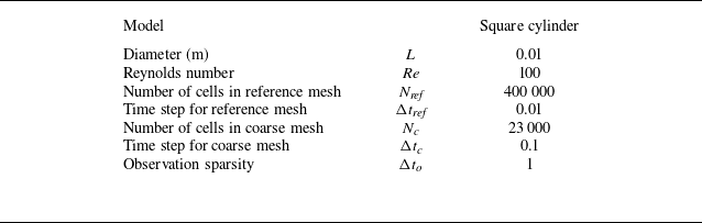


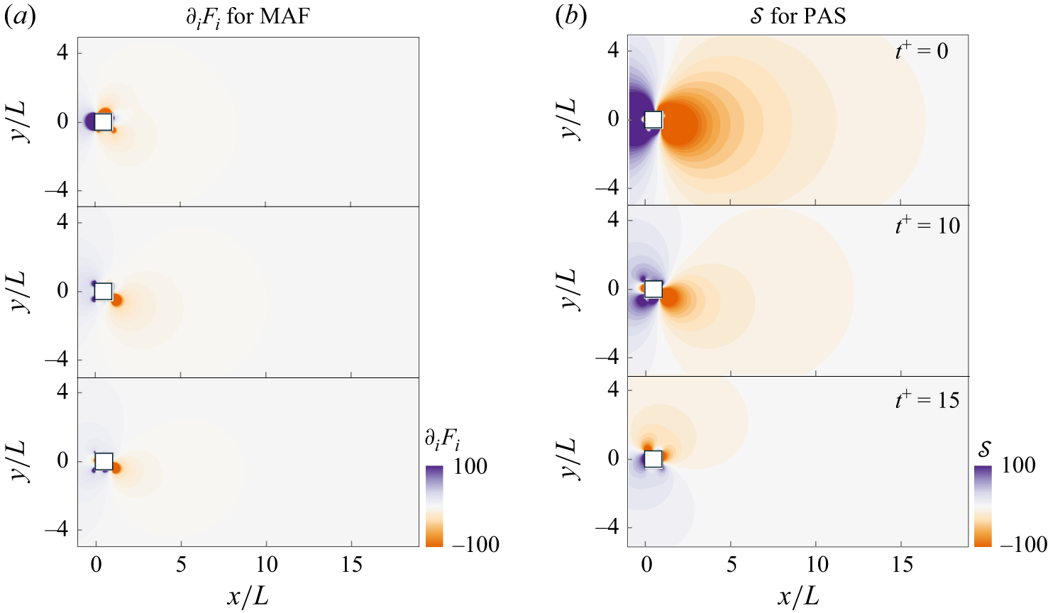
 ∂iFi
 S

 Q=104
 ξ
 η

 Ru′u′
 x/c=0.42
 Reτ=252
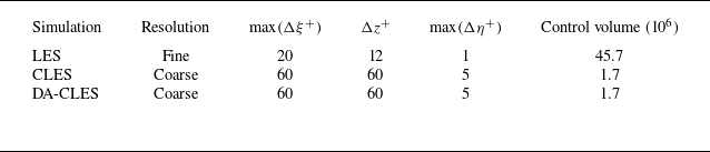
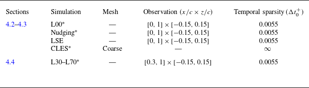
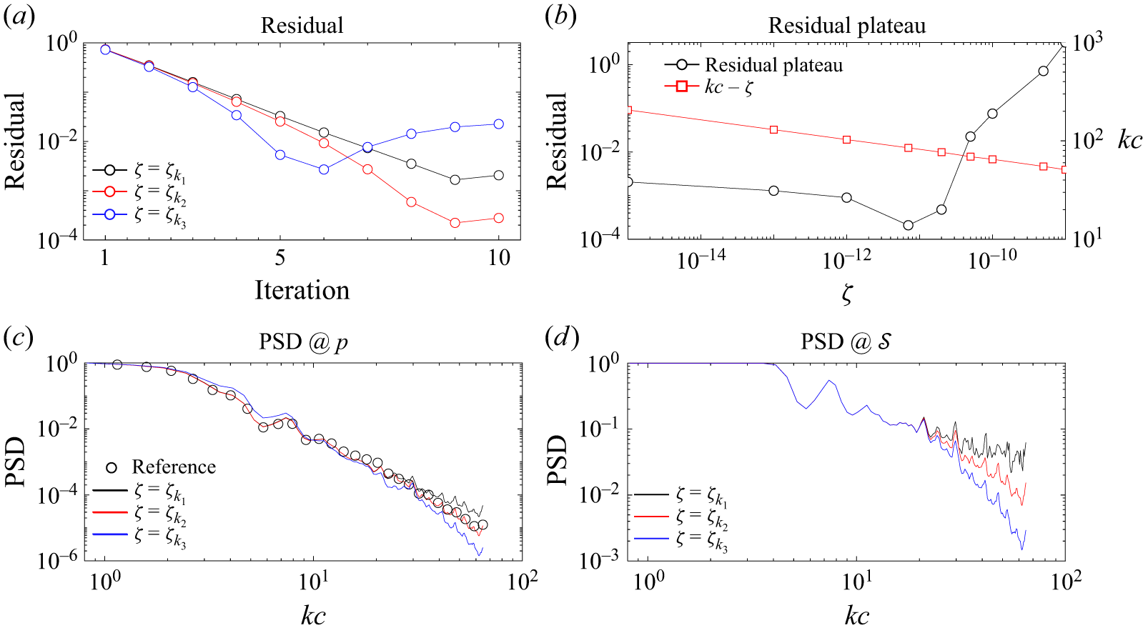
 ζ
 y+=5
 S
 y+=5

 S
 y+=5

 x−y
 z/c=0

 x−z
 y+=5

 x−y
 z/c=0

 x−z
 y+=5

 y+=5

 2.5


 z/c=0, y+=5
 y+=5

 St=7
 20


 St=7
 20

 z/c=0
 z/c=0


 y+=5
 t+=0.3
 0.65
 2.1

 log10(σ)
 f
 r
 St=20
 kzc=5π

 x/c=0.1
 y+=5
 St=7
 10
 20

 x/c=0.1
 y+=5
 St=7
 10
 20

 y+≈10
 PLES,max

 t+=8
 σ

 t+=8
 y+=10

 R2
 w'
 pw
 w'/U0
 y+=5
 z/c=0

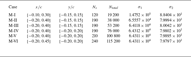
 σ1
 σ2
 kzc=0
 St=20
 Ns
 Ntotal


