





1. Introduction
Since the seminal works by the Chicago group (Deegan et al. Reference Deegan, Bakajin, Dupont, Huber, Nagel and Witten1997; Deegan et al. Reference Deegan, Bakajin, Dupont, Huber, Nagel and Witten2000), the coffee-ring effect (CRE) has garnered significant attention (Wilson & Ambrosio Reference Wilson and Ambrosio2023). In an evaporating sessile droplet, the pinning of the contact line imposes a radial outward flow to enforce mass conservation, transporting material from the centre toward the edge. In particle-laden droplets, this advective flow carries particles to the contact line, resulting in the characteristic ring-shaped deposit that has been extensively studied through simplified models of the CRE. However, in respiratory or complex-composition droplets, this transport involves not particles but solutes such as polymers, proteins or salts. The evaporation of such complex fluids is relevant in many situations of practical interest (see for example, Kajiya et al. Reference Kajiya, Kaneko and Doi2008; Mailleur et al. Reference Mailleur, Pirat, Pierre-Louis and Colombani2018; Basu & Mukherjee Reference Basu and Mukherjee2020; Guo et al. Reference Guo, Kinghorn, Zhang, Li, Dey Poonam, Tanner and Shum2021). Despite its relevance, the physics behind CRE formation in complex droplets remains less thoroughly explored.
In this work we focus on protein ring formation in sessile model respiratory droplets, even though similar problems arise in other complex fluids. Since the COVID-19 pandemic, this topic has gained significant attention in the disease transmission science community due to its implications for viral infectivity. Remarkably, viral particles (virions) can remain infectious for hours within the dry residue left by evaporated respiratory droplets (Morris et al. Reference Morris2021; Merhi et al. Reference Merhi, Atasi, Coetsier, Lalanne and Roger2022; Oswin et al. Reference Oswin2022). This is unexpected, as complete evaporation leads to high salt concentrations which creates, presumably, a harsh chemical environment for virions (Seyfert et al. Reference Seyfert, Rodríguez-Rodríguez, Lohse and Marin2022). One possible explanation for this paradox is that the droplet components – primarily salt and protein (Vejerano & Marr Reference Vejerano and Marr2018) – segregate during evaporation. A leading hypothesis, yet to be confirmed (Morris et al. Reference Morris2021; Martínez-Puig et al. Reference Martínez-Puig2025), is that virions are trapped in protein-rich regions, which protect them from salt-induced damage. Understanding how the protein ring forms is therefore needed to clarify how viral infectivity depends on relative humidity,
 $H_r$
.
Some recent studies have addressed this problem qualitatively from a biological perspective. For example, Kong et al. (Reference Kong, Sandhu, Qiu, Wu, Tian, Chi, Tao, Yang and Wang2022) and Pan et al. (Reference Pan, Duggal, Lakdawala, Rockey and Marr2025) analysed the final residue of evaporated sessile respiratory droplets and found that the final width of the protein ring depends on relative humidity – a behaviour that contrasts with predictions for particle-laden droplets. Another intriguing observation is a transition above
 $H_r = 80\,\%$
: at lower humidity, a protein-rich ring forms near the contact line, while at higher humidity protein is more uniformly distributed, without forming any distinctive structure. Despite these qualitative differences from the classical CRE in particle-laden systems, a dedicated theoretical framework for the ring formation in evaporating complex droplets – such as those containing both salt and protein – has not yet been developed.
A landmark mathematical analysis of the dynamics of deposition rings in particle-laden droplets was carried out by Popov (Reference Popov2005), whose framework has since been widely adopted. This model, developed specifically for particle suspensions, relies on two key assumptions. First, the evaporation rate is assumed to be decoupled from the solute transport problem, so it can be readily computed by solving the diffusion-driven vapour transport outside the drop for a constant vapour concentration at the air–droplet interface. Then, the evaporation rate thus obtained is used to compute the advective flux in the transport equation. Second, the formation of the deposition ring is driven by this advective flux, which transports particles toward the contact line. As the local particle concentration approaches the maximum packing fraction, further incoming particles cannot penetrate the already-deposited ring and instead accumulate at its inner edge, causing the ring to broaden towards the drop centre.
More sophisticated models, such as the one developed by Coombs et al. (Reference Coombs, Sprittles and Chubynsky2024b
) to study the so-called surface capture, build upon these principles. These hypotheses, reasonable for particle-laden suspensions, are crucial for solving the problem analytically as they enable the decoupling of the hydrodynamic and transport equations. A recent, very elegant, study by Moore et al. (Reference Moore, Vella and Oliver2021) introduced the effect of particle diffusion to investigate the early stages of the ring formation using asymptotic techniques. They solve an advection–diffusion equation for the particle concentration without imposing a maximum particle packing fraction. As a consequence, the particle concentration can grow unbounded, which leads to a progressive narrowing of the deposit, with the ring width decreasing in time and collapsing to a single line as
 $t\to t_{ev}$
. This behaviour is not consistent with experimental observations, which show a finite ring thickness at all times, including at the drying time. For this reason, most models aiming at quantitative comparison with experiments incorporate a maximum particle packing fraction.
We refer to these models as constant-activity models (CAM). Although they align well with experiments on particle-laden droplets – for instance, Coombs et al. (Reference Coombs, Chubynsky and Sprittles2024a
) successfully reproduced the measurements of Li et al. (Reference Li, Yang, Li and Song2016) – the concept of a particle packing fraction does not naturally extend to complex droplets. Moreover, these theories fail to capture several behaviours observed in polymeric or protein solutions. For example, studies have shown that in evaporating model respiratory droplets, the width of protein rings formed via the CRE depends on relative humidity (
 $H_r$
) (Kong et al. Reference Kong, Sandhu, Qiu, Wu, Tian, Chi, Tao, Yang and Wang2022; Pan et al. Reference Pan, Duggal, Lakdawala, Rockey and Marr2025). While this dependence may appear intuitive to experimentalists, it contradicts existing reduced models of the CRE. In Popov’s framework,
 $H_r$
only enters through the overall evaporation time scale, implying that the final deposition ring width should be independent of
 $H_r$
.
In contrast to particle-laden systems, where ring formation is commonly explained by the existence a maximum packing fraction, in polymeric or protein-rich droplets a more natural explanation involves water activity,
 $\chi _w$
. This thermodynamic property quantifies the water vapour pressure at an interface of an aqueous solution relative to that pure water, i.e.
 $C_{v\textit{ap}} = C_s\, \chi _w$
, where
 $C_{v\textit{ap}}$
is the concentration of water vapour at the air–droplet interface and
 $C_s$
is the water vapour saturation concentration in air. The water activity takes into account how solutes (like proteins or salts) reduce the evaporation rate. For solutes with a large affinity for water, such as some salts, the water activity can be much smaller than unity, which impacts strongly the evaporation dynamics. For an ideal mixture with solute mass fraction
 $w_p$
, the water activity is given by
 $\chi _w = 1 - w_p$
. For more complex solutions that depart from ideality, we still have, in general,
 $\chi _w \to 0$
as
 $w_p \to 1$
; that is, there is no water vapour at the interface of the droplet if there is no water inside the droplet at that location.
Roger et al. (Reference Roger, Liebi, Heimdal, Pham and Sparr2016) experimentally study the qualitative changes in evaporation behaviour in terms of water activity. Among their findings for an evaporating capillary is that, for a simple binary mixture, the evaporation rate becomes independent of ambient relative humidity for
 $H_r \leq 85\,\%$
. Salmon et al. (Reference Salmon, Doumenc and Guerrier2017) studied theoretically this surprising phenomenon. In their work on one-dimensional evaporation of supramolecular mixtures, they showed that evaporation can become nearly insensitive to ambient humidity. This occurs when the water activity drops sharply at high solute concentrations, so that the solute concentration at the drying interface becomes nearly independent of
 $H_r$
, leading to evaporation rates that vary only weakly with humidity. Huisman et al. (Reference Huisman, Digard, Poon and Titmuss2023) experimentally verified this theory by studying the evaporation of polyvinyl alcohol (PVA)–water solutions from open-ended capillaries. They observed that accumulation of PVA at the evaporating interface forms a polarisation layer, which affects both the local diffusivity and the water activity. As a result, the evaporation rate becomes nearly independent of ambient relative humidity for
 $H_r \leq 80\,\%$
.
Recently, Thayyil Raju et al. (Reference Thayyil Raju, Diddens, Rodríguez-Rodríguez, van der Linden, Zhang, Lohse and Sen2024) investigated the evaporation of glycerol–water solutions from open-ended capillary tubes using both experiments and theoretical modelling. By tracking the height of the upper meniscus, which is not exposed to evaporation, they identified an initial linear decrease in height over time – corresponding to the so-called constant-evaporation-rate stage. As evaporation progressed, glycerol concentration increased at the interface, modifying the water activity
 $\chi _{w}$
and triggering a transition to the falling-rate stage, where the meniscus velocity followed a power-law decay in time with an exponent of
 $-1/2$
, and a pre-factor that depends on the relative humidity and the initial glycerol concentration. For this same system, Milark et al. (Reference Milark, Salmon and Sobac2026) have explored the evaporation of a cylindrical drop confined in a Hele-Shaw cell. In this study, the spatio-temporal evolution of the water and glycerol concentrations is accurately measured using Mach–Zehnder interferometry. The measurements of both concentration fields and drying kinetics led the authors to the determination of both the mutual diffusion coefficient and water activity, proving the ability of this kind of model to describe evaporation in confined systems once the water activity and the correct value of the diffusion coefficient are incorporated into the formulation.
A number of studies have also focused on the role of water activity in the evaporation and stability of respiratory droplets. For example, Merhi et al. (Reference Merhi, Atasi, Coetsier, Lalanne and Roger2022) combined experimental measurements with theoretical modelling to highlight that incorporating a non-ideal thermodynamic water activity establishes an equilibrium droplet size that becomes independent of relative humidity. Seyfert et al. (Reference Seyfert, Rodríguez-Rodríguez, Lohse and Marin2022) investigated the evaporation of model respiratory droplets on superhydrophobic substrates. They found that, at high relative humidity, evaporation halts once the water activity of the solution equals the ambient humidity, i.e.
 $\chi _{w}(w_s) = H_r$
. Notably, this condition is reached before salt efflorescence occurs (at 20
 $\,^\circ$
C for
 $H_r \geq 0.75$
), resulting in droplets that remain stable and liquid indefinitely without fully drying. More recently, Haut et al. (Reference Haut, Atasi and Sobac2025) studied theoretically how the effects of a non-constant water activity impact both the sedimentation and drying times of expelled spherical respiratory droplets. Their findings are in agreement with the experimental results of Merhi et al. (Reference Merhi, Atasi, Coetsier, Lalanne and Roger2022), which show that the equilibrium droplet radius is independent of relative humidity for values below approximately 70 %.
These examples illustrate a broader class of systems where evaporation rates are strongly influenced by the composition at the evaporating interface. This effect must be incorporated into any theoretical framework aiming to describe the CRE in complex droplets. As we will demonstrate for the case of model respiratory droplets, including the dependence of the water activity coefficient,
 $\chi _w$
, on the protein mass fraction,
 $w_p$
, allows us to explain key experimental observations, such as the relative humidity dependence of the time evolution and final value of the ring width.
Our objective is to integrate recent advances from these studies into a comprehensive understanding of coffee-ring formation in complex droplets, with a particular focus on model respiratory droplets as a case study. To this end, § 2 presents experimental observations of protein ring formation using fluorescence microscopy. In § 3, we derive a minimal model that captures the key mechanisms driving the CRE in these complex solutions. Section 4 details the formation mechanism of the protein ring, discusses the roles of salt and protein-dependent diffusivity, compares the theoretical prediction with our experimental results and presents some limitations of the model. Finally, the manuscript concludes with a summary and outlook in § 5.
2. Experiments
We evaporate artificial saliva droplets following the composition used by Vejerano & Marr (Reference Vejerano and Marr2018), namely milliQ water with
 ${9}\,\textrm {g l}^{-1}$
of NaCl (Sigma-Aldrich),
 ${3}\,\textrm {g l}^{-1}$
of porcine gastric mucin type III (Sigma-Aldrich) and
 ${0.5} \,\textrm {g l}^{-1}$
of the pulmonary surfactant 1,2-dihex-adecanoyl-sn-glycero-3-phosphocholine. Mucin, the main protein found in respiratory fluids, will be particularly important here, as it is the solute responsible for the ring formation. This composition is commonly used in experimental studies investigating the decay rates of viral infectivity (Pan et al. Reference Pan, Duggal, Lakdawala, Rockey and Marr2025).
2.1. Experimental set-up
We deposit sessile model respiratory droplets of initial volume
 $V_0=0.3\pm 0.1 \,{\unicode{x03BC}} \textrm {l}$
on
 $\mu$
-Dish 35 mm, high glass-bottom dishes (Ibidi). These microPetri dishes enable high-resolution imaging and do not exhibit autofluorescence. The evaporation follows a constant-radius mode, which is consistent across all experiments and throughout the droplet lifetime. This behaviour results from the accumulation of mucin at the substrate, which pins the contact line. The droplets are evaporated inside a humidity-controlled chamber, at a constant relative humidity (
 $H_r$
) which varied between
 $30\,\%$
and
 $70\,\%$
among different experiments. We use the temperature and humidity sensor DHT11 with an accuracy
 $\pm 5 \,\%$
in relative humidity and
 $\pm 1\,^\circ$
C in temperature. The room temperature varies among experiments between
 $20\,^\circ$
C and
 $28\,^\circ$
C. To increase humidity, we introduce humid air into the chamber by recirculating it through a water bottle. To desiccate the air, we recirculate it through a separate bottle containing calcium phosphate, a highly hygroscopic salt. This configuration is adapted from Boulogne (Reference Boulogne2019) in order to fit in the reduced space available on a microscope. An schematic of our experimental set-up is shown in figure 1.
Schematic of the procedure used to obtain the radial intensity profile. (a) Time-lapse images of the evaporating droplet are acquired using an epifluorescence microscope inside a chamber controlled by a temperature and humidity sensor (T & RH sensor). (b) Example of a fluorescence image obtained during evaporation. (c) The droplet is segmented into concentric annular regions, and the mean fluorescence intensity is computed for each region. For visualisation purposes, fewer regions are shown than were used in the actual analysis. (d) From this process, the radial intensity profile is extracted for each image.

Figure 1. Long description
Panel A: A diagram shows the setup for capturing time-lapse images of an evaporating droplet using an epifluorescence microscope inside a humidity-controlled chamber. The setup includes a controlled chamber with a temperature and relative humidity sensor, a respiratory-like droplet, and a 10x objective lens. An LED light source and a camera are used to capture the images. Panel B: A fluorescence image obtained during the evaporation process highlights a protein rim at the edge of the droplet. The scale bar indicates 250 micrometers. Panel C: The droplet is segmented into concentric annular regions, and the mean fluorescence intensity is computed for each region. The image shows fewer regions for visualization purposes. Panel D: A graph displays the radial intensity profile extracted from the fluorescence images. The x-axis represents the radial distance in micrometers, and the y-axis represents the intensity in arbitrary units. The graph shows a peak in intensity at the edge of the droplet, indicating the protein rim.
To evaluate the spatial distribution of proteins, we utilised the enhanced autofluorescence of mucin, a highly glycosylated protein abundant in model respiratory droplets. Mucin exhibits high autofluorescence compared with other proteins due to its extensive glycosylation, which can generate fluorescent compounds through sugar oxidation or glycation. The evaporation dynamics was monitored using an inverted widefield fluorescence microscope (Leica DMi8) equipped with a CoolLED pE-4000 illumination system and an Orca-Flash 4.0 sCMOS camera (Hamamatsu). Images were acquired using a 10
 $\times$
/0.32 HC PL FLUO objective. Excitation was performed using a 405 nm LED. The microscope was equipped with a quad-band fluorescence filter set (QUA-T), however, only the channel corresponding to excitation at 405 nm and emission collection at 420–480 nm was used in this study. This wavelength is the closest to the ultraviolet (UV) range, where optimal excitation for proteins occurs, that we have available in our microscope. Despite not being able to excite the protein fluorescence emission at its optimal wavelength, still enough autofluorescent signal is emitted when illuminating in the UV-blue range and imaging the emission in the blue band Lakowicz (Reference Lakowicz2006). The exposure time was set to 20 ms per acquisition. To prevent excessive heating of the droplet, we capture images every 5 s and verify that the evaporation time matches the theoretical predictions described by Seyfert et al. (Reference Seyfert, Rodríguez-Rodríguez, Lohse and Marin2022).
Due to the axisymmetric nature of the protein rim formation, we focus on the radial intensity profile, defined as
 \begin{align} I(r) = \frac {1}{2\pi } \int _0^{2\pi } i(r,\varphi )\, {\rm d}\varphi , \end{align}
where
 $i(r,\varphi )$
is the local intensity in polar coordinates. As the droplet’s contact line is not a perfect circle, the radial intensity
 $I(r)$
is estimated through the following procedure. First, the contact line is extracted from the image and represented as a spline. The centroid is then calculated using
 $A = ({1}/{2}) \sum _{i=1}^{n} (x_i y_{i+1} - x_{i+1} y_i)$
,
 $x_c =( {1}/{6A}) \sum _{i=1}^{n} (x_i + x_{i+1})(x_i y_{i+1} - x_{i+1} y_i)$
and
 $y_c =({1}/{6A}) \sum _{i=1}^{n} (y_i + y_{i+1})(x_i y_{i+1} - x_{i+1} y_i)$
, where
 $(x_c, y_c)$
is the centroid of the spline defined by the ordered vertices
 $(x_i, y_i)$
. The droplet is then divided into annular regions by constructing inward homothetic splines of the contact line (figure 1
c). Within each of these regions, the local intensity is integrated to obtain the corresponding radial intensity. Each homothetic spline is assigned a radius, defined as the mean distance of its points to the centroid of the original contact line. The radial position associated with each annular region is taken as the average of the radii of its inner and outer bounding splines.
In order to obtain the height-averaged mass fraction of mucin,
 $\overline {w}_p$
, from the radial intensity,
 $I(r)$
, we follow a similar approach to that employed by Kajiya et al. (Reference Kajiya, Kaneko and Doi2008). We assume that the fluorescence intensity follows the relationship
 \begin{align} I(r) = K \overline {w}_p(r) h(r), \end{align}
where
 $K$
is a proportionality constant, and
 $h(r)$
is the height of the drop. To verify the linear relationship between fluorescence intensity, height-integrated protein mass fraction and droplet height, we performed a series of calibration experiments. A calibration chamber was constructed using glass slides arranged in an L-shaped geometry, where
 $L$
denotes the horizontal length of the base and
 $H$
the vertical height. A thin coverslip was placed on top to enclose the chamber. This configuration creates a wedge-shaped volume of solution with a linearly varying height
 $h = x (H/L)$
, where
 $x$
is the horizontal direction. By translating the microscope objective along this direction, we could access fluorescence signals at known and controllable sample heights, enabling calibration of the fluorescence response as a function of height. We acquired fluorescence images of protein solutions with
 $\overline {w}_p = 0.003,\, 0.025,\, 0.05,\, 0.1$
. Higher protein mass fraction (
 $\overline {w}_p \gt 0.1$
) could not be dissolved in water and salt to produce a uniform mixture. For each protein mass fraction, we verified the linear relationship between fluorescence intensity and solution height (see figure 2
a). To test the dependence on
 $\overline {w}_p$
, we found that the slopes of the fitted lines relating intensity to height scale linearly with the height-integrated protein mass fraction (see figure 2
b). As a consequence of this linearity, from (2.2), the total amount of light intensity
 $\mathcal{I}(t)$
follows
 \begin{align} \mathcal{I}(t)=\int _0^{R_c}2\pi r I(r,t){\rm d}r=\int _0^{R_c}2\pi r K \overline {w}_p(r,t) h(r,t){\rm d}r= K M_p, \end{align}
where
 $R_c$
is the contact radius and
 $M_p$
is the total amount of protein in the droplet, that remains constant throughout the experiment. At the beginning of the evaporation process, the relatively high contact angle (approximately
 $60^\circ$
) leads to optical reflections near the contact line, which artificially increase the measured fluorescence intensity
 $\mathcal{I}(t)$
. To avoid this artefact, our analysis begins only after these reflections disappear and the system enters a regime in which
 $\mathcal{I}(t)$
remains constant. Within this regime, the intensity varies by less than 1 % throughout each experiment. Following this stable period, droplets exposed to low and medium relative humidity eventually crystallise, causing a sharp increase in
 $\mathcal{I}(t)$
. Our analysis is therefore restricted to the temporal window between the disappearance of initial reflections and the onset of crystallisation (see figure 2
c).
Calibration of fluorescence intensity as a function of droplet height and protein mass fraction. (a) Fluorescence intensity profiles at different relative heights
 $h^*$
for varying protein mass fraction
 $C_p = 0.003, 0.025, 0.1$
, confirming the linear relationship between intensity and height. (b) Slopes of the fitted lines,
 $m$
, from (a) demonstrating the linear dependence of fluorescence intensity on protein mass fraction. (c) Representative time evolution of the total fluorescence intensity, showing distinct regimes during evaporation. All quantitative analyses presented throughout this article are based on data from the constant-intensity regime.

It should be noted that although both mucin and salt crystals were visualised using fluorescence microscopy with excitation at 405 nm and emission detection between 420–480 nm, only mucin exhibits intrinsic autofluorescence in this spectral window. Inorganic salt crystals do not emit fluorescence under these conditions. The signal observed from salt crystals is therefore attributed primarily to light scattering rather than true fluorescence emission. Additionally, it is possible that mucin molecules become adsorbed or deposited onto the surfaces of salt crystals during droplet evaporation, resulting in localised fluorescence signals that spatially coincide with the crystal structures. A detailed investigation of this complex interplay is beyond the scope of the present work, but it constitutes an interesting avenue for future research.
From fluorescence experiments, we obtain the radial intensity as
 $ I(r) = K \, \overline {w}_p \, h$
. However, due to spatial constraints within the microscope set-up, it is not possible to image the droplet from the side during fluorescence experiments. As a result, we cannot directly measure the interface height profile
 $ h(r,t)$
. To circumvent this limitation, we work with the height-integrated protein fraction
 $\phi _p = h\,\overline {w}_p$
when analysing the spatial distribution of protein.
2.2. Experimental results
Fluorescence images showing (a) the initial homogeneous distribution of protein, (b) the formation of a peripheral protein ring and (c) final crystallisation. Droplet evaporated at
 $H_r=30.4\,\%$
and
 $T=20.5\,^\circ$
C.

As evaporation progresses, protein begins to accumulate near the contact line, forming a protein ring. We observe that this protein ring increases in both intensity and width over time (see figure 3). Notably, in model respiratory droplets, a relevant feature of the protein ring is its width,
 $\delta$
, which has been linked to the low decay rates of virions’ infectivity in dry residues of model respiratory droplets (Huang et al. Reference Huang, Wang and Vikesland2021). Protein is expected to shroud virions, slowing their loss of infectivity (Wardzala et al. Reference Wardzala, Wood, Belnap and Kramer2022). This suggests that a wider protein-rich region could help virions to remain infective for a longer period.
We define the width of the coffee ring,
 $\delta$
, as that of the peak at half prominence (figure 1
d). We adopt this definition because measuring the peak width at half height, as done in analytical theories like those of Popov (Reference Popov2005) and Moore et al. (Reference Moore, Vella and Oliver2021), is experimentally challenging for high relative humidity. In these cases, the height of the peak does not allow for easy identification of the intersection at half-height in the inner part of the protein ring.
The most striking phenomena we found in experiments are that the width
 $\delta$
follows a different dynamics for different relative humidities (see figure 4
a and Appendix A) and that the maximum height-integrated protein fraction
 $\phi _p$
of the protein ring decreases as the relative humidity increases (see figure 4
c and Appendix A). As explained on the introduction, in CAM, the width of the coffee ring has been found to follow the same scaling law across all values of the relative humidity. However, as shown in figure 4(a), this behaviour does not hold for protein ring formation in sessile model respiratory droplets. In this figure we show the time evolution of the rim width for drops evaporating at different humidity, with the time scaled with the diffusive time scale,
 $t_d = \rho R_c^2 / D_{v\textit{ap}} C_{{s}}(1-H_r)$
. This time scale is computed with the density of water,
 $\rho$
, the contact radius,
 $R_c$
, the diffusivity of water vapour in air,
 $D_{v\textit{ap}}$
, the saturation concentration of water vapour in air,
 $ C_{{s}}$
, and the ambient relative humidity,
 $H_r$
. Because of experimental limitations in determining the exact onset of deposition, the initial time of each experiment carries some uncertainty. To account for this, we reset the origin of the temporal axis by introducing
 $t_{10\,\%}$
, defined as the time at which the protein mass accumulated in the ring reaches
 $10\,\%$
of the total protein mass in the droplet.
Experimental results. (a) Temporal evolution of the ring width,
 $\delta$
. (b) Mass of protein,
 $m_p$
, in the ring normalised by the total protein mass in the droplet,
 $M_p$
, as a function of time. (c) Dependence of the maximum height-integrated protein fraction, normalised by the total protein mass in the droplet divided by the contact area
 $A_c$
, with the relative humidity.

Figure 4. Long description
Panel A: A line graph shows the temporal evolution of the ring width, normalized by the droplet radius, as a function of normalized time. The x-axis represents normalized time, and the y-axis represents the normalized ring width. The graph includes multiple lines in varying shades of blue and green, with an inset showing the ring width over time in micrometers. Panel B: Another line graph displays the mass of protein in the ring, normalized by the total protein mass in the droplet, as a function of normalized time. The x-axis represents normalized time, and the y-axis represents the normalized protein mass. The graph includes multiple lines in varying shades of blue and green, with an asterisk marking crystallization points. Panel C: A scatter plot illustrates the dependence of the maximum height-integrated protein fraction, normalized by the total protein mass in the droplet divided by the contact area, on relative humidity. The x-axis represents relative humidity, and the y-axis represents the normalized protein fraction. The plot includes multiple data points in green.
Figure 4(a) shows that the evolution of the rim width
 $\delta$
depends on the relative humidity
 $H_r$
in two distinct ways. First, the final rim width attained prior to crystallisation varies with
 $H_r$
, with larger values observed at higher relative humidity; this dependence is absent from the model of Popov (Reference Popov2005), in which all curves collapse when time is rescaled by the diffusive time scale
 $t_d$
. Second, the growth rate of the rim width differs between humidities: when time is non-dimensionalised by
 $t_d$
,
 $\delta$
grows more slowly at low and intermediate
 $H_r$
than at high
 $H_r$
. The slopes are different over the evolution, and at high relative humidity
 $\delta$
saturates at late times. In more sophisticated theories, such as those of Coombs et al. (Reference Coombs, Sprittles and Chubynsky2024b
) and Moore et al. (Reference Moore, Vella and Oliver2021), the temporal evolution of the ring width exhibits a Péclet-dependent offset while retaining a universal slope. In contrast, our experiments reveal an increase of the slope with increasing
 $H_r$
, a feature not captured by existing coffee-ring models. This behaviour can be rationalised by accounting for the dependence of water activity on both salt and protein mass fractions (see § 4 for a detailed discussion).
3. Mathematical model
In this section, we present a minimal theoretical model aimed at capturing the essential dynamics of the CRE in complex droplets, as observed in our experiments (see § 2). The goal is not to achieve a one-to-one quantitative comparison with the experimental results, but rather to use the experimental observations as motivation to explore physical mechanisms that are not adequately explained by existing theoretical models.
As discussed in the Introduction, most existing models of the CRE have been developed in the context of particle-laden droplets. To reproduce the formation of a realistic ring width, these models typically rely on the assumption of a maximum packing fraction
 $w_{p_c}$
(Popov Reference Popov2005; Kaplan & Mahadevan Reference Kaplan and Mahadevan2015; Coombs et al. Reference Coombs, Sprittles and Chubynsky2024b
). This assumption leads to a separation of the droplet into two distinct regions: one where the local particle concentration is exactly
 $w_{p_c}$
, forming the dense particle ring, and another where the concentration remains below
 $w_{p_c}$
, corresponding to a dilute region. These frameworks allow for a decoupling of the hydrodynamics from the transport problem, simplifying the analysis to make it tractable analytically. While this approach is appropriate for particle suspensions, it becomes less adequate when applied to polymeric or protein solutions as, in such systems, there is no natural extension of a maximum packing fraction. As a result, the use of
 $w_{p_c}$
in this context is somewhat arbitrary in these systems and does not accurately capture the underlying physics of polymer or protein ring formation. A more sophisticated approach, adopted by Coombs et al. (Reference Coombs, Chubynsky and Sprittles2024a
), is to introduce a concentration-dependent viscosity, which effectively models the ring as a region where particles progressively jam until they reach a critical concentration. An advantage of this approach is that it is equally valid for particle suspensions and for solutions of polymers or other complex molecules. In such a case, the critical concentration can be, for instance, that at which a gel transition occurs. However, as we will discuss below, this approach is still not able to explain the effect that the ambient relative humidity is observed to have on the drop dry deposit, as evaporation is still decoupled from the transport dynamics.
In contrast, here, we adopt a different approach in which the entire droplet is treated as a single continuous phase. Consequently, the equations we derive are valid throughout the entire droplet and remain applicable at all times during the evaporation process.
As has been shown (Martínez-Puig et al. Reference Martínez-Puig2025), the flow pattern in respiratory droplets can be recirculatory due to natural convection. In other contexts, recirculation may also arise from Marangoni stresses (Marín et al. Reference Marin, Karpitschka, Noguera-Marín, Cabrerizo-Vílchez, Rossi, Kähler and Rodríguez Valverde2019; Dekker et al. Reference Dekker, Rocha, Diddens and Lohse2025). For a detailed two-dimensional model that accounts for these phenomena, we refer the interested reader to Diddens et al. (Reference Diddens, Li and Lohse2021), Dekker et al. (Reference Dekker, Rocha, Diddens and Lohse2025) and Martínez-Puig et al. (Reference Martínez-Puig2025). In the present work, however, our goal is to develop a minimal model that explains the mechanism behind the coffee-ring effect in complex droplets. To that end, we adopt the lubrication approximation and derive a one-dimensional model to describe the hydrodynamics and solute transport within the droplet.
3.1. Flow problem
In order to apply the lubrication approximation, we assume that
 $\epsilon = h_0 / R_c \ll 1$
, where
 $h_0$
is the initial height of the droplet at
 $r = 0$
. Also, we neglect the effect of gravity. This has two implications: first, we assume a small Bond number
 $\mathrm{Bo} = \rho g R_c^2 / \gamma ^* \ll 1$
, where
 $\gamma ^*$
is the surface tension. This hypothesis implies that the shape of the drop’s surface is not affected by gravity, and is valid for aqueous droplets with radii smaller than a millimetre. Second, we also neglect buoyancy forces in the hydrodynamic and transport equations. In point of fact, the stratification caused by evaporation can drive a recirculatory buoyancy-driven flow in our system at short times, when the drop is not shallow. This is due to the fact that the ratio between the buoyancy-driven and the capillary flows scales as
 $\varepsilon ^5{Ra}$
, where
 $ \textit{Ra} = \partial _w\rho g R_c^3 / \mu ^* D^*_p$
is a Rayleigh number (Diddens et al. Reference Diddens, Li and Lohse2021). In this definition,
 $\partial _w\rho$
is the derivative of the solution’s density with the solute mass fraction,
 $\mu ^*$
the liquid viscosity and
 $D^*_p$
the diffusivity of the solute. For the droplet sizes and compositions of our experiments,
 $ \textit{Ra} \sim 10^6$
, which generates a recirculatory flow driven by density stratification at short times when
 $\varepsilon$
is still not small enough (Martínez-Puig et al. Reference Martínez-Puig2025) (see also Appendix F). Nonetheless, we neglect these effects in what follows for two reasons: first, we work with the height-averaged radial velocity
 $\bar {u}_r$
and protein mass fraction
 $\bar {w}_p$
, thus the velocity and concentration profiles do not appear explicitly in our formulation. Second, the buoyancy-driven recirculatory flow does not transport any net mass along the radial direction, for the reasons pointed out by Diddens et al. (Reference Diddens, Li and Lohse2021), so its effect on the solute transport can be neglected in a first approximation.
Marangoni effects can also be incorporated within the lubrication framework. However, previous studies (Du et al. Reference Du, Zhang and Shen2022; Martínez-Puig et al. Reference Martínez-Puig2025) have shown that surface tension gradients are negligible in protein-laden mixtures, due to the accumulation and jamming of proteins at the interface. Thus, we neglect surface tension variations on the model. We further assume that the flow is axisymmetric so we have, in cylindrical coordinates,
 \begin{align} \frac {\partial h^*}{\partial t^*}+\frac {1}{r^*} \frac {\partial }{\partial r^*}\left (r^* h^* \bar {u}_r^*\right )=-\frac {J^*}{\rho ^*}, \quad \bar {u}_r^*=-\frac {h^{* 2}}{3 \mu ^*} \frac {\partial p^*}{\partial r^*}, \quad p^*=p_{a t m}^*-\frac {\gamma ^*}{r^*} \frac {\partial }{\partial r^*}\left (r^* \frac {\partial h^*}{\partial r^*}\right )\!, \end{align}
where
 $h$
is the height of the droplet,
 $t$
is the time,
 $r$
is the radial coordinate,
 $J$
is the local evaporation rate,
 $\rho$
is the density of the suspension,
 $\bar {u}_r$
is the height-averaged radial velocity,
 $\mu$
is the suspension viscosity,
 $p$
is the pressure,
 $p_{\textit{atm}}$
is the atmospheric pressure and
 $\gamma$
is the surface tension of the suspension. The superscript
 $^*$
denotes dimensional variables. Equation (3.1) is subject to symmetry boundary conditions at the symmetry axis
 \begin{align} \frac {\partial h^*}{\partial r^*}=Q^* = 0 \quad \mathrm{at}\quad r^*=0, \end{align}
where
 $Q^* = r^* h^* \bar {u}_r^*$
is the local flow rate. At the contact line there is no flux and the height is zero
 \begin{align} h^*=Q^* = 0 \quad \mathrm{at}\quad r^*=R_c. \end{align}
As we have neglected the influence of gravity on the droplet shape the initial condition is that of a paraboloid of revolution (equivalently to a spherical cap in the lubrication approximation)
 \begin{align} h^*= \frac {h_0}{R_c^2} \big(R_c^2-r^*{^2} \big) \quad \mathrm{at}\quad t^*=0. \end{align}
3.2. Solute transport problem
We derive a transport equation for the height-averaged solute mass fraction
 $\bar {w}_p$
integrating vertically from
 $z^* = 0$
to
 $z^* = h^*(r^*, t)$
the two-dimensional, axisymmetric transport equation. Doing so, we obtain
 \begin{align} \frac {\partial }{\partial t^*}\left (h^* \overline {w}_p\right )+\frac {1}{r^*} \frac {\partial }{\partial r^*}\left (r^* h^* \bar {u}_r^* \overline {w}_p\right )=\frac {1}{r^*} \frac {\partial }{\partial r^*}\left (D_p^* r^* h^* \frac {\partial \overline {w}_p}{\partial r^*}\right )\!. \end{align}
This equation is subjected to symmetry conditions at the axis
 $r=0$
 \begin{align} \frac {\partial \overline {w}_p}{\partial r^*} = 0 \quad \mathrm{at}\quad r^*=0. \end{align}
Moreover, as the solute is non-volatile, we impose a no-flux condition at the contact line
 \begin{align} r^* h^* \bar {u}_r^* \overline {w}_p-D_p^* r^* h^* \frac {\partial \overline {w}_p}{\partial r^*}=0 \quad \mathrm{at}\quad r^*=R_c. \end{align}
We further assume that the solute is initially well mixed so the initial condition is
 \begin{align} \overline {w}_p = w_{p_0} \quad \mathrm{at}\quad t^*=0, \end{align}
where
 $w_{p_0}$
is the initial protein mass fraction.
To remain consistent with the equations derived in the previous subsection, we also adopt here the lubrication approximation,
 $\epsilon \ll 1$
. Also, we regard the solute as well mixed along the
 $z$
direction. This amounts to substitute
 $\overline {u_r^* w_p}$
by
 $\bar {u}_r^*\bar {w}_p$
in (3.5) and (3.7). The solute can be considered well mixed if a vertical Péclet number is small, so diffusion is able to smear the stratification caused by the relative motion between the liquid and the receding interface. As explained in Ramírez-Soto & Karpitschka (Reference Ramírez-Soto and Karpitschka2022), the vertical Péclet number is of the order
 $ \textit{Pe}_z \sim \epsilon ^2 \textit{Pe} = \epsilon ^2 \bar {u}^*_r R_c / D^*_p$
. In this expression, one factor
 $\epsilon$
arises from projecting the radial velocity onto the direction perpendicular to the interface and the other from the fact that diffusion occurs mainly along that same direction.
As will be shown in § 4, we get values of order
 $ \textit{Pe} \sim {\mathcal O}(10)$
in our experiments. Consequently, the vertical Péclet number is larger than unity until
 $\epsilon$
does not decrease below
 $\epsilon \approx 0.3$
. This occurs for a contact angle of approximately
 $\theta \approx 30^\circ$
. Thus, at short times, the solute could not be regarded at well mixed. However, we must take into account that the transport dynamics at the rim is local (Moore et al. Reference Moore, Vella and Oliver2021), since mass accumulates preferentially near the contact line. So, since the drop height is small in the rim region, the local value of
 $ \textit{Pe}_z$
is in fact smaller there than the global value. Moreover, a substantial part of the rim mass accumulates at times close to full evaporation, when
 $\epsilon \ll 1$
. All in all, the vertical Péclet number relevant to describe the solute transport towards the rim can be deemed as small, although it is not during the first part of the evaporation process and outside the rim region.
3.3. Evaporation rate
Up to this point, if viscosity and diffusivity are assumed to be constant and independent of solute concentration, the hydrodynamic problem is decoupled from the transport of solute. However, this decoupling breaks down when we account for the fact that evaporation itself depends on local solute concentration. It is well established that the water activity – and therefore the local evaporation rate – is a function of solute concentration for many polymers and proteins. This introduces a critical feedback mechanism: the solute concentration affects the evaporation rate (Salmon et al. Reference Salmon, Doumenc and Guerrier2017; Thayyil Raju et al. Reference Thayyil Raju, Diddens, Rodríguez-Rodríguez, van der Linden, Zhang, Lohse and Sen2024), which in turn modifies the flow field and solute transport. In the following we describe how to account for this coupling through the evaporation rate.
The large evaporation time scale,
 $ t_{{ev}} \sim 10^2 \, \mathrm{s}$
, compared with the characteristic diffusive time scale of water vapour in the gas phase,
 $ t_{d_G} = R_c^2 / D_{v\textit{ap}} \sim 10^{-1} \, \mathrm{s}$
, justifies the assumption of quasi-steady diffusion of water vapour in the surrounding air
 \begin{align} {{\nabla} ^2}^\ast C_{vap}^\ast =0. \end{align}
Provided that the droplet is thin, the Dirichlet condition at the droplet–air interface is imposed at
 $z^*=0$
 \begin{align} C_{vap}^\ast = C_s \chi _w \quad \mathrm{at}\quad z^*=0, \ 0\lt r^*\lt R_c. \end{align}
This condition arises from the assumption of thermodynamic equilibrium between the droplet and the surrounding vapour phase. The water activity,
 $\chi _w$
, accounts for the reduction in the equilibrium vapour concentration at the droplet interface, due to the presence of solutes, relative to that of a pure water droplet. This condition needs to be complemented with the symmetry condition
 \begin{align} \frac {\partial C_{vap}^*}{\partial r^*}=0 \quad \mathrm{at}\quad r^*=0, \end{align}
the no-flux condition on the substrate outside the droplet
 \begin{align} \frac {\partial C_{vap}^*}{\partial z^*}=0 \quad \mathrm{at}\quad r^*\gt R_c, \end{align}
and the far-field condition
 \begin{align} C_{vap}^*=C_s H_r \quad \mathrm{at}\quad r^*\to \infty , \ z^*\to \infty . \end{align}
Formally, on a thin droplet where the water vapour transport is diffusive, the evaporation rate is
 \begin{align} J^*=-D_{vap}^*\frac {\partial C_{vap}^*}{\partial z^*} \quad \mathrm{at}\quad z^*=0, \ 0\lt r^*\lt R_c. \end{align}
This problem can be solved analytically, as shown by Popov (Reference Popov2005), for the case of a constant Dirichlet boundary condition at the air–water interface, i.e. when the water activity
 $\chi _w$
remains constant. However, to capture the rich phenomenology of the evaporation dynamics of polymeric or protein solutions, the water activity must be treated as concentration-dependent,
 $\chi _w(\overline {w}_p)$
, and therefore it varies along the droplet radius. This class of problem is classical in potential theory (Copson Reference Copson1947). One approach is to apply the Hankel transform, which reduces the problem to a dual integral equation (Noble Reference Noble1958), although this method is algebraically cumbersome. A more elegant and tractable solution, based on techniques from complex analysis, was presented by Green & Zerna (Reference Green and Zerna1992), yielding the following expression for the evaporation rate:
 \begin{align} J^*=-D_{vap}C_s\frac {1}{r^*} \frac {\partial }{\partial r^*} \int _{r^*}^{R_c} \frac {r' g(r') \, \mathrm{d} r'}{\sqrt {r^2-r'^2}} , \end{align}
where
 \begin{align} g(r')=\frac {2}{\pi } \frac {{d}}{\mathrm{d} r'} \int _0^{r'} \frac {r \left (\, \chi _w(r)-H_r\right ) \, \mathrm{d}r}{\sqrt {r'^2-r^2}}. \end{align}
Notably, this formulation recovers the analytical solution of Popov (Reference Popov2005) as a special case when
 $\chi _w$
is constant. Solving these integrals analytically for a non-constant
 $\chi _w$
remains far from trivial. Fu et al. (Reference Fu, Cao and Cao2005) derived an explicit expression for the auxiliary function
 $g(r')$
under the assumption that
 $\chi _w(r)$
can be represented as a polynomial. This allows a symbolic computation of the evaporation rate
 $J^*$
using mathematical software. However, when strong spatial gradients in
 $\chi _w$
are present, polynomial approximations tend to introduce spurious oscillations in the evaporation rate. To overcome this limitation, we adopt a semi-analytical approach that is robust regardless of the smoothness of
 $\chi _w$
. Specifically, we represent
 $\chi _w$
using cubic splines, which permits an analytical solution for
 $g(r')$
, followed by a numerical integration to evaluate
 $J^*$
. The strength of this method lies in the ability of cubic splines to approximate arbitrary continuous functions without inducing artificial oscillations. Technical details of the spline-based implementation are provided in Appendix D.
3.4. Non-dimensionalisation
The characteristic scales of the problem are those induced by evaporation. Thus the characteristic velocity is given by evaporation as
 $v_c=J_c^*/\rho ^*\epsilon$
, where
 $J_c^* =D_{vap} C_s(1-H_r)/R_c$
. Based on this scale, we introduce the following dimensionless variables:
 \begin{align} \begin{array}{c} r = \dfrac {r^*}{R_c^*}, \quad z = \dfrac {z^*}{\epsilon R_c^*}, \quad \bar {u}_r = \dfrac {\epsilon \rho ^* \bar {u}_r^*}{J_c^*}, \quad t = \dfrac {J_c^* t^*}{\epsilon \rho ^* R^*}, \\[12pt]h = \dfrac {h^*}{\epsilon R^*}, \quad p = \dfrac {(p^* - p_{{atm}}^*) \rho ^* R^* \epsilon ^3}{\mu _w^* J_c^*}, \quad \mu = \dfrac {\mu ^*}{\mu _w^*}, \quad J = \dfrac {J^*}{J_c^*}. \end{array} \end{align}
On this dimensionless time a pure water droplet is fully evaporated at
 $t_{ev,w}=\pi /8$
(Moore et al. Reference Moore, Vella and Oliver2021). Notice that, a priori, the viscosity varies with protein concentration. Therefore, we choose the viscosity of pure water,
 $\mu _w^*$
, as the characteristic viscosity for non-dimensionalisation. Introducing these non-dimensional variables the flow problem becomes
 \begin{align} \frac {\partial h}{\partial t}+\frac {1}{r} \frac {\partial }{\partial r}\left (r h \bar {u}_r\right )=-J, \quad \bar {u}_r=-\frac {h}{3\mu Ca} \frac {\partial p}{\partial r}, \quad p=-\frac {1}{r} \frac {\partial }{\partial r}\left (r \frac {\partial h}{\partial r}\right )\!, \end{align}
subjected to symmetry boundary conditions at the symmetry axis
 \begin{align} \frac {\partial h}{\partial r}=Q = 0 \quad \mathrm{at}\quad r=0, \end{align}
and no-flux and zero-height conditions at the contact line
 \begin{align} h=Q= 0\quad \mathrm{at}\quad r=1, \end{align}
with the initial condition
 \begin{align} h = 1-r^2\quad \mathrm{at}\quad t=0. \end{align}
Here,
 $ \textit{Ca}=J_c^*\mu _w^*/\gamma ^*\rho ^*\epsilon ^4$
is the capillary number. The capillary number is typically small for water-based droplets evaporating under ambient conditions. In our experiments, for instance, we estimate
 $ \textit{Ca} \sim 10^{-6} \ll 1$
, indicating that surface tension dominates over viscous forces, and the droplet interface is expected to remain close to a paraboloid of revolution. However, as we will discuss in subsequent sections, the viscosity of protein solutions can increase significantly with concentration. In such cases, the product
 $ \mu \textit{Ca}$
becomes of order unity or larger, suggesting that viscous effects could deform the interface away from the paraboloid shape (Coombs et al. Reference Coombs, Chubynsky and Sprittles2024a
).
Introducing this non-dimensional variables the solute problem becomes
 \begin{align} \frac {\partial }{\partial t}\left (h \overline {w}_p\right )+\frac {1}{r} \frac {\partial }{\partial r}\left (r h \bar {u}_r \overline {w}_p\right )=\frac {1}{\textit{Pe}}\frac {1}{r} \frac {\partial }{\partial r}\left (D_pr h \frac {\partial \overline {w}_p}{\partial r}\right ), \end{align}
where we have used the diffusivity of the protein in a very dilute solution, denoted
 $D_{p_0}^*$
, as the characteristic diffusivity for non-dimensionalisation. Accordingly, the dimensionless diffusivity is defined as
 $ D_p = D_p^*/D_{p_0}^*$
, where
 $D_p^*$
is the local protein diffusivity. This equation is subjected to symmetry conditions at the symmetry axis
 \begin{align} \frac {\partial \overline {w}_p}{\partial r} = 0 \quad \mathrm{at}\quad r=0, \end{align}
and no-flux condition at the contact line
 \begin{align} h \left (\bar {u}_r \overline {w}_p-\frac {1}{\textit{Pe}} \frac {\partial \overline {w}_p}{\partial r}\right )=0 \quad \mathrm{at}\quad r=1, \end{align}
with initial condition
 \begin{align} \overline {w}_p = w_{p_0} \quad \mathrm{at}\quad t=0. \end{align}
The Péclet number is defined as
 $ \textit{Pe} = J_c^* R_c^* / \rho ^* D_{p_0}^* \epsilon$
. The formation of a protein rim requires
 $ \textit{Pe} \gg 1$
, which ensures that the advective mass flux is strong enough to overcome the opposing diffusive flux.
Finally the non-dimensional evaporation rate can be computed by
 \begin{align} J=-\frac {1}{r} \frac {\partial }{\partial r} \int _{r}^{1} \frac {r' g(r') \, \mathrm{d}r'}{\sqrt {r'^2-r^2}} , \end{align}
where
 \begin{align} g(r')=\frac {2}{\pi } \frac {{d}}{\mathrm{d} r'} \int _0^{r'} \frac {r \left (\,\chi _w(r)-H_r\right ) \, \mathrm{d}r}{\sqrt {r'^2-r^2}}. \end{align}
For details of the numerical scheme used to solve this dimensionless model, the interested reader is referred to Appendix E.
3.5. Water activity and material properties
Water activity is known to depend on both protein and salt mass fractions (Mikhailov et al. Reference Mikhailov, Vlasenko, Niessner and Pöschl2004; Znamenskaya et al. Reference Znamenskaya, Sotres, Engblom, Arnebrant and Kocherbitov2012). To obtain a realistic representation of the water activity
 $\chi _w(\bar {w}_p, w_s)$
, we utilise the framework of the Ross equation (Cazier & Gekas Reference Cazier and Gekas2001), which assumes non-interacting solutes. In this approach, the water activity of a multicomponent system is the product of the individual activities:
 $\chi _w \approx \chi _w^p(\bar {w}_p) \boldsymbol{\cdot }\chi _w^s(w_s)$
. For solutions near the dilute limit (
 $\chi _w \approx 1$
), this expression can be linearised via a Taylor series expansion. By neglecting higher-order terms, the water activity is expressed as
 \begin{align} \chi _w(\bar {w}_p, w_s) = \chi _w^p(\bar {w}_p) + \chi _w^s(w_s) - 1, \end{align}
where
 $\chi _w^p(\bar {w}_p)$
and
 $\chi _w^s(w_s)$
are the empirical water activities in the presence of protein (Znamenskaya et al. Reference Znamenskaya, Sotres, Engblom, Arnebrant and Kocherbitov2012) and salt (Mikhailov et al. Reference Mikhailov, Vlasenko, Niessner and Pöschl2004), respectively. While this linear model is strictly valid for small deviations from ideality, it provides a decoupling of the different solute contributions. This decoupling is essential for our framework to account for the spatial segregation of mucin and salt during evaporation – a phenomenon where local variations in concentration drive changes on the evaporation flux independently. Such differences in solute concentration would not be captured by global empirical measurements of multicomponent systems, such as those reported by Merhi et al. (Reference Merhi, Atasi, Coetsier, Lalanne and Roger2022) for real saliva, in which water activity is described as a function of the total solute concentration.
As discussed in § 4.4, comparison with our experimental data indicates improved agreement when a quasi-ideal form is used for
 $\chi _w^p(\bar {w}_p)$
. Throughout this work, however, the functional form we used is the one proposed by Salmon et al. (Reference Salmon, Doumenc and Guerrier2017), fitted with the experimental data of Znamenskaya et al. (Reference Znamenskaya, Sotres, Engblom, Arnebrant and Kocherbitov2012) (see Appendix B for further details on the implementation). This leads to
 $A_{wB}$
= 3.39 and
 $B=3$
in the functional form proposed by Salmon et al. (Reference Salmon, Doumenc and Guerrier2017)
 \begin{align} \chi _w^p = (1 -\bar {w}_p)e^{\bar {w}_p + \xi \bar {w}_p^2}, \end{align}
where
 $\xi = A_{wB} - B(1 - \bar {w}_p)^{0.09}$
.
This values of the water activity associated with protein,
 $\chi _w^p$
, are used except in § 4.4, where
 $A_{wB}$
is treated as a fitting parameter to improve the comparison with experiments. For a detailed discussion of alternative water activity models, and why a fitting parameter is needed, the reader is referred to Appendix C.
We do not include an explicit transport equation for salt in our formulation. This simplification is justified by the high salt diffusivity,
 $D_s^* = 10^{-9}\,\text{m}^2\,\text{s}^{-1}$
, which yields Péclet numbers of the order of
 $ \textit{Pe}_s \sim 1$
. Thus, we assume that the salt remains well mixed throughout the droplet at all times (Seyfert et al. Reference Seyfert, Rodríguez-Rodríguez, Lohse and Marin2022; Martínez-Puig et al. Reference Martínez-Puig2025). Given the initial salt mass fraction
 $w_{s_0}$
and the initial droplet volume
 $V_0$
, the total salt mass is
 $M_s = w_{s_0} V_0$
. The droplet volume at any time is
 $V(t) = 2\pi \int _0^1 r \, h(r,t) \, {\rm d}r,$
which allows us to compute the instantaneous salt mass fraction as
 $w_s(t) = M_s / V(t)$
, provided that the salt mass is conserved due to its non-volatility.
The difference in diffusivity between salt and protein is crucial in the formation of deposition patterns. The relatively low diffusivity of proteins enables the development of strong spatial concentration gradients near the contact line, which in turn make the formation of a protein-rich ring possible. In contrast, the high diffusivity of salt ensures that it remains well mixed throughout the droplet, preventing the buildup of localised concentration gradients. This distinction is clearly reflected in the experimental salt deposition patterns (see figure 4). Unlike the protein, which accumulates locally to form a concentrated ring near the contact line, salt crystals are observed throughout the entire droplet footprint. For a more thorough discussion and modelling of salt transport, we refer the interested reader to Martínez-Puig et al. (Reference Martínez-Puig2025).
From the perspective of water activity, this has an important implication: the effect of salt on water activity is the same throughout the interface as the salt concentration is homogeneous throughout the droplet (Seyfert et al. Reference Seyfert, Rodríguez-Rodríguez, Lohse and Marin2022). In contrast, the contribution of protein to water activity is local, affecting only regions where the protein mass fraction becomes sufficiently high. This localised influence can lead to spatially heterogeneous evaporation rates, which drive the advective transport necessary for ring formation. In figure 5 a) we show the dependence of water activity on both protein and salt mass fractions.
Material and thermodynamical properties used in the model. (a) Water activity as a function of protein mass fraction for different salt mass fractions
 $w_s = 0, 0.09, 0.18, 0.26, 0.35$
. Increasing salt concentration shifts the water activity curves downward. (b) Evolution of protein diffusivity as a function of protein concentration, displayed on a logarithmic scale.

Data regarding the concentration dependence of mucin diffusivity in water are notably scarce in the literature. However, existing studies within the physiological range provide important benchmarks. Specifically, Bansil et al. (Reference Bansil, Cao, Bhaskar and Lamont1996) reported a diffusivity of
 $D_p^\ast = 4\times 10^{-12}\,\mathrm{m^2\,s^{-1}}$
at
 $w_p = 2\times 10^{-3}$
, decreasing to
 $D_p^\ast = 2\times 10^{-13}\,\mathrm{m^2\,s^{-1}}$
at
 $w_p = 10^{-2}$
. Similarly, Raynal et al. (Reference Raynal, Hardingham, Thornton and Sheehan2002) observed a comparable order-of-magnitude decay for concentrations ranging from
 $w_p=2\times 10^{-4}$
to
 $w_p=4\times 10^{-3}$
. To remain ‘agnostic’ regarding the specific solute diffusivity that we model while being consistent with the experimental behaviour observed, we use a smoothed-step diffusivity function
 \begin{align} D_p = 0.1 + 0.45[1-\tanh (25(w_p-0.1))] \end{align}
(see figure 5 b). This function ensures a one-order-of-magnitude decay at low concentrations, consistent with the cited literature. We note that, once the Péclet number is small, the diffusivity coefficient is primarily relevant for capturing the freezing of the protein rim at high relative humidity (see § 4.2 for a detailed discussion on the role of the diffusivity coefficient).
The density of water, salt and mucin solution has been reported by Mikos & Peppas (Reference Mikos and Peppas1989). Although the density varies with composition, the relative variations remain small, and since
 $\Delta \rho / \rho _0 \ll 1$
, we adopt the approximation of constant density in our model. The viscosity is taken to be that of water. Within the lubrication approximation, viscosity only plays a role when
 $O({Ca}) \sim 1$
or
 $O({Ca}) \gg 1$
. In the regime relevant here, the flow rate is determined by the condition of minimal surface area in the limit
 $O({Ca}) \ll 1$
. We expect this limit to be valid for most of the evaporation process, since initially
 ${Ca} \sim 10^{-6}$
. Only at very late times does the viscosity increase significantly due to protein glass transition. The possible inclusion of a viscosity dependence on protein concentration is discussed in § 4.4.1. Numerical limitations prevent us from incorporating this effect into the model.
3.5.1. Real saliva properties
In order to verify that the same physical framework also applies to real saliva, we compare our results with those obtained using the water activity and diffusivity data reported by Merhi et al. (Reference Merhi, Atasi, Coetsier, Lalanne and Roger2022). For this purpose, in § 4.5, we adopt the functional form for water activity proposed in Merhi et al. (Reference Merhi, Atasi, Coetsier, Lalanne and Roger2022). For the diffusivity we fitted the diffusivity data reported in Merhi et al. (Reference Merhi, Atasi, Coetsier, Lalanne and Roger2022) using the same polynomial functional form introduced by Salmon et al. (Reference Salmon, Doumenc and Guerrier2017) (see Appendix B for details of the fitting procedure). The resulting fitted coefficients are
 $[a_4,a_3,a_2,a_1,a_0]=[-9.34,\,10.89,\,-3.63,\,0.838,\,-10.58]$
. Since the data reported by Merhi et al. (Reference Merhi, Atasi, Coetsier, Lalanne and Roger2022) are expressed as a function of the total solute concentration, we use
 $w_{p_0}=12\times 10^{-3}$
in our model.
4. Model results and comparison with experiments
4.1. Formation mechanism of the protein ring
To describe the dynamics of a nascent coffee ring, Moore et al. (Reference Moore, Vella and Oliver2021) presented a model similar in structure to the one developed here, but in which the hydrodynamics and solute transport are decoupled. In the asymptotic limits
 ${Ca} \ll 1$
and
 $ \textit{Pe} \gg 1$
, they showed that the protein ring sharpens and ultimately converges to a singular line as evaporation progresses. This naturally raises the question: How can a finite ring width emerge without imposing a constraint that would be artificial for polymeric or protein solutes, such as a maximum packing fraction, as proposed by CAM?
Mechanism of ring formation during droplet evaporation. (a) Temporal evolution of the evaporation rate, with the inset showing the corresponding evolution of water activity. (b) Temporal evolution of the advective flux and the maximum evaporation rate. (c) Temporal evolution of the height-integrated protein fraction together with the maximum evaporation rate. Data are shown at non-dimensional times
 $t = t_{ev,w}\times (0.1, 0.3, 0.5, 0.7, 0.9)$
, with parameters
 $ \textit{Ca}=10^{-4}$
,
 $ \textit{Pe} = 13.2$
,
 $w_{p_0}=3 \times 10^{-3}$
and
 $H_r = 0.7$
.

Figure 6. Long description
Panel A: A line graph shows the temporal evolution of the evaporation rate. The x-axis represents the non-dimensional time, labeled as r, and the y-axis represents the evaporation rate, labeled as J. An inset within this panel shows the corresponding evolution of water activity, labeled as Xw, with the same x-axis and a y-axis labeled as Xw. The graph displays multiple lines indicating different data sets, with an arrow labeled t showing the direction of time. Panel B: Another line graph illustrates the temporal evolution of the advective flux, labeled as Jadv, with the same x-axis as Panel A. The y-axis is labeled as Jadv and includes a scale in units of 10^−3. A dashed red line indicates the maximum evaporation rate, labeled as max(J). Multiple lines represent different data sets, with an arrow labeled t showing the direction of time. Panel C: The third line graph shows the temporal evolution of the height-integrated protein fraction, labeled as φp, with the same x-axis as the previous panels. The y-axis is labeled as φp and includes a scale in units of 10^−3. A dashed red line again indicates the maximum evaporation rate, labeled as max(J). Multiple lines represent different data sets, with an arrow labeled t showing the direction of time.
In our model, the growth of the ring width is a natural consequence of the coupling between the solute transport and hydrodynamics through an activity-dependent evaporation rate. In order to understand the proposed minimal mechanism behind the formation and widening of the ring, let us assume for now that the physical properties are constant and that there is no salt in the mixture, so we let
 $\mu =D_p=1$
and
 $w_{s_0}=0$
. In figure 6 we show the temporal evolution of the evaporation rate
 $J$
, the water activity
 $\chi _w$
, the advective flux
 $J_{{adv}}=\bar {u}_r h w_p$
and the height-integrated protein fraction
 $\phi _p$
, for a simulation with
 $ \textit{Ca}=10^{-4}$
,
 $ \textit{Pe} = 13.2$
,
 $w_{p_0}=3 \times 10^{-3}$
and
 $H_r = 0.7$
.
At early stages, when the water activity
 $\chi _w \approx 1$
everywhere, the evaporation rate presents a sharp maximum near the contact line, driving a strong advective flux of protein towards the edge which, in turn, leads to the local accumulation of solute. If the evaporation rate does not depend on the solute concentration, then it diverges to infinity at the contact line at all times. However, this situation is modified when we let the water activity be a decreasing function of the solute concentration. As a result of the large evaporation rate near the contact line, water is quickly depleted there, which diminishes the evaporation rate (figure 6
a) and regularises the singularity. Also, the maximum evaporation rate shifts radially inwards, away from the contact line. It is worth mentioning here that, as has been previously discussed for the formation of the coffee ring in particle-laden droplets, the presence of a singularity in the evaporation rate is not essential to create a coffee ring (Boulogne et al. Reference Boulogne, Ingremeau and Stone2016; D’Ambrosio et al. Reference D’Ambrosio, Wilson, Wray and Duffy2023), as we also show here.
In the limit of small capillary number, the dominant surface tension forces impose a spherical-cap interface at all times. Mass conservation then uniquely determines the flow rate
 $Q$
for
 $\partial h / \partial t$
to be compatible with a spherical-cap interface. In particular, it dictates that the maximum flow rate is going to be close to the location where the evaporation rate peaks.
In fact, in the case
 $\mu = 1$
, the water flux demanded by the evaporation peak can be strong enough to reverse the flow in the region between the maximum evaporation rate and the contact line, which corresponds to the protein rim, figure 6(b), although this effect, which we dub protein rim squeezing, is regularised if we let the viscosity grow large enough with the protein concentration (see § 4.4.1 for a detailed discussion, and also Coombs et al. Reference Coombs, Chubynsky and Sprittles2024a
). In any case, even if the flow rate never becomes negative, the strong advective flux directed to the evaporation-rate peak transports protein mostly towards the inner region of the ring, promoting its widening. In fact, in figure 6(c) we see how the protein ring extends from the contact line to the location of maximum evaporation rate.
Evolution of the ring morphology during droplet evaporation. (a) Temporal evolution of the ring width. (b) Temporal evolution of the protein mass in the ring, normalised by the total protein mass in the droplet. (c) Maximum height-integrated protein mass fraction, normalised by the total protein mass in the droplet divided by the contact area
 $A_c$
, as a function of relative humidity. The parameters used are
 $ \textit{Ca} = 10^{-4}$
,
 $ \textit{Pe} = 43.3(1 - H_r)$
, initial protein mass fraction
 $w_{p_0} = 3 \times 10^{-3}$
and relative humidity values
 $H_r = 0.3, 0.5, 0.7$
. Simulations are stopped at
 $t=t_{ev,w}$
.

In figures 7(a) and 7(b) we show the model results, which portray the time evolution of the rim width and mass for three different values of the relative humidity. We use the same parameters as in figure 6, considering relative humidity values of
 $H_r = 0.3, 0.5\ \text{and}\ 0.7$
. Additionally, we present the evolution of the final maximum of the height-integrated protein fraction
 $\phi _p$
as a function of the relative humidity. Despite its simplicity, our minimal model – where salt is neglected and material properties are constant – qualitatively reproduces the most salient features observed in experiments: the dependence of the final rim width with the relative humidity, the insensitivity of rim mass evolution to the relative humidity and the decreasing trend of the maximum height-integrated protein fraction with the relative humidity.
We can explain why, containing nearly the same mass, the rim width grows monotonically with the humidity. The relative humidity appears in the problem through the difference
 $\chi _w - H_r$
((3.15)–(3.16)). As this factor approaches zero near the contact line (becoming instantaneously zero there at
 $t=0^+$
), the peak of maximum evaporation rate smooths up, and the location of maximum evaporation shifts inward. This transition occurs earlier the higher the relative humidity, because less protein needs to accumulate near the contact line to satisfy the condition
 $\chi _w(w_p) - H_r \ll 1$
. As a result, the ring width increases more rapidly the higher the humidity. Then, since the ring mass is rather insensitive to the humidity, the maximum height-integrated protein concentration must therefore decrease.
To compare the measured ring width with the theoretical prediction of CAM, we will use the work of Popov (Reference Popov2005). We need to impose a maximum protein concentration, equivalent to a maximum particle packing fraction. Nevertheless, CAM predict ring widths more than three times smaller than those obtained with our model (figure 7 a). This discrepancy can be attributed to two main factors. First, the protein concentration within the rim is not homogeneous. Second, the maximum protein concentration in the ring evolves over time rather than remaining constant. Since the protein concentration in our model remains, for most of the time and across most of the ring, below the maximum concentration reached during the entire evaporation process, the rim must be thicker than in Popov’s description.
The ring mass, however, compares reasonably well with the theoretical prediction of Popov (Reference Popov2005), originally derived by Deegan et al. (Reference Deegan, Bakajin, Dupont, Huber, Nagel and Witten2000). In the absence of diffusion, the ring mass is determined by the advective flux driven by evaporation, implying that it should correlate with the total mass of water lost from the droplet. Although the maximum of the evaporation rate is shifted toward the inner region of the ring – leading to a thickening of the deposit – the overall ring mass remains close to Popov’s prediction, provided that the total evaporated mass is similar. The same reasoning also explains why the evolution of protein mass in the ring shows little dependence on relative humidity: since the volume evolution is nearly unaffected by the humidity when represented against the non-dimensional time, the total advective flux required to replenish water losses near the contact line is also similar.
The influence of the humidity in the protein ring evolution depends on the functional form of the water activity
 $\chi _w^p(\bar {w}_p)$
. For example, if an ideal binary mixture is assumed, such that
 $\chi _w^p(\bar {w}_p) \sim 1 - w_p$
(Merhi et al. Reference Merhi, Atasi, Coetsier, Lalanne and Roger2022), then the relationship between humidity and rim formation becomes nearly linear. However, this is not the case in more complex solutions, which depart from ideal behaviour and account for non-equilibrium effects. In our model, based on a non-ideal
 $\chi _w^p(\bar {w}_p)$
, the difference in behaviour between medium and high relative humidity is more pronounced than that between low and medium. This is because the critical concentration
 $w_{p_c}$
satisfying
 $\chi _w(w_{p_c}) = H_r$
is similar for low and medium humidity, but differs significantly for high humidity (see Appendix C and § 4.3 for a detailed discussion on different water activities).
Although our minimal model qualitatively captures the main trends observed in the experiments, additional complexity is required to fully explain the differences between figures 7 and 4. In the following subsection, we analyse the combined influence of salt and non-constant diffusivity.
4.2. Role of salt and non-constant diffusivity
In our experiments, we observe that droplets evaporated at high relative humidity exhibit a freezing of the ring structure at late times. This is evidenced by the plateaus in both the width and mass evolution of the ring for
 $H_r \approx 70\,\%$
, (see figures 4
a and 4
b). We also find that, at high humidity, some droplets remain in a liquid state for an extended period, until we abruptly decrease the humidity to that of the ambient at the end of the experiment. A similar behaviour at high humidity has been previously observed in droplets of the same composition evaporating on superhydrophobic substrates (Seyfert et al. Reference Seyfert, Rodríguez-Rodríguez, Lohse and Marin2022).
This behaviour can be explained by the presence of salt. As evaporation proceeds, the salt concentration within the droplet increases until a critical concentration is reached such that
 $\chi _w(w_s) = H_r$
, effectively halting evaporation (Seyfert et al. Reference Seyfert, Rodríguez-Rodríguez, Lohse and Marin2022). Unlike protein-driven evaporation arrest, which is governed by a local condition
 $\chi _w(w_p) \to H_r$
near the contact line, salt-induced evaporation arrest is a global phenomenon. This is because the high diffusivity of salt ensures it remains well mixed throughout the droplet, thereby reducing the water activity uniformly and halting evaporation across the entire interface.
Impact of salt presence and non-constant protein diffusivity on the morphology of the protein ring at high relative humidity. (a) Temporal evolution of the droplet volume, with the inset showing the corresponding salt mass fraction. (b) Evolution of the protein ring width. (c) Protein mass in the ring normalised by the total protein mass in the droplet. Simulations use parameters
 $ \textit{Ca} = 10^{-4}$
,
 $ \textit{Pe} = 13.2$
, initial protein mass fraction
 $w_{p_0} = 3 \times 10^{-3}$
, relative humidity
 $H_r = 0.7$
. Results compare different initial salt mass fractions
 $w_{s_0} = 0, 9\times 10^{-3}$
and constant protein diffusivity (
 $D_p = 1$
) and concentration-dependent diffusivity (
 $D(w_p)$
). Simulations are extended until
 $t=2t_{ev,w}$
when
 $w_{s_0} = 9 {\times }10^{-3}$
to see the stabilisation of the volume.

However, we did not observe the same behaviour for all experiments performed at the same conditions of high humidity. Some droplets evaporated completely within the experimental time, while others remained in a liquid state as long as the experiment lasted. This variability arises because the condition
 $H_r = \chi _w(w_{s_c})$
corresponds to a salt concentration
 $w_{s_c}$
above the saturation concentration. Although crystallisation is known to occur in evaporating salt-containing droplets at supersaturation (Desarnaud et al. Reference Desarnaud, Derluyn, Carmeliet, Bonn and Shahidzadeh2014; Shao et al. Reference Shao, Hou and Zhong2021), the system may remain in a metastable liquid phase once the salt concentration is above saturation. In this state, even small fluctuations in ambient relative humidity can trigger efflorescence (i.e. salt crystallisation). This delicate balance explains why some droplets at
 $H_r = 0.7$
crystallise while others remain liquid until the end of the experiment.
To assess the influence of salt, we incorporate into our model an initial salt concentration of
 $w_{s_0} = 9 \times 10^{-3}$
, as in our experiments. We observe that, under these conditions, droplets evaporating at
 $H_r = 0.7$
remain stable, but only after the salt mass fraction reaches approximately
 $0.3$
(see figure 8
a), a value higher than the saturation mass fraction
 $0.265$
. The inclusion of salt in the model also explains the observed plateau in the final stages of the ring mass evolution (see figure 8
c). Once evaporation halts due to the condition
 $\chi _w(w_s) = H_r$
, the advective flux that transports solutes toward the contact line disappears. As a result, the solute mass accumulated in the ring remains nearly constant. Interestingly, despite the halt in evaporation, we observe that the width of the ring continues to increase. This occurs because, in the absence of advective transport, a residual diffusive flux persists, gradually spreading the protein-rich region inward into the droplet. Eventually, this leads to a broadened ring structure that can extend over half of the droplet. However, this behaviour is inconsistent with our experimental observations. This discrepancy highlights the limitations of the assumption of constant diffusivity. In reality, protein diffusion is strongly concentration-dependent, especially for concentrated solutions (Bansil et al. Reference Bansil, Cao, Bhaskar and Lamont1996; Raynal et al. Reference Raynal, Hardingham, Thornton and Sheehan2002), and a more accurate model must account for a non-constant diffusivity to prevent such unrealistic ring broadening.
This result is particularly interesting because, unlike the case of spherical droplets, the formation of a stable polymeric or protein rim in sessile droplets does not necessarily require a concentration-dependent diffusivity for low and medium ambient relative humidity. In spherical droplets, the entire interface becomes uniformly covered by the dense protein shell, effectively halting the apparent advection caused by the receding interface. This shell formation is observed across all values of relative humidity
 $H_r$
. However, if the diffusivity remains constant, the shell can diffuse inward over a time scale,
 $t_d = R_c^2 / D_p \sim 10^3$
s for a droplet of radius
 $R_c =$
100
 ${\unicode{x03BC}}$
m and protein diffusivity
 $D_p = 10^{-11}\, \textrm {m}^{2}\, \textrm {s}^{-1}$
. This time scale is comparable to its evaporation time.
In contrast, for sessile droplets, the ring formation is not governed by the apparent advection from interface recession but rather by the advective flux required to maintain a pinned contact line and a spherical-cap shape. As a result, the protein ring forms in the vicinity of the contact line, leaving a large portion of the droplet interface free of solute and still contributing to evaporation. Consequently, for low and medium values of
 $H_r$
, the dependence of the diffusivity on the protein concentration is not critical. As long as the Péclet number satisfies
 $ \textit{Pe} \gg 1$
, the solute accumulates at the rim and salt crystallises, as evaporation proceeds, before the ring has time to diffuse inward.
However, at high relative humidity, evaporation is globally arrested not due to protein concentration but due to salt concentration, which modifies the water activity such that
 $\chi _w(w_s) = H_r$
is reached almost uniformly throughout the droplet. Under these conditions, diffusivity plays a crucial role in maintaining a stable ring structure. The diffusive flux must be significantly reduced so that the associated diffusive time scale becomes much longer than the experimental time scale. This is indeed consistent with our experimental findings. When we incorporate a non-constant diffusivity
 $D_p(w_p)$
, which decreases one order of magnitude at high protein concentrations (see § 3.5), we observe that the ring width remains stable over long times (see figure 8 b). This highlights the importance of accounting for concentration-dependent transport properties in modelling the late-stage dynamics of evaporating droplets under high humidity.
4.3. Spherical vs non-spherical droplets. Ideal vs non-ideal water activity
Comparison of the ring parameters when using an ideal (
 $\chi _w^p = 1-w_p$
) and a non-ideal (see § 3.5) water activity. (a) Temporal evolution of the ring width. (b) Maximum height-integrated protein mass fraction, normalised by the total protein mass in the droplet divided by the contact area
 $A_c$
, as a function of relative humidity. (c) Relative changes in the maximum height-integrated protein mass fraction, as a function of relative humidity. The parameters used are
 $ \textit{Ca} = 10^{-4}$
,
 $ \textit{Pe} = 43.3(1 - H_r)$
, initial protein mass fraction
 $w_{p_0} = 3 \times 10^{-3}$
and relative humidity values
 $H_r = 0.3, 0.5, 0.7$
. Simulations are stopped at
 $t=t_{ev,w}$
.

Figure 9. Long description
Panel A: A line graph shows the temporal evolution of the ring width. The x-axis represents normalized time, and the y-axis represents the ratio of ring width to contact radius. Two data series are plotted: one for ideal water activity and another for non-ideal water activity. The lines show different trends over time, with the non-ideal water activity series displaying a more gradual increase. Panel B: A scatter plot depicts the maximum height-integrated protein mass fraction normalized by the total protein mass in the droplet divided by the contact area as a function of relative humidity. The x-axis represents relative humidity, and the y-axis represents the normalized protein mass fraction. Two data series are shown: one for ideal water activity and another for non-ideal water activity. The ideal water activity series shows a decreasing trend, while the non-ideal water activity series shows a more complex pattern. Panel C: A scatter plot illustrates the relative changes in the maximum height-integrated protein mass fraction as a function of relative humidity. The x-axis represents relative humidity, and the y-axis represents the relative changes in the normalized protein mass fraction. Two data series are plotted: one for ideal water activity and another for non-ideal water activity. Both series show a decreasing trend, with the ideal water activity series having a steeper decline.
The sensitivity of the final deposition patterns to relative humidity is closely linked to the assumed dependence of the water activity on solute concentration for spherical droplets (Merhi et al. Reference Merhi, Atasi, Coetsier, Lalanne and Roger2022; Haut et al. Reference Haut, Atasi and Sobac2025). To clarify wether this is the case in sessile droplets, we compare the cases of an ideal water activity,
 $\chi _w^p = 1 - w_p$
, and a non-ideal water activity, as detailed in § 3.5. For sessile droplets, we find that the rim morphology remains sensitive to relative humidity (see figure 9). The maximum protein concentration decreases as
 $H_r$
increases, although this decrease is more pronounced when an ideal water activity is assumed (see figure 9
c). This shows that, while a non-ideal water activity quantitatively affects the rim characteristics, the qualitative behaviour observed in the experiments can be explained by our model without having to assume a strong non-ideality in the water activity.
This behaviour contrasts sharply with that of spherical droplets, as reported in previous experimental and theoretical studies (Merhi et al. Reference Merhi, Atasi, Coetsier, Lalanne and Roger2022; Haut et al. Reference Haut, Atasi and Sobac2025). For spherical droplets, the symmetry of the problem reduces the evaporation dynamics to a one-dimensional description, in which the evaporation flux depends linearly on the difference between the (uniform) water activity and the ambient relative humidity,
 $J \sim \chi _w - H_r$
. This symmetric, and thus uniform, dependence explains why, when a non-ideal water activity is considered, the final solute concentration distribution becomes largely independent of relative humidity below a threshold value of approximately
 $70\,\%$
: the solute concentration required to satisfy the condition
 $\chi _w - H_r = 0$
is nearly identical over this range of humidities.
By contrast, in sessile droplets the evaporation rate depends on the local value of the difference
 $ (\chi _w - H_r )$
(see (3.15) and (3.16)). Moreover, solute-induced arrest of evaporation is a local phenomenon in sessile droplets, occurring preferentially near the contact line where protein accumulates, whereas in spherical droplets the influence of solutes on evaporation is global, acting uniformly over the entire interface. These combined effects explain why, in sessile droplets, both the maximum protein concentration and the width of the protein rim remain sensitive to relative humidity over the entire range of humidity investigated, in contrast to the behaviour observed for spherical droplets of similar compositions.
4.4. Comparison with experiments
Direct comparisons between experimental measurements and hydrodynamic–solute transport models for the spatio-temporal evolution of solute concentration in evaporating multicomponent droplets remain scarce. While some studies have compared experiments and simulations in multicomponent systems, these have primarily focused on predicting particle distributions rather than resolving solvent or solute concentration fields (Thayyil Raju et al. Reference Thayyil Raju, Diddens, Li, Marin, van der Linden, Zhang and Lohse2022). This limitation stems from the experimental difficulty of measuring concentration profiles in evaporating droplets, as well as from the fact that existing models – largely developed for particle-laden droplets – do not capture key features of ring formation in multicomponent solutions. In this section, we compare our model with the experiments presented in § 2, and discuss its limitations. The model presented in § 3 contains no free parameters, and whenever possible it relies on material and thermodynamic properties from experimental studies reported in the literature (see § 3.5).
Comparison of experimental results with numerical predictions of our model. The solid line represents the mean of experiments performed at comparable relative humidity, while the shaded region spans the range between the minimum and maximum experimental values. (a) Temporal evolution of the ring width. (b) Temporal evolution of the protein mass in the ring, normalised by the total protein mass in the droplet. The parameters used are
 $ \textit{Ca} = 10^{-4}$
,
 $ \textit{Pe} = 43.3(1 - H_r)$
, relative humidity values
 $H_r = 0.3, 0.5, 0.7$
, concentration-dependent diffusivity
 $D(w_p)$
, initial protein mass fraction
 $w_{p_0} = 3 \times 10^{-3}$
and initial salt mass fraction
 $w_{s_0}=9\times 10^{-3}$
. Simulations are stopped when
 $w_s=0.25$
.

Comparison of experimental results with numerical predictions of our model. (a) Temporal evolution of the height-integrated protein mass fraction, normalised by the total protein mass in the droplet divided by the contact area (b) Maximum height-integrated protein mass fraction, normalised by the total protein mass in the droplet divided by the contact area, as a function of relative humidity. The parameters used are
 $ \textit{Ca} = 10^{-4}$
,
 $ \textit{Pe} = 43.3(1 - H_r)$
, relative humidity values
 $H_r = 0.3, 0.4, 0.5, 0.6, 0.7$
, concentration-dependent diffusivity
 $D(w_p)$
, initial protein mass fraction
 $w_{p_0} = 3 \times 10^{-3}$
and initial salt mass fraction
 $w_{s_0}=9\times 10^{-3}$
. Simulations are stopped when
 $w_s=0.25$
.

Figure 11. Long description
Two graphs depict the comparison of experimental and simulation results of protein mass fraction in evaporating droplets. Panel A: A line graph shows the temporal evolution of the height-integrated protein mass fraction, normalized by the total protein mass in the droplet divided by the contact area. The x-axis represents the normalized radial position (r/Rc), and the y-axis represents the normalized protein mass fraction (φp/(Mp/Ac)). The graph includes multiple lines representing different simulations and experiments, with a color gradient indicating different relative humidity values. Panel B: A scatter plot shows the maximum height-integrated protein mass fraction, normalized by the total protein mass in the droplet divided by the contact area, as a function of relative humidity (Hr). The x-axis represents the relative humidity (Hr), and the y-axis represents the normalized maximum protein mass fraction (Max(φp)/(Mp/Ac)). The plot includes data points for both experiments and simulations, with error bars indicating variability.
To enable comparison with experiments, we include salt in our model and account for a non-constant diffusivity. For the dependence of water activity on protein concentration we borrow the functional form proposed by Salmon et al. (Reference Salmon, Doumenc and Guerrier2017)
 \begin{align} \chi _w^p = (1 - \overline {w}_p)\,e^{\overline {w}_p + \xi \overline {w}_p^2}, \quad \text{with} \quad \xi = 0.5 - 3(1 - \overline {w}_p)^{0.09}, \end{align}
where a quasi-ideal water activity is used through fitting the parameter
 $A_{wB}=0.5$
. While data from Znamenskaya et al. (Reference Znamenskaya, Sotres, Engblom, Arnebrant and Kocherbitov2012) yield a fit of
 $A_{wB} = 3.39$
– indicating strong non-ideality – two critical factors differentiate our experimental conditions from theirs: (i) Znamenskaya et al. (Reference Znamenskaya, Sotres, Engblom, Arnebrant and Kocherbitov2012) dried their mucin in a vacuum for 24–48 h. (ii) Their experiments were conducted in salt-free solutions. Salt is known to significantly influence the material properties of mucin by inducing conformational changes in the molecules (Leal et al. Reference Leal, Smyth and Ghosh2017; Wagner et al. Reference Wagner, Wheeler and Ribbeck2018). We believe these factors account for the observed differences in protein behaviour between their study and our experiments. Therefore, throughout this section we adopt the quasi-ideal water activity model. A discussion of the impact of different water activity formulations on protein ring growth is provided in Appendix C and § 4.3.
Our model reproduces well the evolution of the protein ring mass (see figure 11 b). The evolution of the ring width is also qualitatively reproduced. The model captures the dependence of ring width on relative humidity. Interestingly, at early times it reproduces not only the offset of the curves but also the different slopes observed in the experiments for varying humidity. However, discrepancies arise later in time, but before crystallisation: simulations predict a rapid rim broadening up to the point of salt saturation, whereas experiments show a slower growth. As we discuss in the following section, this mismatch likely results from the simplified rheology assumed in our model, specifically the use of a constant viscosity.
Figure 11(a) compares the evolution of the height-integrated protein fraction
 $\phi _p$
in a representative medium-humidity experiment with the corresponding simulation. The agreement is good until late times, where the squeezing effect starts to be present. Both experiments and simulations also show that the maximum in
 $\phi _p$
is shifted inward from the droplet edge. However, this effect is significantly weaker in experiments than in simulations.
Our model also captures the observed decrease in maximum height-integrated protein fraction
 $\phi _p$
with increasing relative humidity (figure 11
b). This trend cannot be explained by CAM. Finally, the larger experimental variability at low humidity compared with high humidity arises from the limited temporal resolution of our imaging (one frame every five seconds). This uncertainty in identifying the last frame before crystallisation introduces dispersion in cases where crystallisation occurs while the ring mass is still increasing.
We conclude that our model qualitatively explains the main features of protein rim formation: (i) rim broadening that depends on relative humidity, (ii) similar ring mass evolution across different humidities, (iii) a decrease in the maximum height-integrated protein fraction with increasing humidity. Among these phenomena, CAM account only for the similar evolution of ring mass across humidities. This highlights the need to consider the detailed geometry of the protein rim in order to rationalise experimental findings. Relying solely on the ring mass evolution can be misleading, as it may suggest that growth is a consequence of a maximum protein concentration, whereas in reality rim formation results from the coupling between the hydrodynamics and solute transport through the evaporation.
However, the quantitative comparison between experiments and our model reveals a key discrepancy: the ring width is overestimated at late times. This highlights the limitations of our current model. We expect that incorporating more realistic material properties will improve the quantitative agreement with experiments.
4.4.1. Model limitations
The rheology of mucin-based solutions is an active area of research (Rulff et al. Reference Rulff, Schmidt, Wei, Fentker, Kerkhoff, Mertins, Mall, Lauster and Gradzielski2024). It is well established that the rheological behaviour of mucin solutions depends strongly on how they are obtained. Different types of mucin exhibit distinct rheological properties, and chemical treatments can further modify their behaviour (Georgiades et al. Reference Georgiades, Pudney, Thornton and Waigh2014). Consequently, the rheological response of our mucin-based solution is not universal and cannot be directly applied to other systems. In some cases, mucin solutions behave as shear-thinning non-Newtonian fluids, while at higher protein concentrations they may form gels (Waigh et al. Reference Waigh, Papagiannopoulos, Voice, Bansil, Unwin, Dewhurst, Turner and Afdhal2002; Georgiades et al. Reference Georgiades, Pudney, Thornton and Waigh2014). In our model, we deliberately avoid this complexity, as our aim is to provide a minimal mechanism to explain the formation of a ‘coffee ring’ in multicomponent droplets. Nevertheless, one robust feature across rheological studies is that viscosity increases with mucin concentration, and once a critical concentration is reached the solution transitions to a gel-like state with very high viscosity (Bansil et al. Reference Bansil, Cao, Bhaskar and Lamont1996; Waigh et al. Reference Waigh, Papagiannopoulos, Voice, Bansil, Unwin, Dewhurst, Turner and Afdhal2002; Georgiades et al. Reference Georgiades, Pudney, Thornton and Waigh2014). Incorporating this effect could suppress the squeezing effect responsible for the rapid rim broadening observed in our simulations prior to crystallisation.
In our current model, viscosity is assumed constant. This implies that throughout evaporation the droplet remains in the low-capillary-number regime, where capillary forces dominate and the droplet shape can be approximated as a spherical cap. Protein accumulation near the contact line eventually suppresses evaporation locally, such that
 $J \sim 0$
. However, the temporal derivative of the height remains non-zero (
 $\partial h / \partial t \neq 0$
) to preserve the spherical-cap geometry. By continuity, this requires a negative flow rate in the region where evaporation is arrested but the interface still recedes, i.e. an inward flow from the contact line towards the centre. This produces a reverse advective protein flux that enhances rim thickening (see figure 6
b). However, this reverse flow has not been observed in experiments with identical droplet compositions using particle tracking velocimetry (Martínez-Puig et al. Reference Martínez-Puig2025).
The squeezing effect could be suppressed by incorporating a viscosity that increases in a steep way with the protein concentration. Such a dependence is supported by experimental evidence. In fact, viscosity can increase more than four orders of magnitude Bansil et al. (Reference Bansil, Cao, Bhaskar and Lamont1996), making the product
 $\mu \, Ca$
at least of order unity. Under these conditions, the droplet interface no longer needs to strictly follow a spherical-cap shape, allowing
 $\partial h / \partial t$
to become negligibly small. As a result, the protein ring can effectively freeze with no internal velocities. This would suppress the fast rim broadening driven by the squeezing effect. Unfortunately, implementing such a mechanism is not straightforward. A sharp viscosity transition generates steep gradients, which are numerically challenging and can also introduce physical instabilities. In particular, the viscosity jump could induce a local negative curvature, promoting droplet breakup – an effect not observed in our experiments. It is worth mentioning here that negative curvatures and early touch down of the droplet interface are indeed observed in drops of colloidal suspensions. This effect has been reproduced theoretically by Coombs et al. (Reference Coombs, Chubynsky and Sprittles2024a
) by introducing a concentration-dependent effective viscosity.
Finally, a few words are offered about the validity of the lubrication approximation used to derive the equations in § 3. Hu & Larson (Reference Hu and Larson2005) show a reasonably good agreement between the velocity field predicted by lubrication theory and that computed with a full two-dimensional, axisymmetric simulation. Thus, the lubrication approximation is not expected to give accurate results at short times for those drops with contact angles of up to 60
 $^\circ$
. Also, the solute may not be well mixed along the vertical direction at these short times, especially far from the rim region. Despite these limitations, we deem the lubrication approximation as good enough to describe the rim formation for two reasons: first, the ring forms close to the contact line, where the drop height is always small; and second, an important part of the final ring mass accumulates at times when the contact angle is small compared with the initial one. Notice also that, at short times, light reflection near the contact line precludes us from determining the ring thickness (see § 2) so a quantitative comparison between experiments and theory is not attempted during that period.
4.5. Comparison with real saliva material properties
Comparison of simulations with real saliva material properties measured by Merhi et al. (Reference Merhi, Atasi, Coetsier, Lalanne and Roger2022) and the material properties used in figures 10 and 11 to compare model and experiments. (a) Temporal evolution of the ring width. (b) Temporal evolution of the protein mass in the ring, normalised by the total protein mass in the droplet. (c) Maximum height-integrated protein mass fraction, normalised by the total protein mass in the droplet divided by the contact area
 $A_c$
, as a function of relative humidity. The parameters used are
 $ \textit{Ca} = 10^{-4}$
,
 $ \textit{Pe} = 43.3(1 - H_r)$
, initial protein mass fraction
 $w_{p_0} = 3 \times 10^{-3}$
for mucin and salt droplets and
 $w_{p_0} = 12 \times 10^{-3}$
for real saliva droplets. Simulations are stopped at
 $t=t_{ev,w}$
.

After establishing that our model agrees well with experiments when a quasi-ideal water activity is assumed, a natural question is how the predictions compare when using physicochemical properties measured for real saliva. This issue is particularly relevant for rationalising experimental findings on sessile respiratory-like droplets used to assess viral infectivity under different environmental conditions (Kong et al. Reference Kong, Sandhu, Qiu, Wu, Tian, Chi, Tao, Yang and Wang2022; Pan et al. Reference Pan, Duggal, Lakdawala, Rockey and Marr2025). A substantial body of literature reports a strong dependence of viral infectivity on relative humidity inside evaporating droplets (Longest et al. Reference Longest, Rockey, Lakdawala and Marr2024). From a fluid mechanics perspective, one of the main differences between droplets evaporating at different relative humidities is the morphology of the protein rim (Kong et al. Reference Kong, Sandhu, Qiu, Wu, Tian, Chi, Tao, Yang and Wang2022; Pan et al. Reference Pan, Duggal, Lakdawala, Rockey and Marr2025), a trend that we also confirm experimentally (see § 2). To assess whether our model can be extended to real saliva, we have carried out additional simulations using the diffusivity and water activity data reported by Merhi et al. (Reference Merhi, Atasi, Coetsier, Lalanne and Roger2022) (see § 3.5 for details on the implementation of these data). As shown in figure 12, the main experimental features are well reproduced when real saliva properties are used, namely: (a) a faster growth rate of the protein rim (in non-dimensional time) at high relative humidity (see figure 12
a), and (b) a decrease in the maximum protein concentration with increasing relative humidity (see figure 12
c). Some differences nevertheless arise when comparing simulations using real saliva properties with those assuming quasi-ideal water activity. In particular, the maximum protein concentration in the rim is smaller when real saliva data are used. This follows naturally from deviations from ideality in the water activity, which require a larger amount of protein to satisfy the condition
 $\chi _w \to H_r$
. At the same time, the relative variation of the maximum protein concentration with relative humidity is reduced. Although the maximum protein concentrations differ, figure 12(b) shows that the total mass of the protein rim grows similarly across relative humidities and remains comparable to the quasi-ideal case. As a result, since the rim mass evolves similarly while the peak concentration is lower, the protein rim is narrower when real saliva properties are used (see figure 12
a).
5. Discussion
The CRE is one of the most widely studied phenomena in sessile evaporating droplets. The seminal works of Deegan et al. (Reference Deegan, Bakajin, Dupont, Huber, Nagel and Witten1997, Reference Deegan, Bakajin, Dupont, Huber, Nagel and Witten2000) brought this effect to the forefront of fluid mechanics research. Since then, more advanced theoretical models have been developed (Popov Reference Popov2005; Kaplan & Mahadevan Reference Kaplan and Mahadevan2015; Moore et al. Reference Moore, Vella and Oliver2021, Reference Moore, Vella and Oliver2022; D’Ambrosio et al. Reference D’Ambrosio, Wilson, Wray and Duffy2023; Coombs et al. Reference Coombs, Sprittles and Chubynsky2024b ), all focused on particle-laden droplets. These models typically assume that the evaporation rate is decoupled from solute transport. However, as we have demonstrated in this work, such decoupling is not appropriate for multicomponent droplets, where water activity depends on solute concentration, which significantly influences the evaporation dynamics.
The widespread recognition of the CRE has led to its application in interpreting experimental observations in respiratory-like droplets. For instance, Kong et al. (Reference Kong, Sandhu, Qiu, Wu, Tian, Chi, Tao, Yang and Wang2022) investigated droplets containing proteins and salts, analysing their results within the classical particle-based framework. Yet, they reported a linear dependence of ring width on relative humidity – a finding inconsistent with theoretical predictions which suggest that the ring width is independent of humidity. Similarly, Pan et al. (Reference Pan, Duggal, Lakdawala, Rockey and Marr2025) studied model respiratory droplets with compositions similar to those considered in our work. They also observed a strong relative humidity dependence in both the width and intensity of the protein ring but still interpreted their findings through the lens of particle-laden droplet theory.
Our results provide a natural explanation for these discrepancies. By incorporating a realistic coupling between the hydrodynamics and solute transport through an evaporation rate that depends on the local water activity, our minimal model captures key experimental features of respiratory-like droplets, that can be found also in complex droplets. In particular, the dependence of water activity on solute concentration alone is sufficient to qualitatively reproduce the observed humidity dependence of ring width and intensity. This underscores the importance of including water activity effects in models of complex fluids to accurately predict deposition patterns. Notably, while the classical theory of Popov (Reference Popov2005) reproduces the temporal evolution of the ring mass reasonably well, it fails to capture the internal ring structure, including both its thickness and intensity. Some recent models that include particle jamming (Coombs et al. Reference Coombs, Chubynsky and Sprittles2024a ) or particle–substrate adhesion (D’Ambrosio et al. Reference D’Ambrosio, Wray and Wilson2025) are also able to describe the ring structure for drops of colloidal suspensions, although they do not predict the observed dependence of the ring structure on the relative humidity, since they still assume constant solvent activity.
Accounting for variations in the protein ring structure is also highly relevant in the context of viral infectivity. Relative humidity is known to influence virus viability in aerosol and droplet residues (Morris et al. Reference Morris2021; Longest et al. Reference Longest, Rockey, Lakdawala and Marr2024). In evaporating sessile droplets, this effect must be understood in terms of both the drying dynamics and the composition of the final deposit. Experiments have shown that lower relative humidity leads to thinner protein rings, while higher humidity results in lower peak protein concentrations. Given that virions have been observed to colocalise with protein-rich regions in dried droplets (Martínez-Puig et al. Reference Martínez-Puig2025; Pan et al. Reference Pan, Duggal, Lakdawala, Rockey and Marr2025), it is plausible that variations in the protein ring – driven by relative humidity – play a role in modulating viral decay. The potential impact of this variation on viral infectivity remains to be explored further by biologists. However, what can be stated a priori is that, if the relative humidity at which droplets evaporate plays a role in viral infectivity – given that
 $H_r$
is primarily a physical quantity that does not directly affect the infectivity of individual virions, but rather acts through differences in the evaporation dynamics within droplets – then the dependence of protein rim morphology on relative humidity, through the role of water activity, provides, from our perspective, a physically consistent framework to interpret such effects.
In conclusion, although our model is intentionally minimal, it provides a robust framework for capturing key experimental behaviours in model respiratory droplets. By incorporating water activity-dependent evaporation, we account for the essential coupling between the hydrodynamics and solute transport that is overlooked in classical models. Although we focus on model respiratory droplets, the model may be extendable to other complex fluid. We hope this work stimulates further theoretical developments on the CRE in multicomponent and biologically relevant systems. More comprehensive two-dimensional models incorporating additional effects such as Marangoni flows and natural convection have been developed elsewhere (Martínez-Puig et al. Reference Martínez-Puig2025), but there remains significant potential to extend these approaches across a wider range of compositions and conditions.
Acknowledgements
We are grateful to D. Díaz González, I. Pina García and M. Santos Rodríguez for building the humidity-controlled chamber used in the experiments. We also thank A. de la Encina, T. Bartolomé, M. Sanz and F. Usera for their careful preparation of the protein and salt solutions used in the experiments. We sincerely thank the reviewers, particularly one of them, for their constructive comments and insightful feedback, which have significantly enhanced the quality and rigour of this work.
Funding
The authors acknowledge financial support from Grant No. PID2023-146809OB-I00 funded by MICIU/AEI/10.13039/501100011033 and by ERDF/UE and Grant No. PID2020-114945RB-C21 funded by MCIN/AEI/10.13039/501100011033. Funding for APC: Universidad Carlos III de Madrid (Agreement CRUE-Madroño 2026).
Declaration of interests
The authors report no conflict of interest.
Appendix A. Final deposition state for different relative humidities
Figure 13 shows the last frame analysed of the evaporation process for droplets evaporated at three different ambient conditions. These images show that the rim is thicker at higher relative humidity, while the contrast between the protein rim and the centre of the droplet is smaller, indicating a reduced relative protein concentration in the rim compared with the bulk. Both features agree qualitatively with the thickness and maximum protein concentration data shown in figure 4.
Last frame analysed of the evaporation process for three droplets evaporated under different ambient conditions: (a)
 $H_r = 30.4\,\%$
and
 $T =20.5\,^\circ$
C; (b)
 $H_r =44.9\,\%$
and
 $T =23.6\,^\circ$
C; (c)
 $H_r =67.4$
and
 $T =25.7\,^\circ$
C.

Appendix B. Fitting of experimental material properties
For both the water activity dependence on mucin concentration,
 $\chi _w^p$
, reported by Znamenskaya et al. (Reference Znamenskaya, Sotres, Engblom, Arnebrant and Kocherbitov2012), and the diffusivity data for real saliva reported by Merhi et al. (Reference Merhi, Atasi, Coetsier, Lalanne and Roger2022), we fitted analytical functional forms proposed by Salmon et al. (Reference Salmon, Doumenc and Guerrier2017) to the experimental data.
To perform the fitting, we used an in-house MATLAB code to manually extract experimental data points from the original published figures. These data were then used to fit the chosen functional forms by adjusting the corresponding free parameters. As shown in figure 14, the fitted curves reproduce the experimental data well in both cases and yield reasonable extrapolations outside the range of reported measurements. This further justifies the use of the functional forms introduced in § 3.5.
(a) Fitted water activity data from Znamenskaya et al. (Reference Znamenskaya, Sotres, Engblom, Arnebrant and Kocherbitov2012) into the functional form proposed by Salmon et al. (Reference Salmon, Doumenc and Guerrier2017). (b) Fitted diffusivity data from Merhi et al. (Reference Merhi, Atasi, Coetsier, Lalanne and Roger2022) into the functional form proposed by Salmon et al. (Reference Salmon, Doumenc and Guerrier2017).

Effect of mixture non-ideality on protein ring morphology. (a) Different water activity dependences on protein,
 $X_w^p$
, used throughout the paper. (b) Maximum height-integrated protein mass fraction, normalised by the total protein mass in the droplet divided by the contact area, as a function of relative humidity. (c) Maximum height-integrated protein mass fraction, normalised by the protein mass fraction at
 $H_r=0.3$
. The parameters used are
 $ \textit{Ca} = 10^{-4}$
,
 $ \textit{Pe} = 43.3(1 - H_r)$
, relative humidity values
 $H_r = 0.3, 0.5, 0.7$
, concentration-dependent diffusivity
 $D(w_p)$
, initial protein mass fraction
 $w_{p_0} = 3 \times 10^{-3}$
and initial salt mass fraction
 $w_{s_0}=9\times 10^{-3}$
. Simulations are stopped when
 $w_s=0.25$
.

Figure 15. Long description
Panel A: A line graph shows different water activity dependences on protein, with the x-axis labeled as w_p and the y-axis labeled as chi_w^p. The graph includes multiple lines representing different values of A_wB, with a legend indicating Mehri et al. (2022), A_wB = 0.5, A_wB = 2.5, and A_wB = 3.39. Panel B: A scatter plot displays the maximum height-integrated protein mass fraction, normalized by the total protein mass in the droplet divided by the contact area, as a function of relative humidity. The x-axis is labeled as H_r, and the y-axis is labeled as Max(phi_p)/(M_p/A_c). Different symbols represent different values of A_wB, with a legend indicating A_wB = 0.50, A_wB = 2.50, and A_wB = 3.39. Panel C: Another scatter plot shows the maximum height-integrated protein mass fraction, normalized by the protein mass fraction at H_r = 0.3, as a function of relative humidity. The x-axis is labeled as H_r, and the y-axis is labeled as Max(phi_p/phi_p,H_r=0.3). Different symbols represent different values of A_wB, with a legend indicating A_wB = 0.50, A_wB = 2.50, and A_wB = 3.39.
Appendix C. Relevance of ideal vs. non-ideal water activity
Merhi et al. (Reference Merhi, Atasi, Coetsier, Lalanne and Roger2022) demonstrated the importance of considering non-ideal water activity in analysing the equilibrium shape of a spherical respiratory droplet. In an analogous manner, we investigate how the CRE is influenced by the functional form of water activity as a function of protein concentration, adopting the empirical relation proposed by Salmon et al. (Reference Salmon, Doumenc and Guerrier2017)
 \begin{align} \chi _w = (1 - \bar {w}_p)e^{\bar {w}_p + \xi \bar {w}_p^2}, \end{align}
where
 $\xi = A_{wB} - 3(1 - \bar {w}_p)^{0.09}$
. This formulation allows us to tune the non-ideality of the solution through the parameter
 $A_{wB}$
. In figure 15 and 16 we compare our experimental data with model predictions for three distinct water activity scenarios: a quasi-ideal case (
 $A_{wB}=0.5$
), a moderately non-ideal case (
 $A_{wB}=2.5$
) and the highly non-ideal case derived from the measurements of Znamenskaya et al. (Reference Znamenskaya, Sotres, Engblom, Arnebrant and Kocherbitov2012) (
 $A_{wB}=3.39$
). The different activity curves used are illustrated in figure 15(a).
Our results show that both the
 $A_{wB}=0.5$
and
 $A_{wB}=2.5$
cases provide reasonable quantitative agreement with the experiments. This demonstrates that the model is capable of reproducing experimental behaviour even when incorporating non-ideal water activities (
 $A_{wB}=2.5$
). This was also the case when we used the water activity and diffusivity data for real saliva reported by Merhi et al. (Reference Merhi, Atasi, Coetsier, Lalanne and Roger2022), as discussed in § 4.5.
With the higher non-ideality reported by Znamenskaya et al. (Reference Znamenskaya, Sotres, Engblom, Arnebrant and Kocherbitov2012) (
 $A_{wB}=3.39$
) we are able to reproduce qualitatively the main results of our experiments: (i) the width of the protein rim grows faster for high relative humidity, (ii) the mass of the ring evolves independently of the relative humidity and (iii) the maximum protein concentration decreases monotonically with increasing relative humidity. The model with
 $A_{wB}=3.39$
shows good quantitative agreement regarding the protein ring mass (figure 16
c) evolution and the relative differences in maximum protein concentration (figure 15
c). However, it fails to accurately reproduce the maximum protein concentration (figure 15
b) and the temporal evolution of the ring width (figure 16
a,b).
Effect of mixture non-ideality on protein ring morphology. The solid line represents the mean of experiments performed at comparable relative humidity, while the shaded region spans the range between the minimum and maximum experimental values. (a) Temporal evolution of the ring width for
 $H_r=0.3$
. (b) Temporal evolution of the ring width for
 $H_r=0.7$
. (c) Temporal evolution of the protein mass in the ring, normalised by the total protein mass in the droplet, for
 $H_r=0.3,\, 0.7$
. The parameters used are
 $ \textit{Ca} = 10^{-4}$
,
 $ \textit{Pe} = 43.3(1 - H_r)$
, concentration-dependent diffusivity
 $D(w_p)$
, initial protein mass fraction
 $w_{p_0} = 3 \times 10^{-3}$
and initial salt mass fraction
 $w_{s_0}=9\times 10^{-3}$
. Simulations are stopped when
 $w_s=0.25$
.

Appendix D. Evaporation rate
To compute the evaporation rate, we first represent the water activity
 $\chi _w(r)$
using a cubic spline interpolation. This representation introduces two degrees of freedom at the boundaries of the domain, which must be constrained by appropriate boundary conditions. To ensure physical consistency, we impose symmetry conditions at the droplet centre
 \begin{align} \frac {\partial \chi _w}{\partial r} = 0 , \quad \mathrm{at}\quad r=0. \end{align}
At the contact line, the derivative is determined by applying the chain rule
 \begin{align} \frac {\partial \chi _w}{\partial r} = \frac {\partial \chi _w}{\partial w_p} \frac {\partial w_p}{\partial r}, \quad \mathrm{at}\quad r=1. \end{align}
Given that the cubic splines are formed by cubic polynomials defined between grid points where the value of
 $\chi _w$
is known, the spline
 $S\chi _w$
can be written as
 \begin{align} S\chi _w(r) = \sum _{j=0}^3 a_{\kern-1pt j}^i r^j, \ \mathrm{for} \ r\in (r_i, r_{i+1}), \end{align}
where
 $a^i_j$
is the spline coefficient of the polynomial of order
 $j$
between grid points
 $i$
and
 $i+1$
. We can then express
 $g(r')$
as
 \begin{align} g(r') = \frac {2}{\pi }\frac {d}{{\rm d}r'}\left (\sum _{i=0}^{L}\sum _{j=0}^3\int _{r_i}^{r_{i+1}}\frac {a_{\kern-1pt j}^ir^{j+1}}{\sqrt {r'^2-r^2}}{\rm d}r + \sum _{j=0}^3\int _{r_{L+1}}^{r'}\frac {a_{L+1}^ir^{j+1}}{\sqrt {r'^2-r^2}}{\rm d}r\right ), \end{align}
where
 $L$
is the maximum grid point such that
 $r_{L+1}\lt r'$
. This formulation is particularly convenient, as the integrals involved in computing g can be evaluated analytically. Once
 $g$
is obtained, the evaporation rate
 $J$
can be computed through numerical integration. For this purpose, we employ Gauss–Kronrod quadrature, as implemented in the quadgk function in
 $\textrm {MATLAB}^{\circledR }$
. We verify our implementation by comparing the semi-analytical results with the analytical solution provided by Fu et al. (Reference Fu, Cao and Cao2005) for the case in which the water activity
 $\chi _w$
is given by a polynomial function. In figure 17(a), we compare the analytical and numerical solutions for
 $\chi _w = 1 - 0.15\boldsymbol{\cdot }r^j$
, with
 $j = \{0, 2, 4, 6\}$
. It is important to note that, to ensure axisymmetry of the solution, the polynomial order must be even.
Validation of the numerical framework. (a) Comparison of the semi-analytical evaporation rate with the analytical solution from Fu et al. (Reference Fu, Cao and Cao2005) for different polynomial orders
 $j = 0, 2, 4, 6$
. Each curve is shifted by 0.5 along the horizontal axis for clarity. (b) Evolution of the error
 $L_{\infty }$
, defined as the maximum deviation from mass conservation during the simulation, plotted against the number of grid points. (c) Comparison of the flow rate predicted by our model with the analytical solution from Gelderblom et al. (Reference Gelderblom, Diddens and Marin2022), using parameters
 $ \textit{Ca} = 10^{-4}$
,
 $ \textit{Pe} = 10$
,
 $H_r = 0.5$
and at time
 $t = 0.1$
, early enough to assume
 $\chi _w \approx 1$
.

Figure 17. Long description
Panel A: A line graph compares the semi-analytical evaporation rate with the analytical solution from Fu et al. (2005) for different polynomial orders. The horizontal axis represents the variable r, and the vertical axis represents the evaporation rate J. Each curve is shifted by 0.5 along the horizontal axis for clarity. The black solid line represents the numerical solution, while the red dashed line represents the analytical solution. Panel B: A scatter plot with a line graph shows the evolution of the error, defined as the maximum deviation from mass conservation during the simulation, plotted against the number of grid points N. The horizontal axis is labeled N and uses a logarithmic scale, while the vertical axis is labeled L infinity and also uses a logarithmic scale. The red dashed line represents the N inverse squared trend, and the black dots represent simulation results. Panel C: A line graph compares the flow rate predicted by the model with the analytical solution from Gelderblom et al. (2022). The horizontal axis represents the variable r, and the vertical axis represents the flow rate Q. The black solid line represents the numerical solution, while the red dashed line represents the analytical solution.
Appendix E. Numerical scheme
Due to the high nonlinearity of the thin film (3.18) the spatial discretisation must be done carefully. Equation (3.18) can be written as
 \begin{align} \frac {\partial (r h)}{\partial t}+\bar {u}_r \frac {\partial (r h)}{\partial r}+r h \frac {\partial \bar {u}_r}{\partial r}=J. \end{align}
We employ a numerical scheme similar to that used by Zheng et al. (Reference Zheng, Fontelos, Shin, Dallaston, Tseluiko, Kalliadasis and Stone2018), based on two uniform staggered grids: one defined at the primary nodes
 $r_i$
, and the other at the midpoints
 $r_{i+1/2}$
. A second-order finite difference scheme is applied to approximate spatial derivatives
 \begin{align} \frac {\partial h_i}{\partial t}=-\frac {\bar {u}_i }{r_i} \frac {r_{i+1} h_{i+1}-r_i h_i}{r_{i+1}-r_i}-h_i \frac {\bar {u}_{i+1 / 2}-\bar {u}_{i-1 / 2}}{\left (r_{i+1}-r_{i-1}\right ) / 2}, \end{align}
where
 \begin{align} \begin{aligned} \bar {u}_i & =\frac {\left (h_i \right )^2}{3\mu _i Ca} \frac {p_{i+1} -p_{i-1} }{r_{i+1}-r_{i-1}}, \\ \bar {u}_{i+\frac {1}{2}} & =\frac {1}{3 Ca \left (\mu _{i+1}+\mu _i\right )/2} \left (\frac {h_{i+1} +h_i }{2}\right )^2 \frac {p_{i+1} -p_i }{r_{i+1}-r_i}, \\ p_i & =\frac {2}{r_{i+1}-r_{i-1}}\left (\frac {h_{i+1} -h_i }{r_{i+1}-r_i}-\frac {h_i -h_{i-1} }{r_i-r_{i-1}}\right )+\frac {1}{r_i} \frac {h_{i+1} -h_{i-1} }{r_{i+1}-r_{i-1}}. \end{aligned} \end{align}
To discretise spatially the advection–diffusion equation we first defined, following Moore et al. (Reference Moore, Vella and Oliver2021), the integrated mass variable
 \begin{align} \varPhi _p (r,t) = \int _0^r r'\phi _p(r',t){\rm d}r'. \end{align}
In terms of this integrated variable the advection–diffusion equation (3.22) becomes
 \begin{align} \frac {\partial \varPhi _p }{\partial t}+\left (\bar {u}_r + \frac {1}{\textit{Pe}}\left (\frac {D_p}{r}+\frac {D_p}{h}\frac {\partial h}{\partial r}\right )\right )\frac {\partial \varPhi _p }{\partial r}=\frac {1}{\textit{Pe}}D_p\frac {\partial ^2 \varPhi _p }{\partial r^2}, \end{align}
with boundary conditions
 \begin{align} \varPhi _p(0,t)=0, \ \varPhi _p(1,t)=\frac {1}{4}, \end{align}
and initial condition
 \begin{align} \varPhi _p(r,0)=\frac {r^2}{2}-\frac {r^4}{4}. \end{align}
This equation is discretised using a second-order finite difference scheme at the primary grid nodes
 $r_i$
. The resulting spatially discretised system of coupled hydrodynamic and transport equations is integrated in time using ode15s in MATLAB®, with a relative tolerance of
 $10^{-4}$
and an absolute tolerance of
 $10^{-7}$
. We verify the expected second-order spatial convergence of the method through a representative example shown in figure 17(b), for a Péclet number
 $ \textit{Pe} = 30$
and a capillary number
 $ \textit{Ca} = 10^{-4}$
. In addition, we validate the hydrodynamic implementation by comparing the computed flow rate with the analytical solution reported by Gelderblom et al. (Reference Gelderblom, Diddens and Marin2022). This comparison is performed at early times on the evaporation, when the water activity satisfies
 $\chi _w \approx 1$
(see figure 17
c).
Appendix F. Estimation of gravity effects on the mean radial velocity
Using the Boussinesq approximation, the radial and axial components of the momentum conservation equation can be written (Diddens et al. Reference Diddens, Li and Lohse2021)
 \begin{align} 0 = -\partial _r P + \mu \frac {\partial }{\partial r}\left (\frac {1}{r}\frac {\partial (rv_r)}{\partial r}\right ) + \mu \frac {\partial ^2v_r}{\partial z^2}, \\[-28pt] \nonumber \end{align}
 \begin{align} 0 = -\partial _z P + \mu \frac {1}{r}\frac {\partial }{\partial r}\left (r\frac {\partial v_z}{\partial r}\right ) + \mu \frac {\partial ^2v_z}{\partial z^2} - \partial _w\rho w g. \\[0pt] \nonumber \end{align}
Here,
 $P$
is the reduced pressure and
 $\partial _w\rho$
is the variation of the mixture density with the solute mass fraction
 $w$
. For the sake of the argument, we restrict our analysis here to Stokes flow with constant viscosity
 $\mu$
and diffusivity
 $D$
. From the
 $z$
-component of the momentum conservation equation, we infer that the order of magnitude of the pressure variations along the
 $z$
direction is
 \begin{align} \varDelta _z P \sim \partial _w\rho \Delta w g h_c, \end{align}
where
 $\partial _w\rho$
is the derivative of the fluid density with respect to the solute mass fraction
 $w$
, and
 $\Delta w$
is the characteristic variation of the solute mass fraction along the vertical extension of the drop,
 $h_c$
. Introducing these pressure variation into the radial component of the momentum conservation equation we find
 \begin{align} v_{r, g} \sim \frac {\partial _w\rho \Delta w g h_c^3}{\mu R_c}, \end{align}
where we have assumed that the radial pressure variations are also of order
 $\Delta _zP$
. This makes sense, as both the mass fraction and the drop height change by of the order of themselves along the drop radius. To determine the typical variation of the mass fraction along the drop’s height we look at the boundary condition that imposes no flux of solute across the free surface
 \begin{align} w \left (\boldsymbol{v}-\boldsymbol{v}_I\right )\boldsymbol{\cdot }\boldsymbol{n} - D \boldsymbol{\nabla }w \boldsymbol{\cdot }\boldsymbol{n} = 0. \end{align}
Here,
 $\boldsymbol{v}_I$
is the velocity of the interface. To simplify the argument we further assume
 $\epsilon = h_c/R_c \ll 1$
. In these conditions, this boundary condition projects on the vertical axis, thus
 \begin{align} w (v_z-v_{I, z}) - D_p\frac {\partial w}{\partial z} \approx 0. \end{align}
The difference between the liquid
 $\boldsymbol{v}$
and the interfacial
 $\boldsymbol{v}_I$
velocity at the interface is of the order of
 $J/\rho$
, where
 $J$
is the local evaporative mass flux per unit area of interface. Thus,
 \begin{align} \Delta w \sim \frac {J_c}{\rho } \frac {h_c w_c}{D_p}, \end{align}
where
 $J_c$
and
 $w_c$
are the characteristic evaporative flux and solute mass fraction, respectively. Introducing this into the estimation of the radial velocity induced by buoyancy
 \begin{align} v_{r, g} \sim \frac {J_c}{\rho } \left (\frac {h_c}{R_c}\right )^4 \frac {\partial _w\rho g w_c R_c^3}{\mu D_p} = \frac {J_c}{\rho } \epsilon ^4 \, {Ra} \, w_c, \end{align}
where we define a Rayleigh number as
 $ \textit{Ra} = \partial _w\rho \,g\,R_c^3/\mu D_p$
. The turnover time of the gravity-driven recirculation can then be expressed as
 \begin{align} t_{{Ra}} \sim R_c / v_{r, g} \sim \frac {\rho R_c}{J_c\,\epsilon ^4\,{Ra}\,w_c}. \end{align}
This time scale must be compared with the typical evaporation time
 \begin{align} t_{{ev}} \sim \frac {R_c^2 h_c}{(J_c/\rho ) R_c^2} \sim \frac {\epsilon \,R_c}{J_c/\rho }. \end{align}
Finally, the ratio between the buoyancy-driven turnover time and the evaporation time is
 \begin{align} \frac {t_{{Ra}}}{t_{{ev}}} \sim ({Ra}\,w_c)^{-1}\,\epsilon ^{-5}. \end{align}
To evaluate this ratio we take, as a typical situation, the model respiratory droplets studied in Martínez-Puig et al. (Reference Martínez-Puig2025), where
 $ \textit{Ra} \sim 10^6$
and
 $w_c \approx 3\times 10^{-3}$
. On the other hand, for a typical contact angle
 $\theta = 45^\circ$
, we have
 $\epsilon = (1-\cos \theta )/\sin \theta \approx 0.414$
. With these data
 \begin{align} \frac {t_{{Ra}}}{t_{{ev}}} \approx 1/37. \end{align}
As pointed out by Diddens and co-workers, this low value of the time ratio means that the drop volume stays nearly constant during the time a particle takes to complete a turn. Thus, the buoyancy-driven recirculatory motion can be modelled as quasi-steady. A consequence of this is that the velocity normal to the interface induced by the buoyancy-driven flow is very small which, in turn, imposes that the recirculatory flow cannot transport a net mass flux. Therefore, the rim is formed by the transport done by the evaporation-driven capillary flow, as we model in our manuscript.
We must highlight that this estimation is somewhat conservative, as in fact the velocities near the rim are going to be larger than the typical value estimated assuming a uniform evaporative flux
 $J_c$
. Moreover, the velocity induced by the recirculation is going to be smaller than the value estimated above close to the rim region, where the drop is the shallowest. All in all, the buoyancy-driven flow does not induce a significant net transport towards the rim and can be ignored to study the rim dynamics.


 h∗
 Cp=0.003,0.025,0.1
 m

 Hr=30.4%
 T=20.5∘

 δ
 mp
 Mp
 Ac

 ws=0,0.09,0.18,0.26,0.35
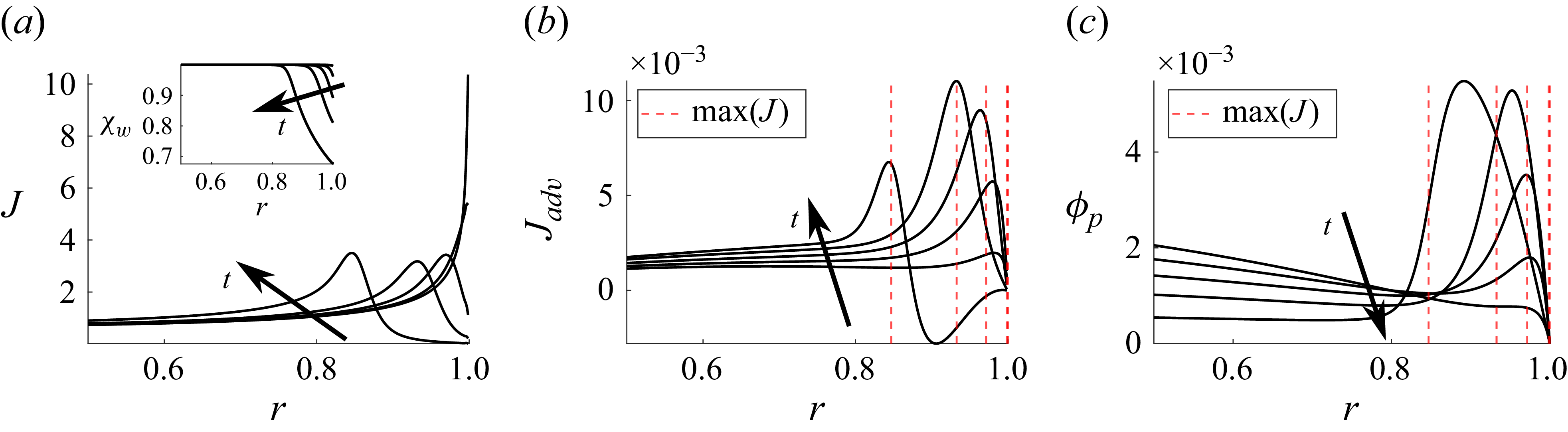
 t=tev,w×(0.1,0.3,0.5,0.7,0.9)
 Ca=10−4
 Pe=13.2
 wp0=3×10⁻³
 Hr=0.7
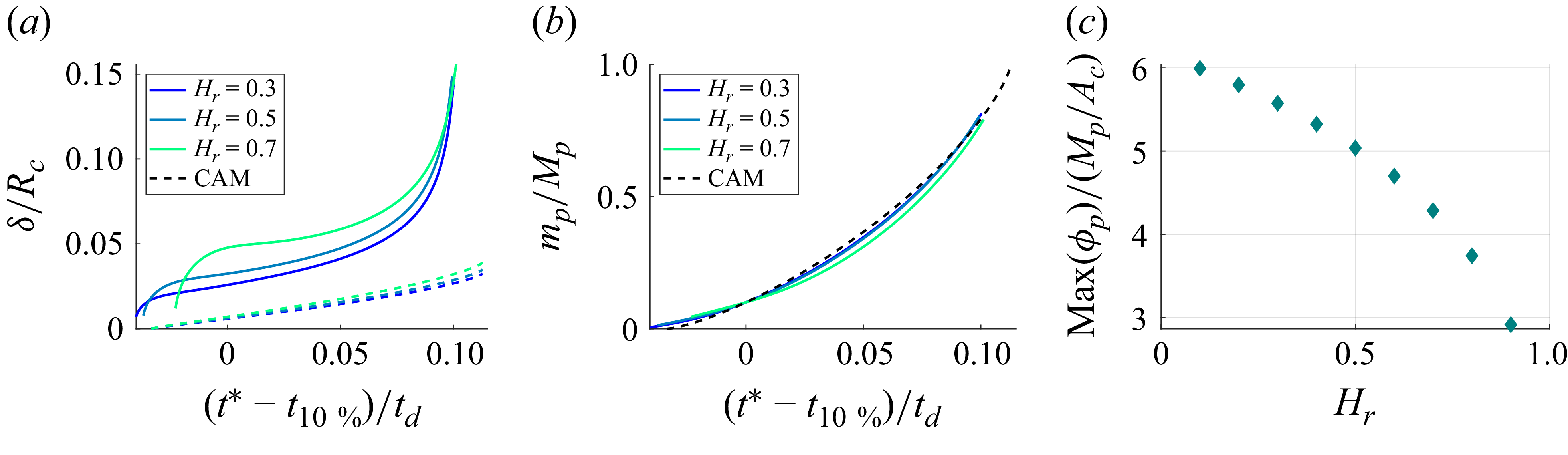
 Ac
 Ca=10−4
 Pe=43.3(1−Hr)
 wp0=3×10⁻³
 Hr=0.3,0.5,0.7
 t=tev,w
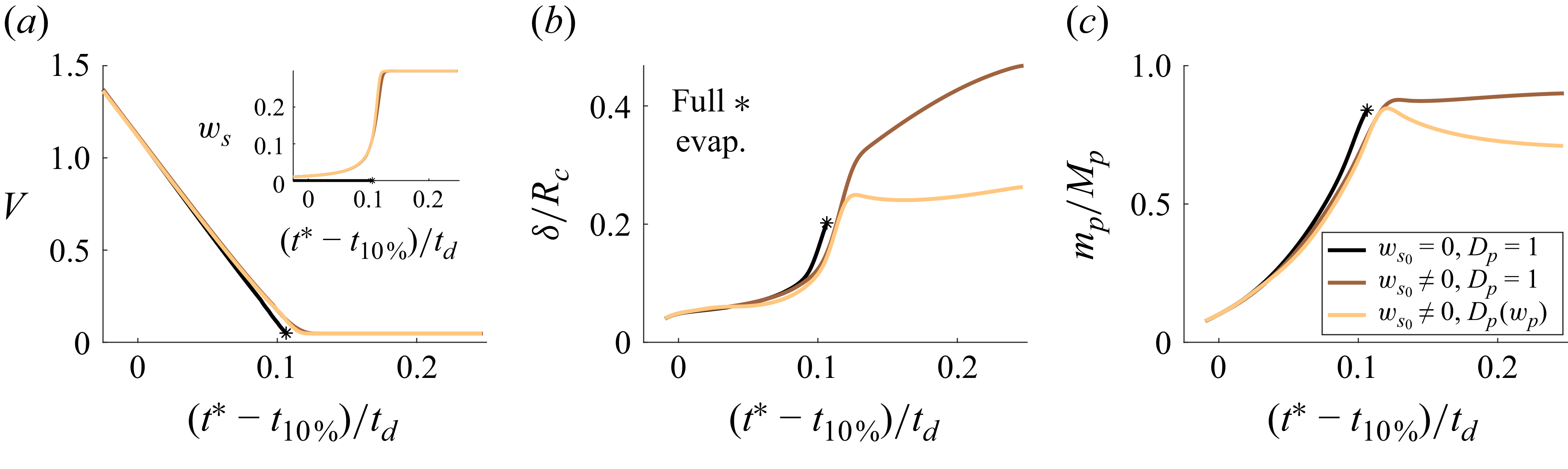
 Ca=10−4
 Pe=13.2
 wp0=3×10⁻³
 Hr=0.7
 ws0=0,9×10⁻³
 Dp=1
 D(wp)
 t=2tev,w
 ws0=9×10⁻³
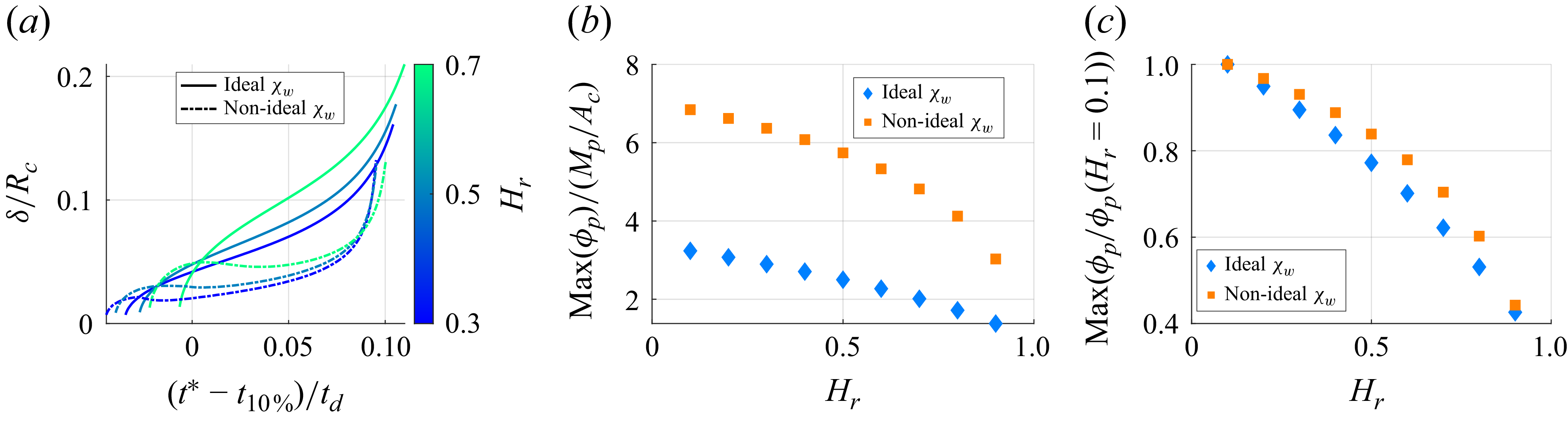
 χwp=1−wp
 Ac
 Ca=10−4
 Pe=43.3(1−Hr)
 wp0=3×10⁻³
 Hr=0.3,0.5,0.7
 t=tev,w

 Ca=10−4
 Pe=43.3(1−Hr)
 Hr=0.3,0.5,0.7
 D(wp)
 wp0=3×10⁻³
 ws0=9×10⁻³
 ws=0.25

 Ca=10−4
 Pe=43.3(1−Hr)
 Hr=0.3,0.4,0.5,0.6,0.7
 D(wp)
 wp0=3×10⁻³
 ws0=9×10⁻³
 ws=0.25

 Ac
 Ca=10−4
 Pe=43.3(1−Hr)
 wp0=3×10⁻³
 wp0=12×10−3
 t=tev,w

 Hr=30.4%
 T=20.5∘
 Hr=44.9%
 T=23.6∘
 Hr=67.4
 T=25.7∘
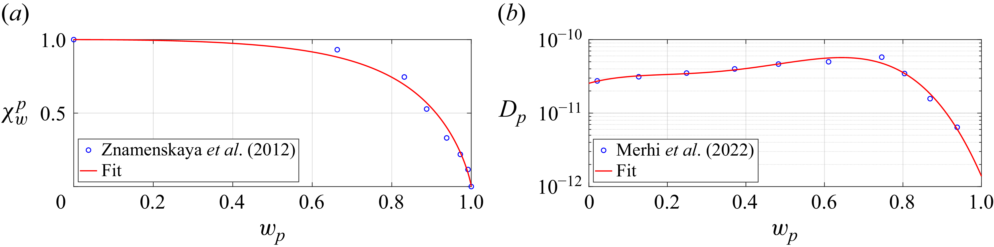

 Xwp
 Hr=0.3
 Ca=10−4
 Pe=43.3(1−Hr)
 Hr=0.3,0.5,0.7
 D(wp)
 wp0=3×10⁻³
 ws0=9×10⁻³
 ws=0.25

 Hr=0.3
 Hr=0.7
 Hr=0.3,0.7
 Ca=10−4
 Pe=43.3(1−Hr)
 D(wp)
 wp0=3×10⁻³
 ws0=9×10⁻³
 ws=0.25
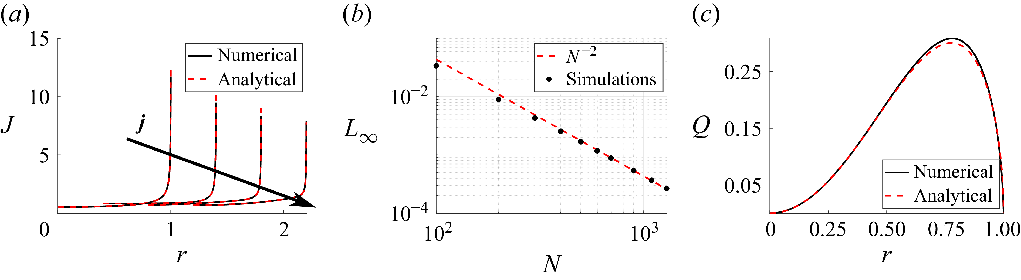
 j=0,2,4,6
 L∞
 Ca=10−4
 Pe=10
 Hr=0.5
 t=0.1
 χw≈1

 Open access

