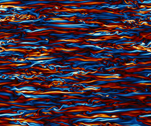



1. Introduction
In the turbulent flows of the atmosphere and ocean, buoyancy forces and stable stratification restrict vertical motion. At sufficiently small scales, the effects due to rotation are minor: stratification dominates these scales while Coriolis forces are weak (e.g. Riley & Lindborg Reference Riley, Lindborg, Davidson, Kaneda and Sreenivasan2013). Fluid velocities in stratified turbulence are approximately horizontal and layers containing quasi-two-dimensional vortices develop (e.g. Riley & Lelong Reference Riley and Lelong2000), along with gravity waves (e.g. Staquet & Sommeria Reference Staquet and Sommeria2002). At very small scales, fluctuations of variable fields (e.g. velocity, vorticity, density, temperature, etc.) are smoothed out by viscosity and buoyancy diffusivity, which typically occur at different inner scales. Direct numerical simulations (DNS) of stratified turbulence require that the smallest features are resolved, necessitating adequately fine grid spacing. The computational cost for these DNS is often reduced by setting the smoothing processes to be equally strong, but is done at the expense of misrepresenting the two disparate inner scales.
The relative strength of viscosity and buoyancy diffusivity is quantified by the dimensionless Prandtl number
 \begin{equation} Pr \equiv \nu/\kappa, \end{equation}
for kinematic viscosity  $\nu$ and thermal diffusivity
 $\kappa$, with temperature as the buoyancy-influenced scalar. Typical values for
 $\textit {Pr}$ are 0.7 for heat in air and 7 for heat in water; for salinity in water the analogous Schmidt number for the ratio of viscosity to mass diffusivity is about 700. We use
 $\textit {Pr}$ in this paper to refer to this ratio. Using large
 $\textit {Pr}$ values for DNS is computationally expensive: since buoyancy diffusivity can be several times weaker than viscous diffusion, the smallest temperature fluctuations can be reduced to extremely small scales, demanding high spatial resolution. By setting
 $\textit {Pr}=1$, the equally strong viscous dissipation and buoyancy diffusivity forces the two inner scales to coincide, relaxing the need for high resolution. Stratified turbulence dynamics could be sensitive to
 $\textit {Pr}$, but the
 $\textit {Pr} \neq 1$ problem has not been studied in depth for forced homogeneous stratified turbulence with no mean shear. In this paper, we investigate the effect of varying
 $\textit {Pr}$ in numerical simulations of homogeneous stratified turbulence, therefore additionally evaluating the suitability for
 $\textit {Pr}=1$ simulations to reproduce
 $\textit {Pr} \neq 1$ results.
Stratified turbulence is characterized by several length scales and dimensionless numbers, which we begin to review here (e.g. Riley & Lelong Reference Riley and Lelong2000; Davidson Reference Davidson2013; Riley & Lindborg Reference Riley, Lindborg, Davidson, Kaneda and Sreenivasan2013). The Kolmogorov microscale
 \begin{equation} k_d \equiv (\epsilon_k/\nu^3)^{1/4}, \end{equation}
with kinetic energy dissipation rate  $\epsilon _k$, is the inner scale of velocity fluctuations where kinetic energy is viscously dissipated into heat (Kolmogorov Reference Kolmogorov1941). Analogous to the viscous dissipation scale, the temperature fluctuations,
 $\theta$, have an inner scale (Corrsin Reference Corrsin1951; Tennekes & Lumley Reference Tennekes and Lumley1972)
 \begin{equation} k_{\theta} \equiv (\epsilon_k/\kappa^3)^{1/4}, \end{equation}
for thermal diffusion. There is also the Batchelor scale for the inner scale that describes passive scalar fluctuations (Batchelor Reference Batchelor1959; Davidson Reference Davidson2015),
 \begin{equation} k_B \equiv (\epsilon_k/ \nu \kappa^2)^{1/4}. \end{equation}
These two inner temperature scales are related by
 \begin{equation} k_{\theta}/k_B = (\nu/\kappa)^{1/4} = Pr^{1/4}. \end{equation}
Depending on the size of  $\textit {Pr}$, either
 $k_{\theta }$ or
 $k_B$ describes the dissipation scale for potential energy. When
 $\textit {Pr} \lesssim 1$,
 $k_{\theta }$ is most applicable, and when
 $\textit {Pr} \gg 1$,
 $k_B$ is most applicable (Wyngaard Reference Wyngaard2010; Gotoh & Yeung Reference Gotoh, Yeung, Davidson, Kaneda and Sreenivasan2013). When
 $\textit {Pr}>1$, we have that
 $k_{\theta }>k_d$, meaning that viscosity will begin to destroy velocity fluctuations at a scale where buoyancy diffusivity will not yet be effective. This subrange
 $k\in [k_d,k_{\theta }]$ is referred to as the viscous–convective subrange. If
 $\textit {Pr} \gg 1$, theory suggests that in the viscous–convective subrange, the potential energy spectrum has the form
 \begin{equation} E_P \sim \epsilon_p (\epsilon_k/\nu)^{-1/2} k^{-1}, \end{equation}
with potential energy dissipation rate  $\epsilon _p$, as predicted by Batchelor (Reference Batchelor1959). In the opposite case when
 $\textit {Pr}<1$, buoyancy diffusivity will act on small scales where viscous effects are not yet significant, and the subrange
 $k \in [k_{\theta },k_d]$ is the inertial–diffusive subrange (Wyngaard Reference Wyngaard2010). In the atmosphere, these inner scales typically correspond to lengths of the order of millimetres.
The buoyancy frequency  $N$ characterizes stratification strength: for temperature stratification,
 \begin{equation} N^2 \equiv \frac{g}{\theta_0} \beta, \end{equation}
where  $g$ is gravitational acceleration,
 $\theta _0$ is a reference temperature and
 $\beta$ is the background potential temperature gradient (e.g. Kundu, Cohen & Dowling Reference Kundu, Cohen and Dowling2012). The potential energy dissipation rate can be related to the diffusion of temperature fluctuations by
 \begin{equation} \epsilon_p =\frac{g/\theta_0}{\beta} \kappa \overline{\frac{\partial \theta}{\partial x_j} \frac{\partial \theta}{\partial x_j}}, \end{equation}
where  $\bar {(\cdot )}$ denotes a mean quantity.
The  $\textit {Pr} \neq 1$ problem in strongly stratified turbulence becomes complicated by the horizontally layered structure of the flow. In stratified turbulence, quasi-two-dimensional vortices become thinner with stronger stratification (Billant & Chomaz Reference Billant and Chomaz2001), introducing additional small scales that must be adequately resolved in DNS. The horizontal Froude number
 \begin{equation} Fr_h=U/N L_h , \end{equation}
for root mean square (r.m.s.) velocity  $U$ and horizontal length scale
 $L_h$, is a dimensionless number that quantifies stratification strength in stratified turbulence (Billant & Chomaz Reference Billant and Chomaz2001; Brethouwer et al. Reference Brethouwer, Billant, Lindborg and Chomaz2007). While turbulence is characterized by a large Reynolds number
 \begin{equation} Re = UL_h/\nu, \end{equation}
stratified turbulence can fall into one of two regimes depending on its buoyancy Reynolds number (Smyth & Moum Reference Smyth and Moum2000; Riley & de Bruyn Kops Reference Riley and de Bruyn Kops2003; Brethouwer et al. Reference Brethouwer, Billant, Lindborg and Chomaz2007)
 \begin{equation} Re_b=Re Fr_h^2. \end{equation}
Typical mesoscale flows (e.g. squall lines and sea breezes) have tropospheric values  $U \sim 1\ \mathrm {m}\,\mathrm {s}^{-1}$,
 $L_h \sim 1\text {--}100\ \mathrm {km}$,
 $N \sim 10^{-2}\ \mathrm {s}^{-1}$, and
 $\nu \sim 10^{-5}\ \mathrm {m}^2\,\mathrm {s}^{-1}$, giving ranges of dimensionless numbers
 $Fr_h \sim 10^{-3}\text {--}10^{-1}$,
 $\textit {Re} \sim 10^8\text {--}10^{10}$ and
 $\textit {Re}_b \sim 10^4\text {--}10^{6}$ (e.g. Lilly Reference Lilly1983; Waite Reference Waite2013). From the approximation
 $\epsilon _k \sim U^3/L_h$ (e.g. Taylor Reference Taylor1935; Lindborg Reference Lindborg2006), these values give a corresponding
 $\epsilon _k \sim 10^{-5}\text {--}10^{-3}\ \mathrm {m}^2 \,\mathrm {s}^{-3}$ (similar to dissipation values in the stratosphere, e.g. Dewan Reference Dewan1997).
Stratified turbulence also has the buoyancy scale
 \begin{equation} k_b \equiv N/U, \end{equation}
and Ozmidov scale
 \begin{equation} k_O \equiv (N^3/\epsilon_k)^{1/2}, \end{equation}
which characterize different small-scale processes in the flow. The thickness of the horizontal layers in stratified turbulence, and thus the largest vertical overturning scale corresponds to  $k_b$ (Billant & Chomaz Reference Billant and Chomaz2001; Carnevale, Briscolini & Orlandi Reference Carnevale, Briscolini and Orlandi2001; Waite & Bartello Reference Waite and Bartello2004). The Ozmidov scale is the largest scale for which the flow resembles small-scale three-dimensional isotropic turbulence (Ozmidov Reference Ozmidov1965). Whether
 $k_O$ is upscale or downscale of the dissipation range depends on the regime of stratified turbulence, such that
 \begin{equation} k_d / k_O \sim Re_b^{3/4}, \end{equation}
using the  $\epsilon _k \sim U^3/L_h$ assumption (Lindborg Reference Lindborg2006; Maffioli & Davidson Reference Maffioli and Davidson2016).
Past investigations that set  $\textit {Pr}=1$ revealed important properties of stratified turbulence and confirmed various scaling arguments. Stratified turbulence has two regimes: on the scale of the thickness of the quasi-two-dimensional vortices, viscosity may be weak enough that small eddies may emerge and the layers are turbulently coupled (characterized by
 $\textit {Re}_b>1$), or viscosity may be strong enough that the layers are non-turbulent and become viscously coupled (characterized by
 $\textit {Re}_b<1$) (Riley & de Bruyn Kops Reference Riley and de Bruyn Kops2003; Brethouwer et al. Reference Brethouwer, Billant, Lindborg and Chomaz2007). Within the horizontal layers, Kelvin–Helmholtz (KH) instabilities emerge when
 $\textit {Re}_b \gtrsim 1$ and break down into small-scale turbulence (Lilly Reference Lilly1983; Laval, McWilliams & Dubrulle Reference Laval, McWilliams and Dubrulle2003; Riley & de Bruyn Kops Reference Riley and de Bruyn Kops2003; Brethouwer et al. Reference Brethouwer, Billant, Lindborg and Chomaz2007; Waite Reference Waite2011). The kinetic and potential energy spectra in terms of horizontal wavenumber
 $k_h$ and vertical wavenumber
 $k_v$ have been extensively examined in studies with stratified turbulence simulations. Forced simulation results have shown the horizontal kinetic and potential energy spectra to exhibit
 $k_h^{-5/3}$ scaling (Brethouwer et al. Reference Brethouwer, Billant, Lindborg and Chomaz2007; Almalkie & de Bruyn Kops Reference Almalkie and de Bruyn Kops2012). In some instances, there is a noticeable bump at
 $k_h \sim k_b$ due to KH instabilities (Laval et al. Reference Laval, McWilliams and Dubrulle2003; Brethouwer et al. Reference Brethouwer, Billant, Lindborg and Chomaz2007; Waite Reference Waite2011). In the limit of strong stratification, the one-dimensional horizontal wavenumber spectra for kinetic and potential energy (where
 $k_h$ is the wavenumber magnitude in either the
 $x$- or
 $y$-direction, as in Lindborg & Brethouwer Reference Lindborg and Brethouwer2007) resemble
 \begin{gather} E_K(k_h) = C_1 \epsilon_k^{2/3}k_h^{-5/3}, \end{gather}
 \begin{gather}E_P(k_h) = C_2 \frac{\epsilon_p}{\epsilon_k^{1/3}} k_h^{-5/3}, \end{gather}
where  $C_1$ and
 $C_2$ are the Kolmogorov and Obukhov–Corrsin constants. The present work uses the two-dimensional horizontal wavenumber: the corresponding constants for the two-dimensional spectra,
 $C'_1$ and
 $C'_2$, are related to the one-dimensional values by
 $C' \approx 1.40 C$, for which Lindborg (Reference Lindborg2006) and Brethouwer et al. (Reference Brethouwer, Billant, Lindborg and Chomaz2007) use
 $C'_1 = C'_2 = 0.71$ as a reference value for their simulation results.
Scaling arguments have suggested  $k_v^{-3}$ scaling for the vertical kinetic and potential energy spectra for a limited range of wavenumbers (Billant & Chomaz Reference Billant and Chomaz2001; Lindborg Reference Lindborg2006); simulations have exhibited similarly steep vertical spectra past
 $k_b$ (Waite & Bartello Reference Waite and Bartello2004; Brethouwer et al. Reference Brethouwer, Billant, Lindborg and Chomaz2007; Almalkie & de Bruyn Kops Reference Almalkie and de Bruyn Kops2012). The behaviour of vertical spectra is scale dependent: at large horizontal scales, agreement with
 $k_v^{-3}$ scaling was shown for both kinetic and potential energy, but for different ranges of wavenumbers in simulations forced at large scales (Maffioli Reference Maffioli2017). Decaying simulations also supported the horizontal
 $k_h^{-5/3}$ scaling for kinetic and potential energy found in forced simulations (Bartello & Tobias Reference Bartello and Tobias2013; Maffioli & Davidson Reference Maffioli and Davidson2016), and were not influenced by stratification strength for large
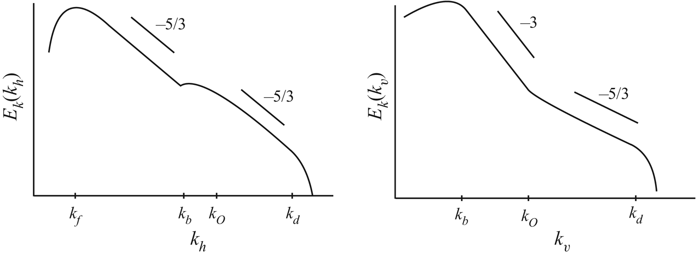
 $\textit {Re}$ (Lindborg Reference Lindborg2006; Bartello & Tobias Reference Bartello and Tobias2013). The conversion from potential to kinetic energy can be quantified by the buoyancy flux term in the energy budget (Holloway Reference Holloway1988; Waite Reference Waite2014). In the buoyancy flux spectrum, restratification describes the small-scale subrange with positive buoyancy flux, where potential energy is converted to vertical kinetic energy, restratifying the flow (Holloway Reference Holloway1988; Bouruet-Aubertot, Sommeria & Staquet Reference Bouruet-Aubertot, Sommeria and Staquet1996; Carnevale et al. Reference Carnevale, Briscolini and Orlandi2001). The relationship between the characteristic wavenumbers and spectral scaling laws is summarized in figure 1.
A schematic diagram of the expected spectral scaling laws and characteristic wavenumbers for stratified turbulence with  $Fr_h \ll 1$,
 $\textit {Re}_b \gg 1$ and
 $\textit {Pr}=1$.

Stratified turbulence with  $\textit {Pr}>1$ has not been as well studied as the
 $\textit {Pr}=1$ case, but previous studies have analysed such simulations with some compromises in other simulation parameters. Comparisons of decaying stratified turbulence DNS with
 $\textit {Pr}=7$ and
 $\textit {Pr}=700$ revealed
 $\textit {Pr}$-dependence in the energy spectra (Okino & Hanazaki Reference Okino, Hanazaki, Resch, Bez, Focht, Gienger and Kobayashi2017, Reference Okino and Hanazaki2019, Reference Okino and Hanazaki2020). The
 $\textit {Pr}=700$ potential energy spectra initially exhibited
 $k^{-1}$ scaling at large wavenumbers (as predicted in the viscous–convective subrange for passive scalars Batchelor Reference Batchelor1959), and by the final decay period, a flat spectrum developed in the dissipation range. However, the initial Reynolds number in this study was necessarily small (initial
 $\textit {Re}_0=50$) to accommodate the very large
 $\textit {Pr}$, limiting the extent of the inertial range; while small-scale changes due to
 $\textit {Pr}$ have been identified, it is also of interest to determine any possible
 $\textit {Pr}$-dependence upscale of the dissipation range. In Okino & Hanazaki (Reference Okino and Hanazaki2019), more DNS of decaying stratified turbulence were performed with a larger initial Reynolds number
 $\textit {Re}_0=100$ (corresponding to a microscale Reynolds number of
 $\textit {Re}_{\lambda }=42$) for
 $\textit {Pr}= 1$, 7 and 70. Each decaying DNS had an initial buoyancy Reynolds number of approximately 50 which quickly dropped to
 $\textit {Re}_b \sim 1$ within the first quarter of the simulation. A
 $k^{-1}$ power law region is again observed in the horizontal and vertical potential energy spectra for the largest
 $\textit {Pr}$ (70 in this study) early in the simulation before any significant decay. The authors note less of a difference in kinetic energy spectra between
 $\textit {Pr}=7$ and
 $\textit {Pr}=70$ than the difference between
 $\textit {Pr}=1$ and
 $\textit {Pr}=7$. An older study which performed DNS of stably stratified homogeneous turbulent shear flow concluded higher-
 $\textit {Pr}$ flows were more likely to exhibit counter-gradient heat flux (i.e. restratification) in the vertical direction, but their moderate
 $\textit {Re}$ limits its applicability to geophysical flows (Gerz, Schumann & Elghobashi Reference Gerz, Schumann and Elghobashi1989). Another study where DNS of density-stratified turbulent wakes were performed for
 $\textit {Pr}=0.2$, 1 and 7 concluded that using the
 $\textit {Pr}=1$ case to approximate the
 $\textit {Pr}=7$ case was reasonable, though the grid spacing was four times the smallest length scale of the flow (de Stadler, Sarkar & Brucker Reference de Stadler, Sarkar and Brucker2010). The
 $\textit {Pr}=7$ case induced small-scale changes with little influence on the wake's large-scale features, and the differences between the
 $\textit {Pr}=1$ and
 $\textit {Pr}=7$ cases were small compared to the substantial difference in computational costs. Mixing efficiency, which is often studied in DNS with
 $\textit {Pr}=1$ (e.g. Caulfield & Peltier Reference Caulfield and Peltier2000; Maffioli, Brethouwer & Lindborg Reference Maffioli, Brethouwer and Lindborg2016; Howland, Taylor & Caulfield Reference Howland, Taylor and Caulfield2020), has been found to decrease with increasing
 $\textit {Pr}$ (Smyth, Moum & Caldwell Reference Smyth, Moum and Caldwell2001; Stretch et al. Reference Stretch, Rottman, Venayagamoorthy, Nomura and Rehmann2010; Salehipour, Peltier & Mashayek Reference Salehipour, Peltier and Mashayek2015). In comparison, the dependence of mixing efficiency on stratification strength and the Richardson number is more complicated (Peltier & Caulfield Reference Peltier and Caulfield2003; Howland et al. Reference Howland, Taylor and Caulfield2020).
In this work, we address the following question: in DNS of stratified turbulence with  $Fr_h < 1$, is the dynamics at scales of the order of the Ozmidov and Kolmogorov scales and larger independent of
 $\textit {Pr}$ for
 $\textit {Re}_b \sim O(10)$? Or put another way: are DNS with
 $\textit {Pr}=1$ able to reproduce results with
 $\textit {Pr}>1$, at least at large scales? Many DNS studies of stratified turbulence consider
 $\textit {Re}_b \lesssim O(10)$, especially with strong stratification (e.g. Kimura & Herring Reference Kimura and Herring2012; Bartello & Tobias Reference Bartello and Tobias2013; Maffioli Reference Maffioli2017; Okino & Hanazaki Reference Okino and Hanazaki2019), and many of these studies set
 $\textit {Pr}=1$; answering this question will shed light on the applicability of their results to
 $\textit {Pr} > 1$ flows. Since varying
 $\textit {Pr}$ affects the relative strengths of small-scale processes, we anticipate that most
 $\textit {Pr}$-induced changes will occur around the small viscous dissipation and buoyancy diffusion scales. If the viscosity is held fixed while
 $\textit {Pr}$ is increased, we would also predict that changes in the temperature and potential energy would be more pronounced than in the velocity and kinetic energy. Further, for fixed viscosity, the dissipation of potential energy (or of temperature fluctuations, as in (1.8)) is expected to be especially
 $\textit {Pr}$-sensitive as
 $k_B$ is modified. Equation (1.14) expresses a scale separation in stratified turbulence in terms of the characteristic
 $\textit {Re}_b$, suggesting that sensitivity to
 $\textit {Pr}$ may depend on the regime of stratified turbulence. Indeed, for
 $\textit {Re}_b \lesssim 1$, stratified turbulence is dominated by large, thin, viscously coupled layers, and therefore large horizontal scales are affected directly by viscous dissipation (e.g. Brethouwer et al. Reference Brethouwer, Billant, Lindborg and Chomaz2007) and may be sensitive to
 $\textit {Pr}$. As a small-scale phenomenon involving potential energy, restratification is another candidate for
 $\textit {Pr}$-dependence. Due to the complicated dependence of buoyancy flux on the stratification strength, varying
 $\textit {Pr}$ may also affect the restratification range in regime-specific ways (Lucas, Caulfield & Kerswell Reference Lucas, Caulfield and Kerswell2017).
In this paper, DNS of homogeneous forced stratified turbulence are performed and analysed to explore the effect of varying  $\textit {Pr}$ on the flow dynamics. The choices of
 $\textit {Pr}$ and stratification span a range of
 $\textit {Re}_b$ so that the
 $\textit {Re}_b=1$ stratified turbulence regime transition may also be studied. In § 2, the numerical model, equations, and set-up of simulations are explained. In § 3, the simulation results are analysed in terms of scale-specific observations of
 $\textit {Pr}$-dependence in the energy spectra, buoyancy flux spectra, spectral energy flux and snapshots of physical space fields. Conclusions, discussion and future work are given in § 4.
2. Methods
2.1. Equations and model
For the stratified turbulence simulations presented here, the governing equations are the incompressible uniformly stratified non-rotating Boussinesq equations in three dimensions
 \begin{gather} \frac{\mathrm{D}\boldsymbol{u}}{\mathrm{D} t} = - \boldsymbol{\nabla} p + \alpha \theta {\hat{\boldsymbol{z}}}+ \boldsymbol{F}_u + \nu \nabla^2 \boldsymbol{u}, \end{gather}
 \begin{gather}\frac{\mathrm{D} \theta}{\mathrm{D} t} + \beta w = F_b + \kappa \nabla^2 \theta, \end{gather}
 \begin{gather}\boldsymbol{\nabla} \boldsymbol{\cdot} \boldsymbol{u} = 0, \end{gather}
where  $\boldsymbol {u}$ is velocity,
 $p$ is pressure scaled by a reference density,
 $\theta$ is the potential temperature fluctuation (or negative density fluctuation),
 $\hat {\boldsymbol {z}}$ is the upward vertical unit vector,
 $\boldsymbol {F}_{u}$ is the velocity forcing,
 $F_b$ is the temperature forcing,
 $\nu$ is viscosity,
 $\kappa$ is diffusivity,
 $\alpha$ is thermal expansivity and
 $\beta$ is the background potential temperature gradient (Herring & Métais Reference Herring and Métais1989).
The DNS code computes the fluid velocity by first solving for vorticity ( $\boldsymbol {\omega }=\boldsymbol {\nabla } \times \boldsymbol {u}$) from the vorticity formulation of (2.1)
 \begin{equation} \frac{\partial \boldsymbol{\omega}}{\partial t} = \boldsymbol{\nabla} \times ( \boldsymbol{u} \times \boldsymbol{\omega}) + \alpha \left[ \begin{array}{@{}c@{}} \partial \theta / \partial y \\ - \partial\theta / \partial x \\ 0 \end{array} \right] + \boldsymbol{F}_{\omega} + \nu \nabla^2 \boldsymbol{\omega} \end{equation}
and (2.2), then inverting the result for  $\boldsymbol {u}$. This inversion assumes no mean velocity. In this formulation, the second term on the right-hand side of (2.4) corresponds to the baroclinic generation of vorticity, and
 $\boldsymbol {F}_{\omega }=\boldsymbol {\nabla } \times \boldsymbol {F}_{u}$ is the vorticity forcing.
The spectral transform method is used on a triply periodic domain to solve the uniformly stratified Boussinesq equations (2.2), (2.3), and (2.4). The domain is a cube of size  $L \times L \times L$ and grid size
 $n \times n \times n$ in both the physical and Fourier domains where
 $\boldsymbol {u}$,
 $\boldsymbol {\omega }$ and
 $\theta$ are stored. Nonlinear terms are computed in the physical domain, and spatial derivatives are computed in the Fourier domain, and a fast Fourier transform is used to go between domains (Frigo & Johnson Reference Frigo and Johnson2005). Third-order Adams–Bashforth time stepping is used with constant time step
 ${\rm \Delta} t$, and viscous and diffusive terms use a Crank–Nicolson scheme (Durran Reference Durran2010). Aliasing issues are countered by a less restrictive wavenumber truncation than the 2/3 rule, which is known to eliminate all aliasing error (Durran Reference Durran2010). Previous DNS studies have used wavenumber truncations as high as 15/16, which still managed to remove the dominant aliasing error (Riley & de Bruyn Kops Reference Riley and de Bruyn Kops2003). In the following simulations, the Fourier coefficients are cubically truncated at a maximum wavenumber
 $k_{max}=({n}/{2}) ({8}/{9}) = 4n/9$. The effective resolution is then
 ${\rm \Delta} x = {\rm \Delta} y = {\rm \Delta} z = 9L/8n$ with wavenumber spacing
 ${\rm \Delta} k_x = {\rm \Delta} k_y = {\rm \Delta} k_z = 2 {\rm \pi} / L$. This model has been used in numerous studies of stratified turbulence, e.g. Waite (Reference Waite2011, Reference Waite2017) and Lang & Waite (Reference Lang and Waite2019).
The equations for the kinetic and potential spectral energy budget for each wavevector  $\boldsymbol {k}$ are (e.g. Wyngaard Reference Wyngaard2010; Riley & Lindborg Reference Riley, Lindborg, Davidson, Kaneda and Sreenivasan2013)
 \begin{gather} \frac{\partial E_K}{\partial t}(\boldsymbol{k}) = T_K(\boldsymbol{k}) + B(\boldsymbol{k}) - D_K(\boldsymbol{k}) + F(\boldsymbol{k}), \end{gather}
 \begin{gather}\frac{\partial E_P}{\partial t}(\boldsymbol{k}) = T_P(\boldsymbol{k}) - B(\boldsymbol{k}) - D_P(\boldsymbol{k}). \end{gather}
The first terms on the right-hand side of (2.5) and (2.6),
 \begin{gather} T_K(\boldsymbol{k}) \equiv -\mathrm{Im} \sum_{\boldsymbol{k}+\boldsymbol{p}+\boldsymbol{q}=0} P_{ijm}(\boldsymbol{k}) \hat{u}_j(\boldsymbol{p}) \hat{u}_m(\boldsymbol{q}) \hat{u}_i(\boldsymbol{k}), \end{gather}
 \begin{gather}T_P(\boldsymbol{k}) \equiv - \frac{\alpha}{\beta} \mathrm{Im} \left( k_j \sum_{\boldsymbol{k}+\boldsymbol{p}+\boldsymbol{q}=0} \hat{\theta}(\boldsymbol{k}) \hat{\theta}(\boldsymbol{p}) \hat{u}_j (\boldsymbol{q}) \right), \end{gather}
are the nonlinear kinetic and potential energy transfer respectively, using the standard projection operator  $P_{ijm}$ (e.g. Rose & Sulem Reference Rose and Sulem1978). The spectral buoyancy flux,
 $B$, is
 \begin{equation} B(\boldsymbol{k}) \equiv \alpha\,{Re} ( \hat{\theta}(\boldsymbol{k}) \hat{w}^*(\boldsymbol{k}) ), \end{equation}
the kinetic and potential energy dissipation are
 \begin{gather} D_K(\boldsymbol{k}) \equiv 2 \nu k^2 E_K(\boldsymbol{k}), \end{gather}
 \begin{gather}D_P(\boldsymbol{k}) \equiv 2 \kappa k^2 E_P(\boldsymbol{k}), \end{gather}
and  $F$ is the forcing. Horizontal and vertical wavenumber spectral budgets are found from (2.5) and (2.6) by summing over all wavevectors
 $\boldsymbol {k}$ for particular horizontal wavenumber
 $k_h$ or vertical wavenumber
 $k_v$.
The spectral buoyancy flux  $B$ is the cross spectrum of buoyancy and vertical velocity, and can be interpreted as the transfer of potential to kinetic energy (e.g. Holloway Reference Holloway1988). Holloway (Reference Holloway1988) suggested that restratification, i.e. positive
 $B$ at small scales, occurs because the downscale transfer of potential energy to small scales was more efficient than for kinetic energy, leading to a tendency for more potential energy than kinetic energy to accumulate at small scales. Oppositely, when only kinetic energy is forced, more kinetic energy would accumulate at large scales than potential energy, and so these imbalances drive the conversion of kinetic to potential energy at large scales (
 $B<0$) and potential to kinetic energy at small scales (
 $B>0$, restratification).
The transfer terms represent the conservative transfer of potential and kinetic energy to different wavenumbers. Since they are conservative, the spectral fluxes of kinetic and potential energy are obtained from the transfer terms as
 \begin{gather} \varPi_K(k) = -\int_0^k T_K(k)\,\mathrm{d}k, \end{gather}
 \begin{gather}\varPi_P(k) = -\int_0^k T_P(k)\,\mathrm{d}k, \end{gather}
where  $k$ can be the isotropic, horizontal or vertical wavenumber magnitude. As conserved quantities, the transfer terms satisfy
 \begin{gather} \int_0^{\infty} T_K(k)\, \mathrm{d}k = 0, \end{gather}
 \begin{gather}\int_0^{\infty} T_P(k)\, \mathrm{d}k=0, \end{gather}
which also manifest as  $\varPi _K = 0$ and
 $\varPi _P = 0$ at
 $k_{max}$.
2.2. Simulation set-up
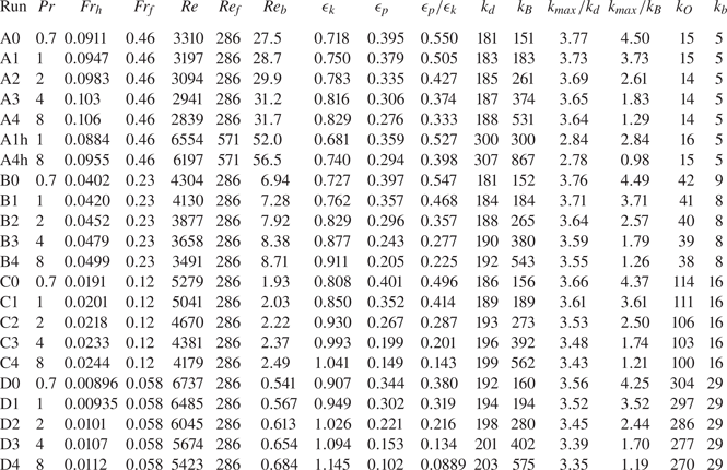
The parameter values, non-dimensional numbers and wavenumbers for all simulations presented here are given in table 1 and described here. Most simulations are performed on cubic domains with  $n=1536$ grid points in each direction. Two additional higher-resolution simulations, A1h and A4h, use
 $n=1920$.
Simulation parameters, non-dimensional numbers and wavenumbers for all simulations. The run label letter A/B/C/D indicates a common stratification strength. The run label number 0/1/2/3/4 indicates a common Prandtl number. All simulations have the same viscosity, resolution and maximum wavenumber:  $\nu =0.12\ \textrm {cm}^{2}\,\textrm {s}^{-1}$,
 $n=1536$,
 $k_{max}=682$ with the exception of runs A1h and A4h where
 $\nu =0.06\ \textrm {cm}^{2}\,\textrm {s}^{-1}$,
 $n=1920$,
 $k_{max}=853$. Wavenumbers are non-dimensionalized by
 $2{\rm \pi} /L$; energy dissipation is non-dimensionalized by forcing power
 $P$.

Large-scale vortical motion is excited by directly forcing vortical modes, i.e. flow with rotational horizontal velocity and no vertical velocity (vortical mode forcing was also used by e.g. Waite & Bartello Reference Waite and Bartello2004; Lindborg Reference Lindborg2006; Brethouwer et al. Reference Brethouwer, Billant, Lindborg and Chomaz2007). Gravity waves are not directly forced. Time dependence of the forcing follows an AR(1) red noise process with a short decorrelation time scale of  $\tau =$ 10 time steps (i.e. nearly white noise, e.g. Waite Reference Waite2017),
 \begin{equation} G(\boldsymbol{k},t_n)=\tilde{\alpha} G(\boldsymbol{k},t_{n-1})+ \tilde{\beta} g (\boldsymbol{k},n), \end{equation}
for a random complex number  $g(\boldsymbol {k},n)$. The random number's real and imaginary parts follow a Gaussian distribution with a mean of 0 and variance of 1. The coefficients in (2.16) satisfy
 \begin{equation} \tilde{\alpha}=\exp(-{\rm \Delta} t/\tau), \quad \tilde{\beta}^2 = 1-\tilde{\alpha}^2. \end{equation}
A specified forcing amplitude  $A(\boldsymbol {k})$ multiplies
 $G(\boldsymbol {k},t_n)$ and is non-zero only in the spherical shell
 $k\in [3,5]$ centred on forcing wavenumber
 $k_f=4$. The amplitude is given by
 \begin{equation} A(\boldsymbol{k}) = \begin{cases} a(k_f+1-|\boldsymbol{k}|)(|\boldsymbol{k}|-k_f+1), & k_f-1 \le |\boldsymbol{k}| \le k_f+1 ,\\ 0, & ||\boldsymbol{k}|-k_f| > 1 . \end{cases} \end{equation}
The forcing injects kinetic energy only. The time-averaged rate of energy injection by the forcing is approximately determined by the forcing amplitude as
 \begin{equation} P = 2\tau \sum_{\boldsymbol{k}} A(\boldsymbol{k})^2 , \end{equation}
(see Waite (Reference Waite2017), who found that the time-averaged energy injection rate scaled like  $P$ when
 $\tau$ was short). Note, this forcing approach is different from that employed by Lindborg (Reference Lindborg2006), in which the instantaneous, not time-averaged, energy injection rate is fixed. The simulations are initialized with a prescribed kinetic and potential energy at a chosen wavenumber
 $k=3$. Damping is applied to the
 $k_h=0$ modes to prevent the accumulation of energy in vertically sheared horizontal flow (Smith & Waleffe Reference Smith and Waleffe2002). More details on the code used for these simulations can be found in past studies (Waite Reference Waite2011, Reference Waite2017).
The simulations are described with dimensional parameters  $L$,
 $\nu$,
 $N$, etc. as well as dimensionless parameters. The dimensional parameters are chosen to be broadly similar to laboratory values following Waite (Reference Waite2014):
 $L$ is set to be
 $2{\rm \pi}$ metres for convenience, and the forcing amplitude is chosen to give velocities of the order of
 $1 \ \textrm {cm}\,\textrm {s}^{-1}$ and energy dissipation rates of the order of
 $0.01\ \textrm {cm}^2\,\textrm {s}^{-3}$. The forcing amplitude is the same in all simulations, and gives
 $P = 0.02586 \ \textrm {cm}^2\,\textrm {s}^{-3}$, which yields a forcing eddy time scale of
 $T_f =P^{-1/3}k_f^{-2/3}$. Stratification is changed by varying
 $N$. Viscosity is fixed at
 $\nu =0.12\ \textrm {cm}^2\,\textrm {s}^{-1}$ in all simulations except for A1h and A4h. The quantities in table 1 are non-dimensionalized by
 $P$ and
 $k_f$ as in Lindborg (Reference Lindborg2006). Energy time series, energy dissipation time series, energy spectra and energy transfer spectra computed for each simulation are non-dimensionalized by
 $P$ and
 $k_f$. A Froude number can be defined from the forcing parameters:
 $Fr_f=(Pk_f^2)^{1/3}/N$ (note that we use
 $k_f$, not
 $k_f/2{\rm \pi}$, so our
 $Fr_f$ values are larger at the same stratification than those used by Lindborg Reference Lindborg2006). This forcing Froude number
 $Fr_f$ is reported in table 1 (
 $Fr_f = 0.46$, 0.23, 0.12, 0.058) in place of our dimensional
 $N$ values (
 $N=0.075\ \textrm {s}^{-1}$,
 $0.15\ \textrm {s}^{-1}$,
 $0.3\ \textrm {s}^{-1}$,
 $0.6\ \textrm {s}^{-1}$). A forcing Reynolds number,
 $\textit {Re}_f=P^{1/3}/\nu k_f^{4/3}$, is also reported in table 1. The total dissipation rate
 $\epsilon _k+\epsilon _p$ is approximately equal to (but slightly larger than)
 $P$ in all cases, consistent with Waite (Reference Waite2017), who found that the actual energy injection rate was a little larger than (1.1 times) that determined by the forcing amplitude.
The total integration length for all simulations corresponds to approximately 17.3 forcing eddy time scales, and the time step is  ${\rm \Delta} t/T_f = 0.000216$. Time series are used for the calculated values in table 1, based on values for
 $\epsilon _k$ and
 $\epsilon _p$ averaged over
 $t/T_f \in [10.4,17.3]$. The length scale used in
 $Fr_h$ and
 $\textit {Re}$ is computed from
 $L_h=U^3/\epsilon _k$, where
 $U$ is the root mean square velocity (as in Brethouwer et al. Reference Brethouwer, Billant, Lindborg and Chomaz2007). While questions have been raised about the appropriateness of this
 $L_h$ in stratified turbulence (e.g. Maffioli & Davidson Reference Maffioli and Davidson2016), we include the corresponding
 $Fr_h$ for comparison with other studies that used it. Velocity, vorticity and temperature fields in physical space are output at equidistant times over the integration length (either 5 or 9 output times depending on the case).
The first set of simulations has a fixed stratification, thus setting  $Fr_f$, and separate trials for each Prandtl number. This approach was repeated for a total of 4 stratification strengths and 5 Prandtl numbers, resulting in 20 simulations at the same resolution with
 $\textit {Pr}=0.7$, 1, 2, 4 and 8 (runs with labels 0, 1, 2, 3 and 4 respectively) and
 $Fr_f= 0.46$, 0.23, 0.12 and 0.058 (runs with labels A, B, C and D respectively). The stratification strengths were chosen to give a range of
 $Fr_h$, and values for
 $\textit {Re}_b$ of O(1) and larger. The resolution
 $n=1536$ ensures that the Kolmogorov and Batchelor scales are resolved (
 $k_{max}/k_d \approx 3$ and
 $k_{max} / k_B > 1$). While the forcing amplitude and viscosity are fixed in all the
 $n=1536$ runs, the mixing efficiency depends on
 $Fr_f$ and
 $\textit {Pr}$. As a result,
 $\epsilon _k$ and
 $k_d$ are also dependent on
 $Fr_f$ and
 $\textit {Pr}$. In addition to studying dependence on
 $\textit {Pr}$, these parameter values explore both regimes of strongly stratified turbulence,
 $\textit {Re}_b < 1$ and
 $\textit {Re}_b >1$. Two additional simulations, A1h and A4h, have the same stratification but larger
 $\textit {Re}$ and
 $\textit {Re}_b$ than the other A cases, and are discussed in § 3.3.
The horizontal and vertical kinetic energy spectra are (e.g. Waite & Bartello Reference Waite and Bartello2004)
 \begin{gather} E_K(k_h)\delta = \tfrac{1}{2}\sum_{\boldsymbol{k}' \in I_h(k_h)}|\hat{\boldsymbol{u}}(\boldsymbol{k}')|^2, \end{gather}
 \begin{gather}E_K(k_v)\delta = \tfrac{1}{2}\sum_{\boldsymbol{k}' \in I_v(k_v)}|\hat{\boldsymbol{u}}(\boldsymbol{k}')|^2, \end{gather}
where
 \begin{gather} I_h(k_h) = \{ \boldsymbol{k}' \mid k_h - \delta/2 \leq k'_h < k_h + \delta/2 \}, \end{gather}
 \begin{gather}I_v(k_v) = \{ \boldsymbol{k}' \mid k_v - \delta/2 \leq |k'_v| < k_v + \delta/2 \}, \end{gather}
 $\delta = 2{\rm \pi} /L$ and
 $\hat {\boldsymbol {u}}$ corresponds to the velocity in the Fourier domain. The horizontal and vertical potential energy spectra are similarly defined
 \begin{gather} {E_P(k_h)\delta = \tfrac{1}{2}\sum_{\boldsymbol{k}' \in I_h(k_h)} |\hat{b}(\boldsymbol{k}')|^2/N^2 ,} \end{gather}
 \begin{gather}{E_P(k_v)\delta = \tfrac{1}{2}\sum_{\boldsymbol{k}' \in I_v(k_v)}|\hat{b}(\boldsymbol{k}')|^2/N^2 ,} \end{gather}
where  $\hat {b}$ corresponds to the buoyancy in the Fourier domain.
3. Results
In this section, we analyse kinetic and potential energy spectra, spectral budget terms and physical space fields of the simulations. We start with  $\textit {Pr}=1$, first focusing on the
 $Fr_f=0.12$ case (§ 3.1.1), then we look at the effect of varying
 $Fr_f$ for the
 $\textit {Pr}=1$ cases (§ 3.1.2). In § 3.2 we analyse the spectra and snapshots for
 $\textit {Pr}$-dependence. In § 3.3 we briefly discuss the effect of further increasing
 $\textit {Re}_b$ on the present results.
3.1. Overview of  $\textit {Pr}=1$ cases

3.1.1. Overview of the $Fr_f=0.12$, $\textit {Pr}=1$ case


We start with an overview of the  $\textit {Pr}=1$ case with intermediate stratification
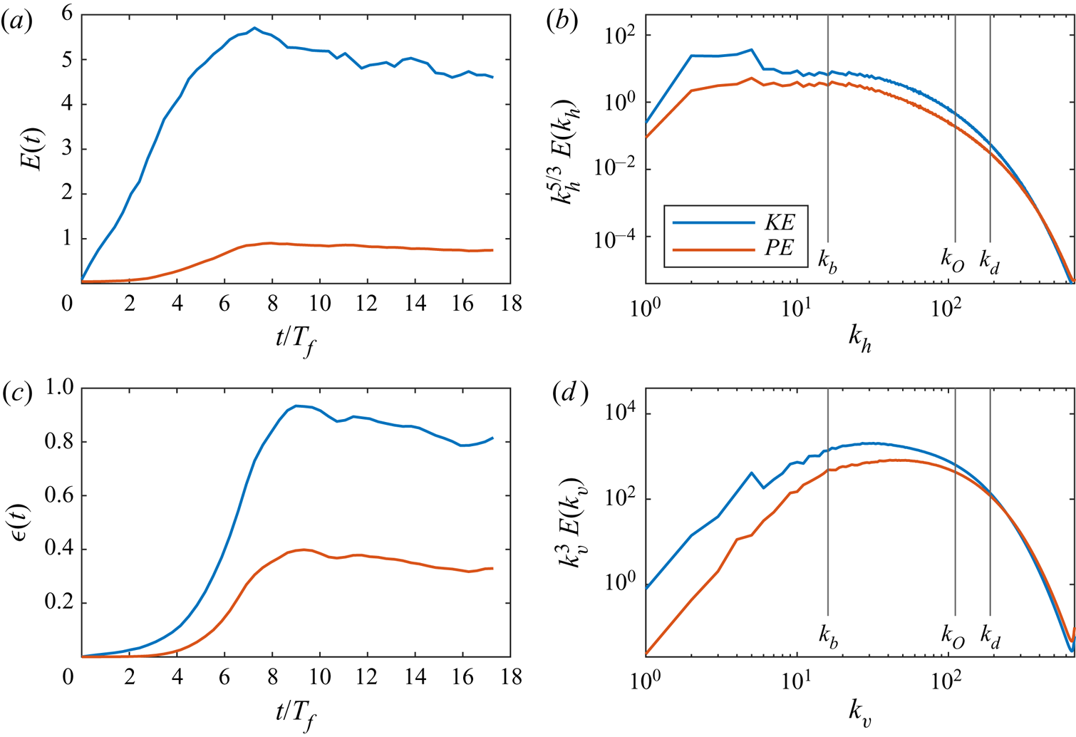
 $Fr_f=0.12$ (run C1). Time series of kinetic and potential energy and dissipation are plotted in figure 2(a,c). The energy and dissipation rates increase for the first 8 forcing time scales until the flow develops into statistically stationary turbulence, after which these quantities equilibrate. The energy and dissipation plots are fairly steady for
 $t/T_f\in [10.4,17.3]$, which is chosen as the time averaging interval. Approximate stationarity at these times is observed for all the simulations, so the same time averaging interval is used for all cases.
Energy spectra and time series for run C1:  $\textit {Pr}=1$,
 $Fr_f=0.12$. (a,c) Time series of (a) kinetic and potential energy and (c) kinetic and potential energy dissipation. (b,d) Compensated kinetic and potential energy spectra in terms of (b) horizontal and (d) vertical wavenumber. Characteristic wavenumbers
 $k_b$,
 $k_O$ and
 $k_d$ are denoted with vertical solid lines. Note that
 $k_B$ is coincident with
 $k_d$ for
 $\textit {Pr}=1$.

Compensated horizontal and vertical wavenumber spectra are plotted in figure 2(b,d) (the full wavenumber energy spectra are omitted as they closely resemble the vertical spectra). Spikes in the kinetic energy spectra for small wavenumbers are a consequence of the large-scale forcing for  $k\in [3,5]$. For
 $\textit {Pr}=1$,
 $k_d$ and
 $k_B$ (label omitted) are coincident. Beyond the forcing interval, the horizontal spectra are close to the expected
 $k_h^{-5/3}$ scaling law (Lindborg Reference Lindborg2006, represented by a plateau in the compensated spectra) for less than one decade, as expected for
 $\textit {Re}_b=2.03$. The uncompensated vertical kinetic energy spectrum is flat out to
 $k_b$ (not pictured in figure 2 but can be deduced by the approximate slope of
 $+3$ in the compensated plots), while the potential energy spectrum is peaked at
 $k_b$. Beyond
 $k_b$, the vertical spectrum steepens to approximately
 $k_v^{-3}$, appearing as a short plateau in the compensated plot. Due to the modest
 $\textit {Re}_b=2.03$ in this case, there is only a small separation between the Ozmidov and dissipation scales. Since
 $\textit {Pr}=1$, the kinetic and potential energy are expected to behave similarly at very small scales as both momentum– and buoyancy–diffusive scales are equivalent; indeed, in the dissipation range beyond
 $k_d$ (or
 $k_B$), the spectra are nearly the same.
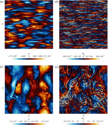
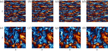
Figure 3 shows vertical and horizontal slices of horizontal velocity and vorticity at the end of the simulation. With  $\textit {Re}_b=2.03$ and
 $Fr_h=0.019$, run C1 is in the strongly stratified and slightly viscous regime where the flow is arranged into layers of pancake eddies. This run is only slightly past the
 $\textit {Re}_b=1$ transition from viscously to turbulently coupled layers. In figure 3(a,b), the layerwise arrangement and intermittent small-scale KH instabilities can be seen clearly in the vertical slices of the velocity and
 $y$-component vorticity fields. The buoyancy wavenumber
 $k_b=16$ for run C1 is approximately the number of layers in the flow. Since the thickness of the horizontal layers in stratified turbulence is set by the buoyancy length scale
 $L_b$ (Billant & Chomaz Reference Billant and Chomaz2001; Waite & Bartello Reference Waite and Bartello2004), the corresponding wavenumber
 $k_b=N/U= 2{\rm \pi} / L_b$ is approximately the number of layers in our domain of height
 $2{\rm \pi}$. The horizontal slices of velocity and
 $z$-component vorticity fields in figure 3(c,d) clearly show the signature of the large-scale vortical forcing. In addition, small horizontal scales associated with KH billows are visible in figure 3(d).
Vertical slices  $(x,z)$ at
 $y=0$ of (a)
 $x$-component velocity
 $u$ and (b)
 $y$-component vorticity
 $\omega _y$. Horizontal slices
 $(x,y)$ at
 $z=0$ of (c)
 $x$-component velocity
 $u$ and (d)
 $z$-component vorticity
 $\omega _z$. All fields are computed at the end of run C1. Numerical values on the colour bars correspond to dimensional quantities.

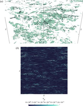
The potential energy dissipation field (1.8) is shown in figure 4. Run C1 has few regions that are highly dissipative, and in figure 4(a) the dissipative regions resemble small quasi-horizontal features in contrast with the intermittent worms expected in unstratified homogeneous three-dimensional turbulence (e.g. Burgers Reference Burgers, von Mises and von Kármán1948; Siggia Reference Siggia1981; Ishihara, Kaneda & Hunt Reference Ishihara, Kaneda and Hunt2013). These dissipative regions also appear to be arranged in horizontal layers (figure 4b), like the vertical slices of  $u$ and
 $\omega _y$ in figure 3(a,b).
Potential energy dissipation field,  $\epsilon _p$, computed at the end of run C1: (a) isosurfaces of 5 % of the maximum value, (b) vertical slice
 $(x,z)$ at
 $y=0$; numerical values on the colour bar correspond to dimensional quantities.

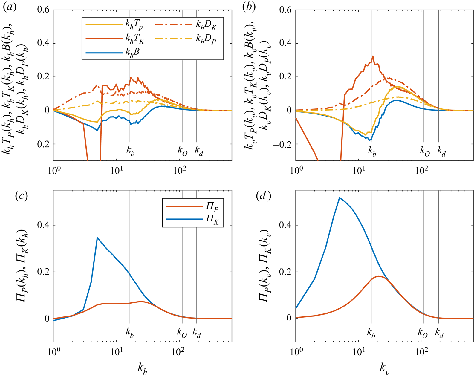
We now consider the spectral budget for run C1. The spectra of  $T_K$,
 $T_P$,
 $D_K$,
 $D_P$ and
 $B$ from the energy budget (2.5) and (2.6) are plotted for run C1 in figure 5(a,b). Excluding the dissipation terms, the horizontal and vertical spectral budgets are similar at large scales; the shape of the spectra at small wavenumbers is primarily influenced by the large-scale forcing. In the forcing interval, there is substantial transfer of the injected kinetic energy out of the forced wavenumbers, as indicated by large negative spikes in
 $T_K(k_h)$ and
 $T_K(k_v)$. The potential energy budget terms
 $T_P(k_h)$,
 $T_P(k_v)$,
 $B(k_h)$ and
 $B(k_v)$ are very small and negative in this range, indicating that, while there is no direct forcing of potential energy, there is some conversion of the remaining injected kinetic energy to potential energy.
(a,b) Spectra for kinetic and potential energy transfer terms, kinetic and potential energy dissipation and buoyancy flux for run C1. Spectra are multiplied by wavenumber to preserve area under the curve for linear–log axes. (c,d) Spectral energy fluxes for run C1.

In the horizontal spectral budget, downscale of the forcing interval,  $T_K(k_h)$ is positive and has a small peak at
 $k_b$. Some of the kinetic energy deposited at these wavenumbers is converted to potential energy, as indicated by the negative buoyancy flux in this range. Indeed, between the forcing interval and
 $k_b$,
 $T_P(k_h)$ and
 $B(k_h)$, both of which are negative, increase to near zero. The dissipation spectra in this range reveals that much of the energy going into these horizontal scales is lost to dissipation: dissipation at large and intermediate horizontal scales can occur at large
 $\textit {Re}$ through the vertical part of the dissipation term, which is restricted to small vertical scales but not necessarily small horizontal scales, since
 $\textit {Re}_b$ is not very large in this case. Dissipation at small wavenumbers disrupts the formation of a distinguishable true inertial subrange, which will be apparent in the spectral energy flux.
At  $k_b$,
 $T_P(k_h)$ and
 $B(k_h)$ exhibit negative peaks coinciding with the
 $T_K(k_h)$ positive peak, but are much smaller in comparison. Overturning from the formation, instability and breakdown of horizontal layers characteristically occurs at the buoyancy scale, so some conversion of kinetic to potential energy is expected at
 $k_b$, as seen in Holloway (Reference Holloway1988) and Waite (Reference Waite2011, Reference Waite2014).
The vertical spectral budget shows different behaviour between the forcing interval and the buoyancy scale. At  $k_b$,
 $T_K(k_v)$ has a prominent positive peak while
 $T_P(k_v)$ and
 $B(k_v)$ have negative peaks, and they are all comparable in magnitude indicating a smaller energy loss to dissipation than in the horizontal spectral budget. It is clear that in the vertical spectral budget, the overturning occurring at
 $k_b$ is far more efficient at converting kinetic energy to potential energy than the horizontal.
Downscale of  $k_b$ and into the dissipation range, the horizontal and vertical spectral budgets behave similarly again. Between
 $k_b$ and
 $k_O$, all of
 $T_P(k_h)$,
 $T_P(k_v)$,
 $B(k_h)$ and
 $B(k_v)$ increase to positive spectral peaks. At length scales below the buoyancy scale, buoyancy-driven processes dominate and large amounts of potential energy are expended to restratify the flow. Past
 $k_O$, viscous dissipation and buoyancy diffusion take over as the transfers and buoyancy flux decrease to zero.
The spectral energy fluxes  $\varPi _K$ and
 $\varPi _P$ are shown in figure 5(c,d). While the fluxes are positive beyond the forcing scale, consistent with a downscale transfer of kinetic and potential energy, they do not exhibit discernible wavenumber ranges where downscale energy flux is constant. However, since
 $T_P(k_h)$ is almost zero for a short wavenumber interval, there is more of a range of constant flux in potential than kinetic energy. The absence of a long inertial subrange is not unexpected, given the modest
 $\textit {Re}$ and
 $\textit {Re}_b$ of this case (Brethouwer et al. Reference Brethouwer, Billant, Lindborg and Chomaz2007). Beyond the forcing interval,
 $\varPi _K(k_h)$ and
 $\varPi _K(k_v)$ exhibit a large positive peak at larger wavenumbers. Dissipation at these large scales reduces the available energy for downscale transfer, inhibiting the development of a true inertial subrange.
The spectral fluxes for potential energy are smaller than the kinetic spectral fluxes at small horizontal and vertical wavenumbers, as the extreme negative spikes in  $T_K(k_h)$ and
 $T_K(k_v)$ are directly caused by the large-scale forcing of kinetic energy. However, beyond the buoyancy scale, the kinetic and potential fluxes converge. The horizontal spectral fluxes in run C1 are small compared to the vertical spectral fluxes; this tends to depend on
 $N$, and will be further discussed in § 3.2.3.
3.1.2. The $Fr_f$-dependence for $\textit {Pr}=1$


With fixed  $\textit {Pr}=1$, decreasing
 $Fr_f$ from 0.46 to 0.058 decreases
 $\textit {Re}_b$ from 28.7 to 0.567, and
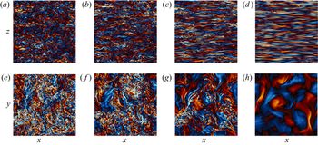
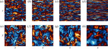
 $Fr_h$ from 0.0947 to 0.00935. Through the vertical slices in figures 6(a–d) and 7(a–d), we observe the transition in regimes from nearly isotropic small and intermediate scales to horizontally layered flow in the vorticity and temperature fluctuation fields. Obvious layers are not visible in the vorticity field at the weakest stratification
 $Fr_f=0.46$; the vertical temperature field slice in figure 7(a) better shows the slight anisotropy at
 $\textit {Re}_b=28.7$. At intermediate stratifications
 $Fr_f= 0.23$ and 0.12, KH instabilities are visible within recognizable horizontal layers in both the vorticity and temperature fields. Decreasing
 $Fr_f$ reduces the thickness of these layers, corresponding to an increase in
 $k_b$. The turbulence becomes increasingly patchy with increasing stratification and the corresponding decrease in
 $\textit {Re}_b$, with small-scale turbulence and overturning increasingly restricted to intermittent patches surrounded by viscously coupled layers (as in e.g. Brethouwer et al. Reference Brethouwer, Billant, Lindborg and Chomaz2007; Bartello & Tobias Reference Bartello and Tobias2013; Waite Reference Waite2014). For the strongest stratification
 $Fr_f=0.058$, overturning is restricted to very small vertical scales and only a few instabilities are visible in figures 6(d) and 7(d).
(a–d) Vertical slices  $(x,z)$ at
 $y=0$ of
 $y$-component vorticity. (e–h) Horizontal slices
 $(x,y)$ at
 $z=0$ of
 $z$-component vorticity.
 $\textit {Pr}=1$ for (a,e)
 $Fr_f=0.46$, (b,f)
 $Fr_f=0.23$, (c,g)
 $Fr_f=0.12$ and (d,h)
 $Fr_f=0.058$. The same colour map is used as in figure 3 with a modified range for visibility across
 $Fr_f$. The colour map range shared by the vertical slices is different from the range shared by the horizontal slices.

(a–d) Vertical slices  $(x,z)$ at
 $y=0$ of
 $\theta$. (e–h) Horizontal slices
 $(x,y)$ at
 $z=0$ of
 $\theta$.
 $\textit {Pr}=1$ for (a,e)
 $Fr_f=0.46$, (b,f)
 $Fr_f=0.23$, (c,g)
 $Fr_f=0.12$ and (d,h)
 $Fr_f=0.058$. The colour map range shared by the vertical slices is different from the range shared by the horizontal slices.

The horizontal slices in figures 6(e–h) and 7(e–h) show the loss of small scale features, as the small scales become less turbulent with smaller  $Fr_f$. This loss of small features can be attributed to
 $k_O$ growing from 15 to 297 between
 $Fr_f= 0.46$ and 0.058 while
 $k_d$ is only slightly increased. At larger
 $Fr_f$, the flow resembles small-scale isotropic turbulence for a wider wavenumber range
 $k\in [k_O,k_d]$, so the loss of small-scale features at
 $Fr_f=0.058$ is in line with greater anisotropy. At
 $Fr_f=0.058$, signatures of KH billows are still visible in the horizontal slices (figures 6h and 7h). These panels also exhibit the least extreme values in temperature and vorticity: as the horizontal layers are reduced to vertical scales near
 $k_d$ (and
 $k_B$ in the case of
 $\textit {Pr}=1$), fluctuations in these fields are eliminated by viscous dissipation and buoyancy diffusivity.
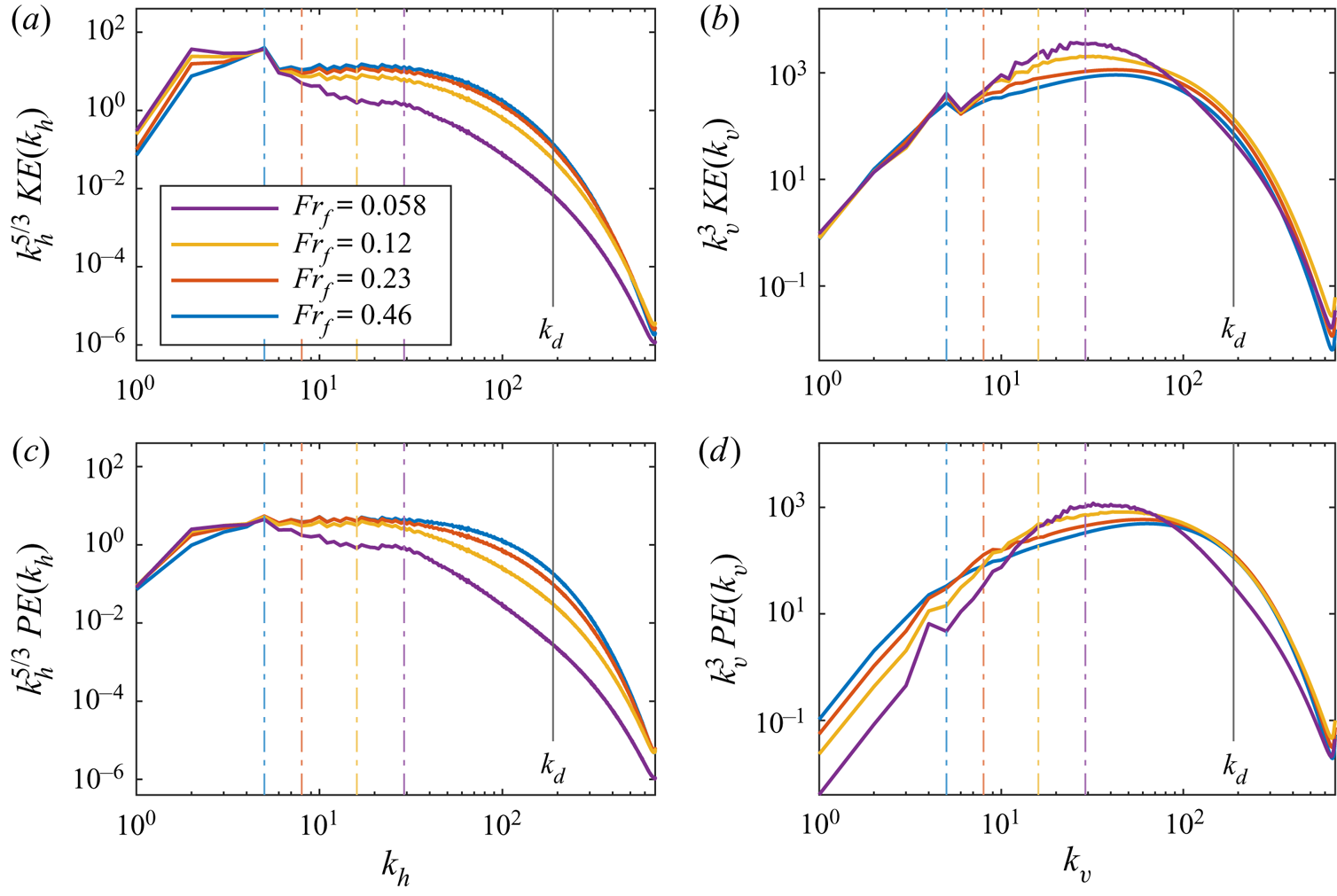
The compensated kinetic and potential energy spectra for  $\textit {Pr}=1$ at each
 $Fr_f$ are plotted in figure 8 in terms of horizontal and vertical wavenumber. For the horizontal kinetic energy spectra in figure 8(a), the
 $Fr_f= 0.46$, 0.23, and 0.12 cases are very similar. Slightly more kinetic energy is found at large scales for smaller
 $Fr_f$, and these cases show agreement with the
 $k_h^{-5/3}$ scaling law for almost a decade after the forcing interval. The vertical kinetic energy spectra in figure 8(b) are also affected by
 $Fr_f$. As
 $k_b$ increases with decreasing
 $Fr_f$, the compensated spectra approximately exhibit the +3 slope (as in § 3.1.1) for a longer range of small wavenumbers, but eventually converge at
 $k_v \approx 100$. A short plateau region corresponding to limited agreement with
 $k_v^{-3}$ scaling is observed at the three lowest stratifications.
Energy spectra in terms of horizontal and vertical wavenumbers for  $\textit {Pr}=1$ at different
 $Fr_f$. Vertical dash-dotted lines are buoyancy scales corresponding to
 $Fr_f$ colours. The average
 $k_d$ and
 $k_B$ are the same for
 $\textit {Pr}=1$.

The horizontal potential energy spectra for  $Fr_f= 0.46$, 0.23, and 0.12 follow the same patterns as the kinetic energy, but with marginally more
 $Fr_f$-dependence at intermediate and large
 $k_h$. Downscale of
 $k_b$, the spectra steepen more for smaller
 $Fr_f$ but eventually converge far into the dissipation range. More potential energy is found at intermediate to large
 $k_h$ at weaker stratification which is consistent with more small-scale overturning in the temperature field. The compensated vertical potential energy spectra nearly have the
 $+3$ slope up until their respective
 $k_b$, and exhibit similar dependence on
 $Fr_f$ as in the vertical kinetic energy spectra.
In all panels, the  $Fr_f=0.058$ spectra have a distinct shape compared to the three weaker stratifications. Since
 $\textit {Re}_b=0.6<1$, in this case, the cascade to small horizontal scales is suppressed and there is a consequent steepening of the horizontal spectra (e.g. Brethouwer et al. Reference Brethouwer, Billant, Lindborg and Chomaz2007; Waite Reference Waite2014). The steepening of the
 $Fr_f=0.058$ horizontal spectra at small wavenumbers is severe enough that there is little
 $k_h^{-5/3}$ scaling law agreement just downscale of the forcing. Similarly, the steepening from
 $k_b$ onwards causes the
 $Fr_f=0.058$ vertical spectra to deviate from
 $k_v^{-3}$ scaling. Except in figure 8(b), the
 $Fr_f=0.058$ case does not converge to the other three cases until the end of the wavenumber range. Strong stratification will restrict vertical advection, which greatly reduces the potential energy found at small vertical length scales.
3.2. The $\textit {Pr}$-dependence

3.2.1. Energy spectra
We now examine the effects of varying  $\textit {Pr}$ in fixed-
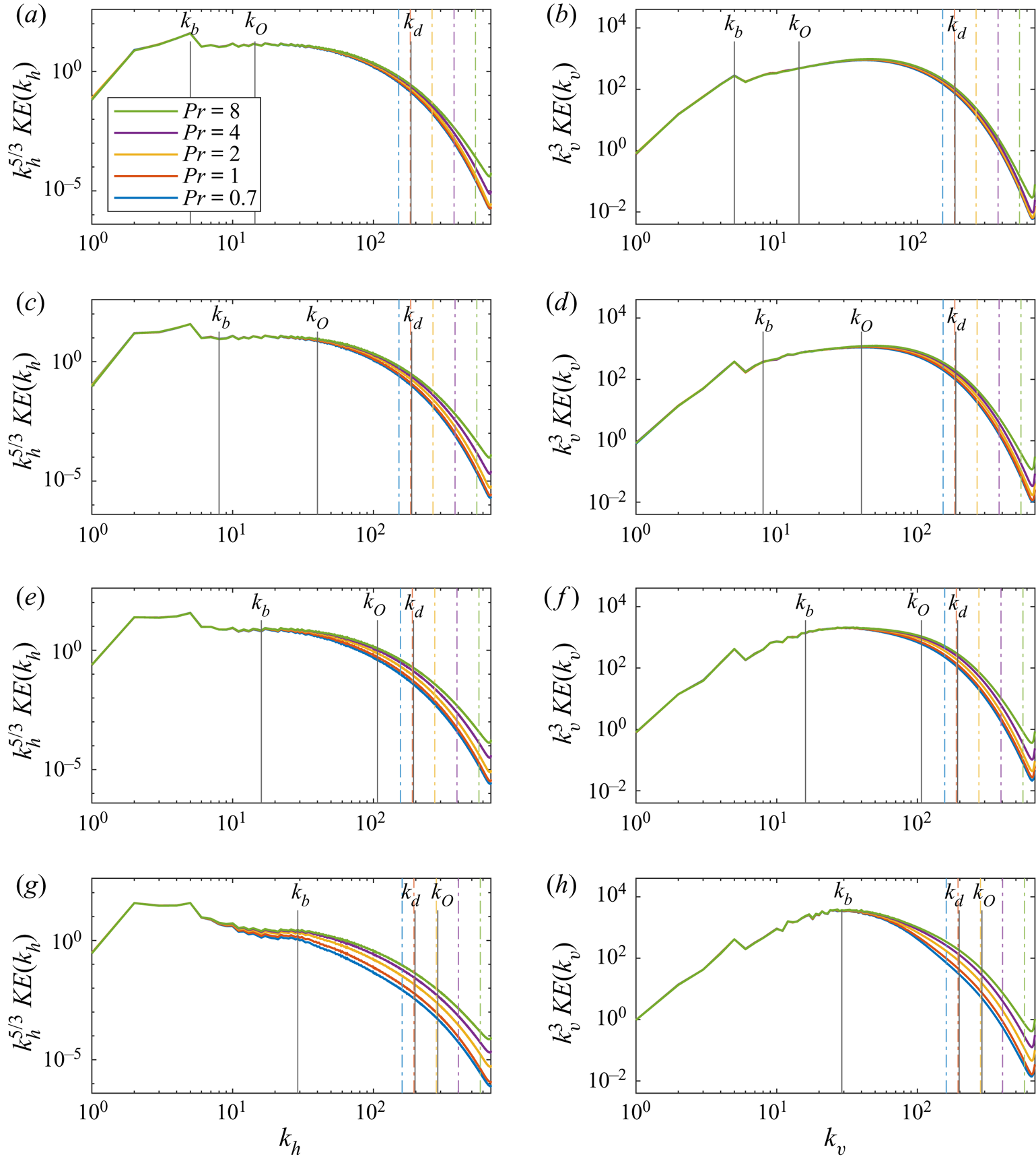
 $Fr_f$ groups, starting with the kinetic and potential energy spectra. The effect of
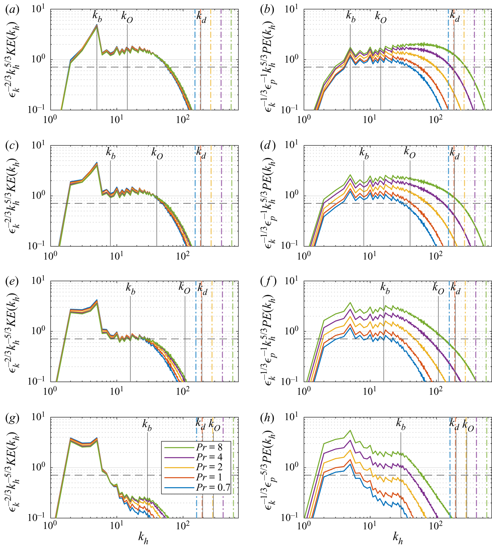
 $\textit {Pr}$ on the horizontal and vertical kinetic energy spectra, shown in figure 9, is more obvious and extends to larger scales as
 $Fr_f$ and
 $\textit {Re}_b$ decrease. Specifically, while
 $\textit {Pr}$-dependence for
 $Fr_f=0.46$ and 0.23 are mostly downscale of
 $k_O$ and around
 $k_d$ (figure 9a–d), the
 $Fr_h=0.12$ and 0.058 cases show
 $\textit {Pr}$-dependence that extends upscale past
 $k_O$ and into intermediate scales (figure 9e–h). Otherwise, as in figure 2, spikes at small wavenumbers are from the large-scale forcing, and the vertical spectra roughly have a
 $+3$ slope until
 $k_b$ regardless of
 $Fr_f$ and
 $\textit {Re}_b$. For
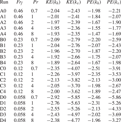
 $Fr_f = 0.46$, 0.23, and 0.12, the horizontal spectra follow the
 $k_h^{-5/3}$ scaling law just after the forcing interval for about one decade as in run C1 (see table 2). The
 $Fr_f=0.058$ spectra are steeper than those at larger
 $Fr_f$, with a more pronounced bump at
 $k_b$ (Waite Reference Waite2014). Similarly, in the vertical wavenumber spectra, a short plateau corresponding to the
 $k_v^{-3}$ scaling law is observed for almost one decade for all groups except
 $Fr_f=0.058$. Beyond these short scaling law intervals, both the horizontal and vertical spectra shallow slightly when
 $\textit {Pr}$ is increased (table 2). Larger-
 $\textit {Pr}$ simulations contain more kinetic energy at small scales since buoyancy-induced velocity fluctuations can persist as
 $k_B$ increases. As a result of the spectra shallowing, the
 $k_h^{-5/3}$ and
 $k_v^{-3}$ scaling laws extend to slightly smaller scales.
Compensated kinetic energy spectra in terms of horizontal and vertical wavenumbers for different  $\textit {Pr}$. From top to bottom the rows are
 $Fr_f= 0.46$, 0.23, 0.12, 0.058. Vertical dash-dotted lines are
 $k_B$ corresponding to
 $\textit {Pr}$ colours.

Slopes from linear regression analysis of kinetic and potential energy spectra in figures 9 and 10. For horizontal spectra, the linear regression is performed over  $k_h \in [6,60]$ except for
 $Fr_f=0.058$, where
 $k_h \in [6,29]$ is used. For vertical spectra, the wavenumber interval is one decade starting at
 $k_b$; i.e.
 $k_v \in [6,60],[8,80],[16,160]$ for
 $Fr_f=0.46,0.23,0.12$ respectively. The vertical spectra for
 $Fr_f=0.058$ uses
 $k_v\in [29,200]$ since the average
 $k_d \approx 198$.

As stratification increases, the dependence on  $\textit {Pr}$ extends to smaller wavenumbers. For example, the compensated horizontal kinetic energy spectra for different
 $\textit {Pr}$ start to diverge at
 $k_h \approx 30$ (between the Ozmidov and Kolmogorov wavenumbers) for
 $Fr_f=0.46$ and
 $k_h \approx 20$ (well upscale of the Ozmidov scale) for
 $Fr_f=0.12$ in figures 9(a) and 9(e) respectively. Only for the horizontal spectra with
 $Fr_f=0.058$ and
 $\textit {Re}_b < 1$ (figure 9g) do the spectra for each
 $\textit {Pr}$ separate shortly after the forcing interval, and at a wavenumber smaller than
 $k_b$.
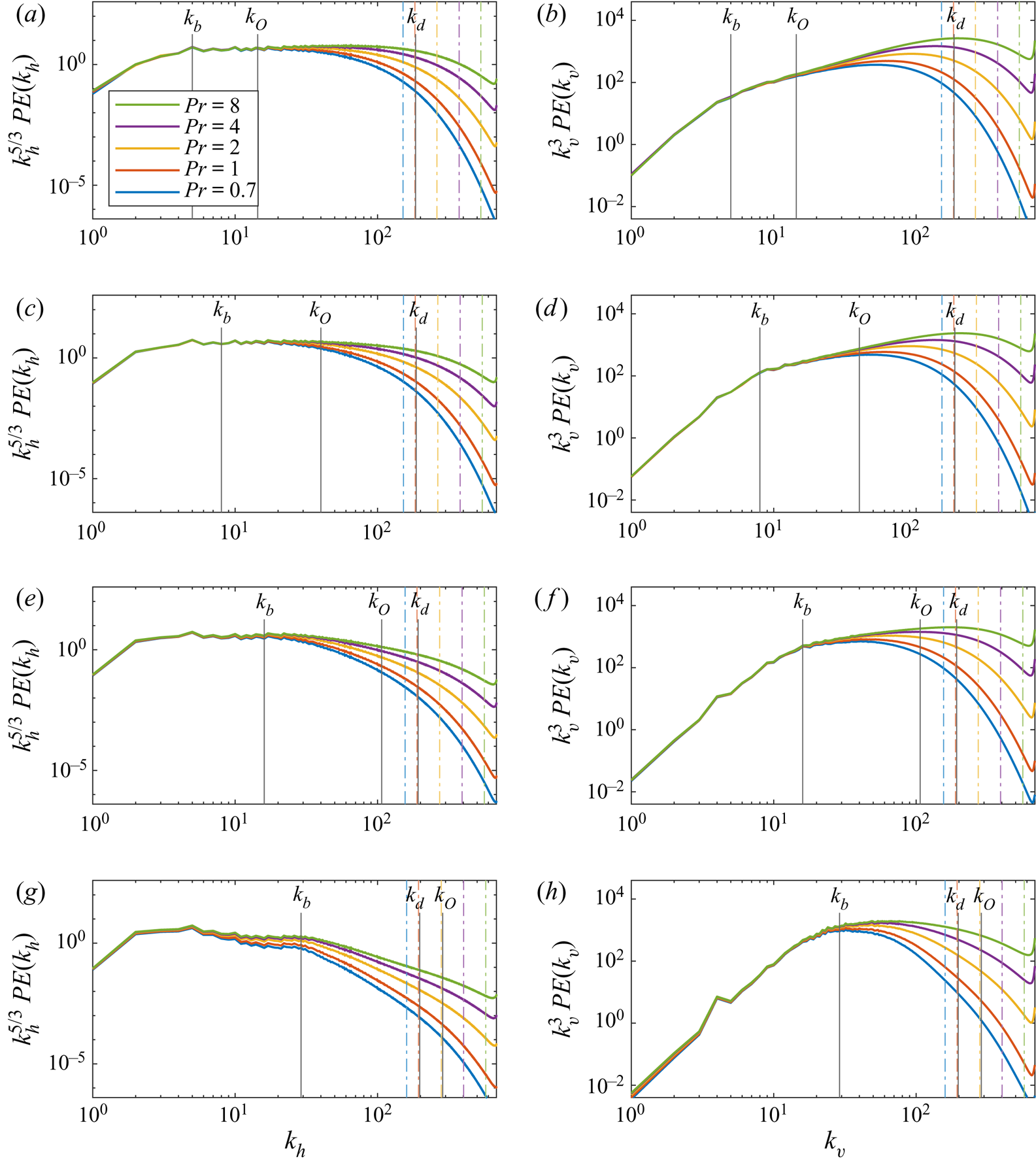
The potential energy spectra in figure 10 show similar but more pronounced changes as  $\textit {Pr}$ is varied. Both horizontal and vertical spectra exhibit the same shallowing with increased
 $\textit {Pr}$ at large wavenumbers as in the kinetic energy spectra (table 2). In the horizontal spectra, the shallowing that results from increasing
 $\textit {Pr}$ again lengthens the wavenumber range for which there is agreement with
 $k_h^{-5/3}$ scaling. Decreasing
 $Fr_f$ increases the average
 $k_b$, where a break in the vertical spectra is observed: immediately after
 $k_b$, the spectral slopes decrease toward a
 $k_v^{-3}$ scaling region. In the vertical spectra for
 $Fr_f= 0.46$, 0.23, and 0.12, the shallowing from larger
 $\textit {Pr}$ causes the spectra to become shallower than the
 $k_v^{-3}$ scaling law downscale of
 $k_b$.
Compensated potential energy spectra in terms of horizontal and vertical wavenumbers for different  $\textit {Pr}$. From top to bottom the rows are
 $Fr_f= 0.46$, 0.23, 0.12, 0.058. Vertical dash-dotted lines are
 $k_B$ corresponding to
 $\textit {Pr}$ colours.

The  $Fr_f=0.058$ potential energy spectra (figure 10g,h) behave similarly to the kinetic energy spectra at this stratification: here, both the horizontal and vertical spectra visibly separate just after the forcing interval and before
 $k_b$. The separation occurs at a noticeably smaller wavenumber for the horizontal spectra than the vertical, as in the kinetic energy case. All simulations with
 $Fr_f=0.058$ have
 $\textit {Re}_b<1$; horizontal scales between the forcing interval and the buoyancy scale are sensitive to
 $\textit {Pr}$ because of diffusive effects between the layers of quasi-horizontal vortices. Figure 10(g) for
 $Fr_f=0.058$ also shows a break in the horizontal spectra at
 $k_b$, after which each curve steepens beyond
 $k_h^{-5/3}$.
The Kolmogorov and Obukhov–Corrsin constants from (1.15) and (1.16) can be determined for each simulation from the fully compensated energy spectra,  $\epsilon _k^{-2/3} k_h^{5/3} E_K(k_h)$ and
 $\epsilon _k^{1/3} \epsilon _p^{-1} k_h^{5/3} E_P(k_h)$ (figure 11). Since the simulations in this work use the two-dimensional horizontal wavenumber
 $k_h$, the converted
 $C' \approx 1.40C$ values will be discussed. The compensated spectra generally show
 $C'_1$ and
 $C'_2$ to be larger than the value
 $C'=0.71$, corresponding to
 $C=0.51$ referenced in Lindborg (Reference Lindborg2006) and Brethouwer et al. (Reference Brethouwer, Billant, Lindborg and Chomaz2007). The kinetic energy spectra in the left column show
 $C'_1$ to be insensitive to
 $\textit {Pr}$ when
 $\textit {Re}_b > 1$. However, as
 $\textit {Re}_b$ increases and stratification decreases, the value of
 $C'_1$ tends to increase, which is consistent with the results of Brethouwer et al. (Reference Brethouwer, Billant, Lindborg and Chomaz2007), Bartello & Tobias (Reference Bartello and Tobias2013) (compared to figure 12 and figure 9(a) therein, respectively). Further, the present simulations with
 $\textit {Re}_b \approx 8$ (figure 11c) show
 $C'_1$ slightly larger than 0.71, similar to comparable simulations in Brethouwer et al. (Reference Brethouwer, Billant, Lindborg and Chomaz2007) (figure 13(a) therein,
 $\textit {Re}_b\approx 9$) and Bartello & Tobias (Reference Bartello and Tobias2013) (figure 9(a) therein, cyan curve,
 $\textit {Re}_b \approx 10$). The compensated potential energy spectra show
 $C'_2$ to be increasingly dependent on
 $\textit {Pr}$ as stratification increases and
 $\textit {Re}_b$ decreases. This may be attributed to the
 $\textit {Pr}$-dependence of the mixing efficiency: across all simulations, the sum
 $\epsilon _k + \epsilon _p$ is nearly held fixed, while the ratio
 $\epsilon _p/\epsilon _k$ decreases with larger
 $\textit {Pr}$. The potential energy spectra compensated with wavenumber only (figure 10, left column) are much less dependent on
 $\textit {Pr}$ when
 $\textit {Re}_b > 1$. The larger-
 $\textit {Pr}$ simulations simultaneously exhibit increasing
 $\epsilon _k$ and decreasing
 $\epsilon _p$, thereby resulting in
 $C'_2$ being strongly dependent on
 $\textit {Pr}$ through the premultiplication factor
 $\epsilon _k^{1/3} \epsilon _p^{-1}$.
Compensated horizontal wavenumber spectra for dimensional kinetic energy (a,c,e,g) and potential energy (b,d,f,h). From top to bottom the rows are  $Fr_f= 0.46$, 0.23, 0.12, and 0.058. Vertical dash-dotted lines are
 $k_B$ corresponding to
 $\textit {Pr}$ colours. Horizontal dashed lines are reference Kolmogorov and Obukhov–Corrsin constants of the two-dimensional horizontal spectra:
 $C'_1 = C'_2 = 0.71$ (Lindborg Reference Lindborg2006; Brethouwer et al. Reference Brethouwer, Billant, Lindborg and Chomaz2007).

For each increase in  $\textit {Pr}$, there appears to be less of a change in the shape of the spectra, and this behaviour is observed at all
 $Fr_f$. Excluding
 $\textit {Pr}=0.7$, each jump in
 $\textit {Pr}$ is from doubling the previous
 $\textit {Pr}$, but the shallowing or separation between successive curves slightly decreases, as evident in table 2. This is especially true at scales around and above the Kolmogorov scale. For instance, at the average
 $k_d=193$ for
 $Fr_f=0.12$, between
 $\textit {Pr}=1$ and
 $\textit {Pr}=2$ the horizontal kinetic energy increases by 67 % compared to a 38 % increase from
 $\textit {Pr} =4$ to
 $\textit {Pr} =8$. The vertical potential energy for the same
 $Fr_f$ and
 $k_d$ increases by 310 % between
 $\textit {Pr} =1$ and
 $\textit {Pr}=2$ compared to a 76 % increase from
 $\textit {Pr} =4$ to
 $\textit {Pr} =8$. Simulations where
 $\textit {Pr}$ is much greater than 8 may be expected to continue exhibiting less of a change in the potential energy spectrum shape as
 $\textit {Pr}$ is increased. That is, the diminishing increase and shallowing of spectra at larger
 $\textit {Pr}$ may become so inappreciable that these higher-
 $\textit {Pr}$ spectra converge to a shape not vastly different from the
 $\textit {Pr}=8$ case, at least at wavenumbers at and below
 $k_d$. At larger wavenumbers, for very large
 $\textit {Pr} \sim {O}(10^3)$, buoyant scalars have been shown to behave as passive scalars (i.e. potential energy spectra proportional to
 $k^{-1}$), and plateaus (
 $\propto k^0$) eventually develop in the potential energy spectra (Okino & Hanazaki Reference Okino, Hanazaki, Resch, Bez, Focht, Gienger and Kobayashi2017, Reference Okino and Hanazaki2019, Reference Okino and Hanazaki2020).
3.2.2. Buoyancy flux
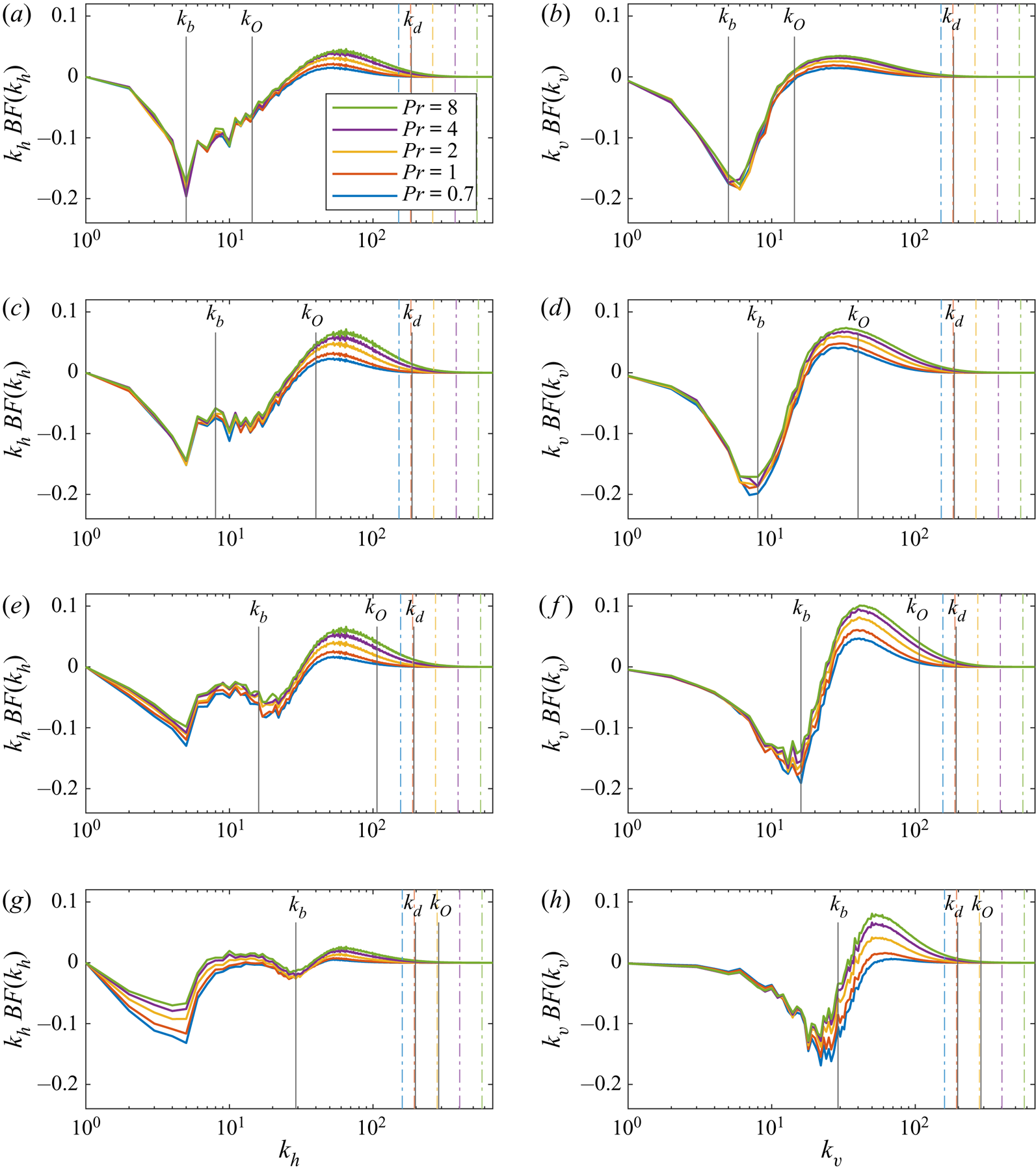
Buoyancy flux spectra are shown in figure 12 at different  $\textit {Pr}$ in fixed-
 $Fr_f$ groups as in § 3.2.1 for the energy spectra. Overall, an increase in buoyancy flux is observed in all cases as
 $\textit {Pr}$ is increased. The increase in buoyancy flux is most significant at large horizontal and vertical wavenumbers, where restratification occurs, and is amplified at smaller
 $Fr_f$. This increase in small-scale buoyancy flux with increasing
 $\textit {Pr}$ is consistent with the monotonic decrease in
 $\epsilon _p/\epsilon _k$, shown in table 1 and found in previous DNS studies of stratified turbulence (Smyth et al. Reference Smyth, Moum and Caldwell2001; Stretch et al. Reference Stretch, Rottman, Venayagamoorthy, Nomura and Rehmann2010; Salehipour et al. Reference Salehipour, Peltier and Mashayek2015); while the overall buoyancy flux is negative, an increase in small-scale buoyancy flux means that some small-scale potential energy is converted back to, and dissipated as, kinetic energy. The one exception to this trend is for the strongest stratification and smallest
 $\textit {Re}_b$ (figure 12g), where the increased buoyancy flux is greatest at small horizontal and large vertical wavenumbers. Additionally, at
 $Fr_f=0.058$, the horizontal buoyancy flux is positive for a short wavenumber range before
 $k_b$, as well as at larger wavenumbers, for
 $\textit {Pr}= 2$, 4 and 8. It makes sense that a greater amount of potential energy is converted to kinetic energy as
 $\textit {Pr}$ is increased: there is more potential energy available at large wavenumbers for either nonlinear transfer or conversion to kinetic energy when buoyancy diffusivity is weakened (figure 10). Restratification is less suppressed for less intense turbulence (Holloway Reference Holloway1988); indeed, for these simulations, increasing
 $\textit {Pr}$ at a fixed
 $Fr_f$ is associated with a decrease in
 $\textit {Re}$.
Buoyancy flux spectra multiplied by wavenumber to preserve area under the curve for linear–log axes. From top to bottom the rows are  $Fr_f= 0.46$, 0.23, 0.12 and 0.058. Horizontal (a,c,e,g) and vertical (b,d,f,h) wavenumber spectra are shown. Vertical dash-dotted lines are
 $k_B$ corresponding to
 $\textit {Pr}$ colours.

The right column of figure 12 shows restratification to consistently take place at small vertical scales downscale of  $k_b$. Due to the tendency towards isotropy at small scales, this positive spectral bump is also observed in the horizontal buoyancy flux spectra at a comparable
 $k_h$ range, at least for
 $Fr_f= 0.46$, 0.23 and 0.12. The
 $Fr_f=0.058$ case is different. All these simulations have
 $\textit {Re}_b<1$; as a result, there is no small-scale isotropy, and these small vertical scales are associated with large horizontal scales by viscously coupled layers. In this regime of stratified turbulence, it is reasonable that the buoyancy flux at large horizontal scales is heavily affected by
 $\textit {Pr}$, since buoyancy diffusion at small vertical scales can characteristically occur between these layers. Figure 12(g) also reveals that the
 $\textit {Pr}$-dependence of buoyancy flux is sensitive enough at large horizontal scales to even influence the direction of kinetic-to-potential energy conversion. Buoyancy diffusion can become weak enough at a sufficiently large
 $\textit {Pr}$ so that at large horizontal scales, enough surplus potential energy may be made available for a positive buoyancy flux.
The dependence on  $\textit {Pr}$ seems to be decreasing with increasing
 $\textit {Pr}$, as seen in the energy spectra. For example, the separation between the buoyancy flux spectra in the
 $\textit {Pr}=4$ and
 $\textit {Pr}=8$ cases is noticeably smaller than for preceding
 $\textit {Pr}$ increments. This suggests convergence of the buoyancy flux spectra at large
 $\textit {Pr}$ (even more so than for the energy spectra).
3.2.3. Spectral flux
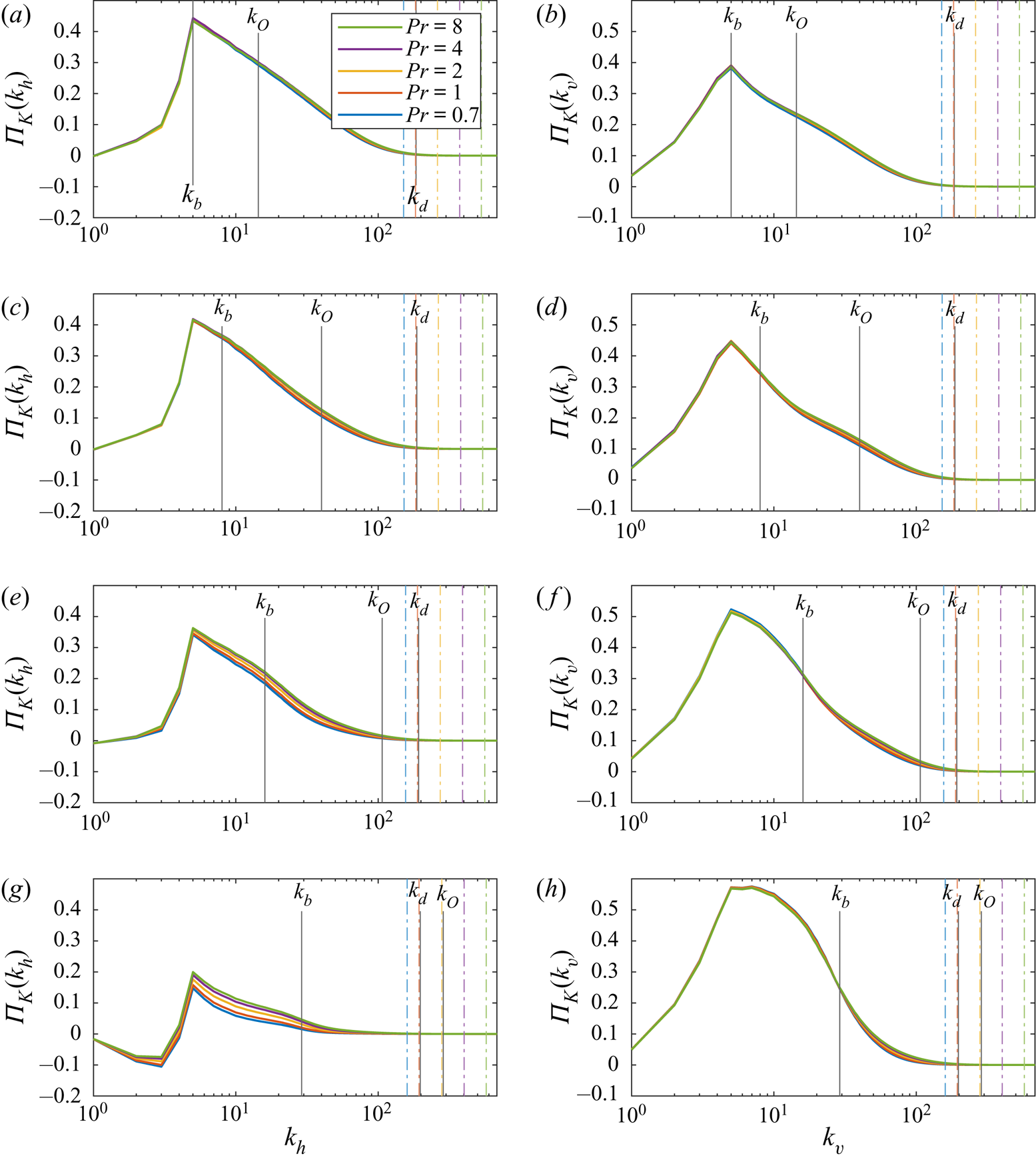
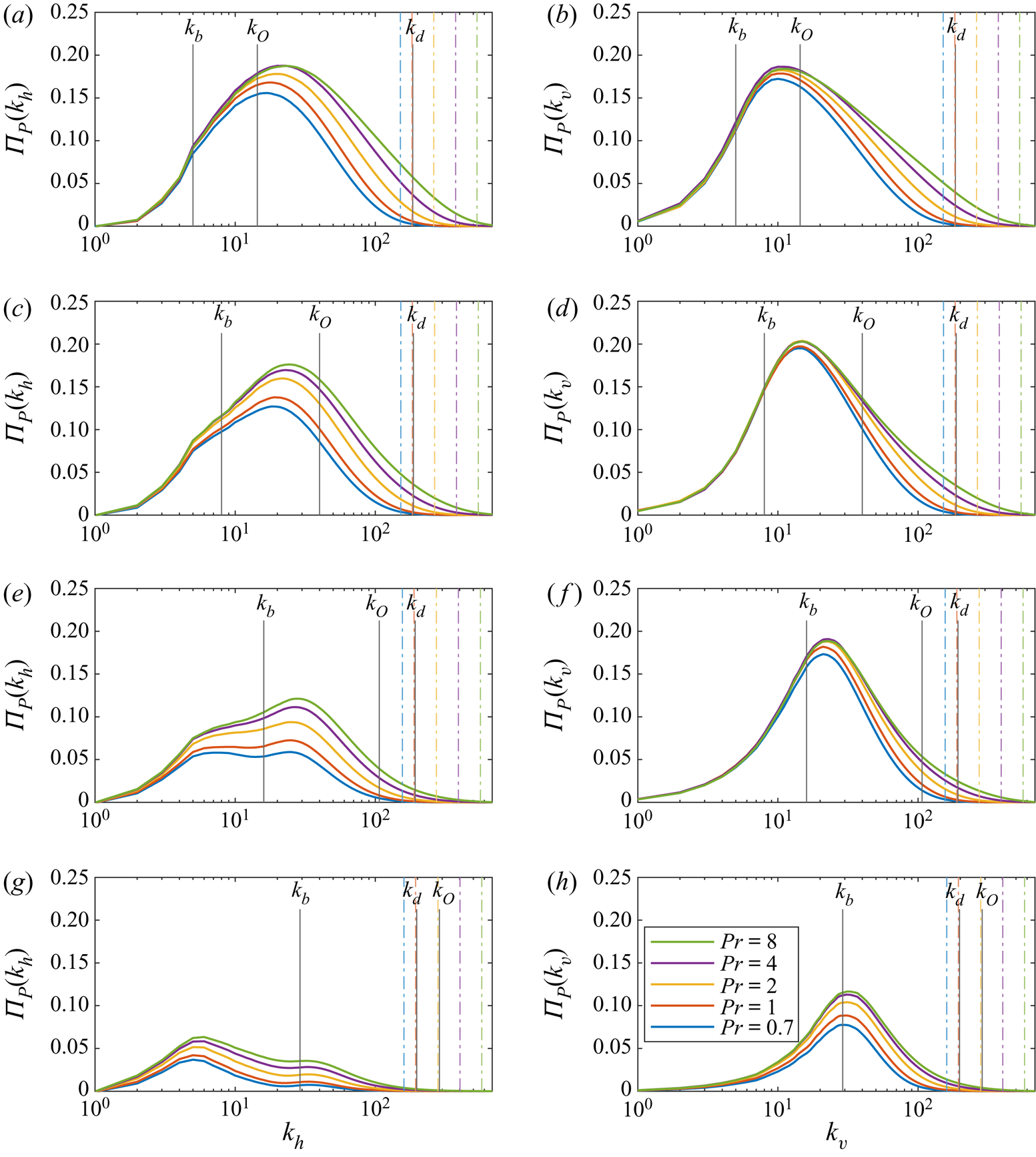
The spectral energy fluxes  $\varPi _K$ and
 $\varPi _P$ are shown in figures 13 and 14, respectively. The spectral flux for kinetic energy is not significantly affected by varying
 $\textit {Pr}$, especially for the vertical wavenumber spectra (figure 13b,d,f,h). For the intermediate stratifications
 $Fr_f = 0.23$ and 0.12, while there is a slight increase in flux with increasing
 $\textit {Pr}$, the fluxes at each
 $\textit {Pr}$ are scarcely distinguishable between the forcing interval and dissipation range in both horizontal and vertical spectra.
Spectral kinetic energy flux, as in (2.12). From top to bottom the rows are  $Fr_f= 0.46$, 0.23, 0.12 and 0.058. Horizontal (a,c,e,g) and vertical (b,d,f,h) wavenumber spectra are shown. Vertical dash-dotted lines are
 $k_B$ corresponding to
 $\textit {Pr}$ colours.

Spectral potential energy flux, as in (2.13). From top to bottom the rows are  $Fr_f= 0.46$, 0.23, 0.12 and 0.058. Horizontal (a,c,e,g) and vertical (b,d,f,h) wavenumber spectra are shown. Vertical dash-dotted lines are
 $k_B$ corresponding to
 $\textit {Pr}$ colours.

The  $Fr_f=0.058$ case is different, and shows a greater dependence of
 $\varPi _K(k_h)$ and
 $\varPi _K(k_v)$ on
 $\textit {Pr}$. The horizontal flux
 $\varPi _K(k_h)$ changes with
 $\textit {Pr}$ at large horizontal scales (figure 13), and is the only case where the fluxes are negative for a short wavenumber range. At very small horizontal wavenumbers, upscale transfer and accumulation of energy at large scales would appear as positive
 $T_K(k_h)$ at small
 $k_h$, corresponding to the energy contained in vertically sheared horizontal layers when
 $\textit {Re}_b<1$. Downscale of the forcing interval, the
 $\textit {Pr}$-dependence of
 $\varPi _K(k_h)$, while more apparent than at lower stratifications, is still minor. From the buoyancy flux in figure 12(g), less kinetic energy is lost by conversion to potential energy at greater
 $\textit {Pr}$, slightly increasing the available kinetic energy for downscale transfer. The vertical flux
 $\varPi _K(k_v)$ for
 $Fr_f=0.058$ is the closest to displaying a (short) constant flux range. Otherwise, varying
 $\textit {Pr}$ has little effect on
 $\varPi _K(k_v)$.
The impact of  $\textit {Pr}$ on the potential energy spectral flux is more pronounced than for the kinetic flux (figure 14). In all cases, increasing
 $\textit {Pr}$ increases the potential energy spectral flux. From figure 10, an increase in potential energy is found with larger
 $\textit {Pr}$, but for a limited wavenumber range. In the horizontal flux
 $\varPi _P(k_h)$ for cases
 $Fr_f=0.46$, 0.23 and 0.12, the most significant change is at intermediate-to-high wavenumbers, but the large horizontal scales are still minimally affected. The
 $Fr_f= 0.46$ case shows
 $\textit {Pr}$-dependence only for
 $k_h>k_b$, but for more strongly stratified cases, the
 $\textit {Pr}$-dependence extends up to the forcing interval. The termination of forward potential energy flux adjusts with
 $\textit {Pr}$ as expected, and more potential energy is made accessible for downscale transfer at large horizontal scales, since buoyancy diffusion acts on a shorter range of associated vertical scales.
The vertical spectral fluxes are almost unaffected by  $\textit {Pr}$ upscale of
 $k_b$ in all but the most strongly stratified case. This is to be expected of stratified turbulence, as the buoyancy scale characterizes the horizontal layer thickness and largest vertical overturning scale; the processes responsible for potential energy transfer should be limited by
 $k_b$.
Both the horizontal and vertical potential energy fluxes are far smaller for  $Fr_f=0.058$ than the three weaker stratifications. Notably, for
 $Fr_f=0.58$, the influence of
 $\textit {Pr}$ on the horizontal and vertical spectra persist for almost the entire wavenumber range. In the vertical flux,
 $\textit {Pr}$-dependence of the potential energy flux even occurs at vertical scales larger than the layer thickness as the flow becomes more anisotropic with
 $\textit {Re}_b<1$. A change in
 $\varPi _P$ would be expected when buoyancy diffusivity is weakened, but the influence of
 $\textit {Pr}$ extends upscale past the dissipation range in figure 14. The potential energy spectral fluxes are closer to exhibiting ranges of constant flux than for kinetic energy, but
 $\textit {Re}$ may still be too small for a discernible inertial range.
Again, as in the buoyancy flux spectra and energy spectra, the difference in both spectral energy fluxes between  $\textit {Pr}=4$ and
 $\textit {Pr}=8$ is noticeably smaller than the preceding increases of
 $\textit {Pr}$. As
 $\textit {Pr}$ increases,
 $\varPi _K$ and
 $\varPi _K$ may also be expected to converge to limiting curves.
3.2.4. Physical space fields
Lastly, slices of physical space fields are examined for fixed  $Fr_f=0.12$ as
 $\textit {Pr}$ is increased (
 $\textit {Pr}=0.7$ is excluded as it is similar to the
 $\textit {Pr}=1$ case). Since they have fixed
 $Fr_f$, these runs have a similar
 $\textit {Re}_b \approx 2$; the only noticeable change in the velocity, vorticity, and temperature fluctuation fields is that smaller-scale features emerge as
 $\textit {Pr}$ increases. The changes are subtle, but close inspection of the
 $\theta$ field slices in figure 15 reveal the finer structures that are able to persist with larger
 $\textit {Pr}$. The patchiness of the turbulence, which varies strongly with
 $\textit {Re}_b$, does not seem to depend much on
 $\textit {Pr}$. This trend is also observed in the velocity and vorticity fields, so only the temperature and the potential energy dissipation field are shown in figures 15 and 16.
(a–d) Vertical slices  $(x,z)$ at
 $y=0$ of
 $\theta$. (e–h) Horizontal slices
 $(x,y)$ at
 $z=0$ of
 $\theta$. Fixed
 $Fr_f=0.12$ for (a,e)
 $\textit {Pr}=1$, (b,f)
 $\textit {Pr}=2$, (c,g)
 $\textit {Pr}=4$ and (d,h)
 $\textit {Pr}=8$. The same colour map is used as in figure 3 with the range modified for visibility across
 $\textit {Pr}$. The colour map range shared by the vertical slices is different from the range shared by the horizontal slices.

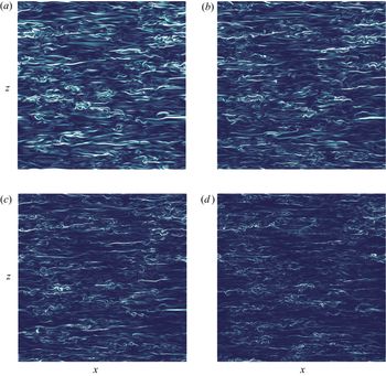
Vertical slices  $(x,z)$ at
 $y=0$ of
 $\epsilon _p$. Fixed
 $Fr_f=0.12$ for (a)
 $\textit {Pr} = 1$, (b)
 $\textit {Pr}=2$, (c)
 $\textit {Pr}=4$, (d)
 $\textit {Pr}=8$. The same colourmap is used for all panels as in figure 4(b), with the range modified for visibility across
 $\textit {Pr}$.

Vertical slices of the potential energy dissipation field are plotted in figure 16 for  $\textit {Pr}= 1$, 2, 4 and 8. The dissipative regions follow the horizontal layers, including the small-scale overturning and instabilities. At smaller
 $\textit {Pr}$, a bigger portion of the domain is dissipative, since a wider range of small scales is accessible to the stronger buoyancy diffusivity. The dissipative regions at
 $\textit {Pr}=8$ are limited to extremely fine scales, which is in agreement with the largest
 $k_B$ for
 $Fr_f=0.12$. Larger-
 $\textit {Pr}$ simulations are expected to exhibit even smaller-scale details in their physical fields, but may require higher resolution than
 $n=1536$ used here.
3.3. The $\textit {Re}_b$-dependence

To consider possible  $\textit {Pr}$-dependence at even higher
 $\textit {Re}_b$, simulations A1 and A4 were continued at higher resolution and Reynolds number for approximately 7 forcing time scales. These simulations have
 $\textit {Re}_b \approx 50$ at
 $Fr_f=0.46$, with half the original viscosity
 $\nu =0.06\ \textrm {cm}^2\,\textrm {s}^{-1}$ and increased resolution
 $n=1920$. These simulations are reported as A1h (
 $\textit {Pr}=1, Fr_f=0.46$) and A4h (
 $\textit {Pr}=8, Fr_f=0.46$) in table 1. As discussed in § 3.2.2 for the lower
 $\textit {Re}_b$ simulations, a decrease in
 $\epsilon _p/\epsilon _k$ as
 $\textit {Pr}$ increases from 1 to 8 is also found for
 $\textit {Re}_b \approx 50$. However, the drop in this ratio as
 $\textit {Pr}$ goes from 1 to 8 is less at
 $\textit {Re}_b \approx 50$ (24 %) than at
 $\textit {Re} _b \approx 30$ (39 %).
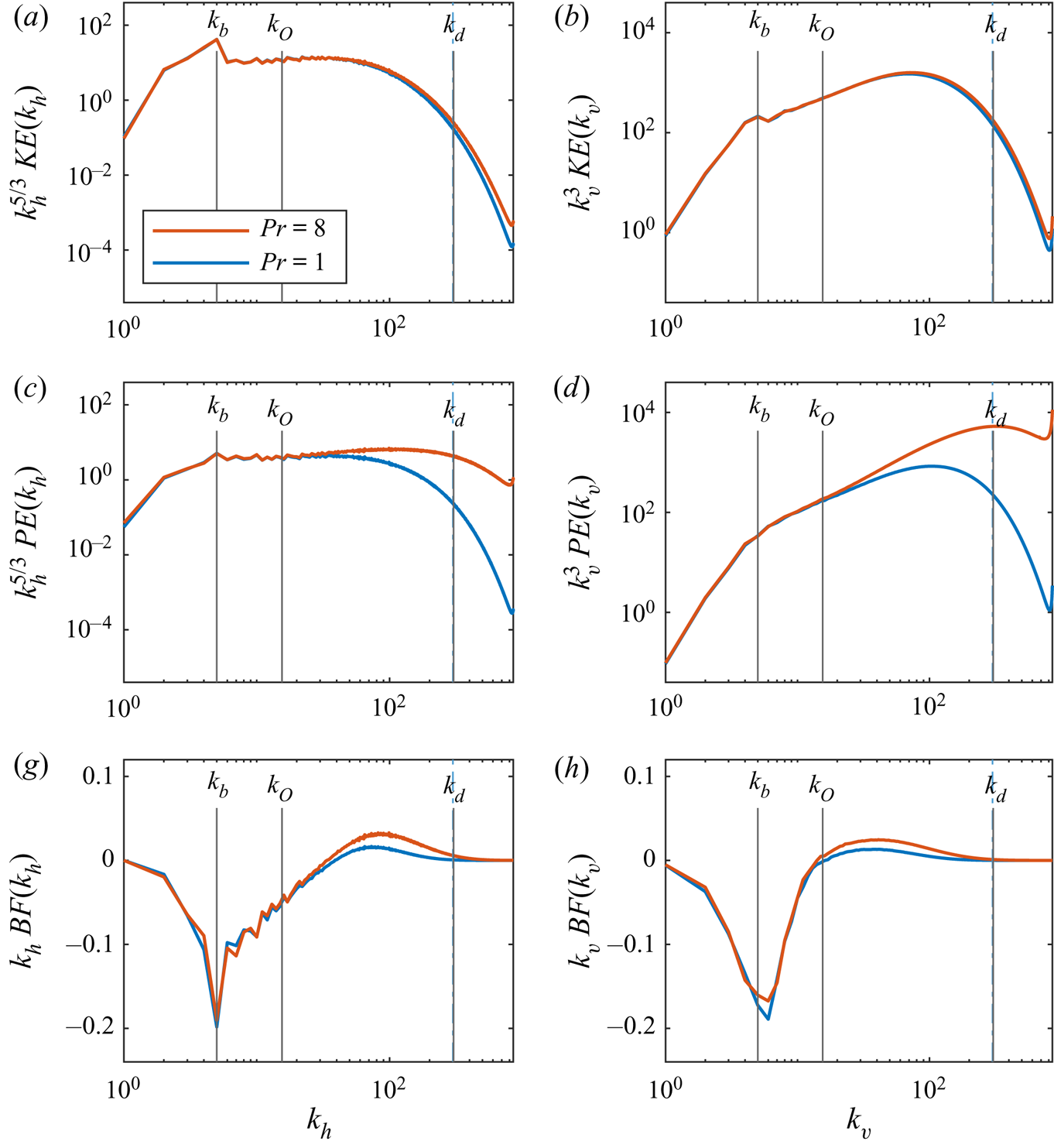
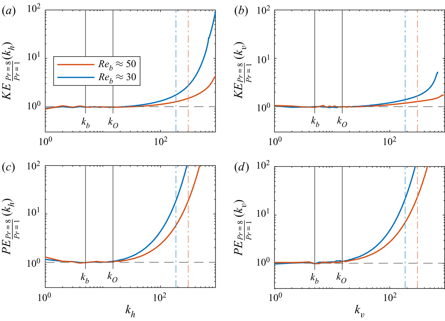
Energy and buoyancy flux spectra from the higher- $\textit {Re}_b$ simulations are plotted in figure 17. The spectra are mostly consistent with the previous sections’ results with respect to
 $\textit {Pr}$-dependence. Kinetic energy spectra in figure 17(a,b) are minimally affected by the increase in
 $\textit {Pr}$ from 1 to 8, even less than what was seen with
 $\textit {Re}_b \approx 30$ in figure 9(a). Potential energy spectra in figure 17(c,d) are far more sensitive than kinetic energy to
 $\textit {Pr}$ downscale of the Ozmidov scale and into the dissipation range. A longer plateau in the horizontal potential energy spectra, indicating a longer
 $k_h^{-5/3}$ scaling law range, is observed for
 $\textit {Pr}=8$ than for
 $\textit {Pr}=1$ past
 $k_b$ and into the
 $k_h \in [k_O, k_d]$ subrange, which has been slightly widened in response to the larger
 $\textit {Re}_b$. The buoyancy flux spectra show little influence from
 $\textit {Pr}$ outside of the restratification wavenumber ranges, as in the previous buoyancy flux plots in figure 12(a,b) at the same stratification,
 $Fr_f=0.46$. As above, this restratification leads to a decrease in the ratio
 $\epsilon _p/\epsilon _k$ as
 $\textit {Pr}$ increases from 1 to 8.
Compensated kinetic and potential energy spectra, and premultiplied buoyancy flux spectra for runs A1h ( $\textit {Pr}=1$) and A4h (
 $\textit {Pr}=8$). Horizontal (a,c,e) and vertical (b,d,f) wavenumber spectra are shown. Vertical dash-dotted lines are
 $k_B$ corresponding to
 $\textit {Pr}$ colours.

To compare the effect of  $\textit {Re}_b$ on the examined energy spectra, ratios of
 $\textit {Pr}=8$ spectra to
 $\textit {Pr}=1$ spectra are computed for
 $\textit {Re}_b \approx 30$ and
 $\textit {Re}_b \approx 50$ and plotted in figure 18. We find that the kinetic energy spectra at and above the Kolmogorov scale, and therefore also at and above the Ozmidov scale, are less sensitive to changes in
 $\textit {Pr}$ as
 $\textit {Re}_b$ increases. Even at large wavenumbers where the ratio increases from one, ratio values for
 $\textit {Re}_b \approx 30$ at a particular wavenumber are not realized in the
 $\textit {Re}_b \approx 50$ case until a wavenumber that is greater by at least 100. Indeed, the ratio at
 $k_d$ with
 $\textit {Re}_b \approx 50$ is smaller than the ratio at
 $k_d$ with
 $\textit {Re}_b \approx 30$, especially in the horizontal wavenumber spectrum. This finding suggests that the kinetic energy spectra at scales at and above the Kolmogorov scale are not very sensitive to
 $\textit {Pr}$ when
 $\textit {Re}_b \approx 50$. By contrast, potential energy is different: figure 18(c,d) show that potential energy spectra are insensitive to
 $\textit {Pr}$ around and above the Ozmidov scale, but they are much more sensitive to
 $\textit {Pr}$ than the kinetic energy spectra around the Kolmogorov scale (a common vertical axis scaling is used for all four panels). Indeed, the potential energy spectra ratios at the respective
 $k_d$ are approximately 10 for both values of
 $\textit {Re}_b$, and show no evidence of decreasing with increasing
 $\textit {Re}_b$.
Ratios of  $\textit {Pr}=8$ to
 $\textit {Pr}=1$ spectra for
 $\textit {Re}_b \approx 30$ (runs A1, A4) and
 $\textit {Re}_b \approx 50$ (runs A1h, A4h). Ratios of horizontal (a,c) and vertical (b,d) wavenumber spectra are shown. Vertical dash-dotted lines are
 $k_d$ corresponding to
 $\textit {Re}_b$ colours.

Overall, we can draw a few conclusions about the potential for  $\textit {Pr}$-independence of stratified turbulence spectra at different
 $\textit {Re}_b$. The potential energy is clearly the most sensitive to increases in
 $\textit {Pr}$ for all
 $\textit {Re}_b$. The main effect of increasing
 $\textit {Pr}$ is increased potential energy at small scales, and associated enhanced positive buoyancy flux and restratification as a consequence of the increased potential energy and vertical motion permitted by larger
 $\textit {Pr}$. Sensitivity to
 $\textit {Pr}$ is even observed upscale of the dissipative scales at all
 $\textit {Re}_b$ considered here. Much larger
 $\textit {Pr}$ may be needed to observe
 $\textit {Pr}$-independence in the potential energy around the Kolmogorov scale. The potential energy spectra at the Ozmidov scale, however, is far less sensitive to increases in
 $\textit {Pr}$ by
 $\textit {Pr}=8$, particularly for the larger values of
 $\textit {Re}_b \gtrsim 8$ (simulation groups A and B), i.e. for a wide scale separation between the Kolmogorov and Ozmidov scales. As this scale separation increases with increasing
 $\textit {Re}_b$,
 $\textit {Pr}$-independence in the potential energy could possibly be reached at the Ozmidov scale for even smaller
 $\textit {Pr}<8$ with larger
 $\textit {Re}_b$ than considered here. On the other hand, the kinetic energy spectra are independent of
 $\textit {Pr}$ at and upscale of the Kolmogorov scale for
 $\textit {Pr}$ as small as 8, and as long as
 $\textit {Re}_b>1$. When
 $\textit {Pr}$ is increased from 4 to 8, the increase in buoyancy flux seems to be overcome by viscous dissipation so that the kinetic energy at these scales does not change much. Therefore, using
 $\textit {Pr}=8$ seems adequate to simulate larger
 $\textit {Pr}$ flows with
 $\textit {Re}_b>1$ as long as the main focus is on kinetic energy. For larger
 $\textit {Re}_b \approx 30$,
 $\textit {Pr}=1$ is adequate as the kinetic energy spectra with
 $\textit {Pr}=1$ and
 $\textit {Pr}=8$ are very similar.
The buoyancy flux spectra with  $\textit {Re}_b \gtrsim 8$ also approach
 $\textit {Pr}$-independence by
 $\textit {Pr}=8$ at the Ozmidov scale. However, for the large values of
 $\textit {Re}_b \approx$ 30 and 50, the positive peak in buoyancy flux in the restratification range (which sees the most
 $\textit {Pr}$-sensitivity) occurs at scales smaller than the Ozmidov scale. As a result, the integrated buoyancy flux does not become independent of
 $\textit {Pr}$ for any
 $\textit {Re}_b$ considered here, which also suggests no
 $\textit {Pr}$-independence in the ratio
 $\epsilon _p/\epsilon _k$ or the mixing efficiency unless
 $\textit {Re}_b$ or
 $\textit {Pr}$ are even larger. For comparison, Okino & Hanazaki (Reference Okino and Hanazaki2020) show that the buoyancy flux spectra are nearly unchanged between the
 $\textit {Pr}=70$ and
 $\textit {Pr}=700$ cases, suggesting that
 $\textit {Pr}$-independence might be observed in the spectra for
 $\textit {Pr}$ as small as 70. Given that the decaying turbulence DNS in Okino & Hanazaki (Reference Okino and Hanazaki2019, Reference Okino and Hanazaki2020) have a small
 $\textit {Re}_b < 1$ for most of the integration time, it is possible that
 $\textit {Pr}$-independence of the buoyancy flux, and possibly also the mixing efficiency (or
 $\epsilon _p/\epsilon _k$), may be realized at a smaller
 $\textit {Pr}<70$ with larger
 $\textit {Re}_b$ where the separation between the Kolmogorov and Ozmidov scales is wider. Results from the present simulations show that the change in the related quantity
 $\epsilon _p/\epsilon _k$ from
 $\textit {Pr}=1$ to
 $\textit {Pr}=8$ decreases as
 $\textit {Re}_b$ increases, which relates to a similarly smaller change in the integrated buoyancy flux. Additional simulations with
 $\textit {Re}_b \gtrsim 30$ and larger
 $\textit {Pr}$ would be needed to reliably determine how buoyancy flux,
 $\epsilon _p/\epsilon _k$, and mixing efficiency is affected by
 $\textit {Re}_b$, a relationship that is possibly non-monotonic (Salehipour et al. Reference Salehipour, Peltier and Mashayek2015).
4. Conclusions
Direct numerical simulations of stratified turbulence were performed to study the effect of varying  $\textit {Pr}$ and to investigate the suitability for
 $\textit {Pr}=1$ simulations to reproduce
 $\textit {Pr} \neq 1$ results. The simulations presented here employed random forcing of large-scale vortical modes on cubic domains. A fixed viscosity and a set of
 $Fr_f$ were chosen to obtain a range of
 $\textit {Re}_b$ and
 $Fr_h$ as
 $\textit {Pr}$ was varied. Spectra of kinetic energy, potential energy, buoyancy flux, kinetic energy flux and potential energy flux were examined in fixed-
 $Fr_f$ groups to identify scale-specific results dependent on
 $\textit {Pr}$, and the effect of
 $\textit {Re}_b$ on
 $\textit {Pr}$-sensitivity was briefly examined. Snapshots of the velocity, vorticity, temperature fluctuation, and potential energy dissipation fields in physical space were also visualized for a qualitative analysis of
 $\textit {Pr}$-dependence.
When varying  $\textit {Pr}$, changes were naturally expected at very small scales, which is consistent with the change in
 $k_B$ (
 $k_d$ was nearly unchanged by
 $\textit {Pr}$ due to the fixed viscosity and forcing amplitude). Indeed, the most obvious
 $\textit {Pr}$-dependence in the kinetic and potential energy spectra was found at large wavenumbers, where the potential and kinetic energy grew with
 $\textit {Pr}$. The increase in energy can be explained by larger
 $\textit {Pr}$ permitting a wider wavenumber range of temperature fluctuations, possibly excited by enhanced inter-layer instabilities, which influence both kinetic and potential energy before viscous dissipation or buoyancy diffusion can occur. Since
 $k_d$ was not changed much by
 $\textit {Pr}$, the spectra of kinetic energy (and kinetic energy flux) were much less affected than potential energy (and potential energy flux). Subtle changes in the physical fields were found for different
 $\textit {Pr}$, except of course in the potential energy dissipation field (figure 16). This was not unexpected, as
 $\textit {Re}_b$ was only slightly changed for a fixed
 $Fr_f$, so no change to the transition between stratified turbulence regimes was incurred by varying
 $\textit {Pr}$.
The  $\textit {Pr}$-dependence was found upscale of the dissipation range in most of the examined spectra. In some cases, this even extended upscale into the large-scale forcing interval, particularly in the horizontal wavenumber spectrum. Intermediate-to-large-scale
 $\textit {Pr}$-dependence was visible more in the potential energy than kinetic energy spectra. The fully compensated energy spectra showed little
 $\textit {Pr}$-dependence of the Kolmogorov constant, while the Obukhov–Corrsin constant was highly dependent on
 $\textit {Pr}$, especially for stronger stratification. In the spectral kinetic energy flux, the
 $\textit {Pr}$-dependence was peculiar in that it only applied to
 $k_h$ and
 $k_v$ between the forcing interval and the dissipation range, where an inertial range could have existed if
 $\textit {Re}$ and/or
 $\textit {Re}_b$ were larger in these simulations. The spectral potential energy flux was extremely sensitive to
 $\textit {Pr}$ for most of the wavenumber range. The buoyancy flux spectra showed the strongest sensitivity to
 $\textit {Pr}$ in the restratification range just before
 $k_d$ and
 $k_B$, but also exhibited some
 $Fr_f$-dependence. Following the description by Holloway (Reference Holloway1988), it could be that for large
 $\textit {Pr}$, the increased abundance of potential energy at these small scales even further amplifies the conversion back to kinetic energy.
Among all the examined spectra, the most strongly stratified  $Fr_f=0.058$ cases were very different from the three weaker stratifications. The simulations with
 $Fr_f=0.058$ were the only cases in the
 $\textit {Re}_b<1$ regime; some of these observed differences may be consequences of the flow's transition to viscously coupled non-turbulent layers, as viscous and diffusive effects are expected when
 $\textit {Re}_b \lesssim 1$, even at large horizontal scales due to vertical viscous and diffusive effects of the viscously coupled layers. Breaks in the horizontal kinetic and potential energy spectra occurred at
 $k_b$ associated with the suppression of the downscale energy cascade in this regime. The horizontal buoyancy flux spectra in figure 12(g) showed that the forcing scales were most affected by
 $\textit {Pr}$, rather than the restratification range. In the spectral energy fluxes,
 $Fr_f=0.058$ was unique in that
 $\varPi _K(k_h)$ was affected by
 $\textit {Pr}$ only at intermediate-to-large scales, and both
 $\varPi _P(k_h)$ and
 $\varPi _P(k_v)$ showed
 $\textit {Pr}$-dependence for most of the wavenumber range. The
 $Fr_f=0.058$ cases also exhibited negative horizontal kinetic energy flux at large scales, implying an upscale transfer of energy when stratification is especially strong. None of the spectral fluxes displayed any discernible range of constant flux at any
 $Fr_f$ (except possibly
 $\varPi _K(k_v)$ at
 $Fr_f=0.058$). The development of a true inertial range may have been hindered by the small
 $\textit {Re}$ and especially
 $\textit {Re}_b$. The comparison between the
 $\textit {Re}_b \approx$ 30 and 50 simulations in § 3.3 (runs A1 and A4 versus runs A1h and A4h) show that at larger
 $\textit {Re}_b$, the kinetic energy spectra tend to be less sensitive to changes in
 $\textit {Pr}$, at least at scales around and above the Kolmogorov scale, which is reasonable given the weaker viscosity at
 $\textit {Re}_b \approx 50$.
Given the impact of  $\textit {Pr}$ upscale of the dissipation range, setting
 $\textit {Pr}=1$ to simulate realistic
 $\textit {Pr} > 1$ flows appears to be reasonable when
 $\textit {Re}_b \gtrsim 30$, when the focus is on kinetic energy at scales around and above the Kolmogorov scale. For smaller
 $\textit {Re}_b$, at smaller scales, and for other quantities involving potential energy,
 $\textit {Pr}=1$ is not a suitable choice. Depending on
 $Fr_f$,
 $\textit {Pr}$ was shown to affect the examined spectra with varied severity and at unexpected scales. In particular, the spectral potential energy flux was especially sensitive to
 $\textit {Pr}$, and was affected over more of its wavenumber range. For any investigation that might be reliant on accurately measured potential energy transfer, special care should be taken by properly computing these quantities using the appropriate
 $\textit {Pr}$ if possible. In addition, the ratio of potential to kinetic energy dissipation seems to be quite sensitive to
 $\textit {Pr}$, even for
 $\textit {Re}_b$ up to 50.
The exhibited shallowing of energy spectra with increasing  $\textit {Pr}$ was consistent with the results in Okino & Hanazaki (Reference Okino, Hanazaki, Resch, Bez, Focht, Gienger and Kobayashi2017, Reference Okino and Hanazaki2020). Further, in all the examined quantities it was suggested there could be convergence to a limiting spectrum shape as
 $\textit {Pr}$ increases, at least at scales around and above the Kolmogorov scale, as there was a declining growth in each spectrum with larger
 $\textit {Pr}$. That is, for
 $\textit {Pr}$ larger than 8 (but not extremely large as in Okino & Hanazaki Reference Okino, Hanazaki, Resch, Bez, Focht, Gienger and Kobayashi2017, Reference Okino and Hanazaki2020), and for large scales down to approximately
 $k_d$, it is expected that these examined spectra could converge to a shape not too different from the
 $\textit {Pr}=8$ case. Since varying
 $\textit {Pr}$ results in different
 $k_B$, it may only be at larger scales that convergence is possible. Okino & Hanazaki (Reference Okino and Hanazaki2019, Reference Okino and Hanazaki2020) also note less of a difference in spectra between different
 $\textit {Pr}$ as these
 $\textit {Pr}$ increase beyond 1;
 $\textit {Pr}$-independence could possibly be realized at some
 $\textit {Pr}<70$ in stratified turbulence for large
 $\textit {Re}_b$ (
 $\textit {Re}_b \approx 50$ is not quite large enough). The kinetic energy and spectral kinetic energy flux did not exhibit major dependence on
 $\textit {Pr}$, so performing DNS with
 $\textit {Pr}=1$ may be acceptable for those instances when large-scale kinetic energy is the main focus, as long as
 $\textit {Re}_b \gtrsim 30$. However, the potential energy, buoyancy flux, and spectral potential energy flux might not exhibit similarly close convergence until a much larger
 $\textit {Pr}>8$. Performing simulations with an accurate
 $\textit {Pr}$ may be crucial to reliably study these quantities.
Additional simulations with  $\textit {Pr}>8$ should be considered to further explore the extent of the predicted convergence in all of the observed spectra, but would demand a higher resolution than
 $n=1536$ used here. A wider range of
 $\textit {Re}_b$ as well as larger-
 $\textit {Re}$ simulations would allow for cases with identifiable inertial ranges to be studied. It may be of interest to explore any effects due to
 $\textit {Pr}$ on constant flux ranges, and to also see how restratification in the buoyancy flux spectra might change with more diverse cases. It would be very interesting to consider how results are (or are not)
 $\textit {Pr}$-dependent when
 $\textit {Re}_b \gtrsim O(100)$, however, the original challenge still remains: attainable values of
 $\textit {Pr}$,
 $\textit {Re}$, and
 $\textit {Re}_b$ will be limited by the available computational resources. For example, to perform a simulation with
 $\textit {Pr}=100$ with this set-up, it is estimated that a resolution of
 $n \approx 5000$ would be needed for
 $k_{max}/k_B=1$.
Future work on  $\textit {Pr}$-dependence of stratified turbulence could include the effects of rotation, which were neglected here. Based on the exhibited
 $\textit {Pr}$-dependence of the buoyancy flux, the effect of
 $\textit {Pr}$ on mixing efficiency may be an interesting extension of the work here. Exploring the very small scales and looking into possible changes in intermittency due to
 $\textit {Pr}$ is also of interest. Ultimately, the dependence of the small-scale instabilities that develop between layers on
 $Pr$, and the potential role of Holmboe in addition to KH instabilities (e.g. Peltier & Caulfield Reference Peltier and Caulfield2003; Salehipour, Caulfield & Peltier Reference Salehipour, Caulfield and Peltier2016), should be investigated. The forced simulations presented here were varied in a limited way (only
 $Fr_f$ and
 $\textit {Pr}$ were changed), but the code which produced them has many options to investigate stratified turbulence with different configurations. For example, one option could be to force fields other than the large vortical modes as shown here (e.g. velocity or temperature, possibly forcing large-scale gravity waves), or to modify some of the other forcing parameters.
Acknowledgements
This research was enabled in part by support provided by the Shared Hierarchical Academic Research Computing Network (SHARCNET), Compute/Calcul Canada, the Natural Sciences and Engineering Research Council of Canada (Grant No. RGPIN-386456-2015) and the Canadian Foundation for Innovation.
Declaration of interests
The authors report no conflict of interest.