1 Introduction
1.1 Nonlinear breaking waves
Nonlinear breaking waves are abundant in a wide range of natural as well as industrial processes involving two-phase air–water systems. On the surface of oceans, breaking waves are responsible for transferring energy from the atmosphere to the water bodies and directly affect turbulence and mixing in the oceans. Turbulent breaking waves also occur as a result of ship movement in the oceans. Nonlinear bow waves, boundary layer breaking waves and bores at the stern of ships are examples of such interactions. These waves act as an energy transfer mechanism from the ship to the water bodies, and they greatly impact the ships’ hydrodynamic performance. Other instances of wave breaking occur in rivers and canals. In addition to their role in turbulence generation and air entrainment, breaking waves are also responsible for scour, erosion and sediment transport in such systems (van Rijn Reference van Rijn1993; King Reference King1995). Despite the prevalence of nonlinear breaking waves, important aspects of their actions are not fully understood. Examples of such aspects include: turbulence generation and transport, turbulence interaction with the free surface, bubble generation and air entrainment.
The plunging event in a breaking wave typically entraps a large volume of air and simultaneously sets vorticity generation in the water. The interaction of entrapped air with turbulence causes the air mass to break into smaller bubbles, a process which increases the area of contact between air and water. The subsequent process of the dissolution of air into water is crucial for living organisms as well as for transferring greenhouse gases from the atmosphere to the ocean.
In recent years, air entrainment by free surface flows has received considerable attention in both experimental (Chanson Reference Chanson1996; Deane & Stokes Reference Deane and Stokes2002; Liu & Duncan Reference Liu and Duncan2003, Reference Liu and Duncan2006; Murzyn & Chanson Reference Murzyn and Chanson2009b ; Kiger & Duncan Reference Kiger and Duncan2012), and computational (Lubin et al. Reference Lubin, Vincent, Abadie and Caltagirone2006; Moraga et al. Reference Moraga, Carrica, Drew and Lahey2008; Lubin, Glockner & Chanson Reference Lubin, Glockner and Chanson2009; Lakehal & Liovic Reference Lakehal and Liovic2011; Ma et al. Reference Ma, Oberai, Lahey and Drew2011, Reference Ma, Oberai, Drew and Lahey2012) studies. In the context of breaking waves there are two types of regimes that can encounter air entrainment. The first regime involves transient waves, such as plunging breaking waves (Lamarre & Melville Reference Lamarre and Melville1991; Deane & Stokes Reference Deane and Stokes2002) and spilling breakers (Duncan et al. Reference Duncan, Qiao, Philomin and Wenz1999; Duncan Reference Duncan2001; Qiao & Duncan Reference Qiao and Duncan2001; Liu & Duncan Reference Liu and Duncan2003, Reference Liu and Duncan2006). The second regime involves statistically stationary waves, such as bores (Leng & Chanson Reference Leng and Chanson2015), bow waves (Dong, Katz & Huang Reference Dong, Katz and Huang1997; Wilson, Carrica & Stern Reference Wilson, Carrica and Stern2007) and boundary layer waves (Tahara & Stern Reference Tahara and Stern1996).
1.2 Hydraulic jump
Hydraulic jumps are a canonical form of nonlinear breaking waves in which bubbles are generated in a statistically stationary manner, while turbulence and the interface interact with each other. Investigations of turbulent hydraulic jumps date back decades (Rouse, Siao & Nagaratnam Reference Rouse, Siao and Nagaratnam1959). However, it is still an active topic of research (Wang, Murzyn & Chanson Reference Wang, Murzyn and Chanson2014). Rouse et al. (Reference Rouse, Siao and Nagaratnam1959) used a wind tunnel with a solid top wall to imitate the flow conditions of a hydraulic jump. Although their method did not involve relevant coupling with a free interface, it provided insight into the momentum and energy balance in such flows. Resch & Leutheusser (Reference Resch and Leutheusser1972) studied the turbulence intensities and Reynolds stresses in a stationary hydraulic jump with Froude numbers of 2.85 and 6, and noted the significant influence of the conditioning of the upstream flow (e.g. fully developed and not developed) on their measurements.
Madsen & Svendsen (Reference Madsen and Svendsen1983) developed a theoretical model for a velocity field and interface profile of stationary hydraulic jumps using a simplified
 $k$
–
 ${\it\varepsilon}$
model. Their model was successful in predicting the one-dimensional energy production and dissipation; however, the predictions of Reynolds stresses and interface height were less successful. Hornung, Willert & Turner (Reference Hornung, Willert and Turner1995) performed a control-volume analysis of a hydraulic jump in order to study the downstream mean vorticity as a function of Froude number. They compared their predictions of average vorticity with experimental results obtained by the digital particle image velocimetry (DPIV) technique on a hydraulic jump in translation and observed approximate agreement. They qualitatively explained the vorticity generation at the interface by a surface reconnection phenomenon occurring at the wave breaking.
Using high-speed photography, Long et al. (Reference Long, Rajaratnam, Steffler and Smy1991a
) studied the vorticity structure at the roller region of stationary hydraulic jumps and their interactions downstream. They quantified the length scales of roller vortices as a function of streamwise location, in Froude numbers ranging from 4 to 9. Later, Liu, Rajaratnam & Zhu (Reference Liu, Rajaratnam and Zhu2004), using micro acoustic Doppler velocimetry (MicroADV), studied the turbulence structures of stationary hydraulic jumps at low Froude numbers, and reported energy spectra of the velocity field. In a more recent study, Misra et al. (Reference Misra, Kirby, Brocchini, Veron, Thomas and Kambhamettu2008) studied the turbulence and mean flow structures in a weak stationary hydraulic jump with Froude number
 $1.19$
using a particle image velocimetry technique.
Rodriguez-Rodriguez et al. (Reference Rodriguez-Rodriguez, Marugan-Cruz, Aliseda and Lasheras2011) investigated the dynamics of steady breakers, using the bubble image velocimetry (BIV) technique. Their study focused on the dynamics of large eddies responsible for air entrainment. They reported similarities in flow features between steady breakers and turbulent shear layers. These similarities include the generation of an array of coherent vortices which convect downstream with a constant velocity, linear growth of the vortex size and self-similar profiles of mean velocity and Reynolds stresses. Among the differences they observed the vortices have larger convective velocity in shear layers, but faster growth of size with distance in steady breakers. In another study, Lin et al. (Reference Lin, Hsieh, Lin, Chang and Raikar2012) employed particle image velocimetry (PIV) and BIV to investigate stationary hydraulic jumps, and reported mean velocity profiles, turbulence intensity, Reynolds stresses and energy spectra. They established the usefulness of their BIV technique for the investigation of aerated regions of stationary hydraulic jumps. They also reported that the velocity spectra from bubbles follow a power law different from that for water.
1.3 Air entrainment by hydraulic jumps
In addition to turbulence production, hydraulic jumps also involve complex air entrainment processes. A series of investigations have focused on various aspects relating to air entrainment including the distribution of void fraction, bubble size distribution as well as interface statistics. Chanson (Reference Chanson1995) measured the air bubbles by a single-tip conductivity probe, and reported void fraction in stationary hydraulic jumps and plunging jets. Chanson & Brattberg (Reference Chanson and Brattberg2000) studied void fraction distribution, turbulence statistics and bubble frequency measurements for high Froude number flows, and reported significant aeration. Chanson (Reference Chanson2007a ) investigated the bubble clustering and void fraction distributions at high Froude numbers ranging from 4.6 to 8.6. Murzyn & Chanson (Reference Murzyn and Chanson2009a ) studied free surface fluctuations and free surface profiles for a similar range of Froude numbers. Current knowledge of air entrainment and flow characteristics in hydraulic jumps is summarized by Chanson (Reference Chanson2009).
In other studies, void fraction, bubble size and bubble frequencies at relatively low Froude numbers (
 $2<Fr<5$
) are investigated. Murzyn, Mouaze & Chaplin (Reference Murzyn, Mouaze and Chaplin2005) distinguished two regions with different void fraction properties in stationary hydraulic jumps. In the lower or shear region of the flow, they confirmed that the void fraction follows a Gaussian distribution, whereas in the upper region, which is dominated by free surface interactions, the void fraction follows an error function profile (Brattberg, Toombes & Chanson Reference Brattberg, Toombes and Chanson1998). Following the direction of this research, Murzyn, Mouaze & Chaplin (Reference Murzyn, Mouaze and Chaplin2007) investigated mean and turbulent flow fluctuations near the free surface, and quantified a measurable length scale associated with surface undulations. They observed that the position of maximum free surface fluctuations does not depend on Froude number; also, the interface length scales are independent of Froude and Weber numbers. Misra et al. (Reference Misra, Kirby, Brocchini, Veron, Thomas and Kambhamettu2008) studied the interface dynamics of a weak hydraulic jump, and defined the index of entrainment to be the coefficient of variation of the interface fluctuations. They showed that this index reaches its maximum at the breaking wave regions associated with the most intensive air entrainment.
1.4 Computational studies of hydraulic jumps
Despite the relatively large number of experimental investigations of breaking waves, numerical investigations on this subject are limited. Gharangik & Chaudhry (Reference Gharangik and Chaudhry1991) among others considered one-dimensional Boussinesq equations to describe the height and velocity change of a hydraulic jump on a slightly sloped bottom wall. Long, Steffler & Rajaratnam (Reference Long, Steffler and Rajaratnam1991b
) solved the two-dimensional Reynolds-averaged Navier–Stokes (RANS) equations with the
 $k$
–
 ${\it\varepsilon}$
turbulence model to describe the surface profile and mean velocities in hydraulic jumps. They employed ‘body fitted coordinates’ to describe only the water phase and fit their mesh to the water body. Chippada, Ramaswamy & Wheeler (Reference Chippada, Ramaswamy and Wheeler1994) employed a similar methodology, but with a moving body-fitted mesh to track the interface. Zhou & Stansby (Reference Zhou and Stansby1999) extended such calculations to the transverse direction, but solved only two-dimensional shallow water equations. Ma, Hou & Prinos (Reference Ma, Hou and Prinos2001) considered a two-dimensional
 $k$
–
 ${\it\varepsilon}$
model and an additional volume of fluid (VOF) equation to track the evolution of the free surface, and thus eliminated the need for use of complex body-fitted mesh algorithms. They used an earlier version of the VOF method which did not utilize the recent sharp surface reconstruction algorithms. Carvalho, Lemos & Ramos (Reference Carvalho, Lemos and Ramos2008) performed a similar RANS calculation, but with a VOF method that utilized geometric surface reconstruction. More recently, Lubin et al. (Reference Lubin, Glockner and Chanson2009) attempted to use VOF to perform LES of a two-dimensional (2-D) hydraulic jump without a RANS model. However, despite integrating the equations for a long physical time, they were not able to make the jump stable and stationary. Ma et al. (Reference Ma, Oberai, Lahey and Drew2011) simulated a 2-D RANS and a 3-D detached-eddy simulation (DES) hydraulic jump with a two-fluid model. They proposed an air entrainment model which was tuned based on the kinetic energy of the fluid and the mean velocity gradient near the interface. Their model involved multiple parameters that were tuned against experimental results such as the probability density function (PDF) of the bubble size distribution.
Given this overview, we should note that the high-fidelity details of turbulent hydraulic jumps are thus far dominantly provided by experimental investigations. Experimental measurements however, involve various challenges including lack of direct optical access to regions in which air and water are mixed near the interface, limitations on non-intrusive measurements of instantaneous 3-D velocity fields and limitations in resolution of field gradients. The latter two items are crucial for quantification of turbulent energy dissipation which plays a key role in governing the bubble size distribution (Hinze Reference Hinze1955; Li & Garrett Reference Li and Garrett1998; Garrett, Li & Farmer Reference Garrett, Li and Farmer2000; Deane & Stokes Reference Deane and Stokes2002).
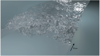
Calculation of a turbulent hydraulic jump with
 $Fr=2$
,
 $Re=11\,000$
and
 $We=1820$
.

1.5 Overview of the present investigation
The present work is the first high-fidelity simulation of a stationary turbulent hydraulic jump in which spatio-temporal scales associated with turbulence and the interface are resolved in three dimensions, as shown in figure 1. Our simulations resolve the Hinze scale and do not resort to any modelling to predict turbulence or air entrainment. In addition, our results provide the first direct measurement of turbulence dissipation and production in a turbulent breaking wave. Previous studies have shown a direct connection between turbulent dissipation and bubble size (Hinze Reference Hinze1955; Li & Garrett Reference Li and Garrett1998; Garrett et al. Reference Garrett, Li and Farmer2000; Deane & Stokes Reference Deane and Stokes2002) in the form of scaling laws. However, under realistic conditions, the dissipation field is not uniform, and thus different pieces of the entrained air can experience different dissipation intensities depending on their path in the flow. Still unclear is the degree to which the non-uniformity of the dissipation field plays a role in influencing the bubble size distribution. By providing spatially resolved turbulence dissipation fields, our DNS allows more intensive investigation of the processes determining bubble size distributions in breaking waves.
Our results also provide simultaneous measurements of flow statistics, such as mean velocity fields and Reynolds stresses, as well as air entrainment statistics for a breaking wave. This information provides crucial data for developing reduced-order models or new RANS models for air entrainment in breaking waves. Given the intimate coupling between turbulence equations and interface equations, it is crucial that such models be verified against data that simultaneously provide statistics of flow as well as air entrainment. Data from a hydraulic jump provide an excellent benchmark for such model developments since the hydraulic jump is the most canonical form of a turbulent breaking wave that can be fully characterized with a minimum number of parameters. Additionally, its statistical homogeneity in one spatial direction as well as in time allows for the collection of many ensembles and a meaningful reduction of statistics in lower-dimensional space. To this end, we provide data files containing statistics of the flow in the form of supplementary material, which is available at http://dx.doi.org/10.1017/jfm.2016.230.
Furthermore, we provide a 1-D (cross-section-averaged) accounting of various energy terms in the Navier–Stokes equations in the simulated hydraulic jump. In addition to providing insights about the nature and extent of the energy exchange processes downstream of the jump, these results can also be used for the development and verification of 1-D wave breaking models (Madsen & Svendsen Reference Madsen and Svendsen1983; Richard & Gavrilyuk Reference Richard and Gavrilyuk2013). The present simulations also shed new insight into coherent structures in turbulent hydraulic jumps and their dynamical role in air entrainment. Specifically, we have identified a vortex-shedding phenomenon through which spanwise vortices entrain air in the form of patches of bubbles as they are shed from the toe of the jump. Rodriguez-Rodriguez et al. (Reference Rodriguez-Rodriguez, Marugan-Cruz, Aliseda and Lasheras2011) reported air entrainment by vortex shedding from their experimental investigation of steady breakers. Our work confirms and quantifies these features in a hydraulic jump.
The paper is organized as follows: § 2 describes the mathematical formulation of the problem. Section 3 presents time-averaged statistics such as mean interface profile, mean velocities and fluctuations and Reynolds stresses. Section 4 presents a 1-D energy budget in the flow. Section 5 presents the turbulent dissipation field and estimation of the Hinze scale. In § 6 velocity spectra are presented. In § 7, air entrainment and its correlation with coherent vortex structures are introduced. We present the concluding remarks in § 8.
2 Problem set-up
2.1 Governing equations
The governing equations for incompressible two-phase flows are the continuity and balance of momentum,
 $$\begin{eqnarray}\displaystyle & \boldsymbol{{\rm\nabla}}\boldsymbol{\cdot }\boldsymbol{u}=0 & \displaystyle\end{eqnarray}$$
 $$\begin{eqnarray}\displaystyle & \displaystyle {\it\rho}\frac{\partial \boldsymbol{u}}{\partial t}+{\it\rho}\boldsymbol{u}\boldsymbol{\cdot }\boldsymbol{{\rm\nabla}}\boldsymbol{u}=-\boldsymbol{{\rm\nabla}}p+\boldsymbol{{\rm\nabla}}\boldsymbol{\cdot }({\it\mu}[\boldsymbol{{\rm\nabla}}\boldsymbol{u}+\boldsymbol{{\rm\nabla}}^{\text{T}}\boldsymbol{u}])+{\it\rho}\boldsymbol{g}+\boldsymbol{f}_{S}, & \displaystyle\end{eqnarray}$$
where
 $\boldsymbol{u}$
,
 $p$
,
 ${\it\rho},{\it\mu}$
,
 $\boldsymbol{g}$
and
 $\boldsymbol{f}_{S}$
are velocity, pressure, density, dynamic viscosity, gravitational acceleration and surface tension force, respectively. Equations (2.1) and (2.2) are defined in both air and water phases, while the surface tension force is active only at the interface. The surface tension force
 $\boldsymbol{f}_{S}$
is implemented with a sharp interface model using the Ghost Fluid Method technique (Fedkiw et al.
Reference Fedkiw, Aslam, Merriman and Osher1999), with an interface jump condition of
 $$\begin{eqnarray}[p]_{{\it\Gamma}}={\it\sigma}{\it\kappa}+[{\it\mu}]_{{\it\Gamma}}\boldsymbol{n}^{\text{T}}\boldsymbol{{\rm\nabla}}\boldsymbol{u}\,\boldsymbol{n},\end{eqnarray}$$
where
 ${\it\sigma}$
,
 ${\it\kappa}$
and
 $\boldsymbol{n}$
represent surface tension coefficient, mean curvature and normal vector to the interface, respectively, and
 ${\it\Gamma}$
represents the position of the interface.
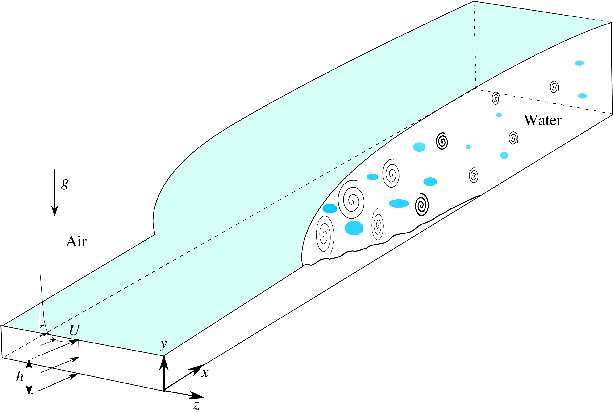
Schematic of a hydraulic jump, with
 $h$
as the inflow height and
 $U$
as the water inflow velocity. Air inflow velocity is a set to be the water inflow velocity minus a Blasius profile with
 ${\it\delta}_{99}=1.3h$
, in order to preserve the continuity of the velocity profile at the interface.

Figure 2 shows a schematic of the hydraulic jump and a coordinate system, with
 $x$
,
 $y$
and
 $z$
representing the streamwise, cross-flow and spanwise directions, respectively. The water inflow has a uniform velocity,
 $U$
, with height
 $h$
, and the jump occurs at some distance downstream of the inlet. In realistic scenarios, the problem involves a boundary layer on the bottom wall. Under the conditions that the displacement thickness of the boundary layer is much smaller than the inlet height,
 $h$
, the effects of the boundary layer on jump dynamics can be neglected. Since the focus of the present study is the wave breaking phenomena, we consider a simple canonical scenario in which the bottom boundary layer is neglected. Therefore, the bottom boundary is modelled as a slip wall on which only the no-penetration condition is enforced.
2.2 Dimensionless parameters
The presented setting involves three dimensionless parameters. The first parameter is the Froude number,
 $Fr=U/\sqrt{gh}$
, that indicates the relative importance of the inertial term in comparison to the gravitational term. The second parameter is the Weber number,
 $We={\it\rho}U^{2}h/{\it\sigma}$
, which indicates the importance of the surface tension force in terms of inertial forces. The third dimensionless parameter is the Reynolds number,
 $Re={\it\rho}Uh/{\it\mu}$
. However, for sufficiently high Reynolds number, the hydrodynamic instabilities in the hydraulic jump are inviscid as the velocity profile has an infliction point. As discussed in § 2.4 and appendix C, we hypothesize that low-order statistics, such as mean flow and kinetic energy, as well as rate of air entrainment are not sensitive to the Reynolds number in the regimes considered here.
In this work we consider a scenario with
 $Fr=2,We=1820$
and
 $Re=11\,000$
. Under such conditions, we can fully resolve the entire turbulence spectrum. Aside from turbulence, another important length scale that must be resolved is the Hinze scale, which indicates a threshold scale over which straining motions by turbulent eddies compete with the restoring surface tension force on bubbles. Based on a scaling analysis developed by Hinze and others (Kolmogorov Reference Kolmogorov1949; Hinze Reference Hinze1955) this threshold length is
 $$\begin{eqnarray}D_{H}=C\left(\frac{{\it\sigma}}{{\it\rho}}\right)^{3/5}{\it\varepsilon}^{-(2/5)},\end{eqnarray}$$
where
 ${\it\varepsilon}=2{\it\nu}\unicode[STIX]{x1D61A}_{ij}\unicode[STIX]{x1D61A}_{ij}$
is the turbulent kinetic energy dissipation,
 $\unicode[STIX]{x1D61A}_{ij}$
is the strain rate tensor and
 $C$
is a constant of order one, which was suggested to be
 $0.725$
by Hinze (Reference Hinze1955), using measurements of Clay (Reference Clay1940). The significance of the Hinze scale is that bubbles (or interface features) at scales above the Hinze scale can be broken into smaller pieces due to turbulence forces, but interface features below the Hinze scale are quickly restored due to the surface tension force. In other words, the Hinze scale indicates the minimum bubble size that can be generated due to fragmentation by turbulence. From the dissipation calculations that will be discussed later, the minimum Hinze scale is calculated to be of the order of
 $0.05h$
, which occurs just after the toe of the jump.
Two additional dimensionless parameters of this problem are the density ratio
 ${\it\rho}_{w}/{\it\rho}_{a}$
and the viscosity ratio
 ${\it\mu}_{w}/{\it\mu}_{a}$
. Considering an air–water system, these parameters are set to 831 and 50.5 respectively.
2.3 Numerical method
While the details of the employed numerical method together with validation test cases are presented in Le-Chenadec & Pitsch (Reference Le-Chenadec and Pitsch2013), we here briefly explain particular aspects in our simulation methodology.
The equations for conservation of mass and momentum are discretized on a structured uniform staggered mesh. Second-order accurate central schemes are used for spatial discretization and an explicit second-order Adams–Bashforth method is used for time integration. A two-step projection scheme coupled with the Ghost Fluid Method is used to solve a Poisson equation for pressure and to satisfy the divergence-free condition for the velocity field (Fedkiw et al. Reference Fedkiw, Aslam, Merriman and Osher1999).
Interface capturing is done with a hybrid Lagrangian Eulerian scheme (HyLEM) coupled with a level set equation (Le-Chenadec & Pitsch Reference Le-Chenadec and Pitsch2013). In this method, an advection equation is solved to track the volume fraction,
 $f$
,
 $$\begin{eqnarray}\frac{\partial f}{\partial t}+\boldsymbol{u}\boldsymbol{\cdot }\boldsymbol{{\rm\nabla}}f=0.\end{eqnarray}$$
This equation can be written for each moving control volume as
 $$\begin{eqnarray}\frac{\mathscr{D}_{m}}{\mathscr{D}_{m}t}\int _{{\it\Omega}_{m}}f\,\text{d}\boldsymbol{x}=0,\end{eqnarray}$$
where
 $\mathscr{D}_{m}$
denotes the material derivative and
 ${\it\Omega}_{m}$
is the control volume. We use an unsplit backward VOF scheme (Le-Chenadec & Pitsch Reference Le-Chenadec and Pitsch2013) to integrate this equation. In order to find the volume fraction of liquid in a cell at time step
 $n+1$
, first, piecewise linear interface reconstruction is done for time step
 $n$
for each cell. Assuming the undeformed Eulerian mesh corresponds to time step
 $n+1$
, we deform the mesh backward in time for one time step with the divergence-free velocity field. Each deformed mesh highlights fluid zones at time step
 $n$
that will advect to the undeformed Eulerian mesh by time step
 $n+1$
. Intersections of the deformed mesh with liquid zones will provide information of the volume of fluid in each cell at the next time step. Here, we have implicitly used (2.1) by assuming that the volume of moving fluid will not change.
While the aforementioned piecewise linear interface reconstruction method provides a robust framework for mass tracking, its accuracy is not sufficient for estimation of interface curvature and calculation of the surface tension force. To remedy this deficiency, we solve the level set equations that represent the interface as an isosurface of a smooth field (Osher & Sethian Reference Osher and Sethian1988). The employed combination of the level set method with a VOF formulation provides a setting to maintain accuracy of both mass conservation and curvature calculation. To maintain consistency between the two methods, at each time step the level set field is corrected towards a distance function obtained from the VOF filed with a relaxation parameter.
2.4 Computational domain and boundary conditions
The computational domain is set to
 $20.6h\times 4.2h\times 4.2h$
(
 $\text{length}\times \text{height}\times \text{width}$
), where
 $h$
is the inlet height of water. The length of the domain should be large enough that the effect of the outlet boundary condition on the middle of the flow is minimal. To ensure grid convergence of our results, we performed calculations using two different mesh resolutions. The fine resolution calculation employed
 $N_{x}\times N_{y}\times N_{z}=1280\times 256\times 256$
mesh points, while the coarse calculation used half of this grid resolution in each direction. We observed satisfactory agreement between the two simulations. The grid refinement study is presented in appendix B, and here we report only the fine simulation data.
As mentioned before, slip boundary conditions are implemented for the top and bottom walls in order to avoid complexities associated with thin boundary layers. Periodic boundary conditions are applied in the spanwise direction. A Dirichlet boundary condition is applied for the inflow and convective boundary condition is use for the outflow.
The inflow velocity is set equal to
 $U$
for the water phase. In the air phase the inflow velocity profile is set to
 $U$
minus a Blasius profile with
 ${\it\delta}_{99}=1.3h$
so that it reaches values close to zero near the top boundary.
To ensure that the position of the jump remains statistically stationary, we devised a numerical algorithm at the outflow boundary that guarantees zero numerical error in total mass transport for each phase. Such numerical conditions also guarantee the well posedness of the Poisson system for pressure. To this end, we first solve a convective equation to evolve velocities at the outflow boundary, as recommended by Pauley, Moin & Reynolds (Reference Pauley, Moin and Reynolds1990). In the limit of infinitely fine mesh and infinitely large outflow span, such treatment automatically guarantees the matching of total mass flow rates between inflow and outflow for each phase. In our simulation, however, due to the finite resolution and finite number of samples a small correction should be made. We use a velocity rescaling method (e.g. Kim & Moin Reference Kim and Moin1985) to guarantee the consistency of the mass flux for the water phase. In addition, we allow a similar small correction to the air outflow but only from
 $y=3h$
to
 $y=4h$
with a linear profile away from the water zone to ensure consistency of the air flux.
The employed numerical algorithm is validated against multiple tests in Le-Chenadec & Pitsch (Reference Le-Chenadec and Pitsch2013). In addition, we present a grid refinement study comparing the mean velocity and energy transfer terms between the fine and coarse meshes in appendix B. Furthermore, in appendix A, we present comparison of data from our simulation against experiments of Murzyn et al. (Reference Murzyn, Mouaze and Chaplin2005) and Murzyn et al. (Reference Murzyn, Mouaze and Chaplin2007) on air entrainment and interface length scales. The experimental data selected has a Froude number and Weber number matching those in our simulation. There is a mismatch in the Reynolds number due to prohibitive cost of DNS at the realistic
 $Re=88\,000$
. However, given that the flows considered do not involve boundary layers, the only role of Reynolds number (dimensionally varying fluid viscosity while keeping everything else fixed) is to control the extent of cascade of turbulence to small scales. Therefore, we hypothesize that as long as the Kolmogorov scale of turbulence remains smaller than the Hinze scale, the low-order flow statistics as well as bulk air entrainment rate remain insensitive to the Reynolds number. While we leave this hypothesis open for future investigations, here we present in appendix C evidence of insensitivity of the flow and air entrainment statistics on the system Reynolds number.
In contrary to our hypothesis, physical experiments suggest that air entrainment statistics are dependent on the Reynolds number (Chanson Reference Chanson2007b
; Murzyn & Chanson Reference Murzyn and Chanson2008). We attribute this difference of observations on two factors: (i) in an experiment, it is not possible to maintain
 $Fr$
number fixed while controlling
 $Re$
independent of
 $We$
, therefore some of the influence observed in experiments maybe in fact due to change in
 $We$
, and (ii) in realistic experiments the thickness of the bottom boundary layer is controlled by
 $Re$
, while in the canonical setting investigated here the dynamical effects of the bottom boundary layer are not included. Next, we present results from statistical analysis of our calculations.
3 Flow statistics
In this section we have used the inlet height,
 $h$
, inlet velocity,
 $U$
and water density,
 ${\it\rho}_{w}$
, to non-dimensionalize all of the presented variables. Statistical averaging is performed over 120 time units after the simulation reached fully turbulent conditions. All quantities reported are averaged in time and in the spanwise direction.
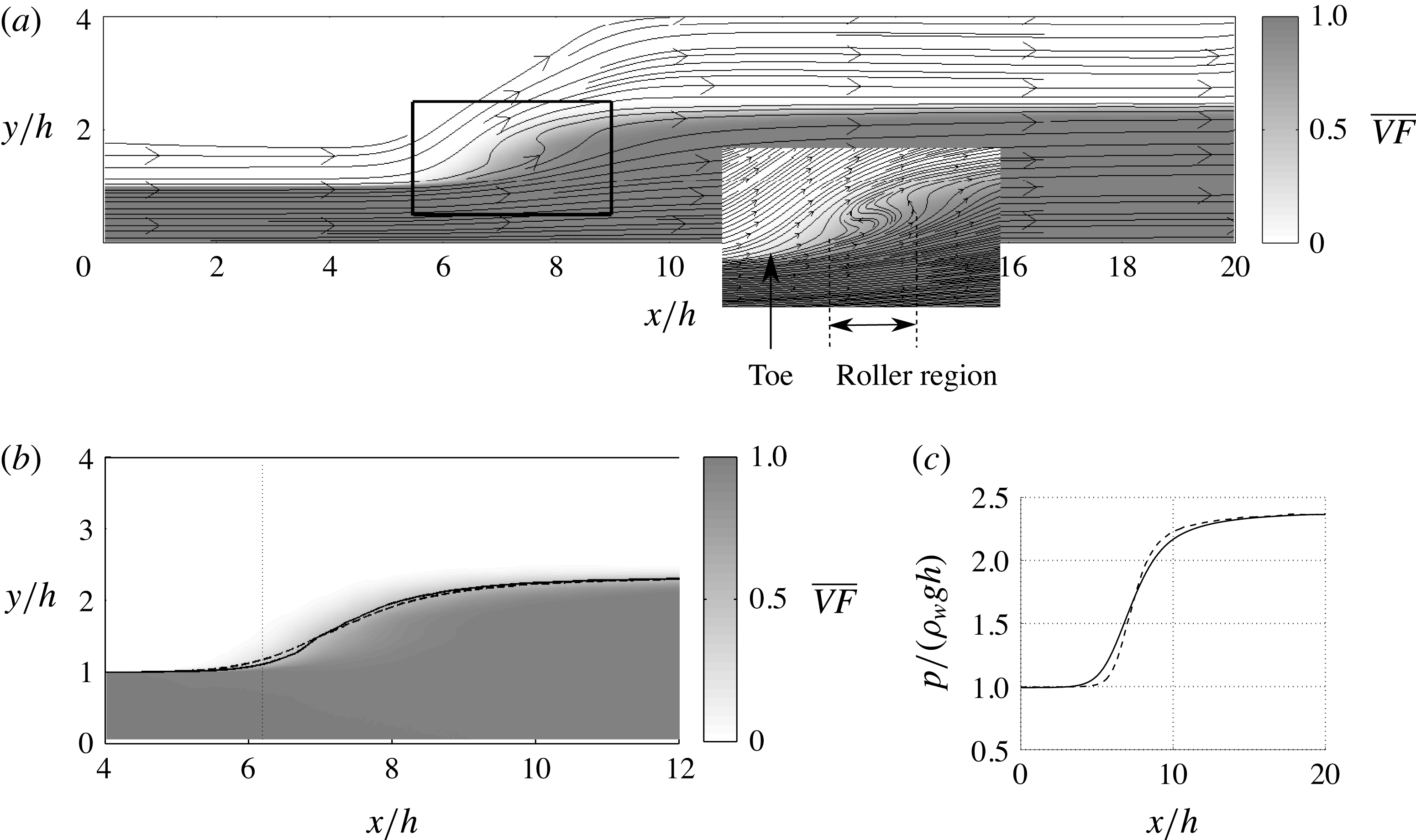
Figure 3(a) demonstrates the average volume fraction of water as well as the streamlines of averaged velocities. In the inset, the streamlines indicate the presence of a roller right after the toe of the jump, where the flow recirculates. In figure 3(b) two different methods for defining the mean interface position are shown. One is the isocontour of the volume fraction at
 $\overline{VF}=0.5$
and the other is obtained by integrating the volume fraction in the
 $y$
direction from the bottom to the top computational boundaries, which henceforth we call
 $y_{fs}$
. The two profiles are very close to each other.
(a) Time- and spanwise-averaged volume fraction of water and velocity streamlines. (b) Two methods for defining the average interface position are compared: the isocontour of the volume fraction at
 $\overline{VF}=0.5$
(——) and the integral of the volume fraction in the
 $y$
direction,
 $y_{fs}$
(– –). The vertical dashed line indicates the position of the toe for the jump at
 $x/h=6.2$
, where the mean interface height is increased by
 $10\,\%$
of the inlet height. (c) Bottom wall pressure distribution. Total pressure (——), hydrostatic pressure,
 ${\it\rho}_{w}gy_{fs}$
(– –).

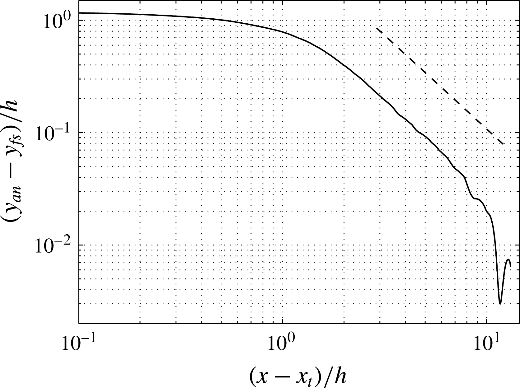
Convergence of the height of the free surface to the analytical value of
 $y_{an}=(-1+\sqrt{1+8Fr^{2}})/2$
after the toe of a hydraulic jump with
 $Fr=2$
. The straight dashed line shows the slope of
 $-5/3$
.

We define the position of the toe of the jump as the location where the volume fraction isocontour,
 $\overline{VF}=0.5$
, is elevated by
 $10\,\%$
above the inflow height. Based on coordinates shown in figure 3, which use the inflow boundary of the computational domain as the origin, the location of the toe is at
 $x_{t}/h=6.2$
. Note that even with the same computational mesh, the location of the jump depends on the initial condition, specifically on how much water is included in the domain initially. Therefore, the jump location measured from the computational inlet is not a computationally reproducible quantity (for reproducible simulations, the initial water in the domain must match a jump represented by a linear ramp starting at
 $x/h=6.10$
and ending at
 $x/h=12.88$
). However, any statistical quantity with coordinate relative to the toe location must be reproducible. Therefore, in the rest of the paper we highlight coordinates relative to the toe location by reporting
 $x-x_{t}$
. From the figure, it is clear that the interface ‘jump’ occurs over a large streamwise length. The steepest rise spans over
 ${\sim}2h$
and a more gradual rise continues over a distance of
 $O(10h)$
downstream of the jump. As shown in figure 4, the free surface height asymptotes to the analytical solution with the difference decaying with a power law of
 $-5/3$
. At the end of the domain, as the difference between the interface height and the analytical value becomes smaller than the statistical errors, some oscillations are observed. At the end of the computational domain, which is
 $14h$
downstream of the toe, the mean free surface reaches the asymptotic value.
The pressure distribution at the bottom wall is shown in figure 3(c). The hydrostatic pressure is computed from the integral of the mean weight of the water column above the surface, equal to
 ${\it\rho}_{w}gy_{fs}$
. The total pressure deviates slightly from the hydrostatic value in the region of energy exchange (
 $3<x/h<14$
). Beyond this region, hydrostatic pressure can be a good approximation for the total pressure at the wall.
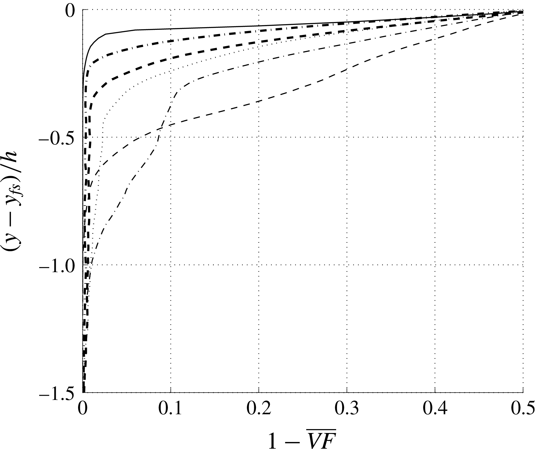
Figure 5 shows the cross-section profiles of the predicted void fraction at different distances from the toe. The depth of penetration of air is measured as
 $y-y_{fs}(x)$
. The penetration depth increases and reaches a maximum at a streamwise location two inlet heights downstream of the jump at around
 $x/h=8$
. After this stage the penetration depth decreases due to buoyant rise of the entrained air.
Cross-sectional profiles of mean void fraction:
 $(x-x_{t})/h=0$
(——), 1.0 (– –), 2.0 (— ⋅ —), 3.0 (
 $\cdots \cdots$
), 4.0 (– –) and 6.0 (— ⋅ —). Here
 $y_{fs}$
is the vertical location of the interface at the corresponding
 $x/h$
.

3.1 Velocity mean and fluctuations
Since the velocity field is continuous from air to water, we have used time and spanwise averaging according to
 $$\begin{eqnarray}\displaystyle & \displaystyle \overline{u}=\int _{0}^{\text{T}}\int _{0}^{L_{z}}u\,\text{d}z\,\text{d}t/(TL_{z}) & \displaystyle\end{eqnarray}$$
 $$\begin{eqnarray}\displaystyle & \displaystyle u_{rms}^{\prime }=\sqrt{\overline{(u-\overline{u})^{2}}}. & \displaystyle\end{eqnarray}$$
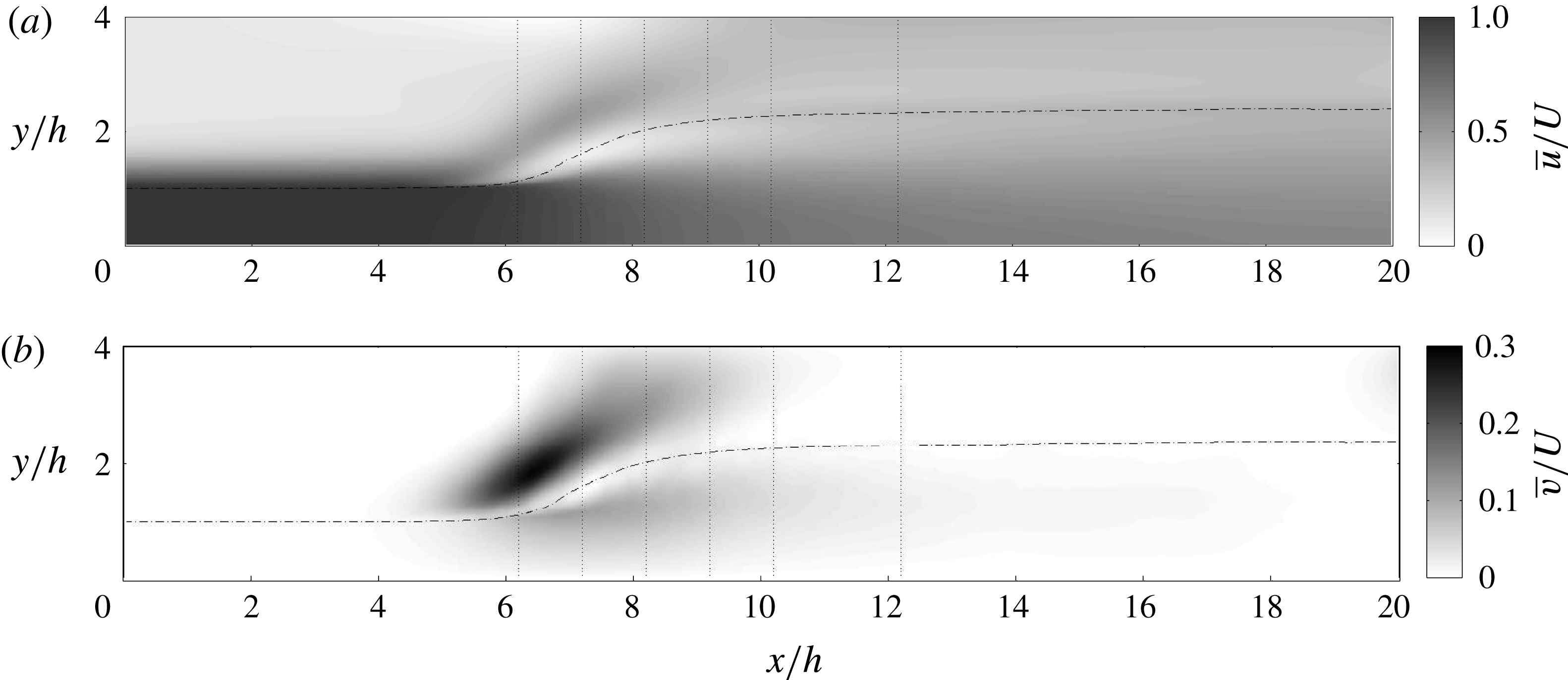
Figure 6 shows the mean streamwise and vertical velocities in the domain. The core of the roller region is revealed by an almost stagnant flow after the toe of the jump. At the toe of the jump, the vertical velocity is the largest, specifically on the air side, due to the upward redirection of the flow by the jump. The vertical dotted lines are the positions where the mean velocity profiles are plotted in figure 7.
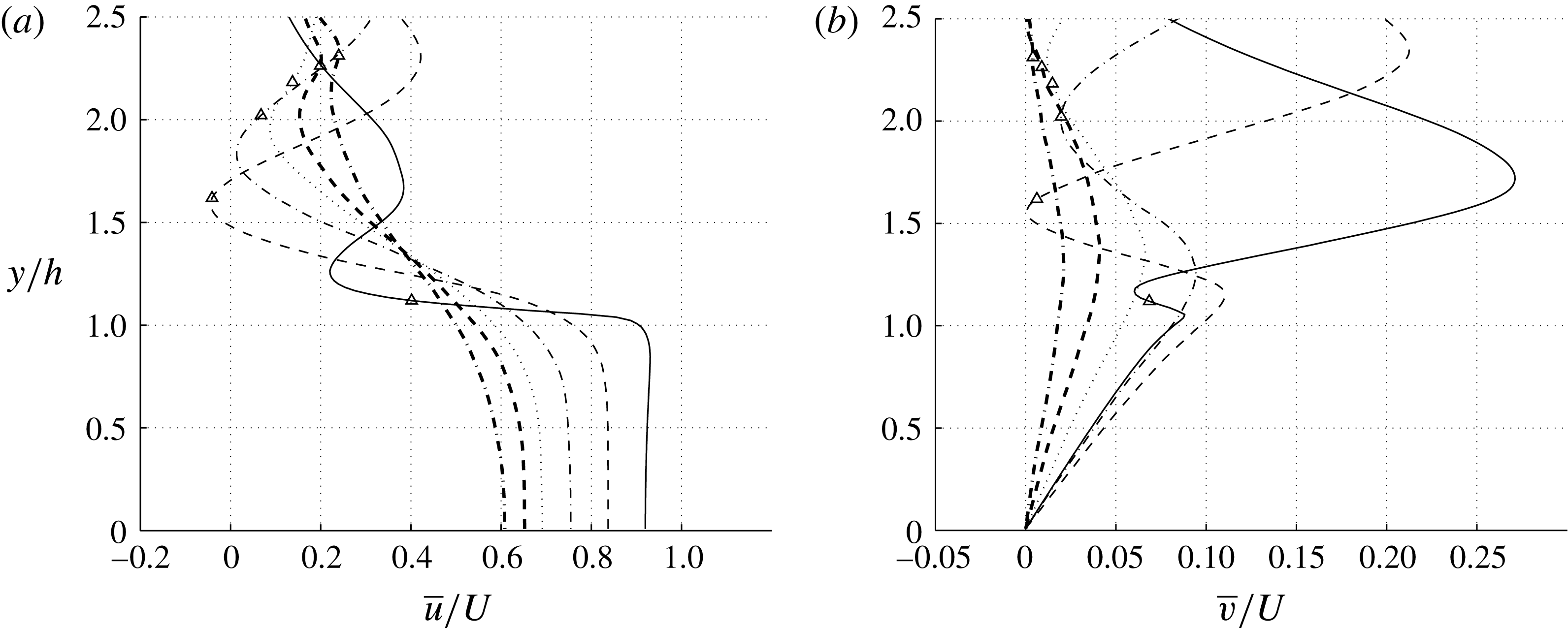
Figure 7 shows the mean velocity profiles as a function of
 $y$
at different streamwise positions of the jump. The markers on the profiles show the mean position of the interface defined by
 $\overline{VF}=0.5$
in the corresponding streamwise location. As one moves in the direction of the flow, the maximum mean streamwise velocity decreases. On the air side, the flow is accelerated due to the presence of the jump, and a jet-like profile is formed. In the normal velocity profiles, two peaks (one in each phase) are detected due to the redirection of the flow in the roller region, and these are separated by the position of the interface, where the flow is in a near-stagnant condition.
Time- and spanwise-averaged velocity contours. The vertical dotted lines are the positions where the cross-sectional velocity profiles are shown in the next figure. The dash-dotted line corresponds to
 $\overline{VF}=0.5$
.

Mean velocity profiles for different streamwise positions of the flow:
 $(x-x_{t})/h=0$
(——), 1.0 (– –), 2.0 (— ⋅ —), 3.0 (
 $\cdots \cdots$
), 4.0 (– –) and 6.0 (— ⋅ —). The symbols show the position of
 $\overline{VF}=0.5$
.

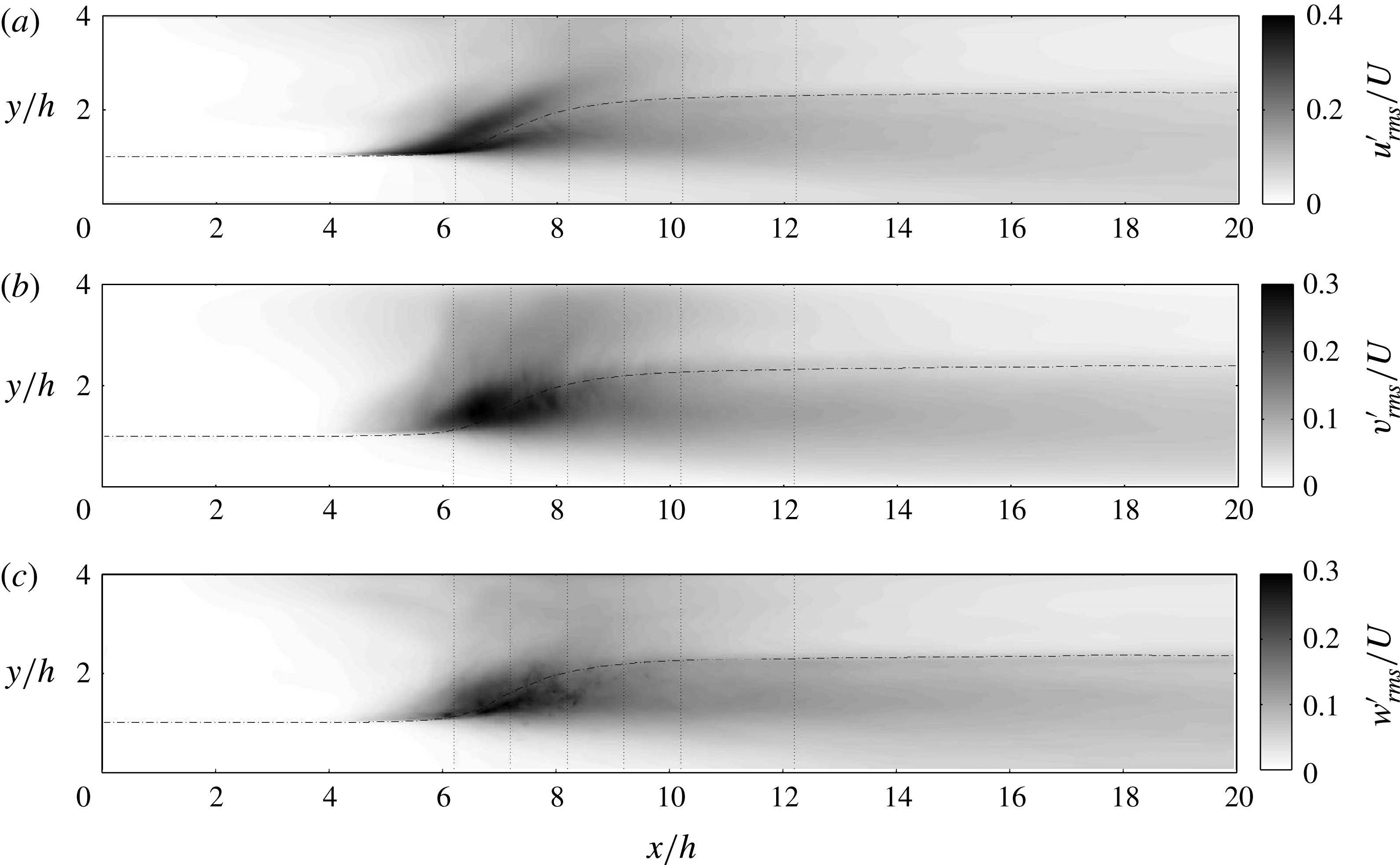
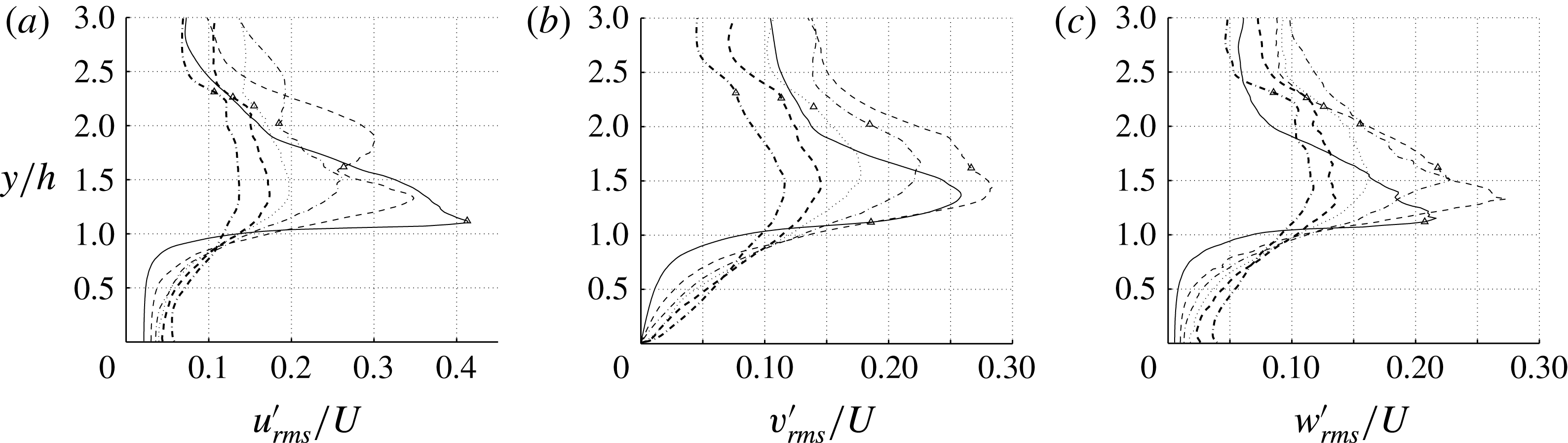
Time- and spanwise-averaged root mean square of velocity fluctuations. The vertical dotted lines are the positions where the cross-sectional profiles are shown in the next figure. The dash-dotted line corresponds to
 $\overline{VF}=0.5$
.

Root-mean-square profiles of velocity fluctuations for different streamwise positions of the flow:
 $(x-x_{t})/h=0$
(——), 1.0 (– –), 2.0 (— ⋅ —), 3.0 (
 $\cdots \cdots$
), 4.0 (– –) and 6.0 (— ⋅ —). The symbols show the position of
 $\overline{VF}=0.5$
.

Figure 8 shows the root-mean-square values of velocity fluctuations. The maximum velocity fluctuations are associated with the recirculation region, due to its highly energetic dynamics, as well as instantaneous fluctuations in local jump conditions. Furthermore, as one moves downstream, the streamwise fluctuations are initially larger than those in the other two directions. This is to be expected since the initial flow is parallel in the
 $x$
-direction, and a slight fluctuation in the jump toe location can manifest itself in terms of
 $u_{rms}^{\prime }$
. However, once turbulence develops fluctuations in all three directions become comparable. This transition occurs within
 ${\sim}2h$
downstream of the toe.
Figure 9 shows the profiles of velocity fluctuations for different streamwise positions. Close to the toe, the maximum fluctuation occurs near the interface. In these regions, the mean flow (figure 7) strongly resembles that of a separated shear layer and is highly susceptible to Kelvin–Helmholtz-type instabilities. As one moves downstream, the height of the peak velocity fluctuations shifts slightly upward, but at the rate slower than that of the interface itself. After a distance of approximately
 $2h$
, once the 3-D turbulence is well established, the peak location of fluctuations shifts up to
 $y\simeq 1.5h$
, which is roughly the average of the inlet height and outlet height. The location of the peak does not change much downstream of this location, and all three components of velocity peak at roughly around the same location and decay together as fluid is transported downstream.
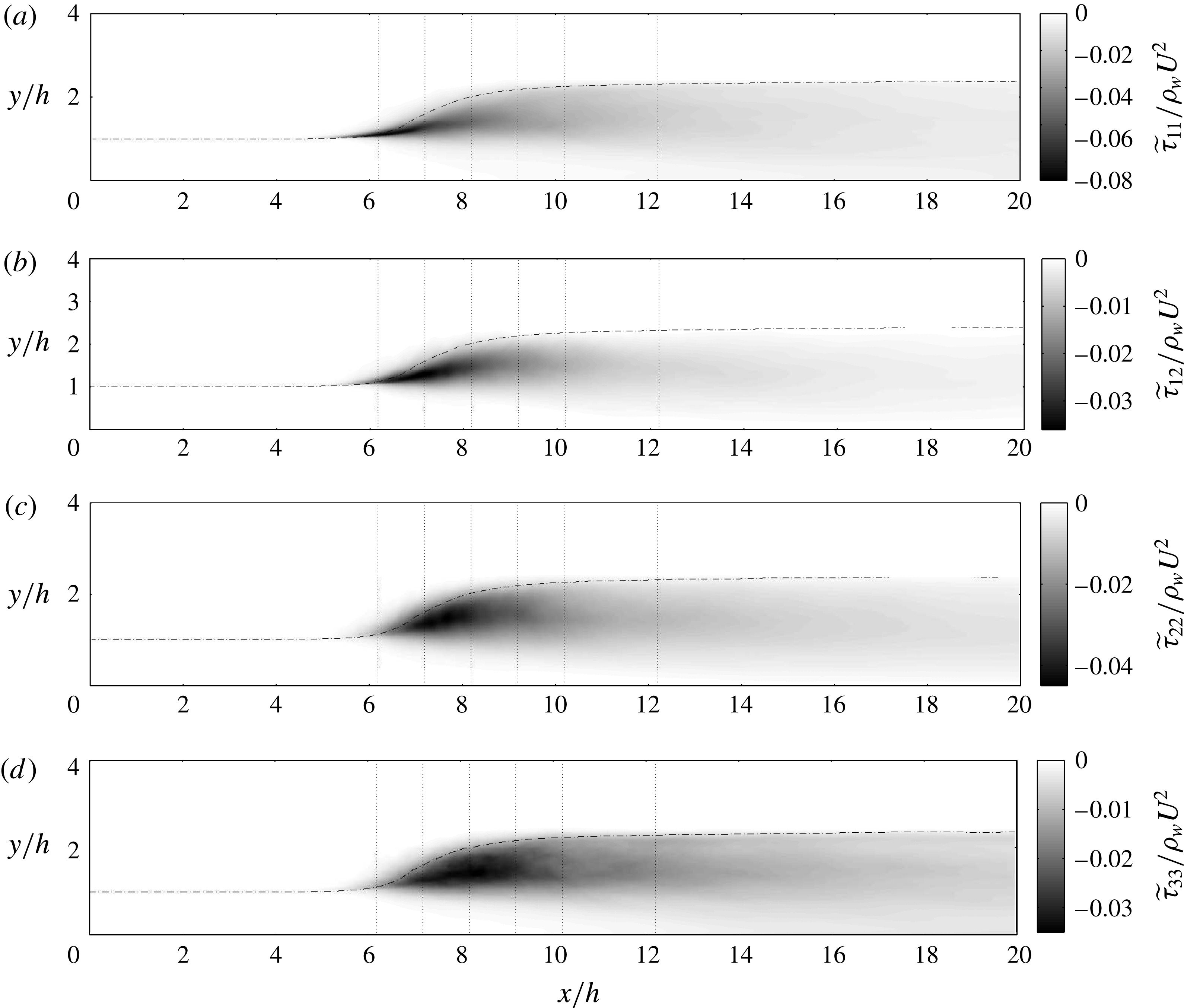
Time and spanwise Favre-averaged turbulent Reynolds stresses,
 $\widetilde{{\it\tau}}_{ij}=-\overline{{\it\rho}}\widetilde{u_{i}^{\prime \prime }u_{j}^{\prime \prime }}$
. The vertical dotted lines are the positions where the cross-sectional profiles are shown in the next figure. The dash-dotted line corresponds to
 $\overline{VF}=0.5$
.

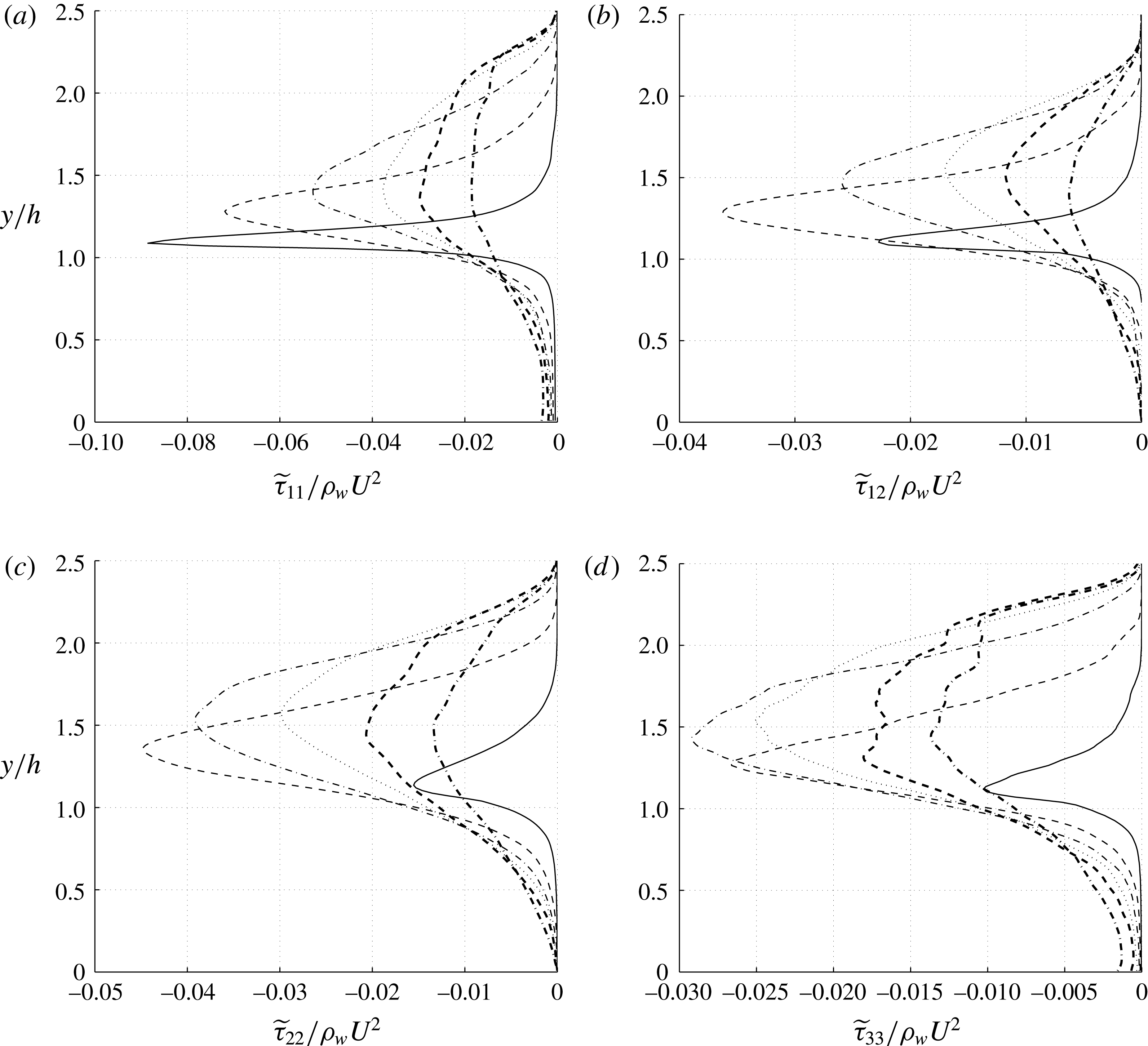
Reynolds stress profiles,
 $\widetilde{{\it\tau}}_{ij}=-\overline{{\it\rho}}\widetilde{u_{i}^{\prime \prime }u_{j}^{\prime \prime }}$
in different streamwise locations:
 $(x-x_{t})/h=0$
(——), 1.0 (– –), 2.0 (— ⋅ —), 3.0 (
 $\cdots \cdots$
), 4.0 (– –) and 6.0 (— ⋅ —).

3.2 Reynolds stresses
The equations for the Favre-averaged mean momentum for variable density flows are
 $$\begin{eqnarray}\frac{\partial (\overline{{\it\rho}}\widetilde{U_{i}})}{\partial t}+\frac{\partial (\overline{{\it\rho}}\widetilde{U_{i}}\widetilde{U_{j}})}{\partial x_{j}}=\overline{{\it\rho}}\widetilde{f_{Si}}-\frac{\partial \overline{p}}{\partial x_{i}}-\frac{\partial (\overline{{\it\rho}}\widetilde{{u_{i}}^{\prime \prime }{u_{j}}^{\prime \prime }})}{\partial x_{j}}+\frac{\partial \overline{{\it\tau}_{ij}}}{\partial x_{j}},\end{eqnarray}$$
where velocity is decomposed as
 $U_{i}=\widetilde{U_{i}}+u_{i}^{\prime \prime }$
, where
 $\widetilde{U_{i}}=\overline{{\it\rho}U}/\overline{{\it\rho}}$
is the Favre-averaged velocity and
 ${\it\tau}_{ij}={\it\mu}(\partial U_{i}/\partial x_{j}+\partial U_{j}/\partial x_{i})$
is the molecular shear stress tensor. The Reynolds stress tensor is defined as
 $$\begin{eqnarray}\widetilde{{\it\tau}}_{ij}=-\overline{{\it\rho}}\widetilde{u_{i}^{\prime \prime }u_{j}^{\prime \prime }},\end{eqnarray}$$
which represents the effect of fluctuating velocities on the mean momentum transport. Any reduced model for momentum transport in hydraulic jumps, such as a RANS model, must close the Reynolds stresses in terms of mean quantities. Statistical homogeneity of the flow in the spanwise direction results in zero Reynolds stresses for the
 $\widetilde{{\it\tau}}_{13}$
and
 $\widetilde{{\it\tau}}_{23}$
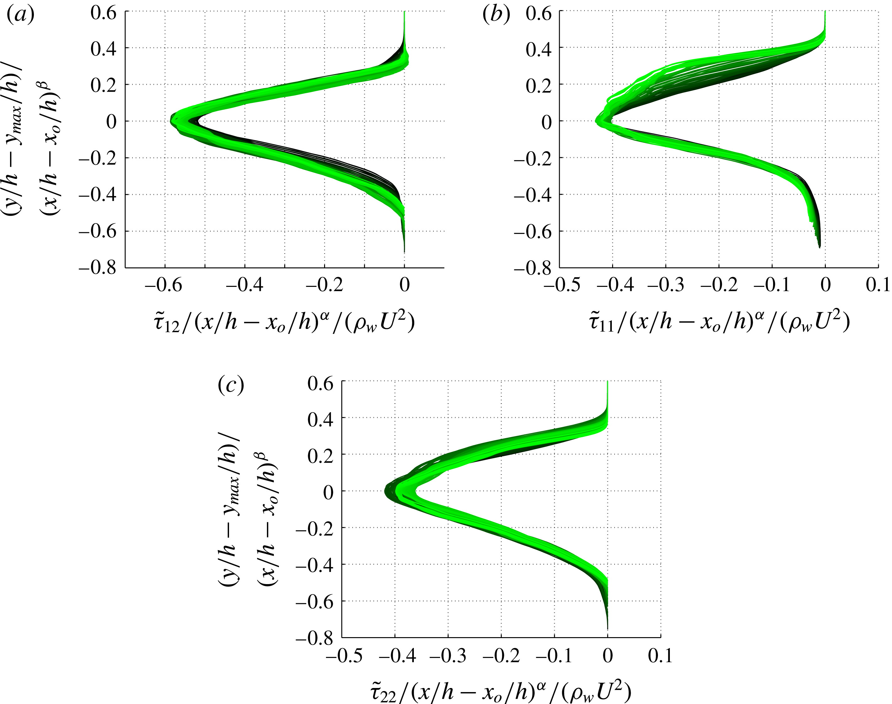
components. The remaining components of the Reynolds stress are non-zero. Figure 10 demonstrates a contour plot of these components, and cross-sectional profiles at multiple streamwise sections are shown in figure 11.
The statistical error of the mean for velocity, fluctuations and Reynolds stresses is estimated by computing the standard deviation of these quantities, obtained over multiple temporal windows, divided by the square root of the number of windows, times a factor of
 $1.96$
for
 $95\,\%$
confidence. The maximum statistical error of the mean in the domain for all of the mentioned quantities is computed to be within
 $\pm 10\,\%$
accuracy.
At the toe of the jump,
 $\widetilde{{\it\tau}}_{11}$
is the dominant component of the Reynolds stress, and the other components are much smaller. Downstream of the flow at
 $(x-x_{t})/h=6$
, all the components of the Reynolds shear stress are close to each other and the flow becomes more isotropic. Similar to the velocity fluctuations, the position of the peak of the Reynolds stress profiles also moves slightly up after the toe and stays fairly stationary at
 $y/h\simeq 1.5$
downstream of the flow. As expected, in the water side, the sign of
 $\widetilde{{\it\tau}}_{12}$
is the same as the vertical gradient of the streamwise velocity component
 $\text{d}\widetilde{U}/\text{d}y$
, which is negative. It becomes maximum at
 $(x-x_{t})/h=1$
, which is in the middle of the roller region of the jump.
4 One-dimensional energy balance
The instantaneous pointwise kinetic energy equation can be written as
 $$\begin{eqnarray}\frac{\partial {\it\rho}\frac{1}{2}u_{i}u_{i}}{\partial t}+\frac{\partial {\it\rho}u_{j}\frac{1}{2}u_{i}u_{i}}{\partial x_{j}}=-\frac{\partial pu_{i}}{\partial x_{i}}+{\it\mu}\frac{\partial ^{2}\frac{1}{2}u_{i}u_{i}}{\partial x_{j}\partial x_{j}}-{\it\mu}\frac{\partial u_{i}}{\partial x_{j}}\frac{\partial u_{i}}{\partial x_{j}}+{\it\rho}u_{i}g_{i}+f_{Si}u_{i}.\end{eqnarray}$$
In order to obtain a 1-D energy equation, we integrate (4.1) in a control volume of
 $V=[x^{(1)},x^{(2)}]\times [0,L_{y}]\times [0,L_{z}]$
, where
 $x^{(1)}$
and
 $x^{(2)}$
are two streamwise locations. Averaging in time one obtains
 $$\begin{eqnarray}\displaystyle & & \displaystyle \displaystyle \frac{\partial }{\partial t}\int _{V}\overline{\left({\it\rho}\frac{1}{2}u_{i}u_{i}+{\it\rho}yg\right)}\,\text{d}V+\int _{0}^{Ly}\int _{0}^{Lz}\overline{\left[\underbrace{\frac{1}{2}{\it\rho}u_{i}u_{i}}_{\text{kinetic}\,\text{energy}}+\underbrace{{\it\rho}yg}_{\text{potential}\,\text{energy}}+\underbrace{p}_{\text{pressure}}\right]u_{1}}\,\text{d}z\,\text{d}y|_{x^{(2)}-x^{(1)}}\nonumber\\ \displaystyle & & \displaystyle \displaystyle \quad =\int _{0}^{Ly}\int _{0}^{Lz}{\it\mu}\overline{\frac{\partial {\textstyle \frac{1}{2}}u_{i}u_{i}}{\partial x}}\,\text{d}z\,\text{d}y|_{x^{(2)}-x^{(1)}}-\underbrace{\int _{V}{\it\mu}\overline{\frac{\partial u_{i}}{\partial x_{j}}\frac{\partial u_{i}}{\partial x_{j}}}\,\text{d}V}_{\text{dissipation}}+\int _{V}\overline{f_{Si}u_{i}}\,\text{d}V.\end{eqnarray}$$
In deriving the equation above, we have used the identity below, which can be derived from continuity
 $$\begin{eqnarray}\int {\it\rho}u_{i}g_{i}\,\text{d}V=\int \frac{\partial {\it\rho}x_{i}g_{i}}{\partial t}\,\text{d}V+\int \frac{\partial {\it\rho}u_{j}x_{i}g_{i}}{\partial x_{j}}\,\text{d}V,\end{eqnarray}$$
where
 $|_{x^{(2)}-x^{(1)}}$
indicates the difference of the integral between
 $x^{(2)}$
and
 $x^{(1)}$
. The time-derivative term can be assumed to be zero, since the flow is statistically stationary. The surface integral on the left-hand side has three terms, namely, net kinetic energy flux, net potential energy flux and net pressure work in a control volume of length
 ${\rm\Delta}x=x^{(2)}-x^{(1)}$
in the streamwise direction. On the right-hand side, the terms represent net viscous flux, energy dissipation and surface tension energy. From the results of our simulation we have determined that the net viscous flux term and the surface tension energy term are negligible compared to the other terms. These two terms are of the same order, but they are two orders of magnitude smaller than the other terms.
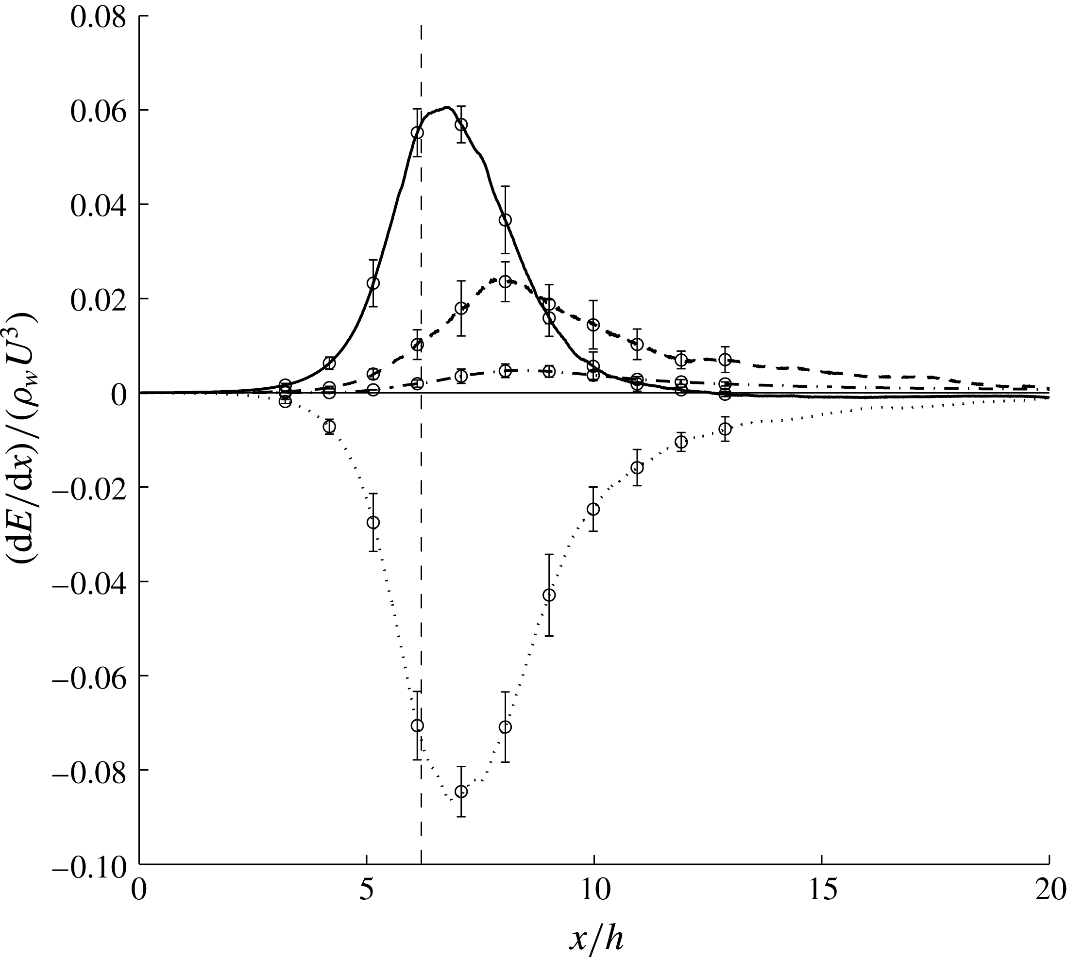
Transfer of kinetic energy to other forms of energy as a function of streamwise location. The plots represent exchange rates due to kinetic energy (
 $\cdots \cdots$
), potential energy (– –), pressure work (——) and dissipation (— ⋅ —). The error bars show the statistical errors of the calculations. The vertical dashed line shows the position of the toe at
 $x/h=6.2$
.

Figure 12 shows quantitatively the rate at which kinetic energy transfers to potential energy, pressure energy and dissipation, at each streamwise station of the flow. For this purpose, we computed the streamwise divergence of each flux, and report the exchange in terms of power per unit of streamwise length per unit of spanwise length. These exchange terms are defined as
kinetic energy exchange rate:
 $[\int _{0}^{Lz}\int _{0}^{Ly}\overline{({\it\rho}u_{i}u_{i}u_{1})/2}\,\text{d}y\,\text{d}z|_{x^{(2)}-x^{(1)}}]/({\rm\Delta}xL_{z})$
,
potential energy exchange rate:
 $[\int _{0}^{Lz}\int _{0}^{Ly}\overline{{\it\rho}gyu_{1}}\,\text{d}y\,\text{d}z|_{x^{(2)}-x^{(1)}}]/({\rm\Delta}xL_{z})$
,
pressure energy exchange rate:
 $[\int _{0}^{Lz}\int _{0}^{Ly}\overline{pu_{1}}\,\text{d}y\,\text{d}z|_{x^{(2)}-x^{(1)}}]/({\rm\Delta}xL_{z})$
,
dissipation rate:
 $\left[\int _{V}{\it\mu}\overline{(\partial u_{i}/\partial x_{j})(\partial u_{i}/\partial x_{j})}\,\text{d}V\right]\!/({\rm\Delta}xL_{z})$
,
where
 $L_{z}$
is the length of the domain in the spanwise direction. The error bars in the figure show the statistical error of the calculations for kinetic energy, potential energy and pressure work and for dissipation, the error bars are based on the discrepancy between the coarse and fine meshes. The summation of these four curves is zero within the statistical errors.
The plots in figure 12 reveal aspects about the energy transfer process that were previously unknown in existing 1-D theories. Specifically, these results show the order and streamwise extent of various exchange processes. As shown, the exchange process starts at approximately two inlet heights upstream of the toe of the jump, which can be explained by the fact that the instantaneous toe location has some oscillations relative to the defined mean location. As the flow advects downstream, the first mode of energy exchange involves transfer of kinetic energy to pressure energy. At the toe (
 $x/h=6.2$
) the transfer to pressure energy is close to its peak, while there is some minor transfer to potential energy and dissipation. The transfer to potential energy and dissipation rate peak at approximately one and a half inlet heights downstream of the toe at
 $x/h\sim 7.5$
, while the dominant transfer is still to pressure work. After approximately two inlet heights downstream of the toe, the transfer to pressure work term drops significantly and most of the kinetic energy transfers to potential energy, with some transfer to dissipation.
Although the dissipation term is relatively small compared to the other terms, it decays more slowly, and stays at the order of its peak value for a long distance downstream of the jump. The pressure work decays the fastest and almost reaches zero after
 $x/h\sim 11$
. Similar to dissipation, potential energy has a long tail, which is an indication that the height of the jump has a gradual increase to its asymptotic value for large distances after the toe. This fact justifies the choice of our large computational domain. From the analytical 1-D model for hydraulic jumps, which assumes uniform inflow and outflow velocity profiles with the Belanger relationship for the ratio of the water heights, we can compute the energy states far upstream and downstream of the jump. According to this solution, the net change in the total sum of kinetic, pressure, and potential energy per unit spanwise length is
 $(E_{2}-E_{1})/{\it\rho}_{w}U^{3}h=-0.067$
. From our calculations we obtain a value of
 $(E_{2}-E_{1})/{\it\rho}_{w}U^{3}h=-0.051$
. In other words, only approximately
 $76\,\%$
of the total dissipation occurs within the computational domain, which includes distances up to 14 inlet heights downstream of the jump (
 $x/h=20$
).
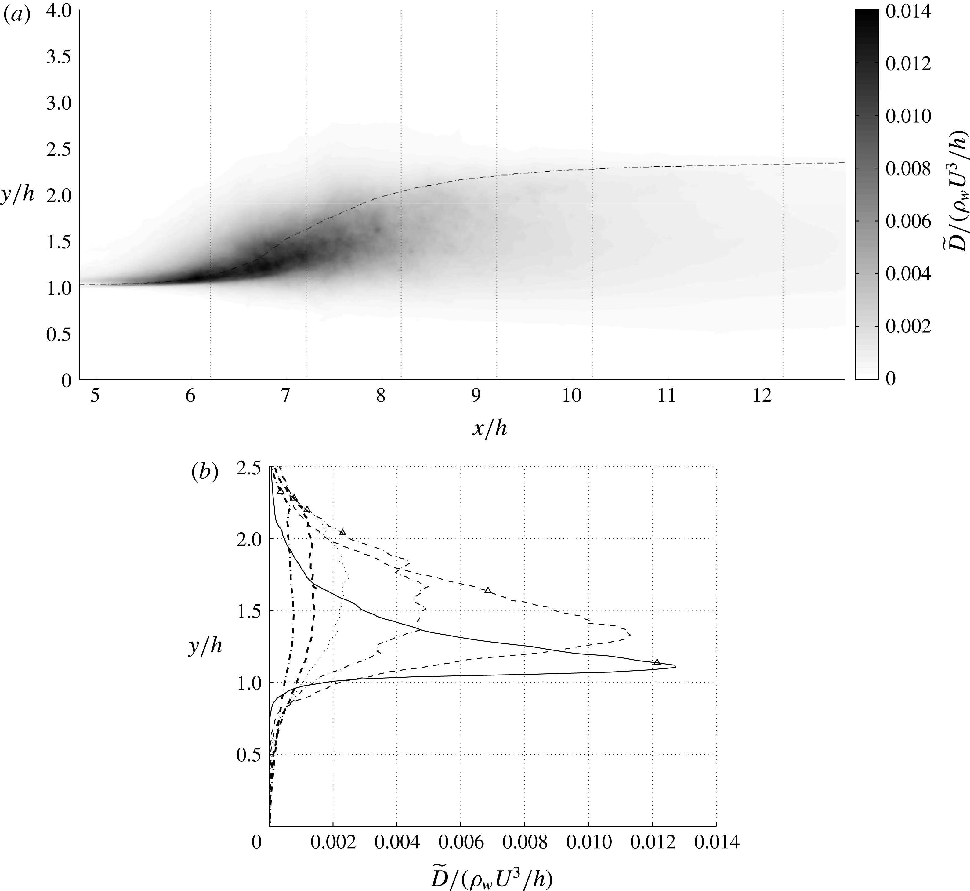
Turbulent dissipation
 $\widetilde{D}=\overline{{\it\tau}_{ij}(\partial u_{i}^{\prime \prime }/\partial x_{j})}$
in the domain and its cross-sectional profiles in different streamwise locations:
 $(x-x_{t})/h=0$
(——), 1.0 (– –), 2.0 (— ⋅ —), 3.0 (
 $\cdots \cdots$
), 4.0 (– –) and 6.0 (— ⋅ —). The dash-dotted line in (a) and the symbols in (b) correspond to
 $\overline{VF}=0.5$
.

The presented results provide insight, as well as quantitative validation benchmarks, for the development of reduced-order models for breaking waves in applications such as ocean and river flows, as well as dam flow models. Specifically, these data provide insight into modelling of, often unclosed, dissipation terms by highlighting their long tail after nonlinear breaking events.
5 Dissipation field and estimation of Hinze scale
As mentioned in the introduction, the turbulent kinetic energy dissipation rate is a key parameter that affects bubble size distribution in the entrained air in bubbly flows (Hinze Reference Hinze1955; Garrett et al. Reference Garrett, Li and Farmer2000). The dissipation term in the Favre-averaged turbulent kinetic energy equation reads
 $$\begin{eqnarray}\widetilde{D}=\overline{{\it\tau}_{ij}\frac{\partial u_{i}^{\prime \prime }}{\partial x_{j}}},\end{eqnarray}$$
where
 $u_{i}^{\prime \prime }$
is the Favre-averaged fluctuation velocity and the bar represents the spanwise- and time-averaging operator here. Figure 13 shows the turbulent kinetic energy dissipation in the domain as well as their cross-sectional profile for different locations of the jump. Similar to the other turbulence statistics, the maximum dissipation occurs at the toe of the jump and very close to the interface. Further downstream, the peak dissipation occurs below the interface but at a height higher than
 $h$
. Far downstream, peak dissipation occurs at a height of
 $y/h\simeq 1.5$
measured from the bottom boundary.
Equation (2.4) provides a scaling estimate for the minimum bubble size, called the Hinze scale. Based on the computed dissipation field, the minimum Hinze scale for the flow is around
 $D_{H}=0.05h$
(dimensionally
 $2.8~\text{mm}$
). Downstream of the flow as the dissipation drops, the Hinze scale increases to
 $D_{H}=0.17h$
. While we defer detailed investigation of bubble size distribution to a future publication, we note here that one factor contributing to bubble size distribution can be variation in the dissipation field sampled by different pieces of the entrained air. This insight can be used to correct the existing theories of bubble size distribution (Garrett et al.
Reference Garrett, Li and Farmer2000), which use only one dissipation number to infer bubble size by assuming homogeneous turbulence.
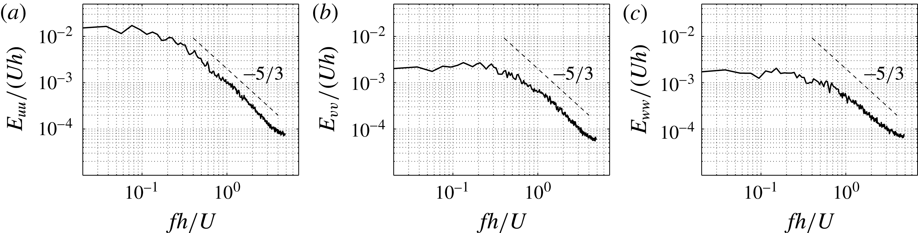
Energy spectrum of velocity components for
 $(x-x_{t})/h=0$
,
 $y/h=1$
: (a)
 $u$
spectrum; (b)
 $v$
spectrum; (c)
 $w$
spectrum.

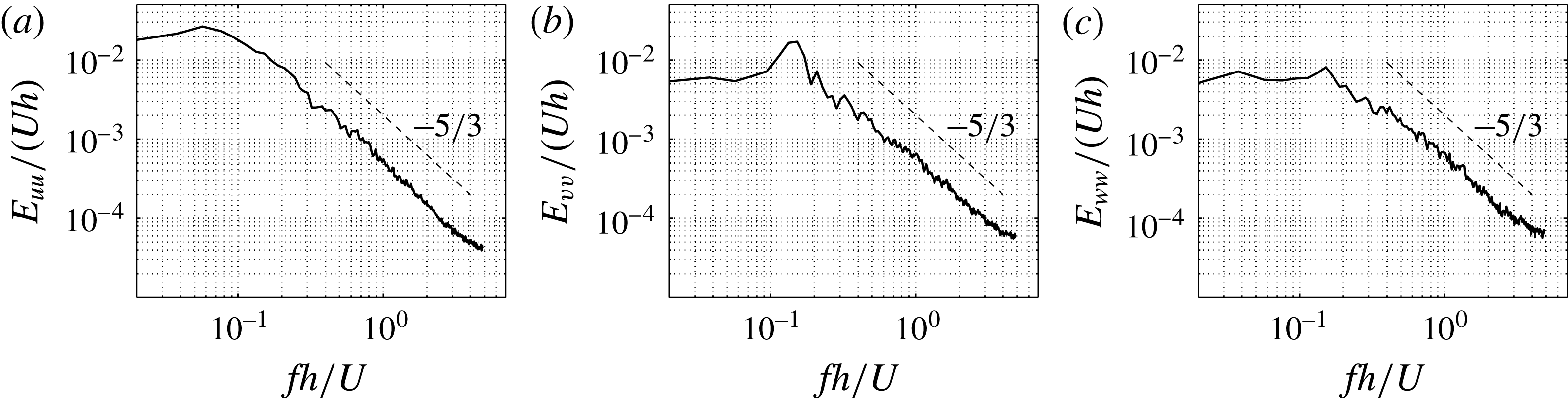
Energy spectrum of velocity components for
 $(x-x_{t})/h=2$
,
 $y/h=1.1$
: (a)
 $u$
spectrum; (b)
 $v$
spectrum; (c)
 $w$
spectrum.

6 Energy spectra
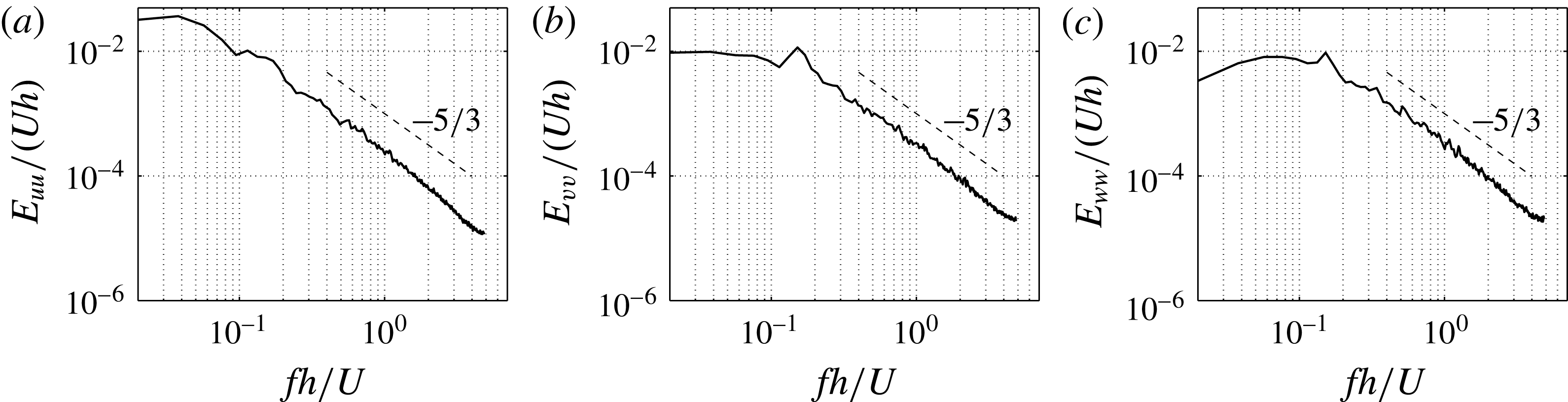
Temporal energy spectra of the velocity components are computed in figures 14, 15 and 16 for locations
 $(x-x_{t})/h=0,2$
and
 $4$
, respectively. The slope of
 $-5/3$
is observed for the inertial range, suggesting that even though the problem involves two-phase flow phenomena and transport of bubbles, the energy transfer process still involves a Kolmogorov-type spectrum. Furthermore, a distinct frequency peak can be distinguished, which is more evident in the spectra of the vertical velocity at locations
 $(x-x_{t})/h=2$
and
 $(x-x_{t})/h=4$
. Our more careful investigations indicate that this frequency peak is due to a vortex-shedding phenomenon originating at the toe of the jump. This phenomenon was previously observed in qualitative visualization of Long et al. (Reference Long, Rajaratnam, Steffler and Smy1991a
) for hydraulic jumps, and in the experiments of Rodriguez-Rodriguez et al. (Reference Rodriguez-Rodriguez, Marugan-Cruz, Aliseda and Lasheras2011) for steady breakers.
Energy spectrum of velocity components for
 $(x-x_{t})/h=4$
,
 $y/h=1.4$
: (a)
 $u$
spectrum; (b)
 $v$
spectrum; (c)
 $w$
spectrum.

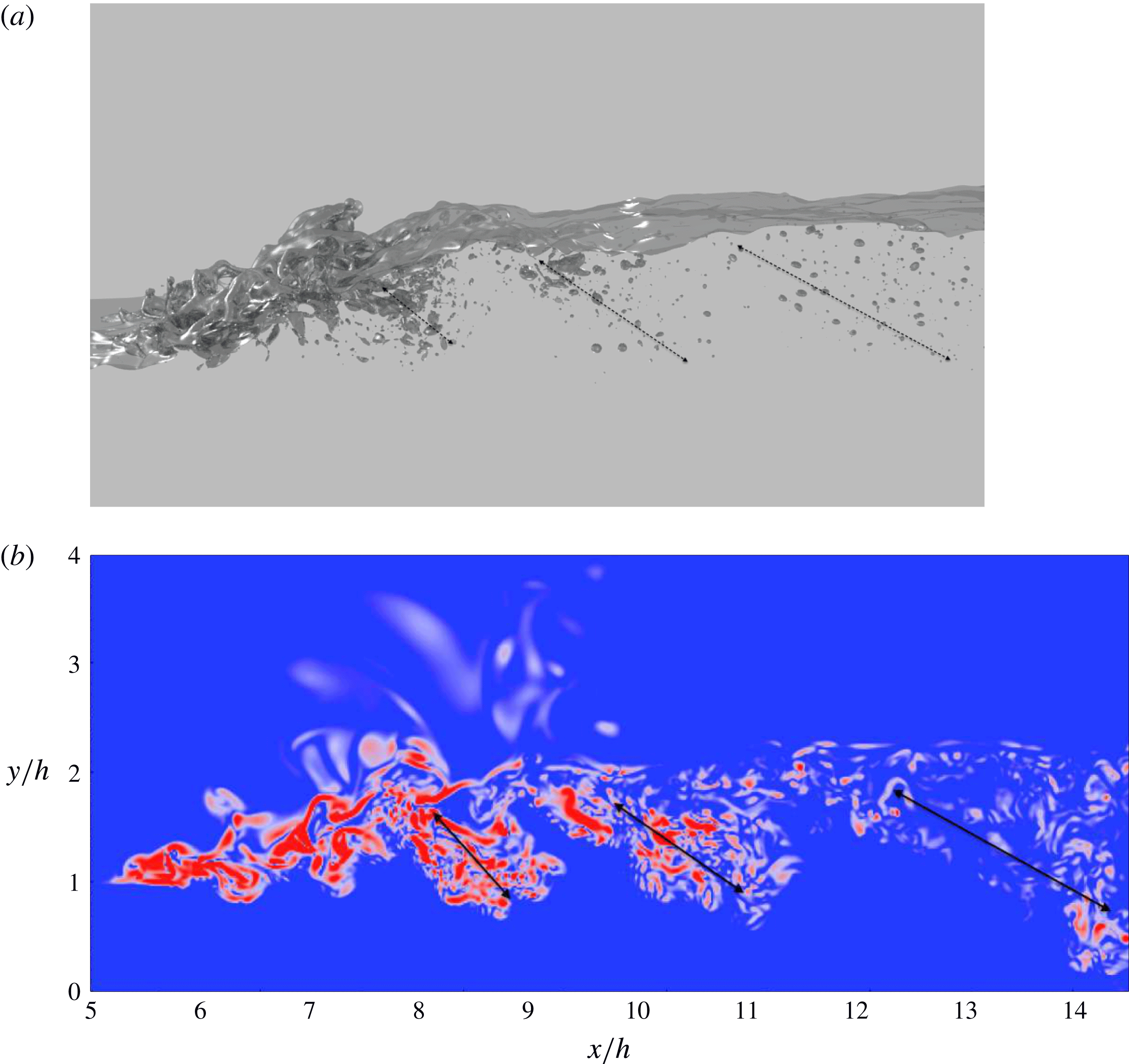
Bubbles and vorticity structures in the flow. The vorticity contour plot corresponds to the mid-plane in the spanwise direction, and both figures correspond to time
 $t=44.1\,h/U$
. (a) Bubble patches generated periodically and convected downstream with a non-dimensional frequency of
 $St=fh/U=0.141$
. (b) Vorticity magnitude contour shows coherent structures in the wake of the flow. Red colour indicates regions with a high vorticity magnitude.

Mok (Reference Mok2004) also experimentally measured the spectra of the surface fluctuations in hydraulic jumps with Froude numbers ranging from 1.4 to 3, and observed a dominant frequency for Froude numbers larger than
 $Fr=1.53$
. To further confirm the connection between the frequency peaks in the velocity spectra and the shedding phenomenon, we show in figure 17(b) the instantaneous vorticity contours. Spanwise vorticity packets are observed to be generated at the toe and advected downstream of the jump in a semiperiodic fashion. Passage of these vortices through the spectrum probes results in semiperiodic signatures predominantly in the vertical velocity measurements with a frequency that matches that of the shedding phenomenon. From analysis of the vertical velocity spectrum we determined the Strouhal number associated with the peak frequency to be
 $St=fh/U=0.14\pm 0.1$
. The Strouhal number based on the jump height,
 $1.37h$
, was computed to be
 $St=0.19\pm 0.1$
. While this Strouhal number is very close to the typically reported dimensionless frequency associated with the Kármán instability, the mechanism of vortex generation here is very different from that of the Kármán instability common to the wake of solid objects.
In the next section we show how vortex generation is correlated with air entrainment, and conclude that these coherent turbulent structures have a profound impact on bubble generation and transport in the wake of hydraulic jumps.
7 Air entrainment by coherent structures
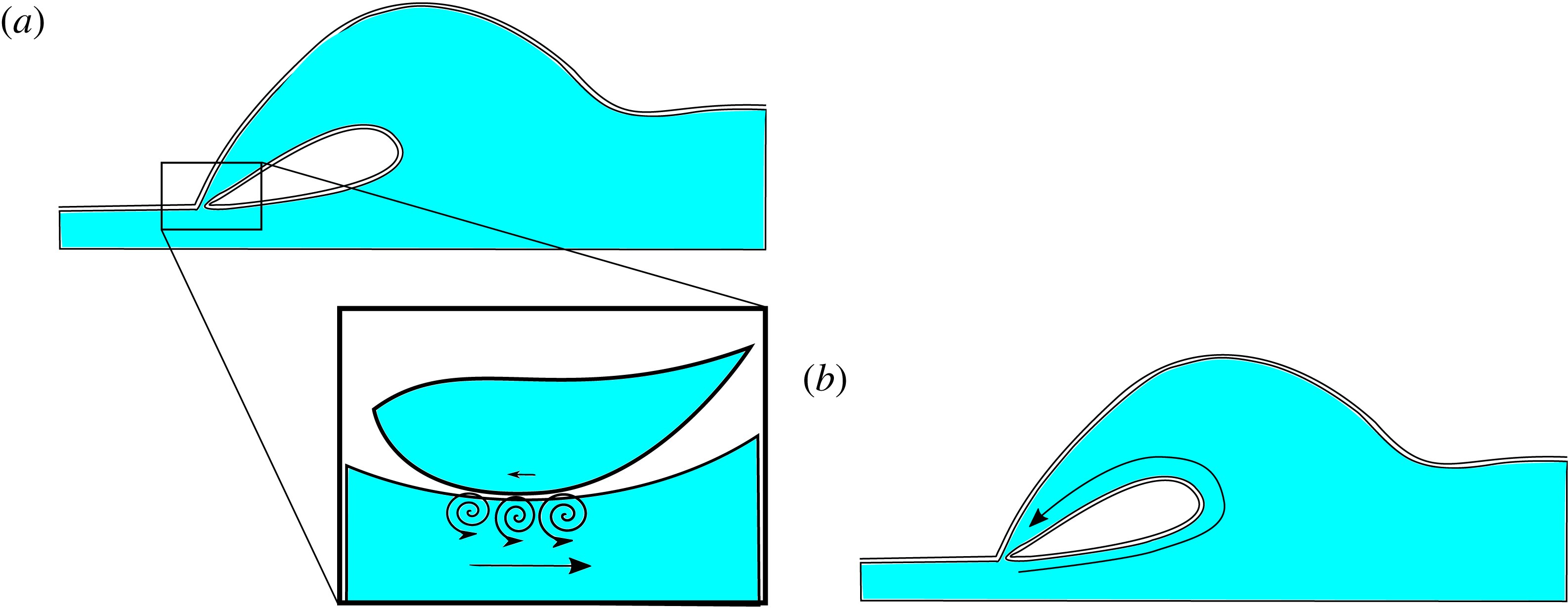
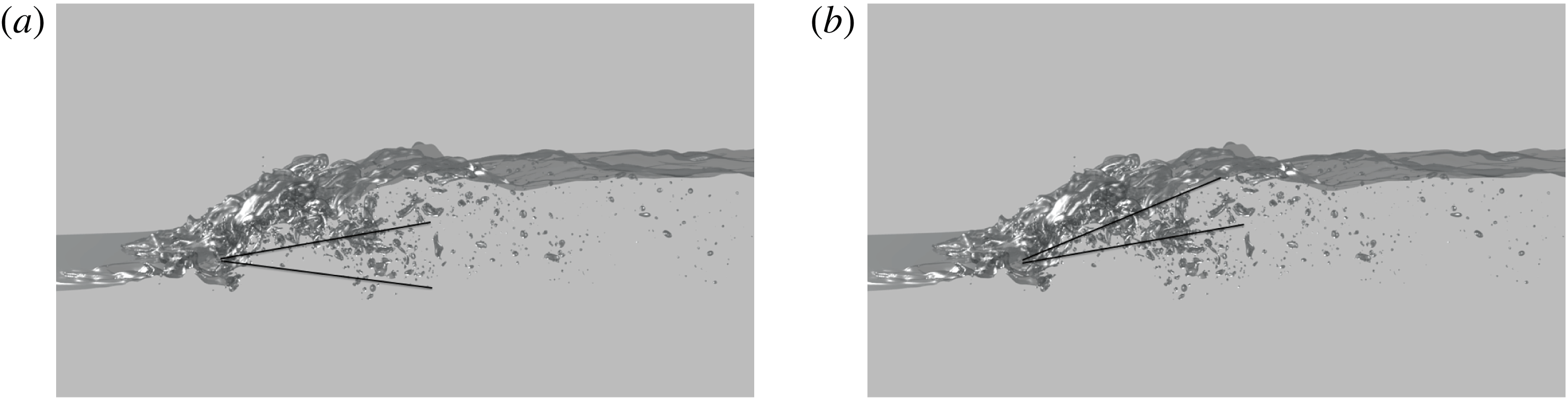
Air entrainment occurs mostly at the turbulent roller region of the hydraulic jumps as a result of wave breaking. Our observations suggest that the wave breaking in this problem is not a completely random phenomenon, but rather has a semiperiodic nature with a distinctive frequency. This periodic bubble generation can be visually observed in figure 17(a). Comparison of the coherent structures associated with the bubbles with the coherent structure of turbulent vortices in figure 17 suggests that there is a one-to-one correspondence between vortex ejection and air entrainment in the hydraulic jump. A quantitative analysis reveals that bubbles and vortices are generated at the same time with the same frequency. This one-to-one correspondence can be explained as follows: as schematically shown in figure 18, after air is engulfed by an overturning wave, vorticity is being injected into water during plunging events concurrent with the formation of vortex sheets associated with interface topological changes. In addition, the engulfed air zone has a net counterclockwise circulation, which is then diffused in the form of vorticity during topological changes associated with subsequent fragmentation processes. Hornung et al. (Reference Hornung, Willert and Turner1995) explain this vorticity injection connecting it with conservation of circulation before and after wave breaking events. The entrapped air and generated vorticity both advect downstream with the mean flow. Along this process, the entrapped air quickly fragments into smaller pieces and forms zones of bubble patches, indicated by arrows in figure 17(a).
Vorticity generation mechanisms as a result of topological changes in breaking waves. (a) Kinematic velocity jump at the impact points omits vortex sheets in the domain. (b) The entrained air cavity, which is generated as a result of an overturning breaking wave event, has a net circulation even in the inviscid limit. Further fragmentation of the air cavity generates more vorticity which will be diffused into the domain.

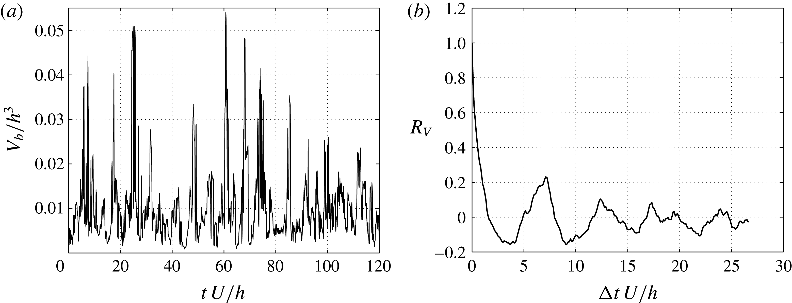
Bubble volume signal and its normalized autocorrelation for a region of
 $8.8<x/h<9.0$
: (a) bubble volume signal versus time; (b) auto-correlation of bubble volume signal. The autocorrelation plot shows a periodic behaviour of bubble patches passing through the domain. The non-dimensional Strouhal number associated with this phenomenon is
 $St=fh/U=0.141$
.

In order to measure the frequency of the generation of the bubble patches, we have computed the total volume of submerged air as a function of time in a fixed downstream window bounded by
 $8.8<x/h<9.0$
. Figure 19(a) shows the volume of bubbles in this interval as a function of non-dimensional time, denoted by
 $V_{b}(t)$
. We have chosen this interval in order to obtain a better signal of bubbles; very close to the toe the bubbles are not developed, the jump oscillates and the interaction with turbulence is too intense. As a result, the noise in the signal is significant. Further downstream the bubble patches are more diffused and the patch boundaries are harder to track. Figure 19(b) shows the autocorrelation of this signal defined as
 $$\begin{eqnarray}R_{V}({\rm\Delta}t)=\frac{\displaystyle \int _{0}^{\text{T}}V_{b}(t)V_{b}(t+{\rm\Delta}t)\,\text{d}t}{\displaystyle \int _{0}^{\text{T}}V_{b}(t)V_{b}(t)\,\text{d}t}.\end{eqnarray}$$
The first peak is at
 ${\rm\Delta}t=7.1\,h/U$
, which corresponds to the Strouhal number
 $St=0.141$
. This Strouhal number is very close to that of the peaks in the velocity energy spectra within our statistical errors. Therefore, the frequency of bubble-patch generation is the same as the frequency of the vortex-shedding phenomenon within statistical errors, and we conclude that breaking events at the toe of the jump are responsible for vortex generation, bubble-patch generation (present study) and interface fluctuations (Mok Reference Mok2004).
8 Summary
This report presents the first comprehensive study of a stationary turbulent hydraulic jump with dimensionless parameters:
 $Fr=2$
,
 $Re=11\,000$
and
 $We=1820$
, in which direct solution to the Navier–Stokes equation is employed to simulate this phenomenon. The simulation methodology employs a recently developed geometric VOF method (Le-Chenadec & Pitsch Reference Le-Chenadec and Pitsch2013) in order to track the phase interface. The combination of this numerical scheme, which has good mass conservation property and central difference schemes for momentum transport, allows for concurrent accurate prediction of bubbles and turbulence. Aside from comprehensive verification test cases, available experimental data are used for validation of our simulation. In comparing with experiments we match
 $We$
and
 $Fr$
as well as density ratios and viscosity ratios, and it is shown that Reynolds number (physically fluid viscosity) does not influence the presented DNS statistics. Specifically, reasonably good agreement is observed with experiments in void fraction measurements and interface length scale measurements (presented in the appendix A).
Reynolds-averaged mean velocity and fluctuations and Favre-averaged turbulent stress terms are computed. The velocity fluctuations are dominated by the streamwise direction at the toe and roller regions, but settle to close to isotropic condition after a few inlet heights downstream of the jump. The steepest rise of the mean interface spans streamwise distance of order two inlet heights, where the turbulence activity is strongest and is confined close to the interface. As one moves downstream of the jump, the vertical location where the velocity fluctuations, turbulence dissipation and Reynolds stresses peak asymptotes to approximately the average water heights between inflow and outflow. One-dimensional energy balance is investigated to elucidate energy transfer between different modes. While surface energy is found to play a negligible role in overall energy exchange processes, the kinetic energy was found to transfer to different modes in different orders. The peak of the exchange of kinetic energy to pressure work was found to precede that of the potential energy followed by the dissipation. In the beginning of the jump kinetic energy is mostly transferred to the pressure work, whereas far downstream the transfer is mostly between kinetic energy, potential energy and dissipation. Dissipation of energy was found to decay very slowly with streamwise distance, at its active phase up to order
 $10h$
downstream of the toe.
A 2-D turbulent kinetic energy dissipation term is also computed in the domain in order to gain insight into the interaction between the turbulence and bubble generation. The minimum Hinze scale diameter is found to be
 $D_{H}=0.05h$
(
 $2.8~\text{mm}$
). In the DNS results, a range of Hinze scales was observed due to variation of the turbulent kinetic energy dissipation in the domain.
Velocity energy spectra at three different streamwise locations in the jump were computed and a Kolmogorov-type spectrum with the slope of
 $-5/3$
was observed in the inertial range. In addition, coherent structures were found to have a paramount impact on turbulence, vorticity and bubble generation in the jump. A dominant frequency is distinguishable in the vertical velocity energy spectra which is related to the frequency of the rolling region at the front of the hydraulic jump. The generation of coherent vortex structures is observed and shown to be correlated with the bubble generation phenomenon. Bubble formation is not continuous in the flow, rather it has a semiperiodic nature. This hypothesis is examined by computing the void fraction downstream of the jump. The autocorrelation of this void fraction reveals a frequency which matches the dominant frequency of the velocity energy spectrum.
As demonstrated in this report, high-fidelity simulations complement experimental analyses of breaking waves by providing non-intrusive access to the detailed dynamical processes involved in wave breaking and air entrainment over fine spatio-temporal resolutions. However, there are currently two barriers against detailed matching between DNS and physical experiments: (a) computational cost of DNS at realistic Reynolds numbers is prohibitively expensive and (b) in physical experiments, it is not possible to keep
 $Fr$
fixed and tune
 $Re$
and
 $We$
independently. The latter is possible computationally, and our study presents these results. One possible extension of the presented analysis would be to expand the explored regime to a wide range in the parameter space. With improved numerical algorithms and as the available computing power increases, it will be possible to resolve flow features over more energetic waves and simulate hydraulic jumps with larger
 $Fr$
and
 $We$
. Additionally, the presented hypothesis of weak sensitivity of air entrainment on the Reynolds number can be examined over a wider range of
 $Re$
.
Acknowledgements
We thank the anonymous referee no. 1 for various helpful comments including remarks on effects of Reynolds number on hydraulic jumps in physical experiments and pointing us to multiple experimental papers. This work was supported by the Office of Naval Research under grant number N000141110030 monitored by Drs P. Purtell, K.-H. Kim and T. Fu.
Supplementary material
Supplementary material is available at http://dx.doi.org/10.1017/jfm.2016.230.
Appendix A. Comparison with experimental measurements
While the employed numerical algorithm is extensively verified and validated in Le-Chenadec & Pitsch (Reference Le-Chenadec and Pitsch2013), here we present a comparison against available data from experiments in the specific regime of our simulation. To this end, we first present the void fraction of air in comparison to the results of Murzyn et al. (Reference Murzyn, Mouaze and Chaplin2005), and then we investigate the interface length scale in comparison to the measurements of Murzyn et al. (Reference Murzyn, Mouaze and Chaplin2007).
A.1 Air entrainment
Murzyn et al. (Reference Murzyn, Mouaze and Chaplin2005) have distinguished two separate regions downstream of the toe of the hydraulic jump. These regions have different characteristics in bubble generation mechanisms and void fraction distribution. Figure 20 shows these two regions. In the lower region, the interaction of the interface is minimal and bubbles generated at the toe are convected and diffused downstream in the turbulent shear layer. The upper region is located in the roll-up region of the flow and experiences more interactions with the interface.
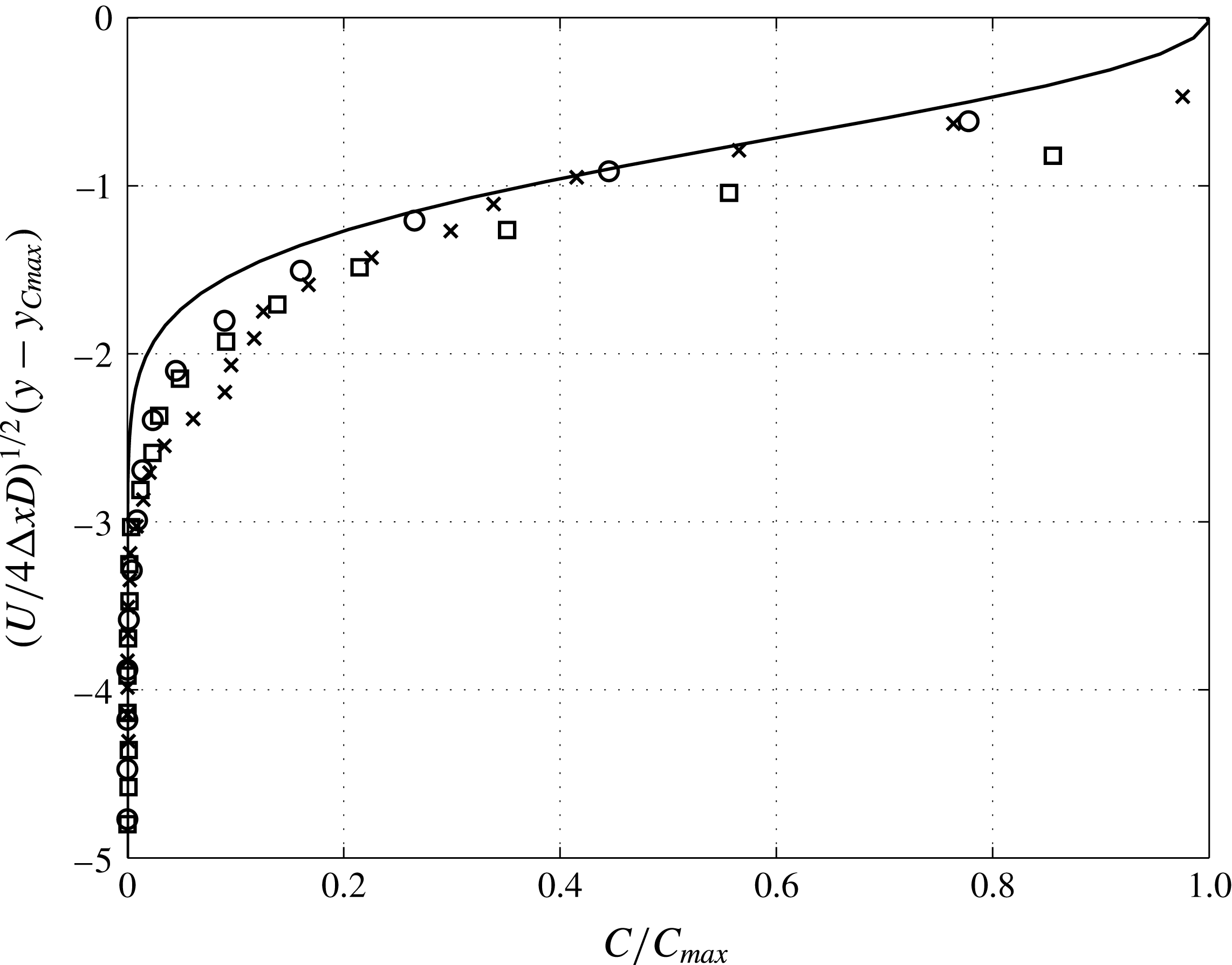
Chanson (Reference Chanson1996) has argued that bubbles in the lower region of a hydraulic jump undergo an advection–diffusion process, and therefore the void fraction can be fit to a Gaussian profile. Murzyn et al. (Reference Murzyn, Mouaze and Chaplin2005) also confirmed this result and showed that the void fraction obeys a Gaussian profile,
 $$\begin{eqnarray}C=C_{max}\exp \left(-\frac{1}{4}\frac{U}{D}\frac{(y-y_{Cmax})^{2}}{{\rm\Delta}x}\right),\end{eqnarray}$$
where
 $C$
is the void fraction, and
 $C_{max}$
,
 $D$
,
 $y_{Cmax}$
are the parameters representing maximum void fraction, effective diffusivity and vertical location of the maximum void fraction, respectively.
 ${\rm\Delta}x=x-x_{t}$
represents the streamwise coordinate measured from the toe of the jump,
 $x_{t}$
, which is not defined accurately in the experiment. We found that the value of
 $x_{t}/h=6.1$
gives the best void fraction comparison with the values reported in the experiment.
Two regions of air entrainment in the hydraulic jump: (a) lower region and (b) upper region.

Simulation results of void fraction in the lower region of the hydraulic jump. The solid line represents the experimental fit by Murzyn et al. (Reference Murzyn, Mouaze and Chaplin2005). Symbols represent results from current simulation at downstream locations,
 ${\rm\Delta}x/h=0.85$
(○), 1.70 (▫) and 2.54 (
 $\times$
).

In their experiments, Murzyn et al. (Reference Murzyn, Mouaze and Chaplin2005) report the values for
 $C_{max}(x)$
,
 $y_{Cmax}/h$
and
 $D/Uh$
. From the experimental study we have used
 $C_{max}=4.391\times 10^{-2},1.147\times 10^{-2},1.170\times 10^{-2}$
and
 $y_{Cmax}/h=1.073,1.061,1.162$
and
 $D/Uh=3.26\times 10^{-3},2.94\times 10^{-3},3.76\times 10^{-3}$
, respectively for streamwise locations
 ${\rm\Delta}x/h=0.85,1.70,2.54$
. Using these parameters, figure 21 presents the ensemble-averaged void fraction data in the lower region of the jump from our simulation and contrasts results against the experimental fit. Given that none of the parameters are retuned (i.e.
 $C_{max}$
,
 $D$
and
 $y_{Cmax}$
are all from the experiment), the match between the two data sets is remarkable. The discrepancies can be attributed to the fact that the experiment involved a thin boundary layer below the jump, which was intentionally avoided in our simulation. According to the experiment, the boundary layer thickness at the toe of the jump is approximated to be
 ${\it\delta}/h=0.18$
. This boundary layer thickness would translate to a displacement thickness of approximately
 ${\it\delta}^{\ast }={\it\delta}/3$
, which, in terms of the variable of the vertical axis of figure 21, is between 0.3 to 0.6 depending on the value of
 ${\rm\Delta}x$
. The mismatch between the simulation and experimental data is within this error, and can be explained by the thin boundary layer at the bottom wall in the experiment.
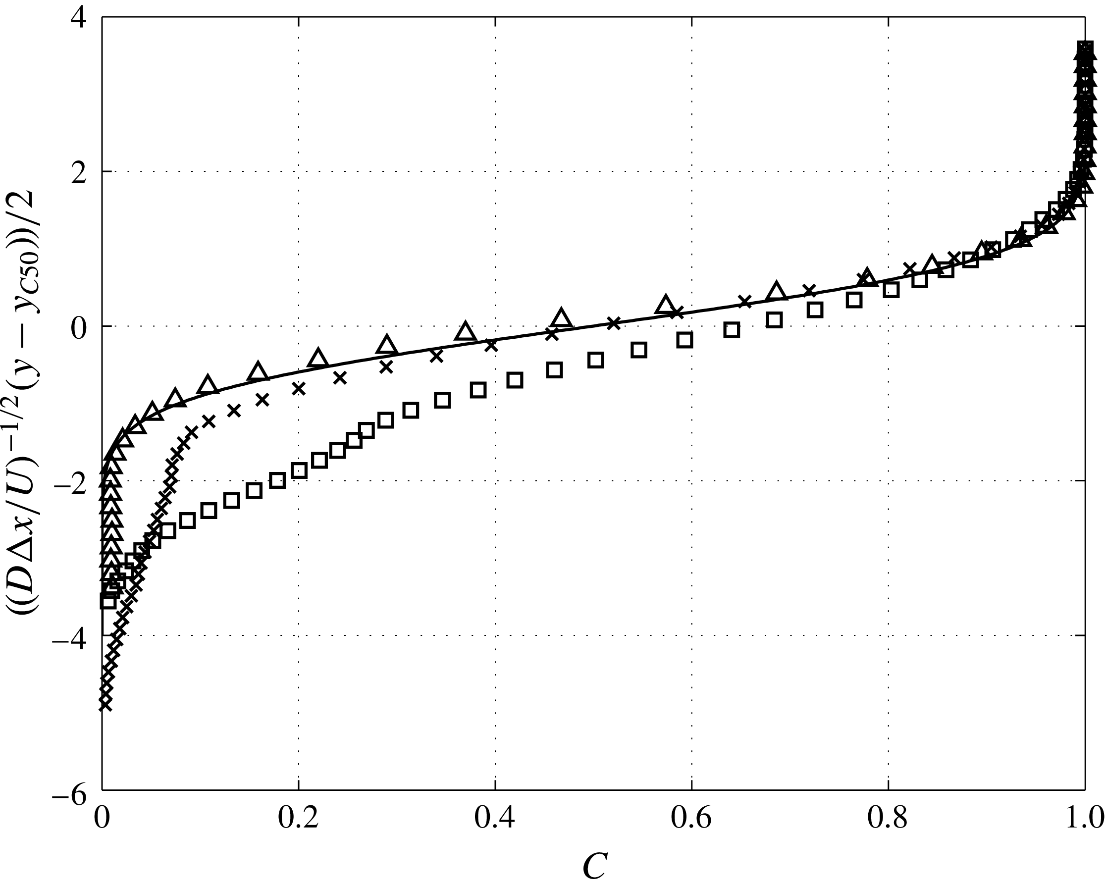
According to Murzyn et al. (Reference Murzyn, Mouaze and Chaplin2005), the upper region of the jump is influenced by the interfacial air exchange. A reasonable fit is proposed by Brattberg et al. (Reference Brattberg, Toombes and Chanson1998) in the form of
 $$\begin{eqnarray}C=\frac{1}{2}\left[1+\text{erf}\left(\frac{y-y_{C50}}{2\sqrt{D{\rm\Delta}x/U}}\right)\right],\end{eqnarray}$$
where
 $y_{C50}$
is the vertical position for which the void fraction equals
 $0.5$
. The void fraction is not normalized in this case since its maximum is one in the air side. Similar to the lower region, the experiment of Murzyn et al. (Reference Murzyn, Mouaze and Chaplin2005) reports the values for
 $y_{C50}$
and
 $D/Uh$
. According to the experiment, we have used
 $y_{C50}/h=1.77,2,2.15$
and
 $D/Uh=8.53\times 10^{-3},4.84\times 10^{-3},1.93\times 10^{-3}$
, respectively for streamwise locations
 ${\rm\Delta}x/h=1.70,2.54,4.24$
. Figure 22 shows the ensemble-averaged void fraction in the upper region of the jump from our simulation in comparison to the experimental fit. Similar to the lower region of the jump, comparison to the experimental results is reasonably good. The deviation of the void fraction from (A 2) is also observed in the experiment for the region of
 $C<0.4$
, showing that (A 2) is more accurate for larger values of void fraction and closer to the free surface.
Time- and spanwise-averaged simulation results for void fraction in the upper region of the hydraulic jump. The solid line represents the experimental fit by Murzyn et al. (Reference Murzyn, Mouaze and Chaplin2005). Symbols represent results from current simulation at downstream locations,
 ${\rm\Delta}x/h=1.70$
(▫), 2.54 (
 $\times$
) and 4.24 (
 $\triangle$
).

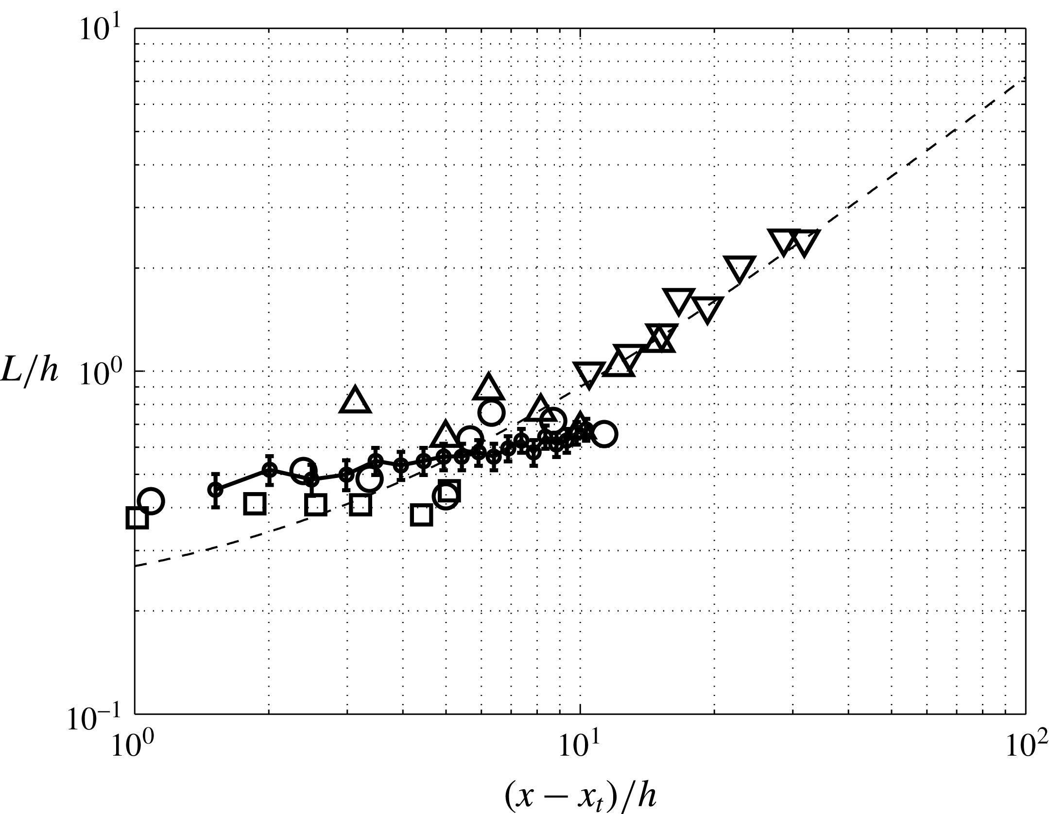
Interface length scale validation of the simulation. (●) Integral length scale computed from the simulation. The statistical error for the calculations is within
 $\pm 10\,\%$
. The symbols denote (▫)
 $Fr=2$
, (○)
 $Fr=2.4$
, (▵)
 $Fr=3.7$
, (▿)
 $Fr=4.8$
, (– –) experimental fit (Murzyn et al.
Reference Murzyn, Mouaze and Chaplin2007).

A.2 Interface length scale
Interface length scale is another quantity that Murzyn et al. (Reference Murzyn, Mouaze and Chaplin2007) have studied. They define the interface length scale,
 $L$
, at a particular position of the hydraulic jump as the integral under the autocorrelation curve
 $R(r)$
, of the electric signal
 $s$
. This signal is proportional to the water depth of the immersed probe and measures the instantaneous water height. The definition of the correlation function and the interface length scale is as follows:
 $$\begin{eqnarray}\displaystyle & \displaystyle R(r)=\frac{\overline{s_{A}\cdot s_{B}}}{\sqrt{\overline{s_{A}^{2}}}\sqrt{\overline{s_{B}^{2}}}}, & \displaystyle\end{eqnarray}$$
 $$\begin{eqnarray}\displaystyle & \displaystyle L=\int _{0}^{r_{max}}R(r)\,\text{d}r, & \displaystyle\end{eqnarray}$$
where
 $r$
is the distance between
 $A$
and
 $B$
and
 $r_{max}$
is the distance where
 $R(r_{max})\approx 0$
.
In the simulations we have considered the level set variable, which by definition is the distance of each point to the interface (it is positive inside water and negative outside), to compute the integral length scale. The interface length scale is thus defined as the integral under the autocorrelation curve of the level set signal, up to
 $5\,\%$
correlation. Figure 23 shows a comparison between the simulation results and the experiment. It can be seen that the interface length scale increases with the streamwise position and the predicted interface length from our simulation compares well with the experimental data.
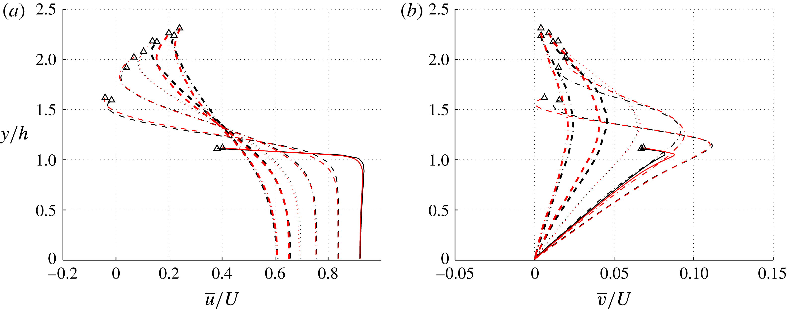
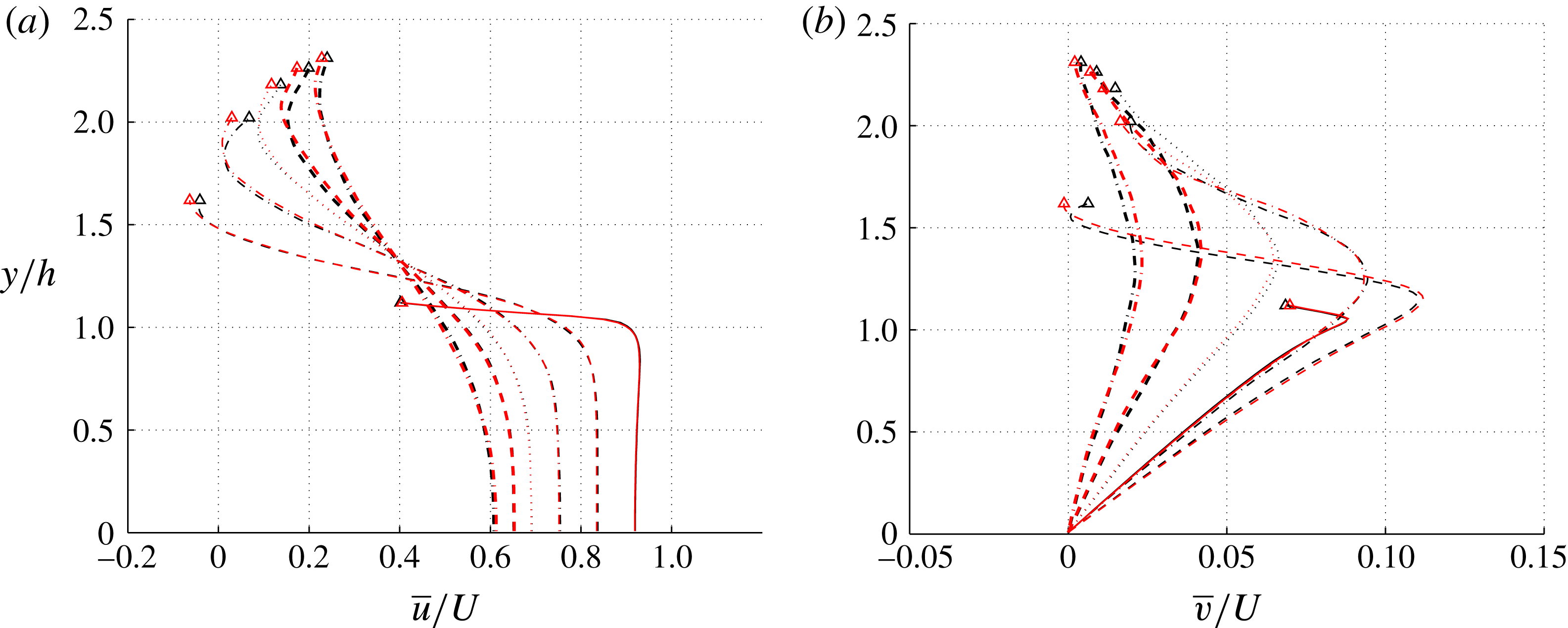
Mean velocity profiles for different streamwise positions and two different meshes: red, fine mesh; black, coarse mesh;
 $(x-x_{t})/h=0$
(——), 1.0 (– –), 2.0 (— ⋅ —), 3.0 (
 $\cdots \cdots$
), 4.0 (– –) and 6.0 (— ⋅ —). The symbols show the position of
 $\overline{VF}=0.5$
.

Appendix B. Grid refinement study and statistical convergence
As discussed in § 2.4, we have performed the calculations on two grids. The fine calculation, of which we presented the turbulence results, in this chapter, has twice the grid size in each direction compared to the coarse calculation. The aim of this section is to present the mean velocity and the energy exchange data for these two calculations and test the convergence of the results.
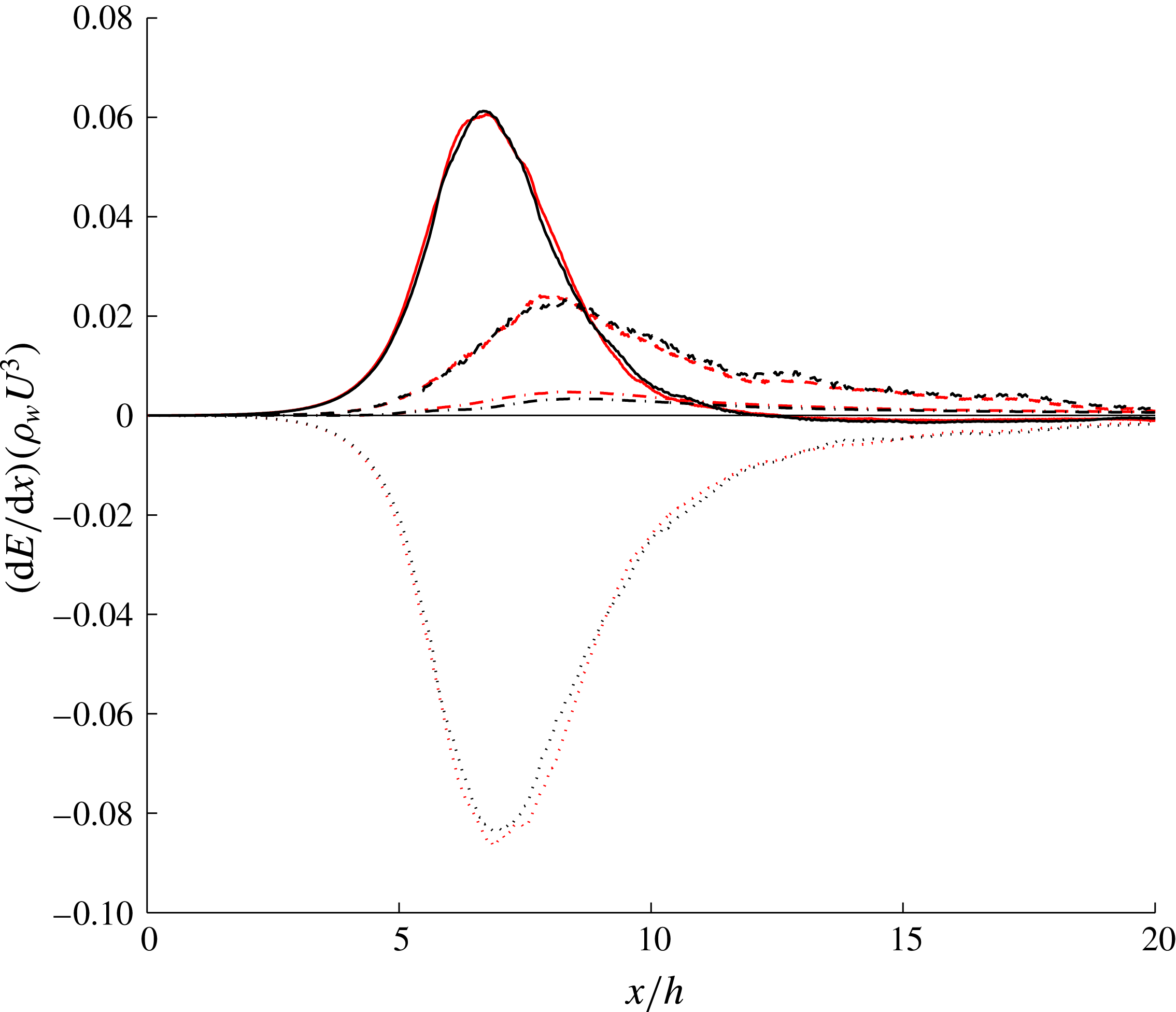
Figure 24 shows the convergence of the mean velocity profiles between the coarse and fine meshes. We can see a good agreement between the two calculations in the water region. We have also computed the 1-D energy exchange terms which were introduced in § 4 shown in figure 25. The kinetic energy flux, potential energy flux and pressure work show convergence between the two calculations.
Transfer of kinetic energy to other forms of energy as a function of streamwise location. The plots represent exchange rates due to kinetic energy (
 $\cdots \cdots$
), potential energy (– –), pressure work (——) and dissipation (— ⋅ —), for: red, fine mesh, and black, coarse mesh.

Mean velocity profiles for different streamwise positions and two different Reynolds numbers: red,
 $Re=5500$
; black,
 $Re=11\,000$
;
 $(x-x_{t})/h=0$
(——), 1.0 (– –), 2.0 (— ⋅ —), 3.0 (
 $\cdots \cdots$
), 4.0 (– –) and 6.0 (— ⋅ —). The symbols show the position of
 $\overline{VF}=0.5$
.

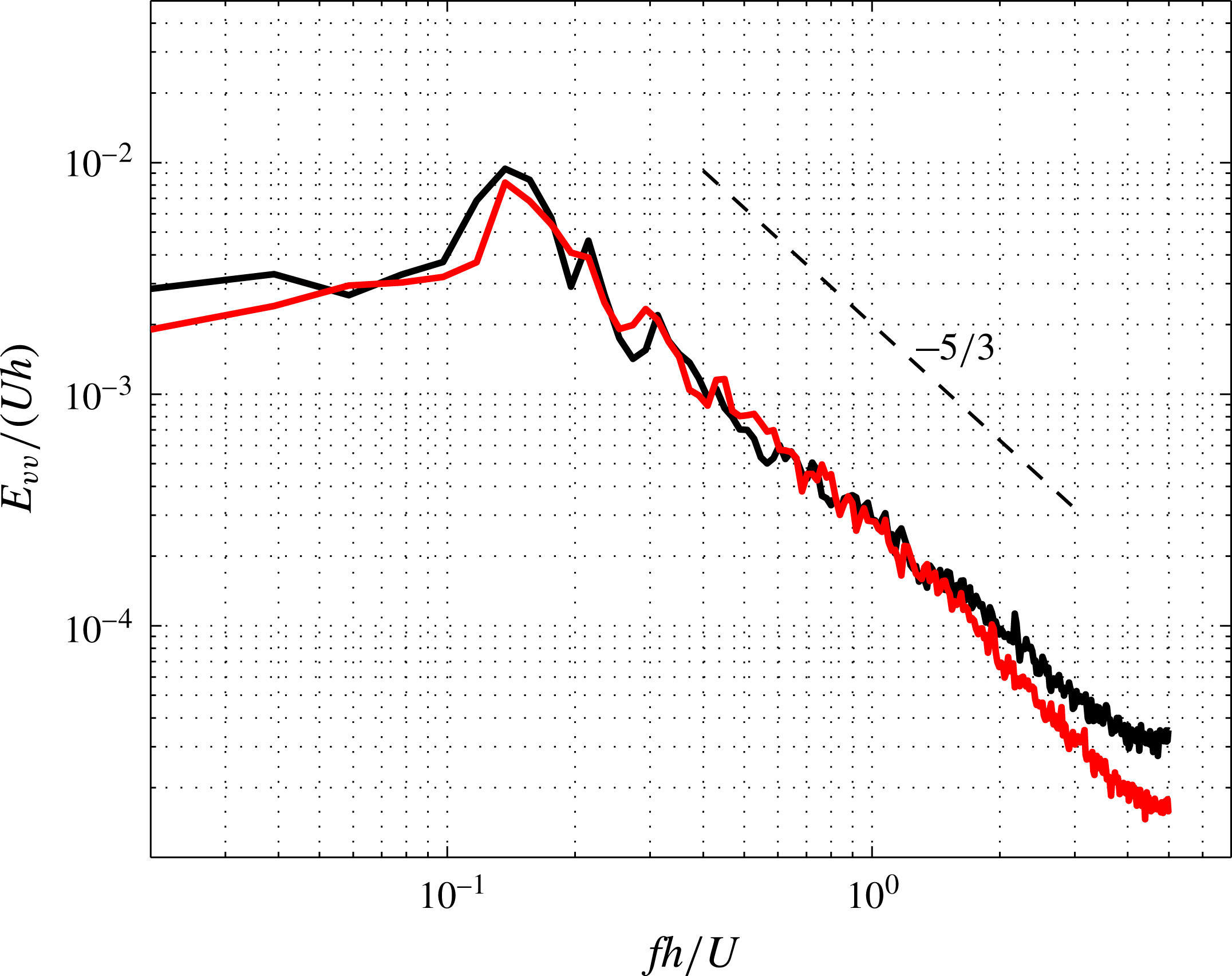
Energy spectrum for vertical velocity component at
 $(x-x_{t})/h=2.0$
: red,
 $Re=5500$
; black,
 $Re=11\,000$
;

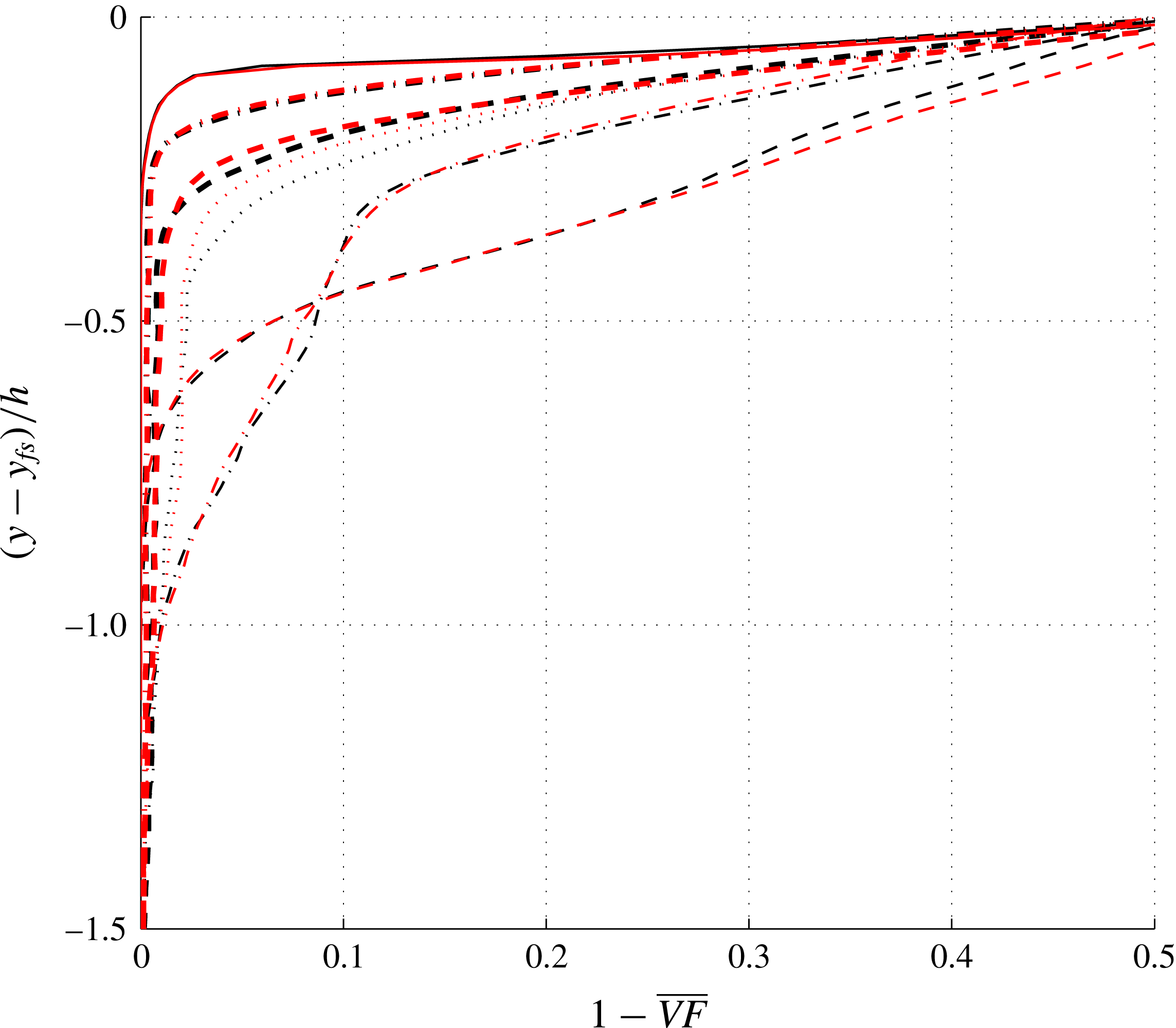
Cross-sectional profiles of mean void fraction: red,
 $Re=5500$
; black,
 $Re=11\,000$
;
 $(x-x_{t})/h=0$
(——), 1.0 (– –), 2.0 (— ⋅ —), 3.0 (
 $\cdots \cdots$
), 4.0 (– –) and 6.0 (— ⋅ —). Here
 $y_{fs}$
is the vertical location of the interface at the corresponding
 $x/h$
.

Appendix C. Reynolds number effects
In this appendix we provide a comparison between two sets of simulations with different inlet Reynolds numbers. The nominal case which its results are discussed in this paper in detail (
 $Fr=2.0$
,
 $We=1820$
,
 $Re=11\,000$
) is compared with simulation results of a hydraulic jump with
 $Fr=2.0$
,
 $We=1820$
and
 $Re=5500$
. The Reynolds number is reduced in the latter simulation by doubling the viscosity of water and air so that the viscosity ratio is still the same as the nominal case. All the other parameters of the two simulations are the same.
In figures 26 and 27 we compare the mean velocity profiles at different streamwise locations of the jump and the energy spectrum associated with the vertical velocity component at
 $(x-x_{t})/h=2.0$
, respectively. Figure 26 shows that the mean velocity profiles in the water is not sensitive to the Reynolds number. Furthermore, figure 27 illustrates that the energy spectra of the two cases do not differ significantly. A peak with a distinctive frequency is observed at the same frequency for the two cases. These peaks which their significance is discussed in § 7 show that the processes of bubble generation and vorticity generation are similar between the two cases, and Reynolds number does not affect these phenomena significantly. The major difference in the spectra is in low-energy high-wavenumber regions, where the case with higher Reynolds number has higher energy. This difference is expected given that smaller viscosity allows cascade of turbulence to smaller feature sizes.
Figure 28 compare void fraction between the nominal hydraulic jump and the one with half the Reynolds number. Void fraction profiles are compared at different streamwise locations between the two simulations in figure 28. This figure shows that the effect of the inflow Reynolds number is not significant for air entrainment process.
Profiles of the Reynolds stresses, scaled with fitted similarity variables. For all plots the virtual streamwise origin is set to
 $x_{o}/h=4$
. The parameters
 ${\it\alpha}$
and
 ${\it\beta}$
are: (a)
 ${\it\alpha}=-2.2$
,
 ${\it\beta}=0.5$
, for
 $7.8<x/h<12$
; (b)
 ${\it\alpha}=-1.5$
,
 ${\it\beta}=0.5$
, for
 $7.8<x/h<10$
; (c)
 ${\it\alpha}=-1.65$
,
 ${\it\beta}=0.5$
, for
 $7.8<x/h<12$
.

Appendix D. On the self-similarity of turbulence statistics
Turbulence Reynolds stresses as defined in (3.4) and plotted in figure 11 show spatial variability. In this section we investigate whether variations of these profiles exhibits a self-similar behaviour. This investigation is motivated by the study of Dimotakis (Reference Dimotakis1986) who reported self-similar growth of shear layers between fluid streams with different densities. These authors reported linear growth of shear layer thickness with streamwise distance. Our investigations indicate that similar trends do not hold for the case of the studied hydraulic jump. Nevertheless, we report a fit that could best collapse our data. We explore self-similar profiles in the following form:
 $$\begin{eqnarray}\frac{\widetilde{{\it\tau}}_{ij}}{({\it\rho}_{w}U^{2})(x/h-x_{o}/h)^{{\it\alpha}}}=f\left(\frac{y/h-y_{max}/h}{(x/h-x_{o}/h)^{{\it\beta}}}\right),\end{eqnarray}$$
where
 $\widetilde{{\it\tau}}_{ij}$
is the component of the Reynolds stress, and
 $y$
is the vertical coordinate.
 $y_{max}(x)$
is the vertical coordinate of maximum turbulent shear stress at each streamwise section.
 $x_{o}$
is the streamwise location of the similarity coordinate origin.
 ${\it\alpha}$
and
 ${\it\beta}$
together with
 $x_{o}$
are the similarity parameters that are obtained by fitting. Figure 29 shows the Reynolds stress profile with best fitting scenarios. Based on these data, we conclude that the self-similarities reported by Dimotakis (Reference Dimotakis1986) do not hold for the case of a hydraulic jump. For example, the fitted values for
 ${\it\beta}$
are close to
 $0.5$
which is far from the linear growth demonstrated for shear layers. Additionally, given the variability of the plots, even after rescaling, we conclude that the Reynolds stress profiles are hardly self-similar when it comes to turbulent hydraulic jumps.