1. Introduction
In financial risk management, loss distribution modeling is an integral component in consequential decision-making processes, ranging from determining capital adequacy to pricing and structuring reinsurance and insurance contracts or policies, and assessing solvency under regulatory and internal risk requirements for an institution or writer. It enables accurate estimation of potential losses, which may be frequent or rare, and ensures that insurance and financial institutions are strong during periods of uncertainty. Classical single-component statistical models, including Gamma, Weibull, and lognormal, as well as other distributions, have been effective due to their analytical tractability and capacity to model non-negative and skewed datasets. However, when applied to fit empirical loss data, these models fail, particularly for those with rare extreme events that have significant financial impacts, such as catastrophe insurance and other high-risk areas. These empirical loss data typically exhibit a dual behavior: a high-frequency component of small to moderate losses (especially the body of the distribution), with a long, heavy tail of large, rare, or infrequent losses. This bi-modality is problematic for classical unimodal distributions, however, as they cannot simultaneously fit both the body and the tail of the distribution to a high degree of accuracy. Whenever a single parametric distribution is stretched to fit both regions, it tends to compromise between the fit to the body and the fidelity in the tail. This inconsistency can lead to a systematic underestimation of tail risks, resulting in poor reinsurance layer pricing, economic capital misallocation, and increased risk of solvency breach under stress conditions.
To address this deficiency, Cooray and Ananda (Reference Cooray and Ananda2005) proposed the first composite model ever to simulate the dual nature of insurance data. This model paved the way for more innovative and advanced models in the actuarial and financial risk management field. The fundamental concept of their model was to employ a lognormal distribution for modeling the frequent small to medium losses and the Pareto distribution for the less frequent but considerably large claims. However, it is criticized by Scollnik (Reference Scollnik2007), who called it a priori known weighted mixture of a two-component distribution rather than a composite model and proposed his own composite lognormal–Pareto model with unrestricted weights for the components, which is more flexible due to the tuning of different ratios of two-component distributions in the composite model. Later, Pigeon and Denuit (Reference Pigeon and Denuit2011) extended his work when they allowed the varying threshold amidst the observations rather than being fixed as it was in Scollnik’s model. Aligning with this extension, they used the Gamma-distributed and lognormal-distributed distributions as threshold distributions in modeling. Nadarajah and Abu Bakar (Reference Nadarajah and Abu Bakar2014) observed, while modeling the classical Danish Fire Insurance dataset, that their proposed new composite lognormal–Burr model outperformed the then-existing composite lognormal–Pareto family distribution. Ciumara (Reference Ciumara2006), working on a similar kind of idea, introduced a model of a composite of Weibull for modeling frequent small to moderate losses, while Pareto for the large losses, which are less frequent. However, the model is criticized by Scollnik and Sun (Reference Scollnik and Sun2012) for having a fixed set of weights for the components, and they introduce their composite model with unrestricted or varying weights using the new Weibull-led family of composite distributions.
Abu Bakar et al. (Reference Abu Bakar, Hamzah, Maghsoudi and Nadarajah2014) then introduced a series of seven new composite distributions by keeping the Weibull as the body of the distribution and the tail from the transformed beta distribution family (which includes Pareto, Burr, Logistic, and Paralogistics, and their inverse forms as Inverse Burr, Inverse Pareto, and Inverse Paralogistic), and the results of their study revealed that the Weibull-led body–tail combination outperformed any other existing composite models in the literature. Thereafter, this framework is further extended by Miljkovic and Grün (Reference Miljkovic and Grün2016), who conduct a thorough analysis using
 $16 \times 16$
distinct parametric distributions for the combinations of body and tail in the composite distribution. A decision about the superiority of the models is made using the Bayesian Information Criterion (BIC). The study revealed that for the top 20 combinations, none of the distributions had a lognormal distribution as the body of the distribution. Additionally, it was found that neither the Pareto nor the generalized Pareto distributions (GPDs) were included in the top 20 combinations in any manner. Asgharzadeh et al. (Reference Asgharzadeh, Nadarajah and Sharafi2017) introduced a generalized inverse Lindley distribution for modeling the losses, and their results indicated that it is better than classical heavy-tailed distributions but fails to compete against composite distributions. Punzo et al. (Reference Punzo, Bagnato and Maruotti2017) worked on compound models for modeling losses, whose resultant models are more flexible than unimodal two-parameter distributions due to the addition of extra parameters.
Calderin-Ojeda and Kwok (Reference Calderin-Ojeda and Kwok2016) employed an innovative approach to form a composite model by utilizing the modal value of the component distributions as the transition/splice point. They developed two new Weibull–Stoppa and lognormal–Stoppa composite models, in which Weibull–Stoppa had the best performance (at that time) against any other composite model for the classical Danish Fire Insurance dataset. This new approach has been helpful in replacing the continuity and differentiability conditions for complex modeling, as it is easier to match modal values. Additionally, it will be beneficial for parameter estimation due to the closed-form solution. Jones and Pewsey (Reference Jones and Pewsey2009), Scollnik and Sun (Reference Scollnik and Sun2012), and related studies have developed smooth splicing and smooth transition composite models by explicitly enforcing continuity or differentiability of the density or distribution function at a fixed splice point. Empirical results show that such constraints can improve global fit and mathematical regularity relative to abrupt threshold-based composite models. However, Bader et al. (Reference Bader, Yan and Zhang2018) supported the sensitivity concerns noted by Coles (Reference Coles2001), and Beirlant et al. (Reference Beirlant, Goegebeur, Segers and Teugels2004) states that inference can be sensitive to the choice and estimation of threshold parameters, with significant effects on parameter stability and tail-related risk measures. These findings suggest the need for alternative composite constructions that regulate the transition between the body and tail without relying on hard splice constraints, thereby motivating hazard-based blending frameworks.
The study is inspired by recent work of Grün and Miljkovic (Reference Grün and Miljkovic2019), where they found that a finite mixture developed using either Burr or Inverse Burr fit the classical Danish fire losses best, and later they also extended their study by taking a
 $16\times 16$
combination of parametric distributions in the form of the body and tail of the composite distributions. The study is also inspired by the need for a seamless transition between these two regimes (head and tail of the composite), which is not captured in recent composite formation using probability density function (PDF) and cumulative density function blends.
Recent advancements in parametric modeling of Danish fire insurance loss data include the tuning-based and iterated distribution frameworks proposed by Mohammad and Cooray (Reference Mohammad and Cooray2025a,b), which explore alternative strategies for tail-risk estimation through controlled parameter adjustment and flexible distributional construction. These approaches have explicit emphasis on tail behavior under settings where extreme-quantile calibration is a primary objective, complementing likelihood-based inference in the heavy-tailed actuarial models. Their findings highlights the practical importance of carefully balancing the global goodness-of-fit with the tail-specific considerations when modeling an insurance loss data.
The novelty of this study lies in three key aspects. First, a hazard-blend composite framework is proposed that ensures a smooth and differentiable transition between the body and tail distributions, thereby avoiding the discontinuities which are common in traditional spliced models. Second, the Bayesian and frequentist estimation methods are compared, to focus on the effects of the prior specification (weak vs. empirical) which influences the tail inference and solvency metrics. Third, a comparative analysis of empirical and model-based capital requirements and reinsurance pricing is presented, which provides the valuable insights into the practical implications for the contract design and solvency regulation. By combining the methodological rigor with the regulatory and actuarial relevance, these contributions strengthen the literature on composite loss modeling.
The paper is properly structured as follows: A brief description of the methodology, including the model specification, estimation approaches, risk & solvency measure, reinsurance pricing and payouts, and model selection criteria is provided in Section 2. Following this, Section 3 presents the analysis of goodness-of-fit, risk & solvency measures, and reinsurance pricing and payouts, for the simulated dataset. Section 4 provides an analysis of the empirical data from the Danish Fire Insurance dataset, including the results. Following this, there are Sections 5 and 6, which conclude the study with a discussion and conclusion, as well as an outline of the future scope of the study.
2. Methodology
This section outlines the methodological framework developed for constructing, estimating, and validating the proposed hazard-blend composite model. It begins with the model specification, followed by estimation techniques, risk and solvency measures, reinsurance pricing strategies, and model evaluation criteria.
2.1. Model specification
We begin with a non-negative random variable
 $ \textit{X} \in \mathbb{R}_+ $
representing insurance losses. Rather than stitching distributions using densities or survival functions, we use hazard rates since convex combinations of hazard rates yields a valid distribution and uniquely determine it via the cumulative hazard.
A hazard-rate blending approach is adopted, introduced by Lawless (Reference Lawless2002), to ensure a smooth and valid composite distribution. In the literature, composite models such as lognormal–Pareto blends of Cooray and Ananda (Reference Cooray and Ananda2005), Scollnik (Reference Scollnik2007), and random threshold composites of Pigeon and Denuit (Reference Pigeon and Denuit2011) are well established, as are mixture methods by Miljkovic and Grün (Reference Miljkovic and Grün2016) and Abu Bakar et al. (Reference Abu Bakar, Nadarajah and Adzhar2017). In particular, Grün and Miljkovic (Reference Grün and Miljkovic2019) presents a computational framework for rich composite model calibration.
Let
 $F_B(x)$
and
 $F_T(x)$
be the cumulative distribution functions (CDFs) of the body and tail distributions, respectively, defined on the domain
 $x \in \mathbb{R}_+$
. Let their corresponding PDFs be
 $f_B(x)$
and
 $f_T(x)$
, and their survival functions be
 $S_B(x) = 1 - F_B(x)$
and
 $S_T(x) = 1 - F_T(x)$
, then the corresponding hazard rates are defined as:
 \begin{equation} h_B(x) = \frac{f_B(x)}{S_B(x)}, \quad h_T(x) = \frac{f_T(x)}{S_T(x)}. \end{equation}
A logistic blending weight function is used for a smooth transition between the two distributions:
 \begin{equation} w(x) = \frac{1}{1 + e^{-k(x - \tau)}}, \end{equation}
where
 $\tau \gt 0$
is the transition point, and
 $k \gt 0$
controls the steepness of the transition.
The composite hazard rate h(x) is then defined as a convex combination:
 \begin{equation} h(x) = (1 - w(x)) h_B(x) + w(x) h_T(x). \end{equation}
This guarantees smoothness because the logistic weight is infinitely differentiable, and hence h(x) and all induced distributional quantities (CDF, PDF, and survival) are also smooth.
The composite survival function is given as:
 \begin{equation} S(x) = \exp\!\left(-\int_0^x \left[(1 - w(u)) h_B(u) + w(u) h_T(u)\right] du\right)\!. \end{equation}
The logistic weight is adopted as it satisfies key requirements of hazard-based blending, namely boundedness in [0,1], smoothness, numerical stability, and interpretability through the transition location
 $\tau$
and the steepness parameter k. Alternative specifications, including probit, hyperbolic tangent, Cauchy, and softmax weights, were also examined; detailed comparative results are reported in Appendix A.1. These alternatives exhibit a similar qualitative behavior, with only marginal differences in the predictive performance. Consequently, the logistic weight is retained as a stable and interpretable choice for smooth hazard blending.
Unlike smooth splicing approaches that enforce continuity or differentiability of the density at a fixed threshold, the hazard-blend construction operates directly on the hazard scale, which ensure smoothness of the cumulative hazard and survival functions by design. This has important implications as it preserves tail-index behavior of the chosen tail distribution, which avoids discontinuities in risk measures derived from the survival function, and yields more stable inference when transition parameters are jointly estimated with distributional parameters. These properties support hazard blending as a coherent alternative to the smooth splicing in heavy-tailed actuarial modeling.
2.2. Distributional validity
Proposition: The smooth hazard-blend composite distribution defines a valid probability distribution on the domain
 $x \in \mathbb{R}^+$
.
Proof. We verify that the PDF f(x) satisfies the axioms of a valid distribution.
-
1. Non-negativity: By construction, the base hazards satisfy
 $ h_B(x) \ge 0 $
and
$ h_T(x) \ge 0 $
, and the logistic weight satisfies
$ w(x) \in (0,1) $
for all finite x. The composite hazard (5)is therefore non-negative. Since the survival function
\begin{equation} h(x) = (1 - w(x)) h_B(x) + w(x) h_T(x), \end{equation}
(6)is strictly positive for finite x, the resulting density
\begin{equation} S(x) = e^{-H(x)}, \quad H(x) = \int_0^x h(u)\,du, \end{equation}
(7)satisfies
\begin{equation} f(x) = h(x) S(x), \end{equation}
$ f(x) \ge 0 $
.
-
2. Integration to unity: Using the identity
$ S'(x) = -h(x)S(x) = -f(x) $
, we obtain (8)Since
\begin{align} \int_0^\infty f(x)\,dx &= -\int_0^\infty S'(x)\,dx = S(0) - \lim_{x\to\infty} S(x). \end{align}
$ H(0)=0 $
, it follows that
$ S(0)=1 $
. The tail hazard
$ h_T(x) $
is assumed to arise from a proper heavy-tailed distribution (e.g., Pareto), implying (9)As
\begin{equation} \int_0^\infty h_T(u)\,du = \infty. \end{equation}
$ w(x)\to1 $
for large x, we have
$ \int_0^\infty h(u)\,du = \infty $
, yielding
$ \lim_{x\to\infty} S(x)=0 $
. Hence, (10)
\begin{equation} \int_0^\infty f(x)\,dx = 1. \end{equation}
-
3. Continuity and differentiability: The logistic weight
$ w(x;\;\tau,k) $
is infinitely differentiable for any finite
$ k\gt 0 $
, and the base hazards
$ h_B(x) $
and
$ h_T(x) $
from standard parametric families are smooth. Consequently, the composite hazard h(x), cumulative hazard H(x), survival function S(x), and density f(x) are smooth and continuously differentiable on
$ \mathbb{R}^+ $
. -
4. Boundary conditions: The distribution function satisfies
(11)ensuring proper boundary behavior.
\begin{equation} F(0) = 1 - S(0) = 0, \qquad \lim_{x\to\infty} F(x) = 1 - \lim_{x\to\infty} S(x) = 1, \end{equation}
-
5. Smoothness across the transition: Unlike spliced models, the hazard-blend construction introduces no discontinuities at the blending region. The derivative of the logistic weight,
(12)is continuous and finite for all finite k, ensuring global smoothness of the hazard and density functions.
\begin{equation} \frac{d}{dx} w(x;\;\tau,k) = \frac{k e^{-k(x-\tau)}}{\left(1+e^{-k(x-\tau)}\right)^2}, \end{equation}


Therefore, the smooth hazard-blend composite distribution constitutes a valid, continuous, and differentiable probability model over its entire support.
Building on this general formulation, the next subsection specifies the Weibull–Pareto blend composite distribution.
2.3. Weibull–Pareto blend composite distribution
We develop a composite distribution using the Weibull and Pareto distributions for the body and tail, respectively.
Weibull body with parameters
 $(\alpha, \beta)$
has the pdf and hazard rate as:
 \begin{align} f_B(x) &= \frac{\alpha}{\beta} \left( \frac{x}{\beta} \right)^{\alpha - 1} \exp\!\left(- \left( \frac{x}{\beta} \right)^\alpha \right)\!, \end{align}
 \begin{align} h_B(x) &= \frac{\alpha}{\beta} \left( \frac{x}{\beta} \right)^{\alpha - 1}. \end{align}
Pareto tail with parameters
 $(\gamma, \delta)$
has the pdf and hazard rate as:
 \begin{align} f_T(x) &= \frac{\gamma \delta^\gamma}{(x + \delta)^{\gamma + 1}}, \end{align}
 \begin{align} h_T(x) &= \frac{\gamma}{x + \delta}. \end{align}
Throughout, the parameter space is defined as:
 $\alpha \gt 0,\ \beta \gt 0$
for the Weibull body,
 $\gamma \gt 0,\ \delta \gt 0$
for the Pareto tail, and
 $\tau \gt 0,\ k \gt 0$
for the blending function.
The parameterization of the hazard-blend model is designed to be both parsimonious and interpretable. The body distribution is governed by two parameters
 $(\alpha,\beta)$
controlling the shape and scale of moderate losses, while the tail distribution is governed by
 $(\gamma,\delta)$
, which determine the tail heaviness and scale of the extreme losses. The blending mechanism introduces two additional parameters: the transition location
 $\tau$
, which governs when the model shifts from body to tail behavior, and the steepness parameter k, which controls the smoothness of this transition. This six-parameter structure provides sufficient flexibility to capture distinct body, tail, and transition features of insurance loss data without introducing unnecessary complexity, while ensuring model identifiability and numerical stability when jointly estimating all components.
To assess robustness with respect to distributional specification, alternative body–tail combinations are examined within the hazard-blend framework. Results confirm that the proposed Weibull–Pareto specification offers the best predictive performance, with consistent qualitative behavior across alternatives; full comparative results are provided in Appendix A.2.
The final composite density for the Weibull–Pareto blend is given by:
 \begin{equation} \begin{split} f(x) &= \left[(1 - w(x)) h_B(x) + w(x) h_T(x)\right] \\[5pt] &\quad \cdot \exp\!\left(-\int_0^x \left[(1 - w(u)) h_B(u) + w(u) h_T(u) \right] du \right)\!, \end{split} \end{equation}
where the hazard rates
 $h_B(x)$
and
 $h_T(x)$
are defined above.
2.4. Parameter estimation
This section presents the parameter estimation framework for the proposed composite model under both frequentist and Bayesian paradigms. Let
 $\{x_1,\ldots,x_n\}$
denote independent observations and
 $\theta=(\alpha,\beta,\gamma,\delta,\tau,k)\in\Theta$
the parameter vector. The likelihood is treated as a function of
 $\theta$
.
2.4.1. Maximum Likelihood Estimation (MLE)
Maximum likelihood estimation (MLE) estimates parameters by maximizing the likelihood, or equivalently minimizing the negative log-likelihood (NLL) for numerical stability. The likelihood and log-likelihood are given by
 \begin{equation} L(\theta) = \prod_{i=1}^n f(x_i;\; \theta), \qquad \ell(\theta) = \sum_{i=1}^n \log f(x_i;\; \theta). \end{equation}
Using the hazard–survival representation
 $f(x)=h(x)S(x)$
and
 $\log S(x)=-H(x)$
, the log-likelihood becomes
 \begin{equation} \begin{split} \ell(\theta) &= \sum_{i=1}^n \log ((1 - w(x_i)) h_B(x_i)+ w(x_i) h_T(x_i)) \\[5pt] &\quad - \sum_{i=1}^n \int_0^{x_i}[(1 - w(u)) h_B(u)+ w(u) h_T(u)] \, du. \end{split} \end{equation}
Due to the absence of a closed-form expression for the integral term in Equation (19), numerical evaluation is performed using grid-based quadrature, with cumulative hazards approximated via trapezoidal integration and interpolated at observed data points. Grid resolution is chosen to ensure tail accuracy, and lower bounds are imposed on hazard and density values to maintain numerical stability.
The resulting NLL is minimized using the L-BFGS-B algorithm of Byrd et al. (Reference Byrd, Lu, Nocedal and Zhu1995), which allows bound-constrained optimization. The parameters are either optimized on a log-scale or subject to explicit bounds to enforce positivity and ordering constraints. Initial values are obtained from simpler body–tail fits and profile searches over the transition parameter. Convergence is assessed based on relative changes in the objective function and gradient norms, with numerical safeguards applied to detect non-convergence.
2.4.2. Bayesian inference
Bayesian inference provides the full posterior distribution which enables direct quantification of the parameter uncertainty and tail-risk variability. The posterior is given by
 \begin{equation} P(\theta \mid D) = \frac{P(D\mid\theta) P(\theta)}{P(D)}, \end{equation}
where D denotes the observed data. Posterior sampling is performed using the affine-invariant ensemble MCMC sampler implemented in emcee, as developed by Foreman-Mackey et al. (Reference Foreman-Mackey, Conley, Farr, Hogg, Lang, Marshall, Price-Whelan, Sanders and Zuntz2013, Reference Foreman-Mackey, Conley, Farr, Hogg, Lang, Marshall, Price-Whelan, Sanders and Zuntz2023).
The two prior specifications are considered: a weakly informative priors and an empirical priors. The weakly informative priors are specified as the bounded uniform distributions over admissible parameter ranges to enforce positivity, ordering constraints, and numerical stability while remaining largely data-agnostic. The shape parameters are restricted to
 $(0.1,10)$
, scale parameters to
 $(0.1,2\max(x))$
, the transition point
 $\tau$
to
 $(\min(x),\max(x))$
, and the transition steepness parameter to
 $[0.1,20]$
. The empirical priors are defined as truncated multivariate Normal distributions centered at the MLEs with fixed component-wise standard deviation of
 $0.3$
. Truncation assigns zero prior density outside the feasible domain, ensuring identifiability and stable posterior sampling. All bounds and hyperparameters are chosen sufficiently wide to avoid prior dominance and are verified not to influence posterior inference. Posterior distributions under both priors exhibit unimodal behavior, highlighting the trade-off between flexibility and stabilization in parameter uncertainty and risk estimation.
The six-parameter structure introduced in Section 2.3 ensures practical identifiability through explicit parameter constraints, bounded optimization, and truncated priors. Sensitivity analysis across multiple initializations shows consistent convergence, with no evidence of multimodality or boundary trapping, indicating stable inference. MCMC sampling uses 40 walkers over 2000 iterations (80,000 samples), with the first 300 discarded as burn-in. Convergence diagnostics indicate
 $\hat{R} \approx 1.00-1.01$
with sufficiently large effective sample size (ESS) across all parameters.
2.5. Bayesian estimation and model assessment
Model adequacy is evaluated using posterior predictive checks (PPCs), a Bayesian alternative to classical goodness-of-fit diagnostics, as described by Gelman et al. (Reference Gelman, Carlin, Stern, Dunson, Vehtari and Rubin2013). Replicated datasets
 $ y^{\mathrm{rep}} $
are generated from the posterior predictive distribution
 \begin{equation} p\left(y^{\mathrm{rep}} \mid y\right) = \int p\left(y^{\mathrm{rep}} \mid \theta\right)\, p\left(\theta \mid y\right)\, d\theta, \end{equation}
where y denotes the observed data and
 $\theta$
the model parameters. The replicated and observed data are compared using distributional summaries such as histograms and empirical cumulative distribution functions (ECDFs), which provide a coherent assessment of model fit that accounts for both the parameter uncertainty and structural features of the model.
2.6. Risk and solvency metrics
Risk and solvency metrics quantify key aspects of the loss distribution relevant for actuarial and regulatory applications.
Value-at-Risk (VaR) at level
 $q \in (0,1)$
is the q-quantile of the loss distribution, representing the threshold exceeded with probability
 $1-q$
:
 \begin{equation} \text{VaR}_q = \inf \{ x \in \mathbb{R}_+ \;:\; F(x) \geq q \} = \inf \{ x \in \mathbb{R}_+ \, : \, S(x) \leq 1 - q \}. \end{equation}
Tail Value-at-Risk (TVaR) at level q complements VaR by capturing the expected loss conditional on losses exceeding the VaR threshold. TVaR is given as:
 \begin{equation} \text{TVaR}_q = \mathbb{E}[X \mid X \gt \text{VaR}_q] = \frac{1}{1 - q} \int_{\text{VaR}_q}^\infty x \, f(x) \, dx. \end{equation}
Exceedance measures the empirical frequency of losses exceeding the VaR threshold at level q. It is defined as:
 \begin{equation} \hat{p} = \frac{1}{n} \sum_{i=1}^n \mathbf{1}_{\{L_i \gt \text{VaR}_q\}}, \end{equation}
where
 $\mathbf{1}_{\{\cdot\}}$
denotes the indicator function.
Best Estimate Liability (BEL) represents the expected loss or mean of the distribution:
 \begin{equation} \text{BEL} = \mathbb{E}[X] = \int_0^\infty x \, f(x) \, dx. \end{equation}
Solvency Capital Requirement (SCR) at level q evaluates the capital required to cover unexpected losses beyond the expected level, defined as:
 \begin{equation} \text{SCR}_q = \text{VaR}_q - \text{BEL}. \end{equation}
The choices of VaR, TVaR, SCR, BEL, and layer-loss formulas are grounded in the classical risk management and actuarial texts of Embrechts et al. (Reference Embrechts, Klüppelberg and Mikosch1997), Artzner et al. (Reference Artzner, Delbaen, Eber and Heath1999), Denuit et al. (Reference Denuit, Devolder and Goderniaux2007), Christiansen and Niemeyer (Reference Christiansen and Niemeyer2014), and McNeil et al. (Reference McNeil, Frey and Embrechts2015).
2.7. Reinsurance layer metrics
Excess-of-Loss (XoL) Reinsurance Contracts: In XoL reinsurance contracts, the reinsurer indemnifies the cedant for losses exceeding an attachment point a, up to a maximum layer limit L. The expected payout from the reinsurer, denoted
 $\pi(a, L)$
, is a key quantity for contract pricing and risk management.
Let
 $(X-a)^+ = \max(0, X-a)$
denote the excess loss above the attachment point. Since the coverage is limited to the layer L, the payout is capped by L, expressed as
 $(X - a)^+ \wedge L = \min\{(X - a)^+, L\}$
. The expected reinsurance payment corresponds to the expectation of the capped excess loss given by:
 \begin{equation} \pi(a, L) = \mathbb{E}[(X - a)^+ \wedge L] = \int_a^{a+L} (x - a) \, f(x) \, dx + L \cdot S(a + L). \end{equation}
The precise mathematical definitions allow rigorous analysis and can be implemented in practice for insurance risk management and regulation compliance as discussed in the literature, such as in Fu and Khury (Reference Fu and Khury2010), Consiglio and De Giovanni (Reference Consiglio and De Giovanni2011), Yao and Zhu (Reference Yao and Zhu2024), and among others.
2.8. Model diagnostics
This section briefly outlines the diagnostic tools used to assess the convergence, reliability, and comparative predictive performance of the proposed model.
2.8.1. Bayesian diagnostics
Bayesian inference is summarized using the posterior means, 95% highest density intervals (HDI), the potential scale reduction factor
 $\hat{R}$
, and an ESS, as discussed by Gelman et al. (Reference Gelman, Carlin, Stern, Dunson, Vehtari and Rubin2013) and further refined in Vehtari et al. (Reference Vehtari, Gelman, Simpson, Carpenter and Bürkner2021). The posterior mean provides a point estimate incorporating both prior and data, while the HDI represents the most credible parameter range. The convergence is assessed through
 $\hat{R}$
, with values close to 1 indicates a good mixing. The sampling efficiency is evaluated using
 $\text{ESS}_{\text{bulk}}$
and
 $\text{ESS}_{\text{tail}}$
, which captures accuracy in the central and tail regions, respectively. An adequate tail ESS is crucial as it directly influence the reliable tail-risk inference.
2.8.2. Model selection
Model selection is conducted using standard information criteria that balance model fit and complexity. For frequentist estimation, the Akaike Information Criterion (AIC) and BIC are used:
 \begin{equation} AIC = 2p - 2\, {\ln}(\hat{L}), \qquad BIC = p\, {\ln}(n) - 2\, {\ln}(\hat{L}), \end{equation}
where p is the number of parameters and n is the sample size; lower values indicate a better trade-off between fit and parsimony.
In the Bayesian framework, predictive performance is assessed using the Watanabe–Akaike Information Criterion (WAIC), introduced by Watanabe (Reference Watanabe2010), given by
 \begin{equation} {\rm WAIC} = -2 \left( lppd - p_{\text{WAIC}} \right)\!, \end{equation}
where lppd denotes the log point-wise predictive density and
 $p_{\text{WAIC}}$
denotes the effective number of parameters.
The Leave-One-Out Information Criterion (LOO-IC), proposed by Vehtari et al. (Reference Vehtari, Gelman and Gabry2017), provides an alternative estimate of out-of-sample predictive accuracy using leave-one-out cross-validation. In addition, Stone (Reference Stone1974) introduced a cross-validation-based prediction error measures, motivating the use of LOO-MSE to evaluate predictive accuracy on the original loss scale. Together, these criteria provide a complementary measures of the predictive performance for the model comparison.
3. Simulation study
To assess the statistical and actuarial performance of the proposed hazard-blended distribution, a simulation study is conducted using synthetic data generated from the model. The analysis consists of two components: (i) an illustrative single-sample analysis to examine distributional features and model fit, and (ii) a Monte Carlo study based on repeated samples to evaluate the estimation accuracy and uncertainty quantification.
For the illustrative analysis, a sample of size
 $n = 1000$
is generated from the Weibull–Pareto composite distribution with a logistic transition. The parameter configuration which reflects a stylized features of insurance loss data, where the Weibull component captures light-to-moderate losses and the Pareto component which governs the extreme tail behavior. The transition point
 $\tau$
is positioned beyond the central mass, and the steepness parameter k ensures a smooth yet sufficiently sharp transition between the body and tail regions. This setup provides a realistic environment for examining the model behavior and tail-risk characteristics.
The Bayesian estimation and posterior inference are carried out as described in Section 2.4. The model evaluation is performed using the PPCs, along with WAIC and LOO-IC.
3.1. Descriptive and estimation results
As anticipated, the data exhibit characteristics consistent with a heavy-tailed process, as shown in Table 1. The high values for skewness (0.9633) and kurtosis (6.1726) confirm the presence of a substantial right tail, while remaining well behaved in the body.
Descriptive statistics of simulated data.

Table 1. Long description
A table displaying descriptive statistics of simulated data. The table has 1 row and 9 columns. Column headers are Min, 25 percent, Median, 75 percent, Max, Mean, SD, CV, Skewness, and Kurtosis. Row 1: Min, 0.0768; 25 percent, 0.6176; Median, 0.9895; 75 percent, 1.3963; Max, 5.4625; Mean, 1.0433; SD, 0.5683; CV, 0.5447; Skewness, 0.9633; Kurtosis, 6.1726.
3.2. Monte Carlo simulation diagnostics
To evaluate estimator performance beyond a single dataset, a Monte Carlo study is conducted using
 $N_{\text{sim}} = 1000$
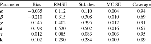
independent replications, which provides evidence of stable estimation and reasonable finite-sample performance. The bias remains small across all parameters, while the RMSE reflects naturally increased variability in tail-related parameters
 $(\gamma, \delta)$
, which is expected in heavy-tailed settings, as summarized in Table 3.
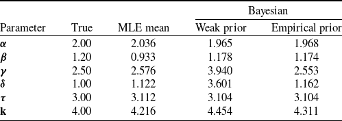
Comparison of true parameters, MLE estimates, and Bayesian posterior means.

Table 2. Long description
A table comparing true parameters, MLE estimates, and Bayesian posterior means. The table has 6 rows and 5 columns. The columns are labeled Parameter, True, MLE mean, Weak prior, and Empirical prior. Row 1: Parameter, True, MLE mean, Weak prior, Empirical prior. Row 2: α, 2.00, 2.036, 1.965, 1.968. Row 3: β, 1.20, 0.933, 1.178, 1.174. Row 4: γ, 2.50, 2.576, 3.940, 2.553. Row 5: δ, 1.00, 1.122, 3.601, 1.162. Row 6: τ, 3.00, 3.112, 3.104, 3.104. Row 7: k, 4.00, 4.216, 4.454, 4.311.
The coverage probabilities are close to the nominal 95% level for most parameters. The small amount of under-coverage for scale parameters
 $(\beta, \delta)$
is observed, which likely reflects the weaker identifiability in the presence of smooth hazard blending. This behavior is consistent with known challenges in composite and extreme-value models and does not affect tail-risk estimation materially. Overall, the results demonstrate stable estimation, accurate uncertainty quantification, and reliable interval performance well across the repeated samples.
Monte Carlo simulation diagnostics (
 $N_{\text{sim}} = 1000$
).

Table 3. Long description
A table comparing Monte Carlo simulation diagnostics for different parameters. The table has six rows and five columns. The columns are labeled Parameter, Bias, RMSE, Std. dev., MC SE, and Coverage. Row 1: Parameter alpha, Bias -0.035, RMSE 0.112, Std. dev. 0.110, MC SE 0.004, Coverage 0.94. Row 2: Parameter beta, Bias -0.210, RMSE 0.315, Std. dev. 0.308, MC SE 0.010, Coverage 0.69. Row 3: Parameter gamma, Bias 0.145, RMSE 0.402, Std. dev. 0.395, MC SE 0.012, Coverage 0.91. Row 4: Parameter delta, Bias 0.198, RMSE 0.520, Std. dev. 0.502, MC SE 0.016, Coverage 0.67. Row 5: Parameter tau, Bias 0.012, RMSE 0.085, Std. dev. 0.083, MC SE 0.003, Coverage 0.95. Row 6: Parameter kappa, Bias 0.102, RMSE 0.290, Std. dev. 0.284, MC SE 0.009, Coverage 0.89.
3.3. Model fit and predictive performance
The MLE and Bayesian inference with weakly informative and empirically centered priors were used to estimate the parameters as shown in Table 2. The MCMC diagnostics indicated excellent convergence, with all
 $\hat{R}$
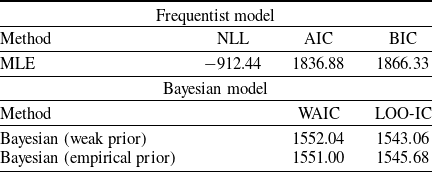
values very close to 1.00 for both weak and empirical priors, and ESSs exceeding 7000+. The well-mixed trace plots for all parameters ensured reliable posterior inference. The fit of the model was assessed using information criteria, mainly AIC and BIC for frequentist MLE, and WAIC and LOO-IC for Bayesian analysis.
The information criteria in Table 4 confirm the superior predictive ability of the Bayesian models, as they outperform the MLE model in terms of model fit. The empirical prior model shows a better performance based on WAIC, while the weak prior model performs better in terms of LOO-IC. The close values indicate that the data dominate in both types of the prior selection.
3.4. Actuarial applications
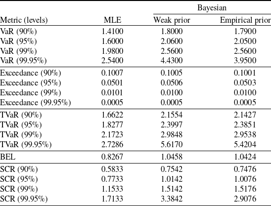
The practical utility of the models was evaluated by computing tail-dependent actuarial risk measures and solvency metrics. Table 5 summarizes the corresponding risk and solvency metrics.
Model fit and predictive performance metrics.

Table 4. Long description
A table comparing model fit and predictive performance metrics. The table has two main sections: Frequentist model and Bayesian model. The Frequentist model section has two rows labeled MLE and columns labeled Method, NLL, AIC, and BIC. The values are: Row 1: Method, MLE; NLL, -912.44; AIC, 1836.88; BIC, 1866.33. The Bayesian model section has two rows labeled Bayesian (weak prior) and Bayesian (empirical prior) and columns labeled Method, WAIC, and LOO-IC. The values are: Row 1: Method, Bayesian (weak prior); WAIC, 1552.04; LOO-IC, 1543.06. Row 2: Method, Bayesian (empirical prior); WAIC, 1551.00; LOO-IC, 1545.68.
Estimated risk measures and solvency measures at different confidence levels.

Table 5. Long description
A table comparing risk and solvency measures at different confidence levels. The table has 11 rows and 4 columns. The columns are labeled MLE, Weak prior, and Empirical prior under the Bayesian header. The row labels include VaR at different percentiles (90 percent, 95 percent, 99 percent, 99.95 percent), Exceedance at different percentiles (90 percent, 95 percent, 99 percent, 99.95 percent), TVaR at different percentiles (90 percent, 95 percent, 99 percent, 99.95 percent), BEL, and SCR at different percentiles (90 percent, 95 percent, 99 percent, 99.95 percent). Row 1: VaR (90 percent), MLE 1.4100, Weak prior 1.8000, Empirical prior 1.7900. Row 2: VaR (95 percent), MLE 1.6000, Weak prior 2.0600, Empirical prior 2.0500. Row 3: VaR (99 percent), MLE 1.9800, Weak prior 2.5600, Empirical prior 2.5600. Row 4: VaR (99.95 percent), MLE 2.5400, Weak prior 4.4300, Empirical prior 3.9500. Row 5: Exceedance (90 percent), MLE 0.1007, Weak prior 0.1005, Empirical prior 0.1001. Row 6: Exceedance (95 percent), MLE 0.0501, Weak prior 0.0506, Empirical prior 0.0503. Row 7: Exceedance (99 percent), MLE 0.0101, Weak prior 0.0100, Empirical prior 0.0100. Row 8: Exceedance (99.95 percent), MLE 0.0005, Weak prior 0.0005, Empirical prior 0.0005. Row 9: TVaR (90 percent), MLE 1.6622, Weak prior 2.1554, Empirical prior 2.1427. Row 10: TVaR (95 percent), MLE 1.8277, Weak prior 2.3997, Empirical prior 2.3851. Row 11: TVaR (99 percent), MLE 2.1723, Weak prior 2.9848, Empirical prior 2.9538. Row 12: TVaR (99.95 percent), MLE 2.7286, Weak prior 5.6170, Empirical prior 5.4204. Row 13: BEL, MLE 0.8267, Weak prior 1.0458, Empirical prior 1.0424. Row 14: SCR (90 percent), MLE 0.5833, Weak prior 0.7542, Empirical prior 0.7476. Row 15: SCR (95 percent), MLE 0.7733, Weak prior 1.0142, Empirical prior 1.0076. Row 16: SCR (99 percent), MLE 1.1533, Weak prior 1.5142, Empirical prior 1.5176. Row 17: SCR (99.95 percent), MLE 1.7133, Weak prior 3.3842, Empirical prior 2.9076.
Risk Metrics (VaR and TVaR): The MLE estimates are comparatively optimistic, particularly at the higher confidence levels, where both the VaR and TVaR are lower than the Bayesian estimates. The Bayesian models, especially under empirical priors, yield more conservative tail-risk estimates, with TVaR (99.95%) reaching 5.6170 and 5.4204 under weak and empirical priors, respectively. The exceedance values in Table 5 correspond to the model-based probabilities and closely match their nominal levels. The comparison with empirical exceedance shows a minor deviations in the extreme tail due to finite-sample variability, while remaining broadly consistent.
Solvency Capital Requirements: The BEL of the Bayesian empirical prior model is 1.0424, very close to the empirical mean (1.0433), compared to the lower MLE estimate (0.8267), indicating a more accurate central liability estimate under the Bayesian approach. SCR estimates follow a similar pattern, with Bayesian values consistently exceeding those of the MLE. At the 99.95% confidence level, the Bayesian SCR (2.9076) is substantially higher than the MLE (1.7133), reflecting a more prudent assessment of capital requirements under tail risk.
Reinsurance Pricing: The expected payout is calculated on the selected XoL reinsurance layers, defined by their attachment point and limit, to assess the model performance in risk transfer applications. This characteristic is a significant benefit in risk transfer negotiations as it delivers a more detailed perspective regarding possible liabilities and needed capital requirements. The notation
 $L \text{ xs } A$
denotes a reinsurance layer of width L in excess of attachment point A.
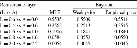
In the smallest layer (0.6 xs 0), all methods produce similar expected payouts, with MLE being marginally higher than the Bayesian estimates, which reflects a slightly strong sensitivity to the fitted distribution. Across intermediate layers (0.4 xs 0.6 and 0.6 xs 1.0), MLE consistently yields higher payouts estimates, while the Bayesian estimates remain slightly lower, which indicates the smoothing effect of parameter uncertainty on the moderate losses. As the attachment point increases further (0.8 xs 1.6 and 2 xs 2.5), all methods produce progressively smaller payouts estimates, which are consistent with diminishing tail probability, with only minor differences across approaches as shown in Table 6.
Expected payouts for reinsurance layers.

Table 6. Long description
A table comparing expected payouts for reinsurance layers using different methods. The table has six rows and four columns. The columns are labeled as Reinsurance layer, MLE, Weak prior, and Empirical prior. The rows are labeled with different reinsurance layers and their corresponding attachment points. Row 1: L equals 0.6 xs A equals 0.0, MLE is 0.5535, Weak prior is 0.5509, Empirical prior is 0.5511. Row 2: L equals 0.4 xs A equals 0.6, MLE is 0.2562, Weak prior is 0.2513, Empirical prior is 0.2515. Row 3: L equals 0.6 xs A equals 1.0, MLE is 0.1906, Weak prior is 0.1841, Empirical prior is 0.1840. Row 4: L equals 0.8 xs A equals 1.6, MLE is 0.0584, Weak prior is 0.0552, Empirical prior is 0.0550. Row 5: L equals 2.0 xs A equals 2.5, MLE is 0.0054, Weak prior is 0.0045, Empirical prior is 0.0045.
This pattern reflects a stable and coherent decline in layer-wise payouts across all models. While MLE produces slightly higher estimates in lower and intermediate layers, the Bayesian approaches yield comparable but smoother estimates. The minimal difference between the Bayes weak and Bayes empirical indicates robustness to the prior specification. These estimates are further supported by the graphical analysis which illustrates the continuous layer payouts and associated uncertainty for reinsurance pricing decisions.
4. Empirical analysis
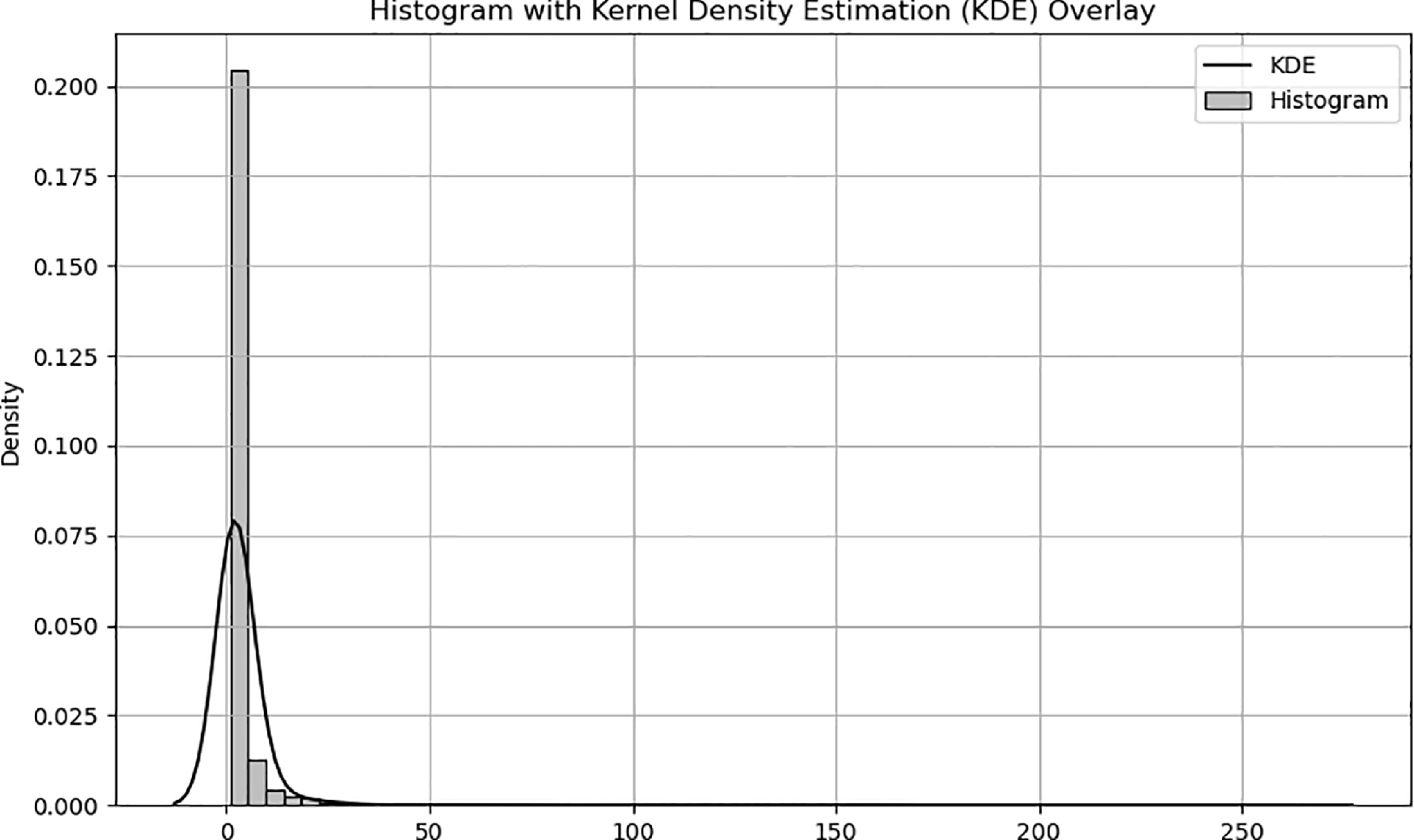
This section presents the empirical validation of the proposed model using the Danish Fire Insurance dataset, which is a well-known benchmark dataset in the extreme value theory and risk management. It comprises of the annual losses (in millions of Danish Kroner) from the major fire events between years 1980 and 1990, as shown in Figure 1. The empirical study focuses on the parameter estimation, risk metrics, and reinsurance analysis.
Histogram of Danish fire insurance losses.

4.1. Descriptive analysis
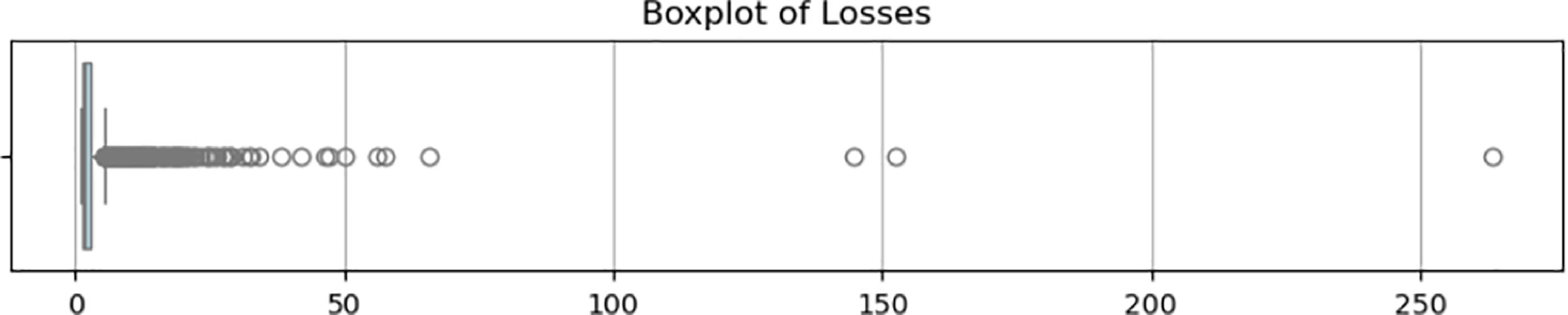
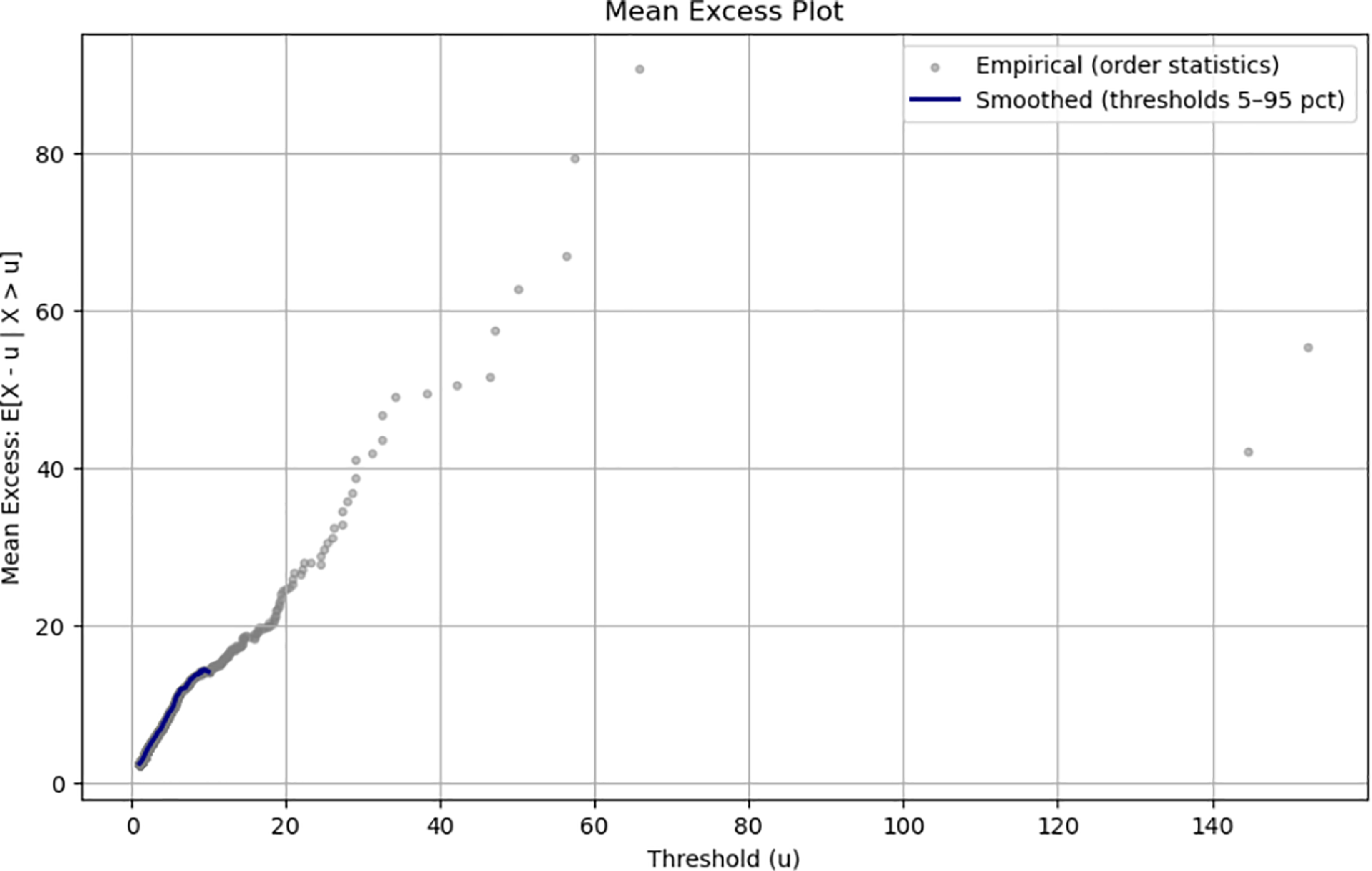
The data exhibit a pronounced heavy-tailed behavior, which reflect the rarity and severity of the extreme losses as confirmed by the boxplot and mean excess plot shown in Figures 2 and 3, respectively.
Box plot of Danish fire insurance losses.

Mean excess plot of Danish fire insurance losses.

Table 7 shows that the median loss is substantially lower than the mean of 3.39 million, which indicate a right-skewed distribution dominated by a few extreme losses. This pronounced skewness and kurtosis confirm a typical leptokurtic pattern in the insurance claim data. The coefficient of variation (2.51) further emphasizes the high relative variability.
4.2. Model estimation and goodness-of-fit
The model parameters are estimated using both the MLE and a Bayesian approach based on the Markov Chain Monte Carlo (MCMC), under the two prior specifications: a weak prior and an empirical prior. The MCMC diagnostics indicated an excellent convergence, with maximum
 $\hat{R}$
values of 1.007 (weak prior) and 1.004 (empirical prior), and ESSs exceeding 39,000, and well-mixed trace plots for all parameters which ensure reliable posterior inference.
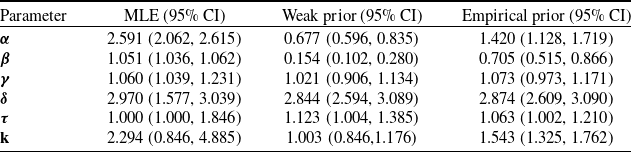
The parameter estimates in Table 8 reveal notable divergence between MLE and the Bayesian posterior means, particularly for the parameters influencing the tail behavior. The transition steepness parameter k, which governs the speed of transition into the tail region, is estimated at 2.294 under MLE and is substantially higher than the Bayesian estimates. This reflects the sensitivity of MLE to the extreme observations and its impact on tail-risk measures (e.g., TVaR at 99.95%) in the finite samples. Confidence intervals for MLE parameters are obtained using the profile likelihood methods, which are robust to the boundary effects and non-quadratic likelihood surfaces. The resulting intervals are not symmetric for several parameters which indicates differing levels of identifiability, particularly for the transition steepness parameter k.
In contrast, the parameters
 $\beta$
,
 $\gamma$
, and
 $\tau$
show strong consistency across all models which indicates robustness in modeling the central structure of the distribution. However,
 $\alpha$
,
 $\theta$
, and k exhibit substantial variation between the two Bayesian priors. The parameter
 $\alpha$
governs the shape of the distribution in the body region and is therefore more sensitive to moderate losses, whereas
 $\beta$
,
 $\gamma$
, and
 $\tau$
primarily control scale and tail behavior. As a result,
 $\alpha$
shows greater variability across estimation methods without materially affecting tail-risk inference. In addition, the empirical prior increases the tail parameter k by 54% relative to the weak prior, reflecting the influence of the prior information on the tail inference and allocation of probability mass. In general, while
 $\beta$
,
 $\gamma$
, and
 $\tau$
are reliably estimated between methods, the variability in
 $\alpha$
,
 $\delta$
, and k drives key differences in the evaluation of tail risk and the performance of the model.
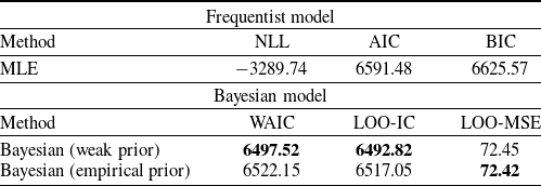
The selection of the best-performing models is based on the AIC, BIC, WAIC, and LOO-IC and LOO-MSE reported in Table 9, which indicate superior predictive performance of Bayesian models relative to MLE. Among them, the weak prior attains the lowest WAIC (6497.52) and LOO-IC (6492.82), suggesting the best out-of-sample predictive accuracy. While both WAIC and LOO-IC assess predictive performance, WAIC is based on posterior predictive density with a variance-based penalty, whereas LOO-IC evaluates accuracy via leave-one-out prediction. In finite samples and heavy-tailed settings, LOO-IC is often more robust, while WAIC provides a computationally efficient alternative. To complement these criteria, LOO-MSE is reported on the original loss scale which provides a direct measure of point-prediction performance. The empirical prior yields a marginally lower LOO-MSE (72.42) compared to the weak prior (72.45) which indicate a slightly improved point prediction, though the difference is negligible.
Descriptive statistics of the loss distribution.

Table 7. Long description
A table with descriptive statistics of the loss distribution. The table has one row and nine columns. The columns are labeled as Min, Quantiles, Max, Mean, Std. dev., CV, Skewness, and Kurtosis. The values in the row are as follows: Min: 1.0000, Quantiles: (1.3211, 1.7782, 2.9670), Max: 263.2504, Mean: 3.3851, Std. dev.: 8.5075, CV: 2.5132, Skewness: 18.7498, Kurtosis: 485.6461.
Parameter estimates under MLE and Bayesian models.

Table 8. Long description
A table with three columns and five rows comparing parameter estimates under MLE, Weak prior, and Empirical prior models. The columns are labeled MLE (95% CI), Weak prior (95% CI), and Empirical prior (95% CI). The rows are labeled with parameters alpha, beta, gamma, delta, tau, and kappa. Each cell contains numerical values representing the estimates and their confidence intervals. Notable trends include varying estimates and confidence intervals across different models, with some parameters showing significant differences between the models.
Model fit and predictive performance metrics.

Table 9. Long description
A table comparing model fit and predictive performance metrics for Frequentist and Bayesian models. The table has two main sections: Frequentist model and Bayesian model. The Frequentist model section has two rows labeled MLE and two columns labeled Method and NLL, AIC, BIC. The Bayesian model section has two rows labeled Bayesian (weak prior) and Bayesian (empirical prior) and three columns labeled Method, WAIC, LOO-IC, and LOO-MSE. Row 1: MLE, -3289.74, 6591.48, 6625.57. Row 2: Bayesian (weak prior), 6497.52, 6492.82, 72.45. Row 3: Bayesian (empirical prior), 6522.15, 6517.05, 72.42.
To further assess the model adequacy beyond the information-criterion-based comparisons, we examine predictive diagnostics using PPCs and calibration measures.
4.3. Model diagnostics and predictive calibration
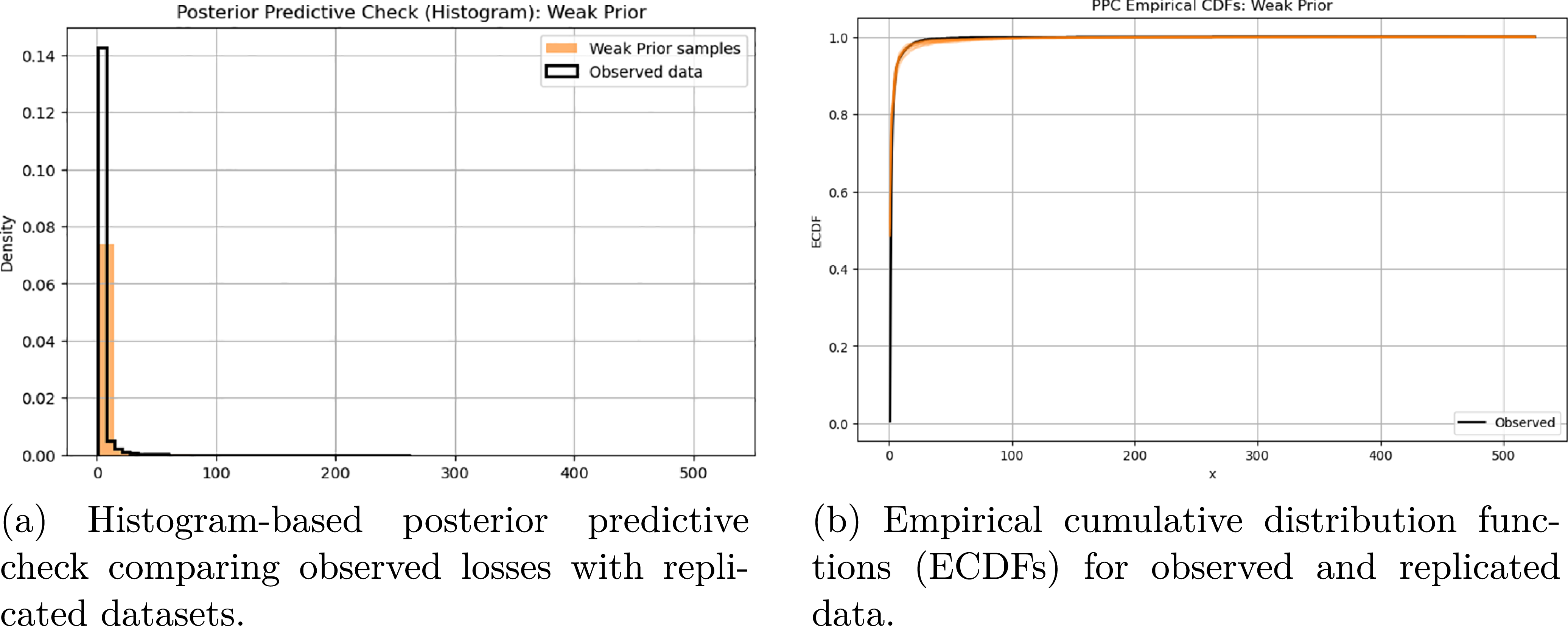
The PPCs shown in Figure 4 show that the Bayesian model reproduces the main features of the observed loss distribution, including the body behavior and the overall tail decay. The discrepancies arise only for the most extreme observations which reflects data sparsity in the tail rather than systematic model mis-specification.
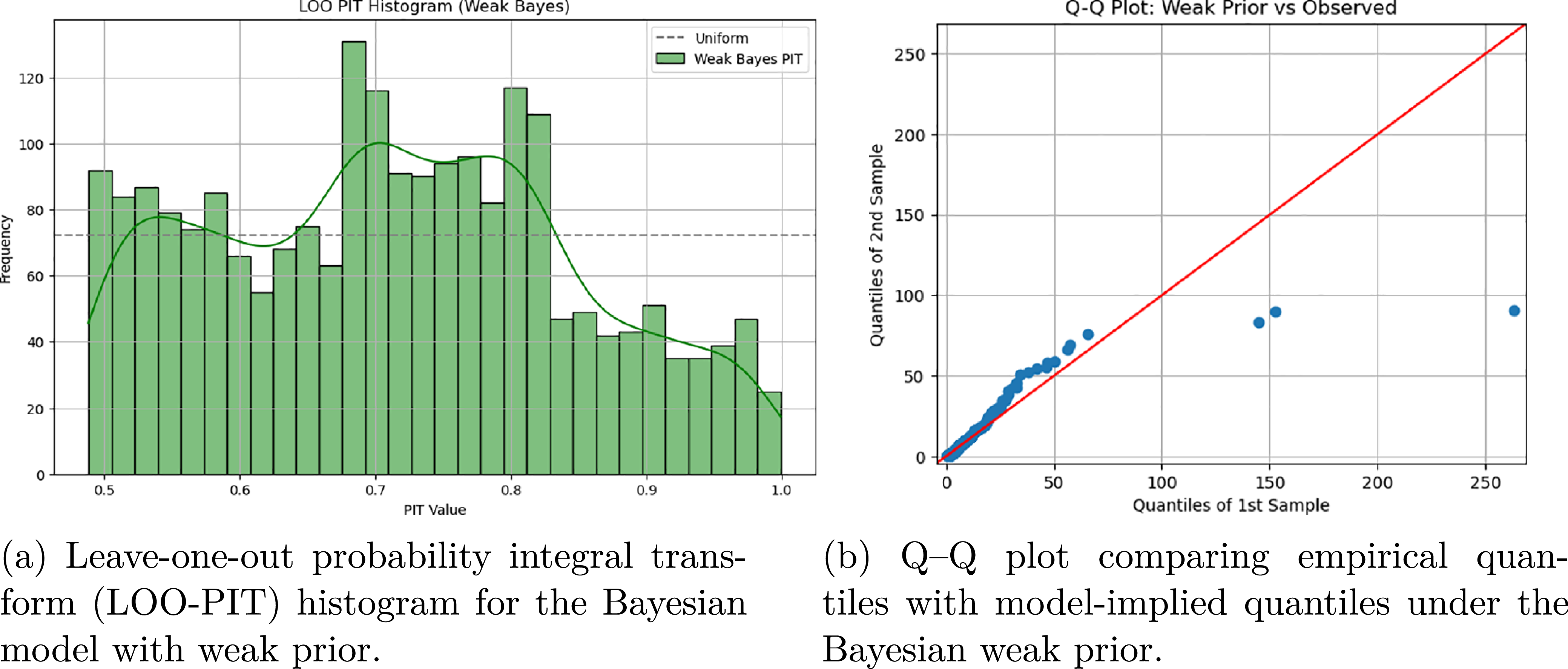
The LOO-PIT diagnostics shown in Figure 5 provide an evidence of adequate predictive calibration for the weak prior model. These mild deviations from uniformity are expected in heavy-tailed severity settings and are consistent with the conservative predictive uncertainty induced by the Bayesian regularization. The accompanying Q–Q plot further supports this conclusion by showing close agreement between the empirical and model-implied quantiles across the body and moderate tail, with deviations confined to the most extreme losses. Together with the PPC results and information criteria, these diagnostics support the weak prior specification as the preferred model.
Posterior predictive checks for the Bayesian model with a weak prior. Panel (a) compares the observed loss distribution with replicated datasets using histogram overlays, while Panel (b) presents the corresponding empirical cumulative distribution functions (ECDFs). The PPCs indicate good agreement in the central region and overall distributional shape, with deviations confined to extreme losses.

Predictive calibration diagnostics for the Bayesian model with weak prior. Panel (a) shows the LOO-PIT histogram, indicating approximate uniformity with mild deviations expected in heavy-tailed settings. Panel (b) presents the Q–Q plot, showing good agreement across the body and moderate tail, with deviations confined to the most extreme losses.

Figure 5. Long description
Panel A: A histogram displays the Leave-one-out probability integral transform (LOO-PIT) for the Bayesian model with a weak prior. The x-axis represents PIT values ranging from 0.5 to 1.0, and the y-axis represents frequency. The histogram bars are green, and a line representing the uniform distribution is overlaid in black. The histogram shows a roughly uniform distribution with some deviations. Panel B: A Q-Q plot compares empirical quantiles with model-implied quantiles under the Bayesian weak prior. The x-axis represents quantiles of the first sample, and the y-axis represents quantiles of the second sample. Data points are plotted in blue, and a red line indicates the ideal agreement line. The plot shows good agreement across the body and moderate tail, with deviations in the most extreme losses.
Classical goodness-of-fit tests such as the Kolmogorov–Smirnov (KS) and Anderson–Darling (AD) statistics are not reported in this study. These tests are typically based on a single fitted CDF and do not account for parameter uncertainty or post-estimation effects which limits their interpretability in composite and Bayesian modeling settings shown by Stephens (Reference Stephens1974) and Choulakian and Stephens (Reference Choulakian and Stephens2001). Moreover, the KS-type tests are known to have a low sensitivity in the tail region, whereas AD-type tests typically require a fully specified closed-form distribution. These assumptions make them less suitable for heavy-tailed loss modeling and extreme risk applications, as explained by Embrechts et al. (Reference Embrechts, Klüppelberg and Mikosch1997). In contrast, Gelman et al. (Reference Gelman, Carlin, Stern, Dunson, Vehtari and Rubin2013) provides PPCs, probability integral transform diagnostics, and leave-one-out predictive criteria which provide a more coherent assessment of distributional fit and predictive performance while explicitly accounting for parameter uncertainty which is particularly important for the tail-risk evaluation.
4.4. Risk and solvency metrics
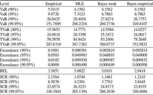
At moderate confidence levels (90%–95%), the empirical and parametric estimates of VaR and TVaR are generally consistent as shown in Table 10. However, at the extreme quantiles (99% and above), the empirical measures are capped by the maximum observed loss and therefore underestimate the tail risk, while MLE and the Bayesian methods extrapolate beyond the data which produces higher values. These differences arise because the empirical estimators suffer from the high variance and a downward bias in the tail, whereas the parametric methods reduce variance at the cost of model dependence. For the solvency regulations purpose, the model-based approaches are preferred for assessing the extreme risk.
Risk and solvency measures at various confidence levels.

Table 10. Long description
The table presents risk and solvency measures at various confidence levels. It has 12 rows and 5 columns. The columns are labeled Level, Empirical, MLE, Bayes weak, and Bayes empirical. The rows are labeled with different confidence levels and measures: VaR (90 percent), VaR (95 percent), VaR (99 percent), VaR (99.95 percent), TVaR (90 percent), TVaR (95 percent), TVaR (99 percent), TVaR (99.95 percent), Exceedance (90 percent), Exceedance (95 percent), Exceedance (99 percent), Exceedance (99.95 percent), BEL, SCR (90 percent), SCR (95 percent), SCR (99 percent), SCR (99.95 percent). Each row contains numerical values corresponding to the measures at different confidence levels. The table provides a detailed comparison of empirical, MLE, Bayes weak, and Bayes empirical methods for assessing risk and solvency.
At the extreme quantiles, the exceedance values remain close to their nominal levels which indicates good internal consistency despite of differences in extrapolated VaR. The empirical BEL (3.3851) exceeds all model-based estimates which indicates that the parametric models slightly understate the central tendency of losses. This downward shift in BEL leads to a higher SCR values, since SCR is defined as the difference between VaR and BEL. The Bayes weak model yields the largest SCR at 99.95% level which reflects greater sensitivity to the parameter uncertainty which closely followed by the MLE-based estimate. In contrast, the lower empirical SCR reflects the absence of extrapolation beyond the largest observed loss which results in underestimation of the extreme capital requirements under finite samples.
The differences between empirical and parametric estimates highlight a practical trade-off in the extreme risk assessment. The empirical methods tend to underestimate tail risk due to the finite-sample limitations, whereas MLE-based approaches are sensitive to the extreme observations which can inflate tail estimates. The Bayesian models offer an intermediate stance, where the weak priors yield more conservative capital estimates, and the empirical priors improve stability and convergence which provides a balance between robustness and conservatism. Although the proposed hazard-blend models achieve strong likelihood-based fit, Table 10 shows that TVaR estimates at the high confidence levels (e.g., 99%) may deviate from empirical counterparts. This behavior is consistent with the known trade-off between likelihood optimization and tail calibration in parametric loss modeling.
Classical extreme-value theory recognizes an inherent bias-variance trade-off in tail calibration. In particular, Coles (Reference Coles2001) and Beirlant et al. (Reference Beirlant, Goegebeur, Segers and Teugels2004) note that tail-focused adjustments may reduce bias in extreme-quantile estimation at the expense of increased estimator variance and sensitivity to modeling choices, while Danielsson et al. (Reference Danielsson, de Haan, Peng and de Vries2001) shows that tuning decisions such as threshold or sample-fraction selection can materially affect the stability of tail estimates in finite samples. From an actuarial perspective, Embrechts et al. (Reference Embrechts, Klüppelberg and Mikosch1997) caution that sensitivity may lead to unstable risk measures when only extreme observations are used for calibration. Accordingly, the present study retains likelihood-based estimation to ensure a coherent comparison between frequentist and Bayesian approaches within a unified framework, while acknowledging that tuning strategies proposed by Mohammad and Cooray (Reference Mohammad and Cooray2025b) can improve tail-focused risk measures when appropriately controlled.
4.5. Reinsurance analysis and expected payouts
The analysis of the expected payout for the different Excess of Loss (XoL) reinsurance layers is undertaken in order to evaluate how the models can price risk at the different attachments. The notation
 $L \text{ xs } A$
denotes a reinsurance layer of width L in excess of attachment point A.
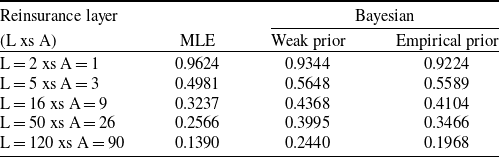
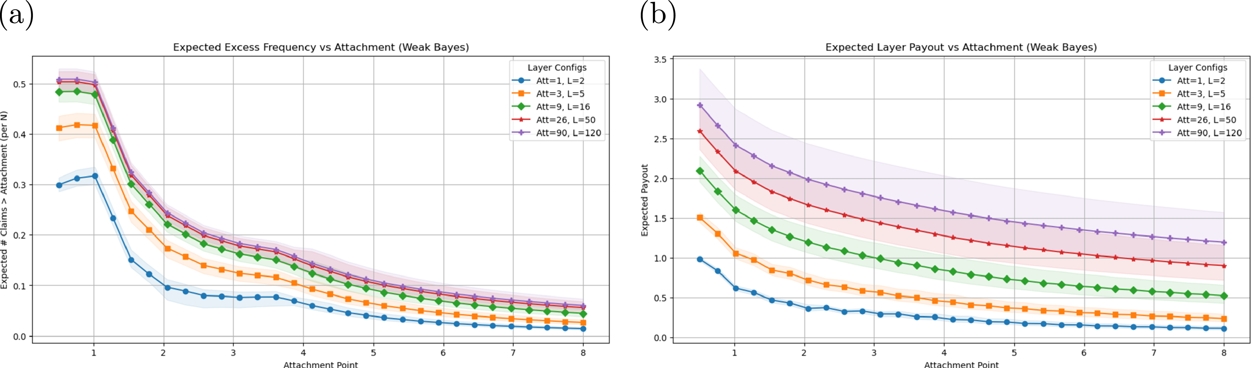
The results in Table 11 indicate that for the lower layers (2 xs 1), all models produce comparable expected payouts and with MLE being marginally higher. As the attachment points and limits increase toward the tail (e.g., 5 xs 3 and 16 xs 9), the Bayesian estimates exceed those of the MLE which reflects greater sensitivity to tail uncertainty. This divergence becomes more pronounced in the extreme layers, where the Bayesian models allocate a higher expected payouts than MLE which is consistent with the heavier tail representation. For the most extreme layer (120 xs 90), the Bayes weak and empirical models yield payouts of 0.2440 and 0.1968, respectively, which are lower as compared to the MLE estimate of 0.1390. Additional diagnostics on the expected layer payouts and the excess claim frequencies for the weak prior model are provided in Appendix B1.
Expected payouts for Excess of Loss (XoL) reinsurance layers.

Table 11. Long description
A table comparing expected payouts for different reinsurance layers using MLE, Bayesian weak prior, and Bayesian empirical prior models. The table has five rows and four columns. The columns are labeled as Reinsurance layer, MLE, Weak prior, and Empirical prior. The rows are labeled with different reinsurance layers: L equals 2 xs A equals 1, L equals 5 xs A equals 3, L equals 16 xs A equals 9, L equals 50 xs A equals 26, and L equals 120 xs A equals 90. The values in the table are as follows: Row 1: L equals 2 xs A equals 1, MLE 0.9624, Weak prior 0.9344, Empirical prior 0.9224. Row 2: L equals 5 xs A equals 3, MLE 0.4981, Weak prior 0.5648, Empirical prior 0.5589. Row 3: L equals 16 xs A equals 9, MLE 0.3237, Weak prior 0.4368, Empirical prior 0.4104. Row 4: L equals 50 xs A equals 26, MLE 0.2566, Weak prior 0.3995, Empirical prior 0.3466. Row 5: L equals 120 xs A equals 90, MLE 0.1390, Weak prior 0.2440, Empirical prior 0.1968.
While from the practical perspective, these differences have an important implications for reinsurance pricing and capital assessment. The MLE provides slightly higher estimates in the lowest layer, as it tends to produce lower expected payouts in the higher layers, while the Bayesian models yield the higher estimates due to improved capture of the tail risk and parameter uncertainty. This highlights a trade-off between sensitivity to observed data and robustness under sparse tail information, with Bayesian methods provides a more reliable framework for the pricing and solvency assessment across reinsurance layers.
5. Conclusion and discussion
The paper presented a smooth hazard-blend composite distribution that combines a Weibull body with a Pareto tail which are estimated under both the frequentist and Bayesian frameworks. By operating directly on the hazard scale, the proposed construction ensures that the global continuity and differentiability of the cumulative hazard and survival functions which overcome the key limitations of the traditional spliced composite models at the transition points.
The simulation results show that the proposed model is capable of flexibly representing both the central and extreme regions of the loss distribution. In particular, the Bayesian inference displays an improved numerical stability and the predictive calibration relative to MLE, particularly in the heavy-tailed settings. The comparison between weakly informative and empirical priors highlights the sensitivity of tail-risk measures to the prior specification and, therefore, the need for a transparent and context-aware prior choices in the actuarial applications.
The empirical analysis using the Danish fire insurance dataset confirms the practical relevance of the framework. For moderate confidence levels (90%–95%), the empirical and parametric risk measures are closely aligned, while at the higher confidence levels (99%–99.95%) the parametric extrapolation becomes essential. The empirical estimators tend to underestimate extreme risk due to the finite-sample limitations, whereas the Bayesian hazard-blend models provide a more coherent tail extrapolation while accounting for the parameter uncertainty. In particular, the weak-prior Bayesian specification provides conservative but stable estimates of the extreme risk which is consistent with regulatory solvency objectives.
In the context of the XoL reinsurance, the Bayesian hazard-blend models produce a more stable and credible expected layer payouts, especially for the higher attachment points where tail uncertainty dominates. While MLE estimates are sensitive to extreme observations which can lead to unstable layer pricing, the Bayesian methods regularize tail behavior through posterior uncertainty, supporting more robust pricing and capital assessment. Thus, the proposed hazard-blend framework provides a principled and practically feasible approach for the loss modeling, reinsurance pricing, and solvency assessment in modern actuarial practice.
6. Future research
The proposed hazard-blend framework admits several natural extensions that could enhance both the theoretical scope and practical applicability. First, alternative body–tail combinations may be extended to more flexible or heavy-tailed specifications, such as Burr bodies coupled with lognormal, generalized Pareto or tempered stable tails, allowing closer alignment with severity profiles across different portfolios and geographic regions. Second, the current static univariate formulation may be extended to more dynamic or semi-parametric settings by incorporating covariates through regression structures or generalized additive models (GAMs) which enables the time-varying scale and tail behavior for forward-looking pricing and risk assessment.
Third, the tuning-based parameter adjustment methods, such as those proposed by Mohammad and Cooray (Reference Mohammad and Cooray2025b), could be integrated within the hazard-blend framework to improve the calibration of the extreme tail-risk measures (e.g., TVaR) by balancing likelihood fit and tail accuracy. An important direction for future research is the development of principled tuning strategies that also control estimator variance which provide a more systematic mechanism for tailoring the model to regulatory or risk management settings where conservative tail behavior is prioritized.
Additional extensions include stress testing under regulatory regimes such as Solvency II, ICS, NAIC RBC, as well as multivariate generalizations using copulas or hierarchical Bayesian structures, and computational approaches such as variational inference or INLA for scalable estimation. The development of user-friendly implementations in R or Python, with built-in diagnostics and risk metrics, would further support practical adoption.
Acknowledgments
The authors would like to thank the reviewers and the editor for their constructive comments and valuable suggestions, which helped improve the quality of this manuscript. The authors acknowledge the Department of Science and Technology (DST), Government of India, for infrastructural support through the DST-FIST (Fund for Improvement of S&T Infrastructure) program at the Department of Mathematics and Statistics, Central University of Punjab, Bathinda. The authors are thankful to the Central University of Punjab for providing research support and a conducive academic environment.
Competing interests
The authors declare no conflict of interest.
Data availability statement
The Danish Fire Insurance dataset analyzed in this study is publicly accessible through the CASdatasets package in R and on the authors’ public GitHub repository at https://github.com/mohitlamba49/Composite-Hazard-Blend. All analyses were performed in Python using standard statistical and Bayesian inference libraries. Algorithmic descriptions and selected executable components supporting the analysis are also provided in the same public GitHub repository.
Appendices
A. Robustness analysis of composite model specification
To assess the robustness of the proposed composite modeling framework, we conduct two sensitivity analyses: (i) alternative blending weight functions and (ii) alternative body–tail distribution combinations. All models are estimated using maximum likelihood and evaluated using both in-sample and predictive criteria.
A.1 Alternative blending weight functions
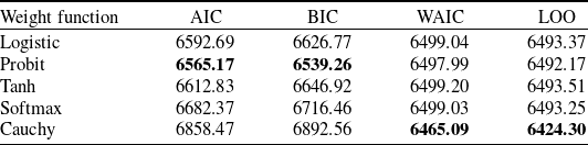
The proposed model employs a smooth transition between body and tail components through a blending weight function. To examine sensitivity, we consider logistic, probit, tanh, Cauchy, and softmax specifications.
Model comparison across alternative blending weight functions.

Table A1. Long description
A table comparing model performance across different weight functions using AIC, BIC, WAIC, and LOO metrics. The table has five rows and five columns. The columns are labeled Weight function, AIC, BIC, WAIC, and LOO. The rows are labeled Logistic, Probit, Tanh, Softmax, and Cauchy. Row 1: Logistic, AIC 6592.69, BIC 6626.77, WAIC 6499.04, LOO 6493.37. Row 2: Probit, AIC 6565.17, BIC 6539.26, WAIC 6497.99, LOO 6492.17. Row 3: Tanh, AIC 6612.83, BIC 6646.92, WAIC 6499.20, LOO 6493.51. Row 4: Softmax, AIC 6682.37, BIC 6716.46, WAIC 6499.03, LOO 6493.25. Row 5: Cauchy, AIC 6858.47, BIC 6892.56, WAIC 6465.09, LOO 6424.30.
Logistic, tanh, and softmax functions exhibit nearly identical performance, reflecting similar smooth transition behavior. Although probit attains slightly lower AIC, differences in WAIC and LOO among these specifications are negligible in practical terms, as noted by Hosmer et al. (Reference Hosmer, Lemeshow and Sturdivant2013), Agresti (Reference Agresti2013). The Cauchy-based weight achieves the lowest WAIC and LOO, indicating greater sensitivity to extreme observations, but its higher AIC and BIC suggest potential overfitting.
The logistic specification is retained for its simplicity, interpretability, and numerical stability, as emphasized by Teräsvirta (Reference Teräsvirta1994) and Bishop (Reference Bishop2006). It is preferred over the probit specification due to its fully closed-form expression and computational convenience as emphasized by Bishop (Reference Bishop2006), Hastie et al. (Reference Hastie, Tibshirani and Friedman2009), and Gelman et al. (Reference Gelman, Carlin, Stern, Dunson, Vehtari and Rubin2013), and it is standard in smooth transition modeling frameworks, as further discussed by Teräsvirta et al. (Reference Teräsvirta, Tjøstheim and Granger2010). The Cauchy weight is discarded due to its overemphasis on extreme observations, which makes it more prone to overfitting and less stable in practice.
A.2 Alternative composite distribution specifications
We further assess robustness by considering alternative body–tail combinations within the same hazard-based framework, while retaining the Pareto distribution for the tail while varying the body distribution.
Model comparison across alternative composite distributions.

Table A2. Long description
A table comparing different composite models using various statistical metrics. The table has four rows and five columns. The columns are labeled Composite model, AIC, BIC, WAIC, and LOO. The rows are labeled Weibull–Pareto, Lognormal–Pareto, and Gamma–Pareto. Row 1: Weibull–Pareto, AIC, 6562.39, BIC, 6596.47, WAIC, 6337.18, LOO, 6287.49. Row 2: Lognormal–Pareto, AIC, 6548.99, BIC, 6583.07, WAIC, 6381.90, LOO, 6318.53. Row 3: Gamma–Pareto, AIC, 6570.68, BIC, 6604.77, WAIC, 6471.36, LOO, 6419.94.
The lognormal–Pareto model achieves the lowest AIC and BIC, indicating better in-sample fit, but performs worse in WAIC and LOO than the Weibull–Pareto model, suggesting weaker predictive stability. The Weibull–Pareto model consistently achieves the lowest WAIC and LOO, indicating superior predictive performance, while the gamma–Pareto model underperforms across all criteria.
Overall, the results show robustness of the proposed framework to both blending functions and distributional assumptions. While some alternatives improve in-sample fit, the Weibull–Pareto model with a logistic transition offers a stable, interpretable, and competitively performing specification, supporting its use in the main analysis.
B. Additional actuarial diagnostics
Additional actuarial diagnostics are reported in Figure B1 to illustrate the behavior of the weak prior specification across a range of reinsurance structures. In particular, the expected reinsurance layer payouts and excess claim frequencies are evaluated as functions of the attachment point. These results complement the main analysis by demonstrating the stability and consistency of the proposed model under varying reinsurance configurations.
Weak prior reinsurance diagnostics. (a) Expected layer payout as a function of the attachment point. (b) Expected excess claim frequency above the attachment point. Shaded regions indicate 95% posterior credible intervals.

C. Benchmark composite models
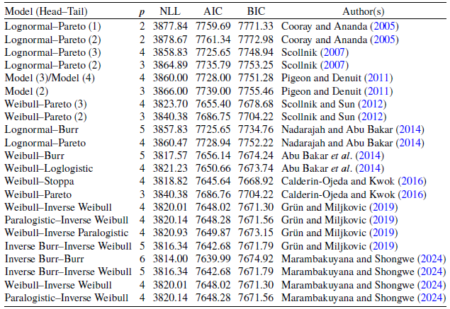
Table C1 summarizes the results previously reported for the Lognormal–Pareto and Lognormal–Burr composite models, together with several composite models featuring Weibull and other distributions in the body and various parametric distributions in the tail. These models and their corresponding statistics are documented in Cooray and Ananda (Reference Cooray and Ananda2005), Scollnik (Reference Scollnik2007), Pigeon and Denuit (Reference Pigeon and Denuit2011), Scollnik and Sun (Reference Scollnik and Sun2012), Nadarajah and Abu Bakar (Reference Nadarajah and Abu Bakar2014), Abu Bakar et al. (Reference Abu Bakar, Hamzah, Maghsoudi and Nadarajah2014), and Calderin-Ojeda and Kwok (Reference Calderin-Ojeda and Kwok2016). Furthermore, recent models from Grün and Miljkovic (Reference Grün and Miljkovic2019) and Marambakuyana and Shongwe (Reference Marambakuyana and Shongwe2024) are incorporated, which reflect the ongoing advances in the composite loss modeling for the Danish Fire Insurance dataset.
Comparison of composite models: parameters, NLL, AIC, and BIC of Danish fire insurance dataset.

Table C1. Long description
The table compares various composite models used for the Danish fire insurance dataset. It includes columns for Model (Head-Tail), p, NLL, AIC, BIC, and Author(s). The table has 21 rows and 6 columns. Each row represents a different model with corresponding values for p, NLL, AIC, and BIC, along with the authors who documented the model. Notable models include Lognormal-Pareto, Lognormal-Burr, Weibull-Pareto, and others. The table captures the ongoing advances in composite loss modeling for the dataset.


 Nsim=1000