

1 Introduction
Those who advise individual investors, design pension plans, and assess public policy proposals often assume that individuals need to save enough to replace 75–80% of their pre-retirement income during retirement. For example, Scheiber (Reference Scheiber2007) states:
By the end of the 20th century, most pension analysts estimated that retirement income needed to be around 75 to 80 percent of final pay for workers to maintain their achieved standard of living during retirement. (Scheiber, 2007. p. 22).
This rule of thumb traces back to the Interim Report of the President's Commission on Pension Policy published in 1980. A ratio of less than 100% accounts for the fact that income saved prior to retirement need not be replaced and the fact that effective tax rates typically decline upon retirement. Building off of the 1980 President's Commission report, Aon Consulting/Georgia State University (2004) (hereafter, Aon/GSU) has been reporting target replacement rates since 1988. Some more recent studies have concluded that the consensus replacement rate target is too low. For example, Alford, Farnen, and Schachet (Reference Alford, Bryan Farnen and Schachet2004) suggest adequate replacement rates range from 75 to 90% of pre-retirement income; and Steinberg and Lucas (Reference Steinberg and Lucas2004) suggest adequate replacement rates range from 85 to 95%. Target replacement rates have been used not only by investment advisors and pension plan consultants, but also by analysts to evaluate public policy. For example, Munnell, Webb, and Delorme (Reference Munnell, Webb and Delorme2006) use a replacement rate method to produce a ‘National Retirement Risk Index’. The US Government Accountability Office (GAO) (2007) uses replacement rates to assess the effectiveness of the private pension system. Scheiber (Reference Scheiber2007) uses replacement rates to estimate the cost of providing pension benefits.
This paper reexamines the issue of what constitutes retirement adequacy. Calculations of retirement savings adequacy based on traditional replacement rate methods suffer from at least three shortcomings: the replacement rates are calculated using nominal retirement income, typically with nominal final pay as the denominator; the analysis fails to treat savings as endogenous; and the analysis does not properly account for owner-occupied housing. The simulations in this study show that savings and investment behavior judged by standard analysis to be inadequate actually results in high real consumption in retirement relative to pre-retirement consumption. For example, the assumed savings and investment behavior of single individuals in the simulations results in traditional replacement rate measures – that is, gross retirement income to gross final pay – of approximately 60%, well below the adequacy threshold of 75–80%. However, these ratios correspond to consumption replacement rates of about 90% for renters and over 100% for homeowners who have paid off their mortgage.
Typical replacement rate measures compare income during the first year of retirement to income during the year (or years) prior to retirement. However, the intuition provided by standard life-cycle models is that individuals generally wish to smooth consumption over their lifetime.Footnote 1 As noted by Sabelhaus (Reference Sabelhaus1997), replacement rate measures should reflect the goal of replacing pre-retirement consumption, rather than replacing earnings, income, or even expenditures, in any given year. In addition, replacement rates are typically calculated using nominal measures of retirement resources. To the extent that retirement income is fixed in nominal terms, income in the first year of retirement will overestimate average real consumption in retirement.Footnote 2
Even if a target replacement rate were to be measured properly, it is typically used improperly when determining what represents an adequate level of retirement savings. As noted above, some level of pre-retirement savings is assumed when determining how much income needs to be replaced during retirement. However, once the target replacement rate is estimated, the target is often used, in turn, to calculate the amount of savings needed to attain the goal. Calculations in this second stage typically fail to treat savings as endogenous.Footnote 3 That is, despite the fact that the target replacement rate is a function of the savings rate, the savings rate needed to achieve ‘adequate’ retirement resources is typically not consistent with the savings rate assumed to calculate ‘adequate’ retirement resources. For example, Aon/GSU (2004) assumes savings rate between 2.2 and 4.0% of income prior to retirement, depending upon the individual's level of income, when calculating target replacement rates (Aon/GSU 2004, p. 11). The study then concludes that to achieve the target replacement rate, individuals who begin to save at age 25 would need to save more in all cases (between 3.1 and 6.8% of pay, depending on their income) than was assumed in calculating the target rates.Footnote 4
Finally, replacement rate studies typically do not properly account for home equity, which represents a large portion of wealth for many households. The proper treatment of owner-occupied housing has been debated in the literature. Venti and Wise (Reference Venti and Wise1991) argue that because retirees typically do not liquidate their housing wealth – by selling their house, downsizing, or taking out a reverse mortgage – housing wealth should not be considered when determining retirement savings' adequacy. Mitchell and Moore (Reference Mitchell and Moore1998) include housing wealth in replacement rate measures. Munnell, Webb, and Delorme (Reference Munnell, Webb and Delorme2006) annuitize all housing wealth, but adds a measure of imputed rent to pre-retirement income. The question of weather or not home equity should be considered when calculating retirement savings' adequacy has in turn spurred a literature that examines housing wealth during retirement.Footnote 5
To a large extent, whether or not retirees liquidate their housing wealth is not of first-order importance with regard to calculating target replacement rates. The primary benefit of owner-occupied housing is that it supplies rental services in excess of expenses. That is, if a household did not own a home, they would be required to pay rent to live in one. Whether the asset is liquidated or not, households with their own home are better-off than otherwise identical households that live in rented houses; that is, homeowners need less cash income during retirement. It is possible that retirees could improve their well-being by liquidating some or all their housing wealth.Footnote 6 However, empirical evidence that retirees liquidate housing wealth is not required to conclude that equity in owner-occupied housing increases retirement resources.
In addition to addressing the shortcomings of typical replacement rate measures, this paper is also intended to be heuristic: representative examples are designed to illustrate the factors that influence measures of retirement adequacy. The paper is organized as follows. Section 2 discusses the assumptions used in the simulations. Section 3 presents the baseline results. Section 4 shows how the results change when savings, taxes, and owner-occupied housing are incorporated into the measure. Section 5 simulates how replacement rate measures would change under alternate Social Security reform proposals. Section 6 illustrates the sensitivity of the results to changes in the underlying assumptions. Conclusions of the paper have been drawn in Section 7.
2 Assumptions used in the simulations
Replacement rate measures are illustrated by creating representative households and simulating their savings and spending behavior over a lifetime. The representative individuals in the simulations are assumed to be born on January 1, 1966. These individuals are of age 40 in 2006, and would reach their normal retirement age of 67 in 2033. Earnings paths are constructed that roughly represent median earnings for workers with various levels of education. For a given earnings path, individuals or married couples follow an assumed savings path. Married couples are assumed to be the same age. Retirement income is assumed to be derived from two sources: Social Security benefits and payments derived from accumulated savings.
2.1 Earnings paths
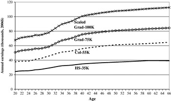
The representative earnings paths are anchored at the approximate median earnings of workers for workers aged 40 with a high school degree ($35,000 in 2006 dollars), a bachelor's degree ($55,000), and a graduate degree ($75,000). In addition, a fourth earnings path one-third higher than the median graduate degree (i.e., $100,000) is calculated. The series are plotted in Figure 1.Footnote 7 The names of the series reflect their origin: (1) HS-35K (high school graduate earning $35,000 in 2006 dollars); (2) Col-55K (college graduate earning $55,000 in 2006 dollars); (3) Grad-75K (worker with a graduate degree earning $75,000 in 2006 dollars); and (4) Scaled Grad-100K.
Representative earnings paths

Conclusions regarding resource adequacy are made in reference to the earnings paths, not to levels of education. For each earnings path, I will look at replacement rates for single individuals, for married couples with one earner, and for married couples with each individual earning being half of total household earnings. The examples are meant to be flexible in that they provide a range of simulated results for a given earnings path. This should allow the reader to approximate what results would be for, say, a married couple with similar total earnings but with a different composition of earnings.
2.2 Social Security, savings, and income during retirement
Income during retirement is assumed to come from only two sources: Social Security benefits and income generated by financial assets accumulated in a worker's 401(k) account. Economic and demographic assumptions used in the simulations are consistent with those used by the Social Security Administration (SSA) in their intermediate projection (SSA, 2006).
2.2.1 Social Security benefits
Workers are assumed to work until normal retirement age, which, in the case of these examples would be 67 years in the year 2033. Parameters for the calculation of Social Security benefits use either historic values (for 2006 and years prior to 2006) or are consistent with the SSA's 2006 intermediate projection. Most parameters used in the calculation are indexed to wage growth, using the average wage index (AWI). The SSA's intermediate projection has average real wages growing by a steady 1.1% a year after 2015, with nominal wage growth of 3.9% and inflation of 2.8%. The initial benefit is indexed to inflation in the years after retirement.Footnote 8
For each earnings path, I calculate three Social Security benefit levels: assuming the earnings are for a single individual; for a single-earner married couple; and for a married couple with each spouse earning one-half of total earnings (hereafter, ‘dual-earner married couple’). For any given earnings path, married couples receive more through Social Security benefits than single individuals. In the case of single-earner married couples, this is because the non-working spouse is eligible for Social Security benefits equal to 50% of the working spouse's benefit. In the case of dual-earner married couples, this is because of the progressivity of the benefits formula: because each spouse earns half the amount of the single individual, their benefits replace a higher proportion of earnings.
2.2.2 Savings and income from financial Assets
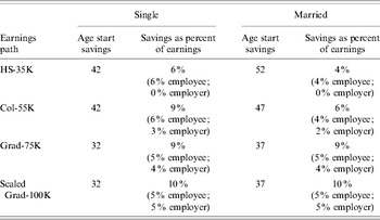
Table 1 summarizes the assumptions regarding the savings behavior used in the simulations. These assumptions are simply meant to be behavior that a priori seemed reasonable to the author. Generally, no post-simulation adjustments were made to calibrate the assumptionsFootnote 9 and they were not chosen to represent ‘optimal’ savings paths. All savings are assumed to accumulate within, and receive the tax treatment of, a 401(k) plan. Contributions to 401(k) plans as a percent of earnings, inclusive of any employer match, range from 4% a year for married couples with the HS-35K earnings path to 10% a year for those with the Scaled Grad-100K earnings path. The age at which workers start contributing to a 401(k) plan ranges from age 32 for single individuals with the Scaled Grad-100K earnings path to age 52 for married couples with the HS-35K earnings path. Those with higher earnings paths contribute a higher percentage of earnings and start contributing at an earlier age. Similarly, because they have more earnings on a per-person basis, single individuals are assumed to begin contributing at an earlier age than married couples with the same earnings path and, in the case of HS-35K and Col-55K, earners contribute a higher percentage of earnings. It is also assumed that higher earners work for employers with more generous matching formulae.
Savings behavior assumptions by earnings path and marital status

Source: Author's assumptions.
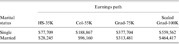
Contributions to a 401(k) are assumed to be invested in inflation-indexed Treasury bonds, also known as Treasury inflation-protected securities (TIPS). Yields are assumed to be 2.4% real, which, through most of the projection period, yields a nominal rate of 5.2%.Footnote 10Table 2 reports the amount of assets accumulated by the time a worker retires by earnings and marital status. Those with higher earnings are assumed to accumulate more in assets because they have higher earnings, contribute a higher proportion of their earnings, and begin contributing at an earlier age. Controlling for total earnings, single individuals accumulate more because they are assumed to begin saving at an earlier age. For married couples, assets at retirement (in 2006 dollars) range from $28,245 for HS-35K earners to $464,417 for Scaled Grad-100K earners. For single individuals, assets range from $77,709 to $559,562.
Simulated asset accumulation at retirement (2006$)Footnote 1
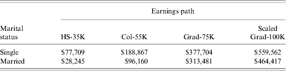
Source: Author's calculations.
1 Assumes savings are invested in inflation-indexed bond earning 2.4% real; inflation rates taken from history and Social Security Administration's Intermediate Projection.
Upon retirement, it is assumed that the entire 401(k) balance is used for purchasing an immediate real life annuity. That is, an annuity is purchased that provides an annual payment until death and adjusts the payment each year to account for changes in the cost of living. Pricing for the annuity was obtained from the Vanguard website.Footnote 11 Because the SSA's intermediate projection assumes life expectancy at age 65 will increase 1.9 years for males and 1.5 years for females between 2005 and 2035, annuity prices in 2033 for a 67-year-old individual or couple are assumed to be equal to annuity prices in 2006 for a 65-year-old individual or couple. Because females have longer life expectancies than males, an annuity for a female provides less income for any given amount invested.
2.3 A baseline replacement rate measure
Replacement rates typically compare retirement income to pre-retirement income. To calculate retirement income in the first year of retirement, most replacement rate studies convert accumulated assets to an income stream by assuming the assets are used for purchasing a fixed nominal annuity. This is then compared to income in the year (or years) prior to retirement. For example, Aon/GSU (2004) and Steinberg and Lucas (Reference Steinberg and Lucas2004) use income in the year prior to retirement. Holden and Van Derhei (Reference Holden and VanDerhei2005) and Purcell and Whitman (Reference Purcell and Whitman2007) compare income generated in the first year of retirement to the average income received in the five years prior to retirement. Although not typical, others use some measure of average earnings. For example, SSA (2006), Munnell, Webb, and Delorme (Reference Munnell, Webb and Delorme2006), and GAO (2007) use average lifetime earnings, with the earnings indexed to wage growth.
As a first step to improving measures of retirement resource adequacy, this section makes two changes to the typical replacement rate measure. First, as noted above, it is assumed a real – rather than nominal – immediate life annuity is purchased at retirement. A real annuity is more consistent with the goal of smoothening real consumption during retirement. Second, the replacement rate measures average real income in retirement relative to average real earnings prior to retirement. Using measures of average real earnings and average real retirement income is a step toward measuring a consumption replacement rate. Average earnings are more likely to be correlated with average pre-retirement consumption than earnings in any given year. Average retirement income is more likely to be correlated with average retirement consumption than is income in the first year of retirement, particularly if any portion of income is fixed in nominal terms. Using average earnings indexed to inflation rather than to wage growth more accurately measures potential real lifetime consumption.Footnote 12
Both the numerator and denominator of the replacement rate differ slightly from simple averages. Given the sharp increase in earnings in the early part of working careers, especially for those with higher education, and acknowledging that some tastes – such as the willingness to share living quarters with unrelated individuals – may change over time, only earnings after age 30 are included in the real earnings average. The formula for the numerator is:

where B=real Social Security benefit; S=real income from accumulated savings; Pr(alive)t=probability individual (or both spouses of a married couple) alive at age 67 is alive at age t;Footnote 13 and t indexes the age of the individual.Footnote 14
This measure is weighted by survival probabilities, and thus places greater weight on income received in the early years of retirement.
Given that both Social Security benefits and annuity income are indexed to inflation in the simulations, the measure of average retirement income may seem overly complex. However, the measure is used because later simulations will incorporate Federal and state income taxes, which are not fully indexed to inflation. In addition, this study is primarily about measurement methods, and this measure can be used in analyzing alternative payout schemes, such as nominal annuities or periodic payments from a pool of investments.
3 Results from the baseline simulation
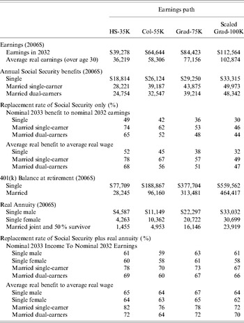
Results from the baseline simulation are presented in Table 3. All reported dollar amounts are in 2006 dollars. The individuals or married couples simulated are assumed to retire at the age of 67 in the year 2033. The top panel shows the earnings of the individual or couple in 2032, the year prior to retirement, as well as the average earnings after age 30. Because real earnings increase over time in the earnings paths used, average real earnings for each series are higher than real earnings at age 40, and the earnings in the year prior to retirement are higher than average earnings. For example, for the Col-55K earnings path, average real earnings after age 30 are $58,306 and earnings in 2032 are $64,644.
Results from baseline case simulationFootnote 1

Source: Author's calculations.
1 Assumes savings are invested in inflation-indexed bond earning 2.4% real; inflation rates taken from history and Social Security Administration's Intermediate Projection. At retirement, real annuity purchased, with pricing for annuity taken from Vanguard's annuity website on October 31, 2006.
For each earnings series, the next lower panel shows the annual Social Security benefit that individuals and married couples would receive. For single individuals, the annual benefits range from $18,814 for the HS-35K earnings path to $33,315 for the Scaled Grad-100K earnings path. As noted above, controlling for total earnings, married couples receive higher benefits. For example, for the Col-55K earnings path, single-earner married couples would receive $39,187 annually and dual-earner married couples would receive $32,547 annually, compared to $26,124 for single individuals.
The next panel shows, for Social Security benefits only, a typical replacement rate measure that compares nominal benefits in the year 2033, the first year of retirement, to nominal earnings in 2032, the final year of earnings. Social Security replacement rates are higher for lower earners and for married couples. For single individuals, replacement rates range from 49% for the HS-35K earnings path to 30% for the Grad-100K earnings path. Replacement rates for married single-earners range from 74 to 46%, and range from 65 to 44% for married dual-earners. Presented below the nominal replacement rate is the preferred measure of replacement: real average income in retirement compared to real average earnings.Footnote 15 Given that Social Security benefits are indexed for inflation and that average real earnings are not much below real earnings at age 66, the preferred measure is not radically different from standard replacement rates, typically higher by 3 or 4 percentage points.Footnote 16
Income derived from 401(k) plans is reported in the bottom half of the table. In the simulations, single individuals accumulate between $77,709 (for the HS-35K earnings path) to $559,562 (for the Scaled-Grad 100K earnings path). With these balances, single males could purchase real annuities providing annual income ranging from $4,587 for those with the HS-35K earnings path to $33,032 for those with the Scaled Grad-100K earnings path. Because females typically live longer than males, annual annuity payments for single females are 7% lower.
Because they start saving later in life, and in the case of the HS-35K and Col-55K earnings path save less, married couples accumulate fewer assets, controlling for total earnings. Married couple 401(k) balances range from $28,245 to $464,417. Married workers were assumed to purchase joint and 50% survivor annuities. That is to say, upon the death of a spouse, the surviving spouse would continue to receive one-half of the original annuity payment. With less money to invest – both absolutely and on a per-person basis – married couples can purchase annuities with annual payments ranging from $1,455 for HS-35K workers to $23,919 for Scaled Grad-100K workers.Footnote 17
Replacement rates for retirees that take into account both Social Security benefits and annuity income are presented in the lowermost panel of Table 3. Using a typical measure, replacement rates for single individuals are near 60% for all of the earnings paths, with males having a slightly higher replacement rate than females because of higher annuity payments. Married one-earner couples have replacement rates ranging from 78% for HS-35K workers to 67% for Scaled Grad-100K workers. Because of lower Social Security benefits, married dual-earner couples have lower replacement rates, holding total earnings fixed, and this is most pronounced at lower earnings levels. Once again, the preferred replacement rate, which compares average real income during retirement to average real earnings, produces replacement rates that range from 3 to 6 percentage points higher than the standard measure. Through the remainder of the paper, only replacement rates that compare average real income during retirement to average real earnings are presented.
4 Adjusting for savings, taxes, and owner-occupied housing
As noted above, the goal of this exercise is to create a replacement rate measure that corresponds as closely as possible to the replacement rate of consumption. One adjustment to typical replacement rates has already been made: using average measures of earnings and retirement income expressed in real dollars. However, neither gross income nor gross earnings measure potential consumption. First, earnings that are saved for retirement are, by definition, not used for consumption and thus do not need to be replaced in retirement. Second, income or earnings used for paying taxes cannot be consumed and must be accounted for. Third, for many people, owner-occupied housing represents a substantial portion of their wealth, but the measures used so far do not account for it. The remainder of this section adjusts for these factors to produce more useful replacement rate measures.
4.1 Adjusting for savings and taxes
This section compares income before and after retirement, net of savings and taxes. The removal of savings from the measures is straightforward: savings prior to retirement are not included in average earnings; individuals are assumed not to be saving after retirement. Accounting for taxes requires calculating payroll taxes and Federal and state income taxes for all of the simulated individuals.
Payroll taxes are the sum of two taxes: the Social Security or Old Age, Survivor, and Disability Insurance (OASDI) tax of 6.2% of earnings up to the annual earnings base (equal to $94,200 for 2006);Footnote 18 and the Medicare or Hospital Insurance (HI) tax of 1.45% on total earnings.
For the Federal income tax, filing status and the number of exemptions are based on marital status. Adjusted gross income (AGI) while working is assumed to be equal to earnings less employee 401(k) contributions. In retirement, AGI is set equal to distributions from the 401(k) account plus includable Social Security benefits. Of note, only a portion of total Social Security benefits is included in AGI.Footnote 19 Deductions are assumed to be the greater of the standard deduction or itemized deductions. Because I am not yet considering the treatment of owner-occupied housing, itemized deductions are assumed to be equal to state income taxes.Footnote 20 The standard deduction is higher for taxpayers aged 65 and over.
Taxable income is equal to AGI less deductions and exemptions, and Federal income taxes are calculated by applying the tax rate schedule to taxable income.Footnote 21 Throughout the simulation – that is, for both periods before and after 2006 – it is assumed that 2006 tax law applies. That is, current law tax rates are applied in all periods, and the parameters of the tax code that are indexed are adjusted for inflation in periods both before and after 2006.Footnote 22 Noteworthy is that the provision determining the inclusion rate for Social Security benefits is not indexed for inflation.
Without loss of generality, state income taxes are calculated using the Virginia income tax. Again, filing status and number of exemptions are determined by marital status. As with the Federal AGI, Virginia AGI before retirement is equal to earnings less employee 401(k) contributions. Unlike the Federal AGI, 100% of Social Security benefits are excludable from Virginia AGI during retirement.Footnote 23 Taxpayers either itemize deductions or take the standard deduction.Footnote 24 Allowable deductions are similar to Federal income tax, but state income taxes are not deductible. As with the Federal income tax, taxpayers aged 65 and over are eligible to claim a higher standard deduction. Lower-income taxpayers aged 65 and over are eligible for an additional old-age deduction.Footnote 25 Married couples with two earners can claim a spousal earning credit. Statutory marginal tax rates range from 2 to 5.75%.
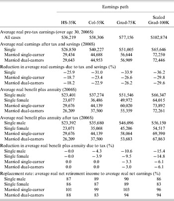
The results from the simulations that account for taxes and savings are presented in Table 4. Prior to retirement, the percentage of gross earnings accounted for by savings and taxes for single individuals ranges from 26% for HS-35K workers to 36% for Scaled Grad-100K workers. Holding total earnings fixed, married individuals have a lower reduction in income from savings and taxes, ranging from 18 to 30%.
Results from simulation accounting for taxes and savingsFootnote 1

Source: Author's calculations.
1 Assumes savings are invested in inflation-indexed bond earning 2.4% real; inflation rates taken from history and Social Security Administration's Intermediate Projection. At retirement, real annuity purchased, with pricing for annuity taken from Vanguard's annuity website on October 31, 2006.
Differences in the percentage of earnings accounted for by savings and taxes are due to several factors. Higher earners and single individuals are assumed to begin saving earlier and (in some cases) contribute a higher percentage of earnings to their 401(k) than do lower earners and married couples. Higher earners pay more income taxes because the taxes are progressive. Married couples pay lower taxes than single individuals for a given level of total earnings because of an additional personal exemption, a higher standard deduction, and different tax rate schedule. Dual-earner couples pay slightly less income taxes in Virginia than single-earner couples because of a spousal earnings credit. Payroll taxes do not contribute measurably to any differences, as the payroll tax as a percentage of earnings differs little among all workers.Footnote 26
Reductions of gross income in retirement are much lower. For single individuals with HS-35K earnings, taxes in retirement are negligible, while for those that have Scaled Grad-100K earnings, the reduction in income is around 15%. For married couples, taxes are negligible for those with HS-35K and Col-55K earnings, and only reduce income by 7% for those with Scaled Grad-100K earnings. Reductions in gross income decline during retirement because there are no payroll taxes or savings during retirement. In addition, income taxes are lower because gross income is lower; Social Security income is at least partially excludable from taxable income; and because of increased deductions and credits.
In the lowermost panel of Table 4 are recorded the new measures of replacement that account for savings and taxes. Replacement rates of net income are much higher than replacement rates of gross income. For single individuals, replacement rates range from 83 to 92%. For married couples, replacement rates range from 83 to 102% of net income. On average, accounting for savings and taxes typically causes the measured replacement rate to increase by 20 percentage points or more.
4.2 Adjusting for owner-occupied housing
Of households with a household head aged 55–64, 79% own a home; and for these home-owning households the net-equity in their house (i.e., the value of the home less mortgage debt) represents, on average, 40% of household net worth.Footnote 27 Of households with a household head aged 65–74, 81% own a home and 49% own a home unencumbered by mortgage debt.
The primary benefit of owner-occupied housing is that it supplies rental services in excess of expenses. That is, if a household does not own a house, they would be required to pay rent to live in a house. At a minimum, a household that owns a dwelling will need less income during retirement than they would if they did not own a home. In addition, owning a home is a hedge against housing services inflation. It is possible that accounting for the option to liquidate some or all of housing wealth would result in calculating even higher well-being during retirement for the simulations in this study, but liquidating home equity is not a component of the replacement rate measure.
To construct a replacement measure that accounts for owner-occupied housing, it is assumed that, if a retiree has paid off his or her mortgage, he/she need not replace the earnings used for paying the principal and interest on the mortgage prior to retirement. The monthly payment for a self-amortizing mortgage consists of two components: a payment to principal and a payment of interest expense. A payment to principal is savings and, like a 401(k) contribution, the savings need not be replaced during retirement. Payment of interest expense, assuming the mortgage is paid off, will not be necessary during retirement. Other expenses of home ownership – property taxes, insurance, and maintenance – are incurred both before and after retirement, and thus are not deducted from pre-retirement earnings.Footnote 28 To measure the adequacy of savings for those households that own a home and have no mortgage debt, average retirement income net of taxes is compared to average pre-retirement earnings net of savings, taxes, and mortgage payments.
To calculate mortgage payments, it is assumed that all individuals and couples: (1) purchase a home at age 35; (2) finance 100% of the purchase price using a 30-year fixed-rate mortgage charging a 7.0% rate of interest; and (3) pay off the mortgage at age 65. The purchase price of the home is assumed to vary by earnings path and is set (approximately) equal to the observed median purchase price of a house in the second quarter of 2006 in specific geographic regions and reported by the National Association of Realtors (2006). In 2006 dollars, the purchase prices are assumed to be $300,000 for the Scaled Grad-100K earnings path (equal to the median purchase price of a home in the northeast region); $230,000 for the Grad-75K earnings path (equal to the median purchase price of a home in all of US); $190 for the Col-55K earnings path (equal to the median purchase price of a home in the southern region); and $100,000 for the HS-35K earnings path (equal to the median purchase price of a home in Buffalo, NY).
Although property taxes are not deducted from the measure of pre-tax income, property taxes are calculated in the process of recalculating income taxes. The real price of the house is assumed to stay constant, with the nominal price increasing at the rate of inflation. Property taxes are assumed to be 1.5 cents per dollar of its value.Footnote 29 As before, simulated taxpayers are assumed to choose the itemization status that minimizes tax burden. However, for Federal income tax purposes, itemized deductions are calculated as state income taxes plus property taxes paid on the house plus mortgage interest expense. For state income tax purposes, itemized deductions are calculated as property taxes plus mortgage interest expense.
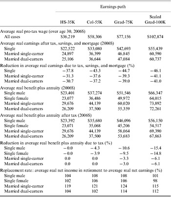
The results of these simulations are presented in Table 5. The effect of accounting for owner-occupied housing is that pre-retirement net income is reduced substantially. Mortgage payments, net of tax benefits, represent 10–15% of average pre-retirement earnings. All told, savings, taxes, and mortgage payments reduce pre-retirement gross earnings, on average, from 30 to 46%. The purchase of a house does not affect income in retirement, thus taxes continue to take anywhere from 0 to 15% from gross retirement income.Footnote 30 The result is that measured replacement rates increase substantially. Replacement rates for single individuals range from 98% for single females with Scaled-Grad 100K earnings to 109% for single males with Col-55K earnings. For married couples, replacement rates range from 102% for split earner couples with Col-55K earnings to 124% for single-earner couples with Grad-75K earnings.
Results from simulation accounting for taxes, savings, and owner-occupied housingFootnote 1

Source: Author's calculations.
1 Assumes savings are invested in inflation-indexed bond earning 2.4% real; inflation rates taken from history and Social Security Administration's Intermediate Projection. At retirement, real annuity purchased, with pricing for annuity taken from Vanguard's annuity website on October 31, 2006.
4.3 Summary of replacement rate measures
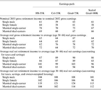
Table 6 summarizes different replacement rate measures. The top panel shows replacement rates that are often reported in retirement studies: nominal income in the first year of retirement relative to nominal income in the year prior to retirement. Moving to a measure that compares retirement income to average earnings boosts measured replacement rates from 3 percentage points to 6 percentage points. Accounting for taxes and savings increases replacement rates by 21–25 percentage points for single individuals and by 16–24 percentage points for married couples. Accounting for owner-occupied housing improves replacement rates another 16–22 percentage points. Altogether, a homeowner with a replacement rate of 60% of gross earnings in retirement, as typically measured, could find that they actually have more income in retirement – net of savings, taxes, and mortgage payments – than they had while working.
Summary of replacement rate results (%)Footnote 1

Source: Author's calculations.
1 Assumes savings are invested in inflation-indexed bond earning 2.4% real; inflation rates taken from history and Social Security Administration's Intermediate Projection. At retirement, real annuity purchased, with pricing for annuity taken from Vanguard's annuity website on October 31, 2006.
4.4 The adequacy threshold
The replacement rate measure developed above corresponds more closely than typical replacement rate measures to a consumption replacement rate. Given the new measure, what then is the threshold for retirement adequacy? A starting point would be to assume that a retiree would want to replace 100% of his average real net earnings, after accounting for savings, taxes, and (if he owns his house) mortgage payments.Footnote 31
However, it could be argued that replacement rates below 100% are adequate. First, there are certain expenses – such as commuting expenses, purchases of lunch and coffee, and buying work clothes – that may be eliminated or reduced during retirement.Footnote 32 Second, households often purchase other long-lived products besides housing (i.e., consumer durables) that continue to provide services well into retirement. Perhaps most importantly, if workers raised children prior to retirement, household expenses presumably would be lower if these individuals or couples are no longer supporting minor children during retirement.Footnote 33
It could also be argued that income needs will increase during retirement, making the threshold of adequacy greater than 100%. The replacement rates presented in this paper are in real terms. However, if retirees consume a different bundle of goods than the average consumer, it is not clear that accounting for inflation is a sufficient adjustment to pre-retirement consumption when measuring adequacy in retirement. For example, health care costs may increase at a faster rate than general inflation and, perhaps more importantly, the amount of health care consumed is likely to increase during retirement. Indeed, increased health care expenditures is the primary argument in favor of an adequacy measure greater than 100%.
Although this paper does not systematically account for health care expenses during retirement, a few points are worth noting. Some retirees, especially at the lower end of the income distribution, may find that the combination of Medicare and Medicaid, as least as currently structured, compares favorably to the health insurance coverage that they had prior to retirement. For those with income or assets that disqualify them for Medicaid coverage, a shortcoming of Medicare coverage is that it will cover only acute medical services; long-term care in an assisted living facility or nursing home is typically not covered. However, as noted above the current calculations assume that the home is used only for providing residential services. If, in fact, home equity were to be tapped during retirement, homeowners would have more resources than suggested by the calculated replacement rates. And, if increased health care needs coincide with a reduced need for residential services – for example, moving from owner-occupied housing into an assisted living facility – selling the residence or renting it out may be an option to generate needed financial assets.
Without modeling these factors explicitly, it is difficult to determine what the adequacy threshold would be using the revised replacement rate measure. For the lower end of the income distribution, it is likely that the adequacy threshold is below 100%. However, depending on the evolution of health care and public policy, there is a risk that future increases in retiree health care expenditures could push the adequacy threshold to 100 or above.
5 Cuts in Social Security benefits
The above discussion regarding health care illustrates the connection between public policy and private action: How much saving is needed for retirement depends in part on future public policy with regard to health care. More directly, future changes to the Social Security system will affect how much private savings is needed for retirement. As widely reported, projected Social Security benefit payments under the current formula are larger than the amount of revenue that is projected to be collected from payroll taxes at current payroll tax rates. To make Social Security sustainable in the long run, either payroll taxes must be increased or benefits must be cut (or some combination of the two). Using assumptions consistent with the SSA's intermediate assumptions, the Congressional Budget Office (2006) projects that the government will no longer be able to finance current law benefits by 2047. They project that revenues in 2049 will be able to finance 79% of current law benefits and by 2100 will only be able to finance 69% of current law benefits. However, benefits cuts that begin earlier and that are phased in can restore balance with less-drastic cuts.Footnote 34
This section examines replacement rates under two scenarios: (1) benefits are cut across-the-board by 28%; and (2) benefits are cut by the use of the so-called ‘progressive indexing’ starting in 2012. Note that these two alternatives are not strictly speaking ‘stable’ reforms. Cutting the benefits by 28% in 2033 would cut benefits more than that would be needed to bring the system into balance. Estimates are that current law benefits could be paid until 1946; a cut in benefits of 28% would not likely be needed until much later in the century. Similarly, progressive indexing from 2012 to 2033 would not bring the system into balance; progressive indexing would likely have to continue beyond 2033 or be coupled with either other benefit cuts or a tax increase. However, these two policy options could be part of a stable reform and they give some indication of the range of Social Security benefits cuts that are contemplated.
The calculation of a 28% across-the-board benefits cut is straightforward. Progressive indexing requires some explanation. When calculating benefit payments, a worker's earnings history (before age 60) is indexed by growth in average wages, not growth in average prices (i.e., inflation). Because nominal wage growth has typically exceeded inflation, the formula, in some sense, gives a worker ‘credit’ for earnings in excess of his real earnings. It has been suggested that the formula be changed to index earnings by inflation rather than wage growth to reduce future benefit payments. Progressive indexing is an alternative to full inflation indexing of the benefit formula. In principle, progressive indexing provides wage indexing for workers below some level of average earnings, provides inflation indexing for workers above a higher level of earnings, and provides a combination of inflation and wage indexing for those in between. In practice, applying progressive indexing to the benefit formula is more complicated. This paper simulates the progressive-indexing proposal described in Purcell (Reference Purcell2005) .Footnote 35
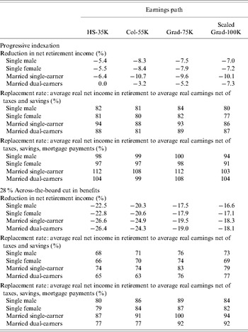
Table 7 presents the results from the simulations that incorporate cuts in Social Security benefits. The top panels examine progressive indexing of benefits. For single individuals, cuts in net retirement income range from 5% for single males with HS-35K earnings to 9% for single females with Scaled Grad-100K earnings. For married couples, cuts in net income range from 3% for married dual earners with Col-55K earnings to 11% for married single earners with Scaled Grad-100K earnings. The benefits cuts represent a larger percentage cut in income for higher earners, with higher earners having larger reductions in income controlling for gender and marital status. Controlling for total income, single individuals and single-earner married couples have larger reductions than dual-earner married couples. Because the earnings of each spouse in a dual-earner married couple with HS-35K earnings is below the hold-harmless level, they do not have a reduction in Social Security benefits.
Results from baseline case simulation1 with cut in Social Security Benefits (%)

Source: Author's calculations.
1 Assumes savings are invested in inflation-indexed bond earning 2.4% real; inflation rates taken from history and Social Security Administration's Intermediate projection. At retirement, real annuity purchased, with pricing for annuity taken from Vanguard's annuity website on October 31, 2001.
Turning to replacement rates, calculated replacement rates with progressive indexing, not accounting for owner-occupied housing, range from about 75 to 85% for single individuals and from about 85–95% for married couples. Accounting for owner-occupied housing, replacement rates range from about 90 to 100% for single individuals and from about 100 to 110% for married couples.
In 2033, a 28% across-the-board cut would represent a much more substantial cut in benefits and net income than would progressive indexing. Despite the fact that all benefits are cut proportionately, these cuts represent a more substantial cut to net retirement income for lower earners and for married couples, because Social Security benefits represent a larger proportion of their retirement income. For example, a 28% cut in Social Security benefits represents nearly a 27% cut in net retirement income for a single-earner married couple with HS-35K earnings, but only a 17% cut in net retirement income for a single individual with Scaled Grad-100K earnings. Thus, unlike progressive indexing, an across-the-board cut in benefits leads to proportionally larger cuts in net income and to generally lower replacement rates for lower-earning individuals and couples. Not accounting for owner-occupied housing, replacement rates range from about 65 to 80%. Accounting for owner-occupied housing, replacement rates generally range from 75 to 90%.
Perhaps not surprisingly, cuts in Social Security benefits would need to be offset by higher personal savings. The modest savings rates assumed in the paper may still be adequate under progressive indexing, particularly for those aged 40 in 2006, and for those who own a own home. Larger across-the-board cuts would likely necessitate much higher levels of personal savings.
6 Sensitivity analysis
The above simulations require assumptions about when an individual retires, when an individual starts savings, and the rate of return earned on savings. This section investigates how sensitive the simulation results are to these assumptions.
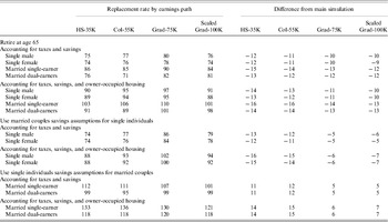
The top panel of Table 8 shows the result of simulations where it is assumed that individuals retire at age 65, two years prior to their normal retirement age. This decision reduces both Social Security benefits and income derived from 401(k) account accumulations. Social Security benefits are reduced by 14–16%, depending upon earnings. The bulk of this cut is caused directly by a  % reduction in calculated Social Security benefits – a 5/9th of one% cut for every month of entitlement before full retirement age. The remainder is due to the fact that the benefit formula is based on an individual's highest indexed earnings of 35 years; retiring early replaces two relatively high earning years with 2 relatively low earning years earlier in the worker's career. Income derived from 401(k) accumulations is reduced both because there are 2 fewer years to accumulate retirement assets and because the cost of an annuity is higher for a 65-year-old than it is for a 67-year-old. In total, income from 401(k) contributions is reduced by 12–18% depending on the age at which individuals begin savings. Because Social Security benefits provide the bulk of retirement income, the drop in retirement income due to early retirement is attributable primarily to the reduction in benefits, despite the fact that decision to retire early causes similar percentage cuts in both Social Security benefits and investment income. However, the relative importance of Social Security benefits varies by earnings and marital status. For example, the reduction in Social Security benefits accounts for nearly 95% of the reduction in gross retirement income for married couples with HS-35K earnings, but only about 55% of the reduction in gross retirement income for single individuals with Scaled Grad-100K earnings.
Sensitivity of replacement rates to age of retirement and savings assumptionsFootnote 1 (%)

1 Assumes savings are invested in inflation-indexed bond earning 2.4% real; inflation rates taken from history and Social Security Administration's Intermediate Projection. At retirement, real annuity purchased, with pricing for annuity taken from Vanguard's annuity website on October 31, 2006.
Overall – combining the reductions in gross retirement income, taxes, and pre-retirement income – retiring at age 65 reduces replacement rates by 9–15 percentage points. For renters, early retirement drops calculated replacement rates to 90% or less for all, with the replacement rate for single individuals being about 75–80%. For homeowners, early retirement replacement rates range from 88 to 110%. The results suggest that the savings assumptions used in the simulations may provide adequate resources for homeowners who wish to retire before the Social Security full retirement age, but that renters may need to save a higher percentage of earnings or begin saving earlier.
Controlling for total household earnings, single individuals are assumed to start saving earlier, and in some cases are assumed to save a higher percentage of their income, relative to married couples. This assumption is not based on marital status, per se, but based on the fact that a two-person household is less well-off than a one-person household with the same income. The lower panels of Table 8 show how sensitive the simulation results are to the savings assumptions. Specifically, the panels show how the results would change if, controlling for total household earnings, single individuals were assigned the savings behavior assumed for married couples and, conversely, married couples were assigned the savings behavior assumed for single individuals. The biggest differences in assumptions are for the lower earners. Single individuals with HS-35K earnings are assumed to save 6% of earnings beginning at age 42, whereas married couples with HS-35K earnings are assumed to save 4% of earnings beginning at age 52. Single individuals with Col-55K earnings are assumed to save 9% of earnings beginning at age 42, compared to 6% of earnings at age 47 for married couples. Higher earning singles are assumed to save the same percentage of earnings as married couples, but are assumed to begin saving at 32, compared to age 37 for married couples with the same total household earnings. Switching the savings assumptions reduces single individuals' replacement rates by 11–16 percentage points – depending upon the individual's gender and the replacement rate measure used – for workers with HS-35K or Col-55K earnings, and by 5–7 percentage points for higher earners. Married couples get nearly symmetric percentage point increases in replacement rates.
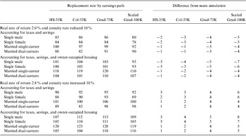
The simulation results are also sensitive to rate of return assumptions. Changes in real interest rates can effect the amount of assets accumulated at retirement as well as the price of the annuity purchased at retirement. To get some idea of the sensitivity of the results, Table 9 reports the results of two sets of simulations that assume different rates of returns and different annuity prices: the first assumes a real rate of return of 2.0%, 40 basis points lower than the baseline assumption, and an annuity that pays 10% less than the baseline simulation for every dollar invested; the second assumes a rate of return of 2.8% and an annuity that pays 10% more than the baseline simulation for every dollar invested.Footnote 36 The replacement rates for single individuals and higher earning individuals are more sensitive to the rate of return assumptions, because 401(k) accumulations finance a higher percentage of retirement income. For example, replacement rates of married couples with HS-35K earnings only increase or decrease 1 percentage point from the baseline assumptions. In contrast, replacement rates of single individuals with Scaled Grad-100K earnings increase or decrease between 5 and 8 percentage points (depending upon gender and the replacement rate measure) relative to the baseline assumptions.
Sensitivity of replacement rates to rate of return and annuity pricing assumptionsFootnote 1 (%)

1 Assumes savings are invested in inflation-indexed bond earning; inflation rates taken from history and Social Security Administration's Intermediate Projection. At retirement, real annuity purchased, with pricing for annuity taken from Vanguard's annuity website on October 31, 2006.
7 Conclusions
To assess retirement preparedness, this paper constructs a replacement rate measure that attempts to measure replacement of pre-retirement consumption – rather than income, earnings, or expenditures – during retirement. This measure accounts for saving, taxes, and (for homeowners) mortgage payments. The simulations in this study show that savings and investment behavior, which would be judged inadequate by standard analysis, in fact results in high real consumption in retirement relative to pre-retirement consumption. For example, the assumed savings and investment behavior of single individuals in the simulations results in traditional replacement rate measures – that is, retirement income to final pay – of approximately 60%, well below the adequacy threshold of 75–80%. However, these ratios correspond to consumption replacement rates of approximately 90% for renters and over 100% for homeowners who have paid off their mortgage.
This paper shows that moderate savings rates – for example, savings of 6% of earnings beginning at age 42 for an individual earning $35,000 a year – can lead to adequate retirement savings. These results do not rely on overly optimistic assumptions about investment returns or require investment in risky assets: savings are investing in TIPS yielding 2.4% above inflation. These results do not ignore the risk of individuals outliving their assets: at retirement individuals invest their retirement assets in an inflation-indexed immediate life annuity.Footnote 37 In addition, the pricing for the annuity reflects actual market prices; it is not a price that is calculated assuming the existence of an actuarially fair annuity.
The results in this paper are consistent with those presented by Sabelhaus (Reference Sabelhaus1997), who also concludes that relatively moderate savings can fund adequate consumption during retirement. By using a replacement rate measure more consistent with consumption smoothening, the results of this paper may also provide an insight into the fact that why studies that use a lifecycle model, such as Engen, Gale and Uccello (Reference Engen, Gale and Cori2004) and Scholz, Seshadri, and Khitatrakun (Reference Scholz, Seshadri and Khitatrakun2006), tend to conclude that most Americans are adequately prepared for retirement, whereas studies that use typical replacement rate methods typically do not. In addition, unlike Munnell, Webb, and Delorme (Reference Munnell, Webb and Delorme2006), who found that accounting for owner-occupied housing has little effect on their measure of retirement preparedness, this analysis illustrates that properly accounting for owner-occupied housing dramatically affects replacement rate measures. Under realistic assumptions, a homeowner's mortgage payments, net of tax benefits, represent 10–15% of average pre-retirement earnings. If the mortgage is paid off before retirement, replacement rates are increased substantially.